Stellar streams around the Magellanic Clouds in 4D

Abstract

We carried out a spectroscopic follow-up program of the four new stellar stream candidates detected by Belokurov & Koposov (2016) in the outskirts of the Large Magellanic Cloud (LMC) using FORS2 (VLT). The medium-resolution spectra were used to measure the line-of-sight velocities, estimate stellar metallicities and to classify stars into Blue Horizontal Branch (BHB) and Blue Straggler (BS) stars. Using the 4-D phase-space information, we attribute approximately one half of our sample to the Magellanic Clouds, while the rest is part of the Galactic foreground. Only two of the four stream candidates are confirmed kinematically. While it is impossible to estimate the exact levels of MW contamination, the phase-space distribution of the entire sample of our Magellanic stars matches the expected velocity gradient for the LMC halo and extends as far as 33 deg (angular separation) or 29 kpc from the LMC center. Our detections reinforce the idea that the halo of the LMC seems to be larger than previously expected, and its debris can be spread in the sky out to very large separations from the LMC center. Finally, we provide some kinematic evidence that many of the stars analysed here have likely come from the Small Magellanic Cloud.

1 Introduction

The Large and Small Magellanic Clouds (LMC and SMC, respectively) are a pair of nearby, likely massive dwarf satellite galaxies, probably orbiting the Milky Way (MW). Located at Galactocentric distances of $\approx$50 and $\approx$60 kpc, respectively, at the moment they are well within the halo of the MW. In the hierarchically assembled Universe, the LMC should have accreted smaller objects whose tidal debris would eventually mix and dissolve in the satellite’s gravitational potential, forming its stellar halo. Therefore, the existence of the LMC stellar halo and its extent and lumpiness could be used to understand some of the details of the structure formation on scales below L${}_{\ast}\sim 2\times 10^{10}L_{\odot}$ (characteristic luminosity of MW and Andromeda-like galaxies).

The scenario in which the LMC had been accreting smaller systems to form its own stellar halo appears to be reinforced by the discovery of a group of ultra-faint objects in the vicinity of the Magellanic Clouds (MCs; Koposov et al., 2015; Bechtol et al., 2015; Drlica-Wagner et al., 2015; Kim & Jerjen, 2015; Drlica-Wagner et al., 2016; Torrealba et al., 2018). Using dynamical models of the LMC in-fall, Jethwa et al. (2016) found that at least one-third of these new objects could be associated with the LMC, with the Cloud’s total dwarf population reaching as many as $\sim$70 in the past. Note that most recently, based on the newly proper motion measurements from Gaia DR2 (Gaia Collaboration et al., 2018; Fritz et al., 2018a), the association to LMC of these dwarfs have been confirmed or disapproved, depending on the sample of member stars considered (see, e.g., Simon, 2018; Kallivayalil et al., 2018; Fritz et al., 2018b; Pace & Li, 2018). Moreover, the complex morphology of HI gas surrounding the MCs (see the review of D’Onghia & Fox, 2016, and references therein), is a living proof of the intricate dynamical interaction history of the LMC and SMC – both between each other and with the MW – of which little has been understood to date. Only recently, based on high precision proper motions derived using the Hubble Space Telescope, the fast tangential motion of the LMC (Kallivayalil et al., 2006; Kallivayalil et al., 2013) has been uncovered, implying a large orbital velocity which in turn favours a recent accretion onto the MW ($<$4 Gyr). This scenario has strong implications for the mass of the Galaxy (Busha et al., 2011) and the genesis of the gaseous Magellanic Stream (MS; e.g., Besla et al., 2010). It has been suggested that close encounters between the LMC and SMC may be responsible for both the gas and stellar structure identified around these galaxies (e.g. Besla et al., 2012; Diaz & Bekki, 2012). Moreover, according to the state-of-the-art simulations of the interaction between the LMC, the SMC and the MW, large sprays of the SMC debris ought to be discovered throughout many sightlines around the LMC (see Besla et al., 2012; Besla et al., 2013; Diaz & Bekki, 2011, 2012; Hammer et al., 2015).

Early attempts to map out the stellar halo of the LMC were based on star count maps (e.g., Irwin, 1991; Kinman et al., 1991) which later were found to be compatible with extended disk models (Alves, 2004), and the kinematics of specific and rare tracers such as RR Lyrae stars (Minniti et al., 2003) and planetary nebulae (Feast, 1968) supporting the existence of an extended spheroidal component. Nonetheless, the LMC stellar disk has been found to stretch as far as $\sim$10 scale-lengths ($\sim$15 deg from the LMC centre, e.g., Saha et al., 2010; Balbinot et al., 2015). Therefore, to study and detect the LMC’s stellar halo, the outskirts of the galaxy need to be explored, where the LMC’s disk is not as overwhelming. For instance, Muñoz et al. (2006) and Majewski et al. (2009) presented the first pieces of evidence for an extended halo-like structure for the LMC traced with spectroscopically confirmed giants in the direction of the Carina dwarf spheroidal galaxy.

With the most recent releases of the wide-field photometry from the Dark Energy Survey (DES, Diehl et al., 2014) and the Gaia mission (Gaia Collaboration et al., 2016), the low-surface brightness structure of the Clouds has started to come into a sharp focus (Belokurov & Koposov, 2016; Mackey et al., 2016; Belokurov et al., 2017; Deason et al., 2017; Pieres et al., 2017; Mackey et al., 2018). These studies provided plenty of tantalizing evidence for the past and ongoing encounters between the Clouds as well as their disruption by the MW. However, what all of these studies have lacked so far is the kinematic dimension. Without the velocity information, it is fatuous to believe that the details of the Clouds’ interaction can be deciphered. In this paper, we describe a spectroscopic effort to provide the missing line-of-sight velocity information for a large sample of stars scattered throughout the Magellanic System. Our targets are selected from the sample of Blue Horizontal Branch (BHB) star candidates from Belokurov & Koposov (2016) and cover a wide range of angular distances from the LMC, i.e. between 13.0 and 48.4 deg. These stars are between 13.0 and 42.0 degrees away from the SMC.

This paper is organised as follows. Section 2 gives the details of the follow-up spectroscopic observations, including the spectral fitting, the separation between Blue Stragglers and the BHBs as well as the metallicity estimation based on the Ca II K line. In Section 3, we discuss the possibility of the Magellanic origin for some of the stars in our sample and compare their distribution in the phase-space to the predictions of the numerical simulations of the Magellanic in-fall. The summary of our study can be found in Section 4.

2 Observations

BHB candidates in the four different substructures (S1-S4) identified by Belokurov & Koposov (2016) were selected for follow-up spectroscopy. Medium-resolution ($R\simeq$ 1 400) spectra were collected at Paranal Observatory, using the FORS2 spectrograph mounted on the VLT UT1 8m telescope. The data were collected during four nights of Visitor Mode observations (Program ID 098.B-0454A) carried out between November 1-5 2016. The exposure times varied from 240s up to 780s, depending on the target magnitude and airmass. The seeing conditions were generally good, with a mean seeing of 0.9$\arcsec$ and with a handful of exposures with somewhat inferior seeing ($\sim$1.5$\arcsec$). The instrument was used with the E2V detector, binning of 2$\times$2, SR collimator and a 1.0$\arcsec$ slit (long-slit mode). The grism used was 1200B+97, with a dispersion of 0.36 $\AA$ per pixel. This configuration provides a wavelength range of 3600 - 5110 Å.

The spectra of 104 targets were obtained. Of these, 25 came from contaminating classes of objects, such as quasi-stellar objects (QSOs), white dwarfs or hot subdwarfs (without any Balmer line). To reduce the contamination, from the second night onwards only stars with colours $(g-i)<0.0$ were considered. This additional colour cut allows us to discard most of the QSOs (Deason et al., 2012). As a result, 79 of the 104 targets observed are likely A-type stars based on the presence of strong Balmer lines.

The data reduction was performed using the ESOREX pipeline provided by ESO. Bias-subtraction, flat fielding correction, spectral extraction, sky correction and wavelength calibration were performed through different recipes of the pipeline. Cosmic ray hits were removed through the optimal extraction as implemented in the pipeline. No further removal was required given that our exposure times are relatively short, under 15 min. The spectra were not flux calibrated. Extracted spectra were normalized using a fifth order polynomial.

2.1 Radial velocities

To fit the Balmer lines, a Sérsic profile (Sérsic, 1968) was adopted:

$$y=a\exp{\left[-\left(\frac{\left|x-x_{0}\right|}{b}\right)^{c}\right]}\text{,}$$ (1)

where the $a$, $b$ and $c$ parameters correspond to the line depth at the line centre, a measure of the line width, and a proxy for the line shape, respectively (see also Xue et al., 2008). The $x_{0}$ coefficient corresponds to the wavelength of the line centre and it is related to the radial velocity, $v_{r}$, by $x_{0}=\lambda_{0}(1+v_{r}/c)$. To perform the spectral fit, we only consider the Balmer lines from $H_{\beta}$ to $H_{\eta}$ (i.e., from $\lambda>3800\,{\AA}$) because a reliable continuum normalization is more difficult for lines at bluer wavelengths. Moreover, we consider that the six Balmer line shapes, for a given star, have the same $b$, and $c$ parameters but different depths. Therefore, the parameters to be estimated were $(a_{1},...,a_{6},b,c,v_{r})$ plus the six parameters from the normalization of the continuum. This model was convolved with a Gaussian profile with $\sigma_{\lambda}$ corresponding to the mean spectral standard deviation of the instrument profile at each pixel.

Figure 1 shows two examples of the continuum-normalized spectra together with the model of the Balmer lines (top panels) and the difference between the data and the fit (bottom panels). In both examples, the normalization of the spectrum tends to be less accurate at the bluest region ($\lambda<4000\,{\AA}$), where most of the Balmer lines are located, leaving less wavelength space for the continuum estimation. For that region, the normalized continuum is located slightly above unity. In contrast, a much better normalization is obtained between H$\beta$, H$\gamma$ and H$\delta$. As judged by the residuals exhibited in the bottom panels, a Sérsic profile provides a high fidelity description of the Balmer lines. The most striking outlier is the Ca II K line at $\lambda\sim 3930\,{\AA}$; in the case of S1 32, it stands out rather clearly, but for the star S1 02, this line is barely noticeable. In what follows, we use the strength of the Ca II K line to estimate the stellar metallicity of our targets.

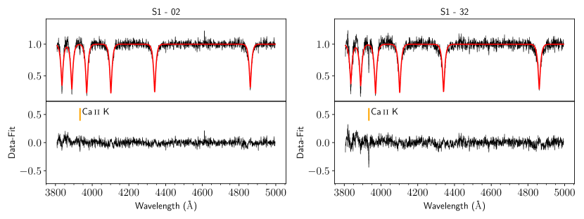
Figure 1: Two examples of reduced spectra for S1 targets. The ID of each target is indicated at the top of each panel. Top panels show the spectra and the fitting of the six Balmer lines plus the continuum normalization. Bottom panels show the residuals from the fit. S1 02 (left) is likely a BHB star while S1 32 (right) is consistent with being a BS, based on the line width and shape of the Balmer lines (see Section 2.2). The spectrum of S1 32 also shows a prominent Ca II line at $\sim 3930\,\AA$.

The 1$\sigma$ error in the fitted radial velocity parameter was adopted as the velocity error. For most of the stars, the radial velocity error is of the order of $\sim$5 km s^-1. Stars in the S4 substructure have the largest errors ($\sim$10 km s^-1) because the collected spectra for these stars have slightly lower S/N than the rest of the sample (S4 is the most distant substructure, located at $\approx$85 kpc). Besides the error associated with the fitting of the Balmer lines, another source of error in the velocity determination is the offset in the centering of the star in the slit. We obtain a rough estimate of this error to be at most $\sim$15 km s^-1 based on the average difference in the derived velocities of stars observed twice and the associated error in the position of H$\beta$ due to a centering offset of about 0.5 pixels (the slit width is 4 pixels), which is the maximum offset allowed between the center of the star and the center of the slit before carrying out the exposures. This is only an upper bound on the actual error and thus it is not included in Table 1. Note that every star would have a slightly different offset in the centering, which is hard to estimate in a star-by-star basis.

2.2 BHB and BS separation

While the most obvious contaminants (such as QSOs, white dwarfs, hot subdwarfs) in our sample were discarded based on the distinct appearance of their spectra, it is not possible (or advisable) to distinguish between the BHBs and the Blue Straggler (BS) stars via visual inspection. Given that Belokurov & Koposov (2016) relied solely on broad-band photometry to define a boundary between the BHBs and the BSs, the cross-contamination of the two classes is not negligible. The main difference between BHB and BS stars is that the former are giant helium-burning stars while the latter are hot dwarf stars on the Main Sequence. Therefore, it is the strength of the surface gravity that differentiates them. Several authors (Rodgers et al., 1981; Kinman et al., 1994; Wilhelm et al., 1999; Clewley et al., 2002; Xue et al., 2008; Vickers et al., 2012) have defined different methods (such as $D_{0.15}$-colour or $D_{0.2}$-$f_{m}$ and the scale-width-shape methods) and the boundaries to separate BHB and BS stars by means of their colours, in addition to Balmer line profiles in medium-resolution spectra. The line profiles alone have been used for this purpose as well.

Most of the previous work, however, only used $H_{\gamma}$ and/or $H_{\delta}$ to study the Balmer line shape. The $b$ and $c$ coefficients of the Sérsic profile are typically used to define the scale-width-shape method to identify the BHB stars (Clewley et al., 2002). Here, the differences in surface gravity are reflected in the $b$ coefficient (scale width), while the effective temperature can be measured through the $c$ (scale shape) parameter.

To take advantage of the good quality of our spectra, below we derive a new boundary for the scale-width-shape method which makes use only of spectroscopic measurements fitting $H_{\beta}$, $H_{\gamma}$ and $H_{\delta}$ simultaneously. To do so, the SDSS DR9 data (Ahn et al., 2012), from which photometry and spectra are available, were explored. We selected A-type stars based on their spectral parameters, $T_{\mathrm{eff}}$ and $\log{(g_{s})}$, and de-redenned colours $(u-g)_{0}$ and $(g-r)_{0}$, as follows:

$$2.8<\log{(g_{s})}<4.6,$$

$$7500<T_{\rm eff}<9300\,[\textrm{K}],$$

$$0.7<(u-g)_{0}<1.4,$$

$$-0.3<(g-r)_{0}<0.0.$$ (2)

Only high S/N spectra (S/N > 20) were considered and borderline cases were excluded (i.e., 3.5 < $\log{(g_{s})}$ < 4.0). Using these cuts, $\sim$2000 A-type stars were selected, for which at least 6 Balmer lines were visible in the wavelength range covered by the SDSS.

Following the same procedure as with our FORS2 data, a polynomial of fifth order plus three Sérsic lines were fitted to the SDSS spectra, this time convolved with a Gaussian profile with $\sigma$ corresponding to the instrument profile (available for each SDSS spectrum), in the wavelength range from $\lambda\approx 4000$ to 5000 Å. Figure 2 shows the effective temperature and the surface gravity (left panel) for this SDSS sample, $T_{\rm eff}$ against the line width parameter $b$ (middle panel), and the two normalized Sérsic parameters $b^{\prime}$ and $c^{\prime}$ (right panel), defined as they both have zero mean and unit variance, with 9.68, 1.70 and 0.89, 0.11 as the mean and standard deviation of $b$ and $c$, respectively. The separation between BHBs and BSs is evident in all the panels, in particular for the stars hotter than 8300 K or $b^{\prime}>-0.5,c^{\prime}>0$. Based on the evident separation between BHBs and BSs in this plane, a separation boundary can be established. To do so, a Support Vector Machine (SVM) was used, as implemented in the scikit-learn module (Pedregosa et al., 2011), using a linear kernel. The derived boundary has the form

$$-0.78\,{c^{\prime}}^{2}+0.6\,{b^{\prime}}^{2}-0.36\,b^{\prime}\,c^{\prime}+2.05\,c^{\prime}-2.61\,b^{\prime}+0.34=0.$$ (3)

From this equation, the boundary function B(c) was defined. Stars with $b^{\prime}$ and $c^{\prime}$ parameter values above this boundary division are most likely BSs, while those below are most likely BHBs. However, those stars that are located close to the boundary can be easily misclassified as the SDSS spectra used to derive the SVM do not include stars with surface gravities between $3.5<\log{(g_{s})}<4.0$, where BHBs and BSs tend to overlap. For the training set, the boundary found allows a separation between BHBs and BSs with a completeness of BHBs of 99% and a contamination of 18% of BSs in the BHB class. These values are in stark contrast to the completeness and purity of photometrically-selected BHB stars: Vickers et al. (2012) reported a 57% completeness and 25% contamination (mostly from MS A-type stars) for SDSS $(u-g)$,$(g-r)$ color-cut selections (in good agreement with previous estimates by Sirko et al., 2004; Bell et al., 2010), while similar completeness and contamination values are found when using SDSS $(g-r)$,$(iz)$ color-cuts (51% and 23%, respectively). A slightly better completeness sample was obtained by Fukushima et al. (2018) when using the z-band photometry from the Hyper Suprime-Cam Subaru Strategic Program, with 67% completeness and 38% contamination.

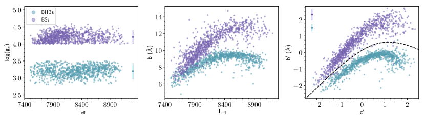
Figure 2: Spectral properties for BHB and BS stars from SDSS DR9. The left panel shows the effective temperature and surface gravity of $\simeq$ 2000 A-type stars, color-coded according to their most likely classification as BHB and BSs based on the surface gravity. The mean uncertainty in the $\log{g}$ estimate, for each sample, is represented by two errorbars located at the top left corner. The middle panel shows the $b$ parameter of the Sérsic profile for the Balmer lines in those spectra as a function of the effective temperature. BHBs tend to have smaller $b$ values, i.e., narrower lines, than BSs. The right panel shows the $b^{\prime}$ and $c^{\prime}$ parameters of the Sérsic profile (see text) and the separation between BHBs and BSs as derived in this work (equation 3, dashed line), while at the top left, the mean error of the coefficients is represented by two errorbars.

For our sample, the classification was carried out based on the Sérsic parameters for the same three Balmer lines available in the SDSS spectra. The results of the fitting are shown in Figure 3. Top row panels show the targets colour-coded by the probability to belong to the BHB class according to the division boundary given by the SVM. The dashed line shows the boundary as defined in Eq. 3. Stars that are at the edge have probabilities between the two classes and are marked with open squares. They are listed as “BHB/BS” in Table 1. In the top left panel, the same parameter space as for SDSS stars is shown. The separation shows that most of the stars can be classified as either a BHB or a BS with high confidence. The top middle panel shows the $c^{\prime}$ parameter as a function of the difference between $b^{\prime}$ and Eq. 3. In this plane, BS stars are clearly confined to large [$b^{\prime}$ - B(c)] values as compared to the BHBs. The top right panel shows [$b^{\prime}$ - B(c)] versus the Galactic Standard of Rest (GSR) velocities (derived from the fitting of the six Balmer lines in the spectra). At the boundary, there is a group of four stars with $V_{\rm GSR}$ greater than 100 km s^-1 that cannot be unequivocally classified as BHB or BSs (marked with open squares). The bottom row of panels in Figure 3 shows the distribution of $b^{\prime}$, $c^{\prime}$ and $V_{\rm GSR}$ for our stars, colour-coded according to the (tentative) substructure they belong to: blue for S1, green for S2, yellow for S3 and red for S4. Stars from S4 tend to have the largest error bars, likely because their spectra have lower S/N (Sect. 2.1). At the boundary, three stars from S1, one from S2, four from S3 and two stars from S4 can be either BHB, BS and, therefore, are not excluded from the remaining analysis but marked in every plot with an open square symbol.

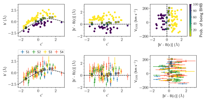
Figure 3: Stellar classification among BHB and BS stars from our FORS2 observations. The top row shows the target stars color-coded by to the probability of being classified as BHBs. At the bottom row, the stars are colour-coded according to the substructure they tentatively belong to: blue for S1, green for S2, yellow for S3 and red for S4. Left panels show the $b^{\prime}$ and $c^{\prime}$ coefficients from the Sérsic profile, and the boundary derived based on SDSS data. In the middle panels, the $c^{\prime}$ coefficient and the difference between the $b^{\prime}$ parameter and the corresponding $b^{\prime}$ from equation 3 is shown. The rightmost panels present [$b^{\prime}$ - B(c)] against $V_{\rm GSR}$. Stars marked with open squares are those which can be either BHB or BS as they are located just at the separation boundary between the two classes.

2.3 Heliocentric distances

Once the stars have been classified as BHB or BSs, the heliocentric distance can be derived accordingly. The distances for the BHB stars were derived using the absolute magnitude equation given in Belokurov & Koposov (2016). The dispersion of this relation is $\simeq$0.1 mag.

Absolute magnitudes for the BS candidates were determined considering the $V$-band relation given in Eq. (14) by Kinman et al. (1994). To transform from the Johnson $V$ magnitude into Sloan $g$, the colour and magnitude relations from Jester et al. (2005) were used. Combining all the relations, we derive the equation for the $g$-band absolute magnitude of BSs as

$$M_{g}=2.2+4.557(g-r)_{0}-0.45{\rm[Fe/H]}.$$ (4)

This relation is slightly different from the one derived by Deason et al. (2011). At a fixed metallicity, and depending on the $(g-r)_{0}$ colour, the difference between the relations can be as high as 0.2 mag. Nonetheless, the dispersion of the relation from Deason et al. (2011) is greater, of $\simeq$0.5 mag. To be conservative, the same intrinsic dispersion is adopted for our relation, despite taking into consideration the metallicity dependence on the absolute magnitude of BSs. The distances for the BS candidates were derived adopting a metallicity of [Fe/H]=$-1.5$. This value is a compromise between the metallicities of the MW stellar halo, the LMC and the SMC.

Figure 4 shows the Galactocentric distances of the BHB and BS stars for the four different sub-structures as a function of the MS longitude, $L_{\rm MS}$ (defined by Nidever et al., 2008). The stars with uncertain classification were included in both panels, with the according distance if they are considered BHB or BSs, respectively, and marked with open squares. All of the BHBs are located at $R>40$ kpc, reaching out to $\simeq$100 kpc, far away from the effective radius of the MW halo. For the BSs, the distances are smaller, and most of them can be considered members of the MW halo. Indeed, the typical break radius of the Galactic halo, beyond which the stellar density falls-off more rapidly, is $\sim$25 – 30 kpc (see e.g., Deason et al., 2011; Xue et al., 2015; Bland-Hawthorn & Gerhard, 2016, and references therein). As a conservative cut, all the BSs at $R<$ 35 kpc hereinafter will be considered to be part of the MW halo, while those with $R\geq 35$ kpc are most likely members of the MCs. There are one BS from S2, three from S3 and eleven from S4 that passed this cut, and are included in the remaining analysis along with all the BHBs.

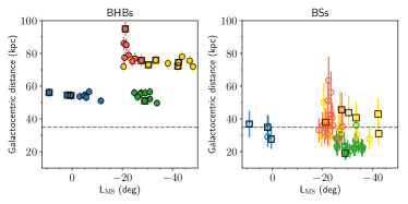
Figure 4: Galactocentric distances for BHB (left) and BS (right) stars as a function of $L_{\rm MS}$. The colours are the same as in Figure 3. Stars marked with open squares correspond to those that can be either BHB or BSs and therefore the corresponding distance in each case is considered. The dashed line marks the break radius at $\sim 35$ kpc. Stars with Galactocentric distances greater than this cut most likely belong to the LMC than to the MW halo.

Table 1 summarizes the properties of all A-type stars with spectra from FORS2. The ID, equatorial coordinates (J2000.0) and the apparent $g$ magnitude from the DES data release 1 (DR1) are listed in columns (1)-(4); column (5) lists their GSR velocities, in km s^-1, while the heliocentric distances, in kpc, are shown in column (6). The distances were derived based on the classification of the stars as BHB or BS and the adopted errors are the result of the propagation of the uncertainty in the relation used: 0.1 mag for BHBs, and 0.5 mag for BSs. For stars with no certain classification, the two possible distances (if being a BHB or a BS) are reported. Column (7) shows the equivalent width (EW) of the Ca II K line. There is no EW measurement for those stars in which the line was too shallow (see Section 2.4). The class (BHB or BS) and the tentative origin, MCs (for all the BHBs and BSs with Galactocentric distances greater than 35 kpc), or MW (BSs with distances lower than 35 kpc) are listed in Columns (8) and (9), respectively. The reported velocities were first converted into heliocentric velocities using the barycentric correction from the rvcorrect task of IRAF and after that transformed to the Galactic Standard of Rest. The reported velocity errors do not consider possible systematic offsets due to imperfectly-centered position of the stars in the slit, which we estimate to be not larger than $\sim$ 15 km s^-1.

2.4 Calcium as a proxy of metallicity

Given the medium resolution of our spectra and the wavelength coverage containing little other features apart from the Balmer lines, we do not attempt to derive the stellar parameters of our target stars. Nonetheless, most of the target spectra show the Ca II K line at $3933\,{\AA}$, particularly the BS stars. The EW of Ca II line can be used as a reliable metal abundance indicator in A-type stars (see e.g., Wilhelm et al., 1999; Clewley et al., 2002; Kinman & Brown, 2011). Therefore, we make use of this line as a proxy for metallicity, as well as an additional statistic to test for the presence of different stellar populations among our targets.

To measure the EW of the Ca II K line, a Gaussian fit to the normalized spectrum was performed. From the width of the line the EW was measured. Figure 5 shows two examples, for S3 05 and S3 17, where the line is shallower (top) and deeper (bottom). The spectra are vertically offset for clarity. The errors on the EW measurements are the propagation of the errors on the fit parameters for the line profile. Overall, the EWs tend to be higher for BSs compared to BHB stars, in agreement with the fact that BHBs are metal-poor stars.

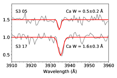
Figure 5: The normalized spectrum of S3 05 and S3 17 in the spectral range around the Ca II K line are shown, vertically offset for clarity. The Gaussian fitting to the Ca II K line is shown in the solid red lines. The EW of the Ca II K line is at the right side of each spectrum.

Figure 6 shows the line-of-sight velocity as a function of the Ca II EW measurements. Only the stars classified as BHBs (filled circles), the distant BSs (open circles) and those without clear classification (open squares) are displayed (i.e., MW stars are not included). The four panels correspond to the four candidate substructures, as indicated on top of each panel. For S1 BHBs, there appears to be a correlation between the velocity and the width of the Ca II line or at least two groups with the EWs greater or lower than 1.0 Å. For S2, all BHBs have similar Ca II EWs and, moreover, all but one very similar V_GSR (with a velocity dispersion of $\sim$ 16 km s^-1). The fact that it is not possible to claim any significant metallicity difference among the S2 BHBs together with their relatively low velocity dispersion supports the hypothesis of Belokurov & Koposov (2016) that S2 is a stand-alone substructure in the LMC halo. S3 and S4 stars (bottom row of panels) are a mix of BHBs and BSs. In general, in BS stars, the EW of the Ca II line is higher, while the BHBs show a narrow range of the EW measurements. This is not the case for one BHB/BS star in S3 with an EW of $\sim$2.0 Å and two BHB/BS from S4 with an EW$>$ 3.0 Å, but these could be just because the stars are actually BSs despite the classification was not certain. There is only one exception: one BHB star in S4 which has EW$>$1.5 Å, greater than any other BHB in that substructure. Overall, we identify a difference in metallicity only in S1 stars, which is reinforced by the two different velocity trends analyzed in Section 3.

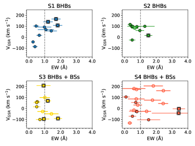
Figure 6: EW of the Ca II K line as a function of the velocity $V_{\rm GSR}$ for the four different substructures. BHB and BS stars are marked as filled and open circles, respectively. The stars can be tagged as “metal-rich” and “metal-poor” at the boundary of EW = 1.0 Å (vertical dashed line).

To quantify the difference in metallicity between the “metal-rich” and the “metal-poor” BHB and BS stars, we derive empirical relations between the Ca EW and [Fe/H] for a bigger sample of A-type stars, following a similar procedure as the one used by Wilhelm et al. (1999). Namely, A-type stars were recovered from SDSS DR9, imposing the same colour cut in $(g-r)_{0}$ as the ones used to select BHB candidates by Belokurov & Koposov (2016), and adding cuts in $(u-g)_{0}$ colour and stellar parameters as follows:

$$0.9<(u-g)_{0}<1.4\text{,}$$

$$-0.30<(g-r)_{0}<-0.05\text{,}$$

$$2.8<\log{(g_{s})}<4.6\text{,}$$

$$7500\text{ K}<T_{\rm eff}<9300\text{ K,}$$

$$S/N>30\text{.}$$ (5)

With this query, $\approx$1000 spectra were recovered. To be consistent with the EW determination of the Ca II line used above for our target stars, the same approach was used for the SDSS A-type stars, i.e. fitting a Gaussian to the Ca line profile in the normalized spectrum. Using the spectroscopic stellar parameters from the SDSS SEGUE Stellar Parameter Pipeline (see Lee et al. 2008 for details), we investigated the correlation between the EW of Ca and effective temperature, surface gravity and [Fe/H]. Figure 7 shows the EW of Ca as a function of the effective temperature for all the sample (left panel), stars with $2.8<\log{(g_{s})}<3.5$ (mainly BHB stars, middle panel), and stars with higher surface gravities, $4.0<\log{(g_{s})}<4.6$ (mainly BSs, right panel), color-coded according to the [Fe/H] values. From the figure, it is evident that the EW of Ca is a strong function of effective temperature and [Fe/H], as previously claimed by Wilhelm et al. (1999) and Clewley et al. (2002). Moreover, the EW of Ca is more sensitive to metallicity for cooler stars, whereas the EW of Ca tends to zero for the hottest (bluest) stars. Given the marked difference between BHBs and BSs, the relations converting EW of Ca into [Fe/H] need to be treated separately.

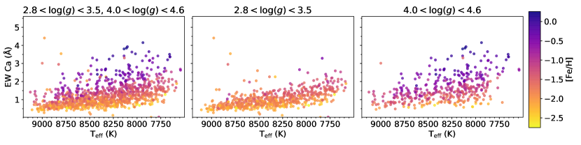
Figure 7: Equivalent widths of the Ca II K line as a function of the effective temperature for A-type stars in SDSS DR9, colour-coded according to the metallicity [Fe/H]. From left to right, the logarithm of the surface gravity ranges are: 2.8 $<\log{(g_{s})}<$3.5 and 4.0$<\log{(g_{s})}<$4.6 (including both BHB and BS star candidates); 2.8$<\log{(g_{s})}<$3.5 (BHB star candidates); 4.0 $<\log{(g_{s})}<$ 4.6 (BS star candidates). For a given temperature, the scatter in the EW of Ca is due to the metallicity difference.

The quadratic relations fitted to the SDSS data are shown in the top panels of Figure 8, separately for the BHBs and the BSs. For both stellar types, for a given value of EW of Ca, there is a range of possible values of [Fe/H], indicative of the dependence of the line shape properties on effective temperature. To correct for this effect, we fit an additional $(g-r)_{0}$ color term to the residuals. The relations to convert from Ca EW and $(g-r)_{0}$ into [Fe/H] for BHB and BS stars are the following

$${\rm[Fe/H]}_{\rm BHB}=-0.2\,\left(\text{EW Ca}\right)^{2}+1.47\,\left(\text{EW Ca}\right)-1.77\,(g-r)-3.26\text{,}$$

$${\rm[Fe/H]}_{\rm BS}=-0.14\,\left(\text{EW Ca}\right)^{2}+1.23\,\left(\text{EW Ca}\right)-2.08\,(g-r)-2.90\text{.}$$

The bottom panels in Figure 8 give the residuals for the SDSS data and the relations derived, showing no correlation with colour and a small dispersion around zero (1$\sigma$ dispersion of 0.25 dex for both BHB and BS stars). Table 3 shows the metallicity estimation for our target stars based on the relations derived from the SDSS data according to their classification as BHB or BS star. In the cases of uncertain classification, metallicities using both BHB and BS relations are presented. The errors were derived from the propagation of the error on the EW of Ca measurement and the errors on the coefficients of the relation used but do not consider the intrinsic dispersion of the relations. For stars as hot as our targets, the SDSS pipeline relies heavily on the Ca II K line to derive metallicities given that only weak iron lines are available. Our approach is based on the same feature, the Ca II K line, which gives us confidence that our metallicity estimates are compatible with the SDSS [Fe/H] estimates.

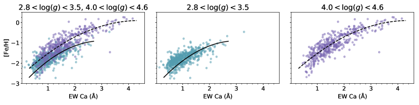
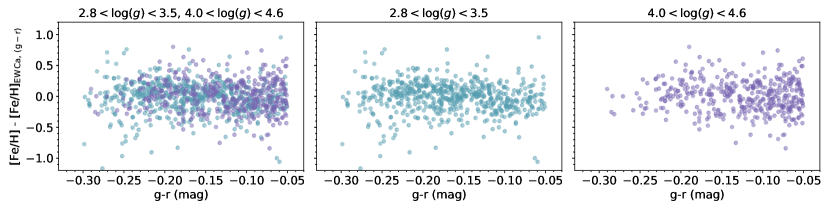
Figure 8: Top panels: Equivalent width of Ca II K line versus metallicity [Fe/H] in the same three surface gravity ranges as in Figure 7. The solid and dashed lines correspond to [Fe/H] as a function of the Ca EW relations derived for BHB and BS stars. Bottom panels show the residuals of the fit, including an additional colour term, as a function of the $(g-r)$ colour, in the same three surface gravity ranges.

Prior to deriving the metallicities from the Ca EWs and $(g-r)$, the interstellar contribution to the EW of the Ca line was also derived (Beers, 1990; Kinman & Brown, 2011). The relations derived are based on the measured EW of Ca and do not take into account the contribution from the interstellar Ca along the line of sight. However, we do not correct for this contribution since the available relations (e.g., Beers, 1990; Kinman & Brown, 2011) are derived based only on Galactic A-type stars. As far as we are aware, there are no corrections for interstellar Ca in stars belonging to the MCs. Using the relations for Galactic stars given by Kinman & Brown (2011), we re-derive the relations converting EWs into metallicities using SDSS stars, and our metallicity estimates for our targets, finding that overall the differences are small (below 0.1 dex). The small contribution of the interstellar material on the measured Ca II line is also evident when the derived [Fe/H] are compared to the extinction E(B-V) values for our targets (derived from the dust maps of Schlafly & Finkbeiner, 2011): there is no correlation between both quantities, indicating that the measured EWs in our targets are not highly affected by the interstellar material along the line of sight. However, other effects could affect our measurement of [Fe/H] using the Ca line such as accretion of interstellar material or atomic diffusion (Brown et al., 2006), in addition to possible star-to-star variations in [$\alpha$/Fe]. Therefore, the presented [Fe/H] values should be considered only as an approximate estimate. For the interested reader, a detailed study of interstellar Ca II absorption in the Milky Way was conducted by Murga et al. (2015).

3 The LMC/SMC connection

The celestial positions of our target stars, in Magellanic coordinates, are shown in Figure 9. Also shown in the figure, underlying the BHB and BS stars, is the density of the BHB candidate stars selected from the DES DR1 photometry using similar colour cuts as described in Belokurov & Koposov (2016): $(g-r,i-z)$ = (–0.40, –0.20), (–0.30, –0.15), (–0.25, –0.13), (–0.20, –0.12), (–0.13, –0.10), (–0.05, –0.09), (0.00, –0.09), (0.00, 0.00), (–0.10, 0.00), (–0.20, –0.02), (–0.30, –0.06), (–0.40, –0.14). From this density distribution alone, the more metal-rich BHBs from S1 (pale blue) can be associated with a disturbed portion of the LMC disk, while the rest of the group extends much further away, not only in Magellanic longitude but also in latitude, further away from the MS, while stars from S2, S3 and S4 are located closer to the MS but further away from the LMC itself.

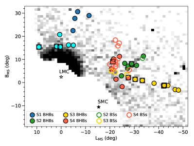
Figure 9: Spatial distribution in Magellanic coordinates (L_MS, B_MS) of BHB stars from the DES survey with our target stars overplotted with filled circles for BHB and open circles for BS stars. S1 stars with high and low relative metallicity are in cyan and blue, while S2, S3 and S4 stars are in green, yellow and red colours, respectively. The position of the LMC and SMC are marked with star symbols and labelled accordingly.

Table 1: A-type stars from the FORS2 observations.

ID	RA (J2000.0)	DEC (J2000.0)	$g$	$V_{\rm GSR}$	$D$	$W$ Ca	Class	Group
	(deg)	(deg)	(mag)	(km s-1)	(kpc)	(Å)
S1 01	69.47791	–41.67166	19.12	–85.7 $\pm$ 6.1	48 $\pm$ 2	0.4 $\pm$ 0.2	BHB	MCs - M1
S1 02	75.92958	–44.00163	19.02	17.9 $\pm$ 4.7	50 $\pm$ 2	0.7 $\pm$ 0.2	BHB	MCs - M1
S1 03	75.24083	–40.96847	19.30	–42.5 $\pm$ 5.2	53 $\pm$ 2	0.3 $\pm$ 0.1	BHB	MCs - M1
S1 16	98.09583	–55.92491	19.39	140.6 $\pm$ 8.5	55 $\pm$ 3/ 35 $\pm$ 8	1.2 $\pm$ 0.3	BHB/BS	MCs - M1
S1 28	85.51833	–56.58208	19.30	107.7 $\pm$ 7.8	53 $\pm$ 2/ 33 $\pm$ 8	1.8 $\pm$ 0.3	BHB/BS	MCs - M1
S1 30	85.39375	–54.35069	19.07	–55.0 $\pm$ 7.0	27 $\pm$ 6	0.5 $\pm$ 0.2	BS	MW
S1 32	82.94583	–56.78797	19.12	165.8 $\pm$ 6.8	53 $\pm$ 2/ 26 $\pm$ 6	1.7 $\pm$ 0.3	BHB/BS	MCs - M1
S1 38	77.15333	–55.72430	19.13	57.4 $\pm$ 5.4	52 $\pm$ 2	1.4 $\pm$ 0.4	BHB	MCs - M1
S1 43	73.76208	–55.52858	19.23	69.3 $\pm$ 6.4	53 $\pm$ 2	1.1 $\pm$ 0.5	BHB	MCs - M1
S1 50	83.41541	–51.45541	19.11	92.7 $\pm$ 5.6	52 $\pm$ 2	1.0 $\pm$ 0.4	BHB	MCs - M1
S1 57	84.92083	–47.85800	19.22	–148.2 $\pm$ 8.3	31 $\pm$ 7	0.8 $\pm$ 0.3	BS	MW
S1 63	75.74666	–49.33027	19.10	101.8 $\pm$ 5.0	52 $\pm$ 2	0.5 $\pm$ 0.2	BHB	MCs - M1
S2 01	30.75012	–57.10719	19.49	99.4 $\pm$ 8.2	57 $\pm$ 3	0.4 $\pm$ 0.3	BHB	MCs - M2
S2 02	32.34349	–55.39111	19.30	–116.7 $\pm$ 7.9	28 $\pm$ 6	1.3 $\pm$ 0.3	BS	MW
S2 04	34.09958	–53.90825	19.28	164.6 $\pm$ 7.3	21 $\pm$ 5	2.2 $\pm$ 0.3	BS	MW
S2 05	35.28941	–53.59127	19.20	29.6 $\pm$ 10.5	23 $\pm$ 5	1.4 $\pm$ 0.2	BS	MW
S2 08	32.28366	–53.11711	19.19	99.6 $\pm$ 5.5	55 $\pm$ 3	1.3 $\pm$ 0.6	BHB	MCs - M2
S2 09	33.14850	–52.25447	19.25	116.5 $\pm$ 5.5	56 $\pm$ 3	0.3 $\pm$ 0.2	BHB	MCs - M2
S2 10	30.53904	–51.97269	19.22	–92.4 $\pm$ 7.0	22 $\pm$ 5	1.1 $\pm$ 0.3	BS	MW
S2 12	31.98020	–50.74277	19.15	96.9 $\pm$ 6.3	56 $\pm$ 3	0.8 $\pm$ 0.2	BHB	MCs - M2
S2 13	31.93720	–50.54833	18.99	11.6 $\pm$ 6.7	18 $\pm$ 4	2.5 $\pm$ 0.3	BS	MW
S2 14	30.02499	–49.50663	19.50	–25.2 $\pm$ 5.2	52 $\pm$ 2	0.5 $\pm$ 0.2	BHB	MCs - M1
S2 15	33.94395	–50.19563	19.34	–22.4 $\pm$ 5.5	23 $\pm$ 5	0.7 $\pm$ 0.2	BS	MW
S2 17	31.46258	–46.86097	19.07	76.7 $\pm$ 8.7	21 $\pm$ 5	0.2 $\pm$ 0.5	BS	MW
S2 18	30.23741	–46.61547	19.19	157.9 $\pm$ 6.3	26 $\pm$ 6	0.9 $\pm$ 0.3	BS	MW
S2 19	31.68004	–46.01044	19.10	24.9 $\pm$ 6.7	21 $\pm$ 5	2.2 $\pm$ 0.3	BS	MW
S2 20	31.35933	–45.65191	19.42	82.8 $\pm$ 6.4	35 $\pm$ 8	0.6 $\pm$ 0.2	BS	MCs - M2
S2 21	32.33658	–44.16247	19.14	–76.8 $\pm$ 6.6	22 $\pm$ 5	0.6 $\pm$ 0.2	BS	MW
S2 25	32.24987	–42.47661	19.30	–101.8 $\pm$ 5.6	21 $\pm$ 5	0.6 $\pm$ 0.2	BS	MW
S2 27	33.65883	–40.94358	19.07	–39.7 $\pm$ 6.1	20 $\pm$ 5	1.7 $\pm$ 0.3	BS	MW
S2 28	30.14699	–55.76855	19.07	–87.7 $\pm$ 6.4	28 $\pm$ 6	0.7 $\pm$ 0.2	BS	MW
S2 29	36.17920	–52.50597	19.19	61.3 $\pm$ 4.4	53 $\pm$ 2	1.0 $\pm$ 0.3	BHB	MCs - M2
S2 30	33.87925	–51.79997	19.17	–9.4 $\pm$ 6.4	30 $\pm$ 7	0.2 $\pm$ 0.2	BS	MW
S2 31	30.08287	–50.65188	19.02	–56.1 $\pm$ 6.3	21 $\pm$ 5	1.1 $\pm$ 0.2	BS	MW
S2 32	32.85958	–50.57858	18.93	16.6 $\pm$ 5.2	51 $\pm$ 2/ 18 $\pm$ 4	1.5 $\pm$ 0.2	BHB/BS	MCs - M2
S2 33	34.90295	–46.74211	19.14	40.4 $\pm$ 6.3	19 $\pm$ 4	2.3 $\pm$ 0.3	BS	MW
S2 34	32.03433	–44.77616	18.92	98.0 $\pm$ 4.8	49 $\pm$ 2	0.5 $\pm$ 0.2	BHB	MCs - M2
S2 35	33.82012	–41.15047	19.00	–101.8 $\pm$ 6.3	19 $\pm$ 4	1.1 $\pm$ 0.2	BS	MW
S3 01	10.40004	–44.47533	19.95	–92.0 $\pm$ 7.3	73 $\pm$ 3/ 44 $\pm$ 10	1.8 $\pm$ 0.3	BHB/BS	MCs - M1
S3 02	9.692750	–42.87016	19.98	14.9 $\pm$ 7.2	79 $\pm$ 4	0.5 $\pm$ 0.2	BHB	MCs - M2
S3 03	10.61537	–44.17408	19.84	68.8 $\pm$ 5.3	76 $\pm$ 3/ 31 $\pm$ 7	1.2 $\pm$ 0.2	BHB/BS	MCs - M2
S3 05	6.025458	–40.76222	19.99	61.6 $\pm$ 6.6	77 $\pm$ 4	0.5 $\pm$ 0.2	BHB	MCs - M2
S3 06	5.101791	–39.58691	19.90	52.5 $\pm$ 6.5	73 $\pm$ 3	0.5 $\pm$ 0.2	BHB	MCs - M2
S3 08	39.95100	–59.46427	19.89	–38.6 $\pm$ 7.7	30 $\pm$ 7	0.8 $\pm$ 0.3	BS	MW
S3 09	39.27050	–58.68730	20.07	–28.4 $\pm$ 8.7	50 $\pm$ 12	0.9 $\pm$ 0.3	BS	MCs - M1
S3 10	36.12066	–57.91583	19.97	–49.6 $\pm$ 11.9	38 $\pm$ 9	1.4 $\pm$ 0.4	BS	MCs - M1
S3 12	35.49362	–57.60886	19.80	72.1 $\pm$ 9.2	29 $\pm$ 7	1.2 $\pm$ 0.3	BS	MW
S3 15	29.44429	–55.67291	19.92	30.1 $\pm$ 16.0	34 $\pm$ 8	…	BS	MW
S3 16	29.18641	–55.00816	20.01	99.0 $\pm$ 8.2	46 $\pm$ 11	1.0 $\pm$ 0.3	BS	MCs - M2
S3 17	29.15583	–54.97430	19.99	43.4 $\pm$ 8.6	32 $\pm$ 7	1.6 $\pm$ 0.3	BS	MW
S3 19	22.72979	–53.51613	19.97	207.4 $\pm$ 8.5	74 $\pm$ 3/ 44 $\pm$ 10	0.9 $\pm$ 0.4	BHB/BS	MCs - M2
S3 22	14.34962	–47.61008	19.83	–101.5 $\pm$ 7.3	75 $\pm$ 3	0.7 $\pm$ 0.2	BHB	MCs - M1
S3 23	14.72145	–46.90730	19.81	120.1 $\pm$ 7.4	28 $\pm$ 6	1.5 $\pm$ 0.4	BS	MW
S3 24	19.52979	–51.26036	19.97	–96.7 $\pm$ 7.1	77 $\pm$ 4/ 41 $\pm$ 9	0.9 $\pm$ 0.3	BHB/BS	MCs - M1
S3 25	19.34391	–50.92566	19.90	88.3 $\pm$ 7.8	30 $\pm$ 7	1.2 $\pm$ 0.3	BS	MW
S4 02	40.13054	–58.00400	20.69	104.2 $\pm$ 8.9	86 $\pm$ 4	0.1 $\pm$ 0.2	BHB	MCs - M2
S4 04	39.12958	–57.69111	20.12	85.8 $\pm$ 7.8	35 $\pm$ 8	0.7 $\pm$ 0.5	BS	MCs - M2
S4 06	43.52183	–56.88783	20.28	204.5 $\pm$ 11.0	35 $\pm$ 8	1.8 $\pm$ 0.6	BS	MCs - M2
S4 12	39.12945	–56.18783	20.19	161.4 $\pm$ 10.3	36 $\pm$ 8	2.5 $\pm$ 0.4	BS	MCs - M2
S4 16	40.25579	–55.29122	20.60	30.5 $\pm$ 6.2	63 $\pm$ 15	0.8 $\pm$ 0.3	BS	MCs - M2

Table 2: continued

A-type stars from the FORS2 observations. ID RA (J2000.0) DEC (J2000.0) $g$ $V_{\rm GSR}$ $D$ $W$ Ca Class Group (deg) (deg) (mag) (km s^-1) (kpc) (Å) S4 17 43.06666 –55.22061 20.32 –3.5 $\pm$ 7.9 95 $\pm$ 4/ 37 $\pm$ 9 3.4 $\pm$ 0.4 BHB/BS MCs - M1 S4 18 41.58354 –54.76944 20.35 180.4 $\pm$ 17.0 51 $\pm$ 12 0.6 $\pm$ 0.7 BS MCs - M2 S4 22 45.46570 –48.95708 20.20 –31.0 $\pm$ 9.0 34 $\pm$ 8 2.1 $\pm$ 0.4 BS MW S4 26 47.22491 –48.60963 20.70 44.3 $\pm$ 8.1 55 $\pm$ 13 2.4 $\pm$ 0.3 BS MCs - M2 S4 28 47.69408 –47.35980 20.62 75.0 $\pm$ 11.9 39 $\pm$ 9 1.8 $\pm$ 0.5 BS MCs - M2 S4 29 50.65604 –47.11874 20.54 172.6 $\pm$ 8.8 40 $\pm$ 9 0.8 $\pm$ 0.3 BS MCs - M2 S4 31 31.35824 –59.81124 20.15 53.9 $\pm$ 6.9 80 $\pm$ 4 0.7 $\pm$ 0.3 BHB MCs - M2 S4 32 36.47429 –59.64105 19.91 133.9 $\pm$ 8.5 32 $\pm$ 7 2.0 $\pm$ 0.4 BS MW S4 38 23.29837 –59.68866 19.97 –103.6 $\pm$ 7.4 78 $\pm$ 4 1.5 $\pm$ 0.7 BHB MCs - M1 S4 46 27.63279 –56.05813 19.83 –135.1 $\pm$ 4.9 28 $\pm$ 7 1.3 $\pm$ 0.3 BS MW S4 47 26.47745 –55.38130 20.05 –43.1 $\pm$ 10.9 76 $\pm$ 4/ 46 $\pm$ 11 3.4 $\pm$ 1.7 BHB/BS MCs - M1 S4 61 30.65258 –53.06022 20.02 –16.1 $\pm$ 10.1 35 $\pm$ 8 0.6 $\pm$ 0.3 BS MCs - M1 S4 64 49.46729 –54.68383 19.83 –36.0 $\pm$ 8.1 32 $\pm$ 7 0.6 $\pm$ 0.2 BS MW S4 67 43.79241 –54.21013 20.08 –27.1 $\pm$ 7.6 85 $\pm$ 4 0.7 $\pm$ 0.5 BHB MCs - M1 S4 68 42.14212 –54.31499 19.92 –133.0 $\pm$ 8.2 35 $\pm$ 8 0.3 $\pm$ 0.1 BS MCs - M1 S4 72 43.83629 –54.15716 20.17 –29.6 $\pm$ 8.6 85 $\pm$ 4 0.8 $\pm$ 0.3 BHB MCs - M1 S4 76 43.24604 –53.76177 19.99 124.5 $\pm$ 7.9 29 $\pm$ 7 0.5 $\pm$ 0.4 BS MW S4 77 41.68458 –52.77966 20.06 –27.0 $\pm$ 9.0 42 $\pm$ 10 1.4 $\pm$ 0.3 BS MCs - M1 S4 78 41.99187 –51.76663 19.85 –71.4 $\pm$ 7.4 75 $\pm$ 3 0.5 $\pm$ 0.2 BHB MCs - M1

Given the clumpy distribution of the Magellanic BHB and BS stars in the phase-space, we seek to compare our measurements to the expectations for the LMC halo and the previous detections. In particular, Muñoz et al. (2006) identified a group of 15 giant stars in the area near the Carina dwarf spheroidal satellite galaxy, with a mean heliocentric velocity of 332 km s^-1. This moving group of stars also have metallicities, colours and magnitudes consistent with the red clump of the LMC. These stars were found at $\sim 20$ degrees from the LMC centre, and their GSR velocities are in good agreement with the extrapolated velocity trend expected for LMC halo stars (see Figure 17 in Muñoz et al., 2006).

Table 3: Metallicity estimates based on the EW of Ca and $(g-r)$ color.

ID	$W$ Ca	Class	[Fe/H]
	(Å)
S1 01	0.4 $\pm$ 0.2	BHB	–1.84 $\pm$ 0.41
S1 02	0.7 $\pm$ 0.2	BHB	–1.73 $\pm$ 0.43
S1 03	0.3 $\pm$ 0.1	BHB	–2.03 $\pm$ 0.37
S1 16	1.2 $\pm$ 0.3	BHB/BS	–0.99 $\pm$ 0.59 / –0.63 $\pm$ 0.42
S1 28	1.8 $\pm$ 0.3	BHB/BS	–0.56 $\pm$ 0.77 / –0.15 $\pm$ 0.47
S1 32	1.7 $\pm$ 0.3	BHB/BS	–0.81 $\pm$ 0.72 / –0.45 $\pm$ 0.45
S1 38	1.4 $\pm$ 0.4	BHB	–0.95 $\pm$ 0.65
S1 43	1.1 $\pm$ 0.5	BHB	–1.17 $\pm$ 0.69
S1 50	1.0 $\pm$ 0.4	BHB	–1.39 $\pm$ 0.63
S1 63	0.5 $\pm$ 0.2	BHB	–1.95 $\pm$ 0.42
S2 01	0.4 $\pm$ 0.3	BHB	–1.85 $\pm$ 0.49
S2 08	1.3 $\pm$ 0.6	BHB	–1.20 $\pm$ 0.75
S2 09	0.3 $\pm$ 0.2	BHB	–2.08 $\pm$ 0.39
S2 12	0.8 $\pm$ 0.2	BHB	–2.00 $\pm$ 0.47
S2 14	0.5 $\pm$ 0.2	BHB	–1.61 $\pm$ 0.45
S2 20	0.6 $\pm$ 0.2	BS	–1.16 $\pm$ 0.35
S2 29	1.0 $\pm$ 0.3	BHB	–1.32 $\pm$ 0.53
S2 32	1.5 $\pm$ 0.2	BHB/BS	–1.35 $\pm$ 0.64 / –1.08 $\pm$ 0.40
S2 34	0.5 $\pm$ 0.2	BHB	–1.97 $\pm$ 0.43
S3 01	1.8 $\pm$ 0.3	BHB/BS	–0.57 $\pm$ 0.77 / –0.17 $\pm$ 0.46
S3 02	0.5 $\pm$ 0.2	BHB	–1.93 $\pm$ 0.45
S3 03	1.2 $\pm$ 0.2	BHB/BS	–1.41 $\pm$ 0.54 / –1.12 $\pm$ 0.36
S3 05	0.5 $\pm$ 0.2	BHB	–1.79 $\pm$ 0.43
S3 06	0.5 $\pm$ 0.2	BHB	–1.79 $\pm$ 0.43
S3 09	0.9 $\pm$ 0.3	BS	–0.90 $\pm$ 0.43
S3 10	1.4 $\pm$ 0.4	BS	–0.75 $\pm$ 0.51
S3 16	1.0 $\pm$ 0.3	BS	–0.81 $\pm$ 0.43
S3 19	0.9 $\pm$ 0.4	BHB/BS	–1.26 $\pm$ 0.64 / –0.89 $\pm$ 0.52
S3 22	0.7 $\pm$ 0.2	BHB	–1.86 $\pm$ 0.47
S3 24	0.9 $\pm$ 0.3	BHB/BS	–1.39 $\pm$ 0.57 / –1.05 $\pm$ 0.44
S4 02	0.1 $\pm$ 0.2	BHB	–2.01 $\pm$ 0.49
S4 04	0.7 $\pm$ 0.5	BS	–1.57 $\pm$ 0.59
S4 06	1.8 $\pm$ 0.6	BS	–0.77 $\pm$ 0.60
S4 12	2.5 $\pm$ 0.4	BS	–0.29 $\pm$ 0.60
S4 16	0.8 $\pm$ 0.3	BS	–0.90 $\pm$ 0.39
S4 17	3.4 $\pm$ 0.4	BHB/BS	–0.69 $\pm$ 1.61 / 0.15 $\pm$ 0.82
S4 18	0.6 $\pm$ 0.7	BS	–1.31 $\pm$ 0.80
S4 26	2.4 $\pm$ 0.3	BS	0.05 $\pm$ 0.58
S4 28	1.8 $\pm$ 0.5	BS	–0.85 $\pm$ 0.56
S4 29	0.8 $\pm$ 0.3	BS	–1.72 $\pm$ 0.38
S4 31	0.7 $\pm$ 0.3	BHB	–1.56 $\pm$ 0.52
S4 38	1.5 $\pm$ 0.7	BHB	–0.96 $\pm$ 0.82
S4 47	3.4 $\pm$ 1.7	BHB/BS	–0.25 $\pm$ 1.65 / 0.66 $\pm$ 0.94
S4 61	0.6 $\pm$ 0.3	BS	–1.65 $\pm$ 0.37
S4 67	0.7 $\pm$ 0.5	BHB	–1.99 $\pm$ 0.63
S4 68	0.3 $\pm$ 0.1	BS	–1.85 $\pm$ 0.27
S4 72	0.8 $\pm$ 0.3	BHB	–1.58 $\pm$ 0.53
S4 77	1.4 $\pm$ 0.3	BS	–0.59 $\pm$ 0.42
S4 78	0.5 $\pm$ 0.2	BHB	–2.03 $\pm$ 0.45

The phase-space distributions of the Magellanic BHB and BS stars and the giant stars detected by Muñoz et al. (2006) are shown in the top panel of Figure 10. The bottom panel includes only the BS stars with Galactocentric distances $R\leq 35$ kpc. In the top panel, S1 stars are colour-coded according to the EW of the Ca II line: those with EWs greater than 1.0 Å are in cyan, while the stars with smaller EWs are in blue. This separation is based on the fact that those stars with EWs larger than 1.0 Å have [Fe/H] $\geq-1.4$, while the rest of the S1 stars have metallicities [Fe/H] $<-1.4$. The LMC’s mean velocity vector projected onto the line of sight crossing the LMC halo at $L_{\rm MS}=0\degr$ is shown as a dashed line. The relatively more metal-rich S1 BHBs nicely agree with the measurements of Muñoz et al. (2006) and the velocity gradient expected for the LMC halo. In contrast, the metal-poor S1 BHBs follow a different (much steeper) velocity gradient. The trend is not dissimilar to the measurements at $L_{\rm MS}<0\degr$ for young stars in the periphery of the LMC recently measured by Moni Bidin et al. (2017). However, our stars are metal-poor and not consistent with stars formed in-situ as in the case of Moni Bidin et al. (2017). We speculate that the metal-poor S1 BHB stars could belong to a stream located inside the halo of the LMC, but further observations of S1 stars are needed to confirm this hypothesis. BHB and BS stars from S2, S3 and S4 with $V_{\rm GSR}<0$ km s^-1 roughly follow the LMC halo velocity trend. Their angular separations from the LMC range from $\sim 20$ to 42 deg, much farther away than any previous detections of LMC stars. In the bottom panel, the phase-space distribution of the BS stars likely belonging to the MW does not show any velocity trend and seems to be consistent with the MW’s halo velocity distribution, centered at $V_{\rm GSR}$ = 0 km s^-1 and with $\sigma=100$ km s^-1.

The six BHB stars and the one BS star from S2 with $V_{\rm GSR}>0$ km s^-1 have a mean velocity of $V_{\rm GSR}=93$ km s^-1, and a velocity dispersion of $\sim$15 km s^-1. This dynamically cold group is also very concentrated in Galactocentric distance, as seen in Figure 4, as well as appearing as a thin stream on the sky (see Figure 9). All stars in S2 are metal-poor, with an average metallicity for the six BHB stars of [Fe/H] = –1.7 $\pm$ 0.3 dex, which reinforces the hypothesis that they belong to a single substructure.

Among the S3 BHBs, S3 19 has the highest value of the line-of-sight velocity, in fact it is the largest velocity overall in our sample. This star lies on the decision boundary which separates the BHB and the BS stars. Discarding this particular case, some of the S3 stars follow the LMC halo velocity gradient, reaching out to 42 deg from the LMC. There is another group of S3 stars at $L_{\rm MS}=-40$ to $-50$ deg, and $V_{\rm GSR}\sim 50$ km s^-1, that seems to be the continuation of the S2 group. In other words, the velocities for BSs in S3 are in good agreement with the velocities derived for BHBs in S2 and S4. Note however, that this similarity between S2 and S3 stars is only apparent in this particular projection of the phase-space, and not on the sky.

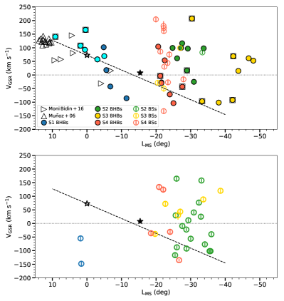
Figure 10: Phase-space distribution of the Magellanic BHB (filled circles) and BS (open circles) stars. The colours are the same as in Figure 9. The dashed line shows the projected LMC’s velocity vector onto the line of sight crossing the LMC halo at $L_{\rm MS}=0\degr$ while the dotted line marks the expected GSR velocity for MW stars. The open and filled stars mark the position of the LMC and SMC, respectively. The top panel shows the BHBs and distant BSs for the four streams, while the bottom panel shows those BS stars with smaller distances, and that most likely belong to the MW halo. Black open triangles correspond to giant stars in the 332 km s^-1 group identified by Muñoz et al. (2006), while the open rightwards-pointing triangles are young stars in the periphery of the LMC detected by Moni Bidin et al. (2017).

Stars from S4 (both BHBs and BSs) appear roughly following the LMC’s halo trend with $V_{\rm GSR}<-50$ km s^-1 at $L_{\rm MS}$ = –20$\degr$ to –30$\degr$. There are also S4 stars with radial velocities $V_{\rm GSR}>0$ km s^-1, reaching up to $V_{\rm GSR}$ = 205 km s^-1 (S4 06), reinforcing the idea that, given their distances and velocities, these stars are possibly coming from the MCs than from the MW. Nonetheless, we can not exclude the possibility that some, plausibly a large fraction, of these stars can actually be part of the MW halo. This is because the kinematic model predictions for the virialised Galactic stellar halo and the Magellanic debris overlap significantly in this region of the sky. At distances beyond 60 kpc, the V_GSR distribution of the MW stellar halo can be described by a Gaussian with a mean at zero and a dispersion of 90 $\pm$ 20 km s^-1 (see Deason et al., 2012). Therefore, in what follows we do not claim an unambiguous detection of Magellanic debris for $L_{\rm MS}<-20^{\circ}$, but rather explore the trends under the assumption that some of the stars in our sample could genuinely come from the Clouds.

Interestingly, there is a group of stars spanning at least 10 deg on the sky (with $L_{\rm BS}$ from –20$\degr$ to –35$\degr$) that show very similar radial velocities, clumped at $V_{\rm GSR}\approx$ 84.0 km s^-1 (including stars from S2, S3 and S4 with $V_{\rm GSR}$ between 50 and 150 km $s^{-1}$). This cold (velocity dispersion of 18.0 km s^-1) group does not seem to be related either to the LMC’s halo velocity trend at this position or to the MW halo. The possible origin of this group is discussed in the following Section.

Figure 11 shows the metallicity distributions for stars belonging to the four different streams that are likely members of the MCs. Stars without EW of Ca measured (too shallow lines) and for which only upper limits in [Fe/H] are estimated are not included in the histograms. The left panel shows the distribution of BHB and BS stars, irrespective of their membership; the middle panel shows the same stars but divided into four subsamples: (i) BHB and (ii) BS stars likely belonging to the LMC, (iii) BHB and (iv) BS stars likely belonging to the SMC based on their measured radial velocities; while the right panel shows the metallicity distribution of LMC and SMC stars (irrespective of their classification as BHB or BS). The LMC/SMC classification is tentative and is based on the comparison with numerical simulations as explained in Section 3.1. The metallicity distribution of the BHB stars shows that the population is metal-poor, with an average [Fe/H] = –1.69 and 1$\sigma$ dispersion of 0.34 dex. The high metallicity of S4 17 and S4 47 can be explained considering they are more likely a BS or an A-type star instead of being a BHB. In fact, Clewley et al. (2002) found that a few A-type or BS stars can be misclassified as BHB stars using the scale-width-shape method if those stars have anomalously high metallicity ([Fe/H] $>$ –0.5). Since S4 17 and S4 47 have very uncertain [Fe/H] values (given their high EW of Ca), no firm conclusions about their classification can be established. For the BS stars, the metallicity distribution tend to be more metal-rich, with a mean metallicity of [Fe/H] = –0.75 and 1$\sigma$ dispersion of 0.36 dex (excluding the four most metal-poor stars, with [Fe/H] < –1.5 dex). The two most metal-rich stars deviates from the group, with [Fe/H] = –0.3 (S4 12) and 0.05 dex (S4 26). It could be possible that this group of stars corresponds to bona-fide (young) main sequence stars, instead of BSs, which occupy the same region in the colour-magnitude diagram and should have similar surface gravity as dwarf stars. The same explanation can be true for the stars classified as BHB/BS (not included in the metallicity distributions shown in Figure 11) which have [Fe/H] up to 0.66 dex (S4 47).

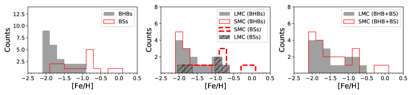
Figure 11: Metallicity distribution of BHB and BS stars in the MCs. Left: [Fe/H] distribution of BHB (grey filled bars) and BS (red unfilled bars) samples, irrespective of their possible association with the LMC or SMC. Middle: Same stars as in the left panel but divided into four subsamples: BHB and BS stars likely belonging to the LMC (grey filled and hatched bars, respectively), BHB (red unfilled bars) and BS (red dashed-line bars) stars likely associated to the SMC. Right: Metallicity distribution for the same stars according to the association to the LMC (grey filled bars) or the SMC (red unfilled bars), irrespective of their stellar classification.

The middle panel in Figure 11 shows the metallicity distribution or the BHB and BS stars that are likely associated with the LMC or SMC separately. Most of the LMC stars (18/5) are BHBs with a mean metallicity [Fe/H] = –1.62 and a 1$\sigma$ dispersion of 0.38 dex, while the BHB and BS stars associated to the SMC have slightly lower mean metallicity, [Fe/H] = –1.77 for BHBs (1$\sigma$ = 0.28 dex) and [Fe/H] = –0.93 for BSs (1$\sigma$ = 0.51 dex). As a whole sample, the mean metallicity of SMC stars is [Fe/H] = –1.37 (1$\sigma$ = 0.58 dex) while for LMC stars is [Fe/H] = –1.49 (1$\sigma$ = 0.47 dex). As it is evident in the right panel of Figure 11, the metallicity distribution of the likely SMC stars tends to be slightly more metal-rich than the distribution of the LMC stars.

Our metallicity estimates are lower compared to the mean (photometrically derived) metallicity using RR Lyrae stars reported by Haschke et al. (2012), who found [Fe/H] = –1.5 and [Fe/H]=–1.70 for the LMC and SMC, respectively. The difference of up to 0.3 dex may be explained by a systematic difference between our method and the light-curve based metallicity, or by the differences in the tracers themselves. Another possible explanation is that this apparent discrepancy could be due to a metallicity gradient as a function of distance from the LMC/SMC centre. As shown in Fig. 4 of Haschke et al. (2012), the mean metallicity of the RR Lyrae stars in the LMC was derived based on the inner 8 kpc of the galaxy, while at distances beyond 10 kpc, the metallicity drops by about 0.25 dex with respect to the stars in the innermost region. Nonetheless, the precision of our metallicity measurements is not good enough to identify unambiguously the cause of this discrepancy.

3.1 Comparison with simulations

Figure 12 compares the phase-space coordinates of our Magellanic BHB and BS stars to the predictions from the simulations of Jethwa et al. (2016). The underlying contours show the density of the LMC and SMC debris particles, from a large suite of simulations corresponding to a sample of 150 proper motion values for the MCs, each containing 1000 tracer particles, for the following galaxy masses: ($M_{\rm MW}$, $M_{\rm LMC}$, $M_{\rm SMC}$) = (75.0, 15.0, 2.0) $\times 10^{10}$ M_⊙. We note that the comparison of our data with the numerical simulations should be taken as illustrative as we do not attempt to match our measurements to the mock debris distributions at hand. According to our preliminary analysis, while the phase-space distribution of the debris is clearly sensitive to the exact LMC/SMC mass ratio adopted as well as the orbital properties of the binary in-fall, some of the trends discussed here remain mostly unchanged. In the top panel, the LMC debris are compared to the stars that appear to follow the LMC’s halo velocity gradient (see Figure 10): more precisely, all S1 stars plus S2 to S4 stars with V${}_{\rm GSR}<0$ km s^-1. As discussed above, even stars located beyond 30 deg from the LMC’s center are located close to the predicted track of the LMC’s debris in phase-space. Moreover, it seems that the more metal-poor S1 BHB stars are following a different path compared to the bulk of the simulations, albeit well inside the region predicted to be occupied by the LMC debris. The slight difference in the behaviour of the S1 stars with different metallicities is curious, however. As Figure 9 demonstrates, the metal-richer S1 stars are on average much closer to the LMC –many appear to coincide with the disc spur described in Mackey et al. (2016) and several are likely to be still bound to the LMC. On the other hand, the metal-poorer members of S1 all lie very far from the LMC, and in fact occupy a very different range of $B_{\rm MS}$, namely $20^{\circ}<B_{\rm MS}<30^{\circ}$ as opposed to $B_{\rm MS}<20^{\circ}$.

The BHB and BS stars with V${}_{\rm GSR}>0$ km s^-1 in our sample appear to be somewhat at odds with the predicted phase-space distribution of the LMC debris based on the Jethwa et al. (2016) simulations. These also do not follow the LMC velocity trend (see Figure 10). Given their mean velocity of $V_{\rm GSR}$ = 95 km s^-1, with a velocity dispersion of $\sim$ 50 km s^-1, it is unlikely that the stars in this subgroup represent a random sample of the MW halo. In fact, we speculate that these are instead a part of the SMC debris also expected to litter this area of the sky (see e.g., Besla et al., 2010; Olsen et al., 2011; Belokurov et al., 2017; Deason et al., 2017). Accordingly, middle and bottom panels of Figure 12 show the results from Jethwa et al. (2016) simulations for the SMC particles. The difference between these two panels is the inclusion (exclusion) of the dynamical friction (DF) exerted by the LMC onto the SMC: middle (bottom) panel shows the prediction from the simulation when it is on (off). Note that in these simulations, the DF of the MW on the MCs is always included. The group of Magellanic BHB and BS stars which have V${}_{\rm GSR}>0$ km s^-1 is overplotted, as well as the LMC’s halo velocity gradient (dashed line) for reference. There appears to be a better match between these “faster” stars and the SMC debris if the LMC-SMC DF is taken into account. Note that the effects of the DF, both from the MW and from the LMC, is the main difference between the simulations of Jethwa et al. (2016) and those carried out by Besla et al. (2010) and Belokurov et al. (2017).

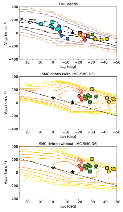
Figure 12: Phase-space distribution for LMC (top) and SMC (middle and bottom) debris, based on the N-body simulations of Jethwa et al. (2016). Middle and bottom panels show the results when the DF by the LMC on the SMC is included and when it is not, respectively. The top panel shows all our Magellanic BHB and BS stars that seem to follow the LMC’s halo velocity trend (dashed line): i.e., all S1 stars and S2, S3 and S4 stars with V${}_{\rm GSR}<$ 0 km s^-1, while middle and bottom panels show BHB and BS stars from S2, S3 and S4 with V${}_{\rm GSR}>$ 0 km s^-1.

Interestingly, the comparison of the three panels of Figure  12 shows that at negative $L_{\rm MS}$, the SMC debris encompasses a broader range of radial velocities as compared to the LMC particles. In fact, the cloud of the SMC particles is sufficiently broad to accommodate the stars with both negative and positive $V_{\rm GSR}$. Superficially, this is unusual given that the tidal stream width typically correlates with the progenitor’s mass (Erkal et al., 2016) and the SMC is at least 5-10 times lighter than the LMC. We suspect that the phase-space distribution of the SMC particle has been affected by the interaction with the LMC. To look for signs of the LMC influence on the SMC debris, we split the SMC particles into three groups according to the distance of their minimal approach to the LMC, min$(D_{\rm LMC})$. The distribution of the approach distances for all particles is shown in the top panel of Figure 13. A large number of the SMC particles in the simulation have passed as close as $\lesssim$ 10 kpc (the peak of the distribution) from the LMC. A considerable fraction of the particles has reached a minimum distance between 25 and 50 kpc. There remains, however, a significant number of particles that interacted very weakly with the LMC, never approaching closer than 50 kpc.

The middle and bottom panels of Figure 13 show the distributions of the three groups of SMC particles described above in phase-space. Particles that have sustained the strongest perturbation from the LMC, coming as close as 25 kpc to it, lie predominantly at positive $L_{\rm MS}$ (red contours). Unsurprisingly, these are also the closest to the LMC on the sky. At negative $L_{\rm MS}$, the velocity distribution bifurcates into two sequences: one corresponding to the stars with min$(D_{\rm LMC})>50$ kpc (blue), located at negative radial velocities, and the one corresponding to the stars with $25<$ min$(D_{\rm LMC})[{\rm kpc}]<50$ (green) with positive $V_{\rm GSR}$. Note that these two sequences are visible regardless of whether the LMC-SMC DF is taken into account or not. Alternatively, the min$(D_{\rm LMC})$ parameter can be considered as a proxy for the “unbinding” time –the epoch at which the SMC stars have been fully stripped, i.e. stopped being influenced by their progenitor galaxy and started orbiting the MW-LMC system.

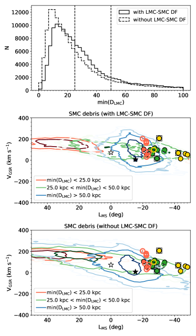
Figure 13: Top panel: Distribution of minimum distance to the LMC for 1000 particles, in 150 realizations of proper motion values from the simulations of Jethwa et al. (2016), for those including and not including the DF effect of the LMC on the SMC debris particles (solid and dashed lines, respectively). Middle and bottom panels: contour density of SMC debris particles for simulations with and without LMC-SMC DF included. Red, green and blue contours correspond to particles which reach a minimum distance to the LMC, at a given point of their orbits, of less than 25 kpc, between 25 to 50 kpc and greater than 50 kpc, respectively.

4 Discussion and Conclusions

We have used FORS2 on the VLT to obtain medium-resolution spectroscopy of 104 candidate A-type stars in the vicinity of the MCs. These were selected to lie along the four candidate streams announced in Belokurov & Koposov (2016). Of these, 25 objects turned out to be contaminants, predominantly QSO, and WDs. The spectra of the remaining 79 stars show prominent Balmer series absorption lines in the wavelength range of 3600 - 5110 Å. We model the observed spectra with a combination of Sérsic profiles for the absorption and a fifth-degree polynomial for the continuum (see Figure 1). Using the shapes of the Balmer lines we devise a classification scheme to separate the BHB stars from BSs, which we test on a large sample of high quality spectra of similar resolution, provided by the SDSS (see Figure 2). According to our classification, 24 stars are of BHB type, 45 are BSs and 10 have uncertain classification (see Figure 3). All of our BHB stars lie beyond 35 kpc from the Sun, and therefore we consider the 15 BS stars with Galactocentric distances larger than 35 kpc as part of the final sample of stars of likely Magellanic origin. Additionally, we use Ca II K line at 3933 Å to estimate the stellar metallicity. We devise an empirical calibration based on the equivalent width values available for a sample of BHBs and BSs with available SDSS spectroscopic data (see Figures 7 and 8).

Stars classified as BHBs and BSs show different behavior in the phase-space spanned by the line-of-sight velocity $V_{\rm GSR}$ and the MS longitude $L_{\rm MS}$ (Figure 10). Velocities of the BS stars appear consistent with a Gaussian distribution centered on $V_{\rm GSR}=0$ and having a dispersion of 88 km s^-1. This can be contrasted with the distribution of the BHB stars, many of which avoid $V_{\rm GSR}=0$ and instead line up in several narrow sequences at positive and negative $V_{\rm GSR}$. Such obvious difference in the phase-space distribution provides further support for our BHB/BS classification.

Of the four candidate streams presented in Belokurov & Koposov (2016), only two, S1 and S2, appear kinematically distinct. The S2 stream not only has a relatively small velocity dispersion of 15.0 km s^-1 (excluding the S2 star with $V_{\rm GSR}$ < 0), it also has narrow Ca K equivalent width –and thus metallicity– distribution (see Figure 6). Curiously, the S1 stars with the highest metallicity are also the ones closest to the LMC’s disc (see Figure 9). In fact, several of these appear to overlap with the spur detected by Mackey et al. (2016). It is not therefore impossible that rather than metal-rich BHBs (some of) these could instead be bona-fide Young Main Sequence stars. The remaining, metal-poor S1 stars follow a different phase-space track, reaching as far as $\sim 30^{\circ}$ north of the LMC’s center. Therefore, we conjecture that the S1 stars considered here actually sample two different structures in the northern side of the LMC. Comparing the velocity and the metallicity distributions of the stars in S1 and S2, we conclude that S2 –metal poor and cold– is the best candidate to date for a tidal stream from a low-mass system accreted by the LMC.

Looking at all of the stars in our “Magellanic” sample, i.e. 24 BHBs, 15 BSs and 10 BHB/BSs, we note two clear trends of the radial velocity as a function of MS longitude. First, most of the S1 stars and a large fraction of S3 and S4 ones follow a clear velocity trend where $V_{\rm GSR}$ steadily decreases with angular distance from the LMC (see dashed line in Figure 10). Interestingly, it is impossible to distinguish between the stars still bound to the LMC and the stars in its tidal tail based on their $(V_{\rm GSR},L_{\rm MS})$ position. This is because the projection of the LMC’s space velocity onto the line of sight and the centroid of the tidal debris coincide in phase-space (see Figure 12). Regardless of whether these stars are still bound to or recently stripped from the LMC, these objects (marked with “M1” in Table 1) are probably of Magellanic origin.

We also investigate whether any of the stars in our sample could have originated in the SMC. According to Figure 12, all of them could! Even for lower (1.0 $\times 10^{10}M_{\odot}$) and higher (3.0, 4.0 $\times 10^{10}M_{\odot}$) SMC masses, the velocity trend is compatible with the group of stars at high GSR velocities located between $L_{\rm MS}=-20\degr$ to $-50$°(P. Jethwa, private communication). Note that, for a large number of stars, it is impossible to identify whether they were (are) part of the LMC or the SMC based on the data in hand. Nonetheless, there exists a group of stars with $V_{\rm GSR}>0$ and $L_{\rm MS}<-20^{\circ}$ with velocities significantly higher compared to what is predicted for the LMC particles at a given MS longitude (marked with “M2” in Table 1). However, the kinematics of these stars can be easily explained if they were stripped from the SMC. As Figure 13 illustrates, at negative $L_{\rm MS}$ there exists a bifurcation in the velocity distribution of the SMC particles. Stars populate different branches of the velocity bifurcation according to the distance of the closest approach to the Large Cloud. This effect can plausibly be explained by two phenomena. First, the minimal distance to the LMC likely correlates with the time of unbinding of a particle from the SMC. Thus, the velocity bifurcation is the natural consequence of the orbital evolution of the particles in a combined potential of the LMC+MW. A second, related explanation is possible where a certain distance exists within which the LMC influences the orbits of the SMC debris enough to elevate them to a higher velocity.

Note that at large angular distances from the LMC, given the data in hand, it is not possible to identify securely which stars were stripped from the Clouds and which belong to the virialised MW halo. Therefore, while we confirm the Magellanic origin for S1 and S2 stars, for association between the Clouds and S3 and S4 stars should be considered as a speculation, which if proven can shed light onto the history of interaction between the LMC and SMC and the Milky Way. We look forward to testing this hypothesis using the astrometric information from the Gaia satellite.

References

- Ahn et al. (2012) Ahn C. P., et al., 2012, ApJS, 203, 21
- Alves (2004) Alves D. R., 2004, ApJ, 601, L151
- Balbinot et al. (2015) Balbinot E., et al., 2015, MNRAS, 449, 1129
- Bechtol et al. (2015) Bechtol K., et al., 2015, ApJ, 807, 50
- Beers (1990) Beers T. C., 1990, AJ, 99, 323
- Bell et al. (2010) Bell E. F., Xue X. X., Rix H.-W., Ruhland C., Hogg D. W., 2010, AJ, 140, 1850
- Belokurov & Koposov (2016) Belokurov V., Koposov S. E., 2016, MNRAS, 456, 602
- Belokurov et al. (2017) Belokurov V., Erkal D., Deason A. J., Koposov S. E., De Angeli F., Evans D. W., Fraternali F., Mackey D., 2017, MNRAS, 466, 4711
- Besla et al. (2010) Besla G., Kallivayalil N., Hernquist L., van der Marel R. P., Cox T. J., Kereš D., 2010, ApJ, 721, L97
- Besla et al. (2012) Besla G., Kallivayalil N., Hernquist L., van der Marel R. P., Cox T. J., Kereš D., 2012, MNRAS, 421, 2109
- Besla et al. (2013) Besla G., Hernquist L., Loeb A., 2013, MNRAS, 428, 2342
- Bland-Hawthorn & Gerhard (2016) Bland-Hawthorn J., Gerhard O., 2016, ARA&A, 54, 529
- Brown et al. (2006) Brown W. R., Geller M. J., Kenyon S. J., Kurtz M. J., 2006, ApJ, 647, 303
- Busha et al. (2011) Busha M. T., Marshall P. J., Wechsler R. H., Klypin A., Primack J., 2011, ApJ, 743, 40
- Clewley et al. (2002) Clewley L., Warren S. J., Hewett P. C., Norris J. E., Peterson R. C., Evans N. W., 2002, MNRAS, 337, 87
- D’Onghia & Fox (2016) D’Onghia E., Fox A. J., 2016, ARA&A, 54, 363
- Deason et al. (2011) Deason A. J., Belokurov V., Evans N. W., 2011, MNRAS, 416, 2903
- Deason et al. (2012) Deason A. J., et al., 2012, MNRAS, 425, 2840
- Deason et al. (2017) Deason A. J., Belokurov V., Erkal D., Koposov S. E., Mackey D., 2017, MNRAS, 467, 2636
- Diaz & Bekki (2011) Diaz J., Bekki K., 2011, MNRAS, 413, 2015
- Diaz & Bekki (2012) Diaz J. D., Bekki K., 2012, ApJ, 750, 36
- Diehl et al. (2014) Diehl H. T., et al., 2014, in Observatory Operations: Strategies, Processes, and Systems V. p. 91490V, doi:10.1117/12.2056982
- Drlica-Wagner et al. (2015) Drlica-Wagner A., et al., 2015, ApJ, 813, 109
- Drlica-Wagner et al. (2016) Drlica-Wagner A., et al., 2016, ApJ, 833, L5
- Erkal et al. (2016) Erkal D., Sanders J. L., Belokurov V., 2016, MNRAS, 461, 1590
- Feast (1968) Feast M. W., 1968, MNRAS, 140, 345
- Fritz et al. (2018b) Fritz T. K., Carrera R., Battaglia G., 2018b, preprint, (arXiv:1805.07350)
- Fritz et al. (2018a) Fritz T. K., Battaglia G., Pawlowski M. S., Kallivayalil N., van der Marel R., Sohn T. S., Brook C., Besla G., 2018a, preprint, (arXiv:1805.00908)
- Fukushima et al. (2018) Fukushima T., et al., 2018, PASJ, 70, 69
- Gaia Collaboration et al. (2016) Gaia Collaboration et al., 2016, A&A, 595, A2
- Gaia Collaboration et al. (2018) Gaia Collaboration et al., 2018, A&A, 616, A12
- Hammer et al. (2015) Hammer F., Yang Y. B., Flores H., Puech M., Fouquet S., 2015, ApJ, 813, 110
- Haschke et al. (2012) Haschke R., Grebel E. K., Duffau S., Jin S., 2012, AJ, 143, 48
- Irwin (1991) Irwin M. J., 1991, in Haynes R., Milne D., eds, IAU Symposium Vol. 148, The Magellanic Clouds. p. 453
- Jester et al. (2005) Jester S., et al., 2005, AJ, 130, 873
- Jethwa et al. (2016) Jethwa P., Erkal D., Belokurov V., 2016, MNRAS, 461, 2212
- Kallivayalil et al. (2006) Kallivayalil N., van der Marel R. P., Alcock C., Axelrod T., Cook K. H., Drake A. J., Geha M., 2006, ApJ, 638, 772
- Kallivayalil et al. (2013) Kallivayalil N., van der Marel R. P., Besla G., Anderson J., Alcock C., 2013, ApJ, 764, 161
- Kallivayalil et al. (2018) Kallivayalil N., et al., 2018, preprint, (arXiv:1805.01448)
- Kim & Jerjen (2015) Kim D., Jerjen H., 2015, ApJ, 808, L39
- Kinman & Brown (2011) Kinman T. D., Brown W. R., 2011, AJ, 141, 168
- Kinman et al. (1991) Kinman T. D., Stryker L. L., Hesser J. E., Graham J. A., Walker A. R., Hazen M. L., Nemec J. M., 1991, PASP, 103, 1279
- Kinman et al. (1994) Kinman T. D., Suntzeff N. B., Kraft R. P., 1994, AJ, 108, 1722
- Koposov et al. (2015) Koposov S. E., et al., 2015, ApJ, 811, 62
- Lee et al. (2008) Lee Y. S., et al., 2008, AJ, 136, 2022
- Mackey et al. (2016) Mackey A. D., Koposov S. E., Erkal D., Belokurov V., Da Costa G. S., Gómez F. A., 2016, MNRAS, 459, 239
- Mackey et al. (2018) Mackey D., Koposov S., Da Costa G., Belokurov V., Erkal D., Kuzma P., 2018, ApJ, 858, L21
- Majewski et al. (2009) Majewski S. R., Nidever D. L., Muñoz R. R., Patterson R. J., Kunkel W. E., Carlin J. L., 2009, in Van Loon J. T., Oliveira J. M., eds, IAU Symposium Vol. 256, The Magellanic System: Stars, Gas, and Galaxies. pp 51–56, doi:10.1017/S1743921308028251
- Minniti et al. (2003) Minniti D., Borissova J., Rejkuba M., Alves D. R., Cook K. H., Freeman K. C., 2003, Science, 301, 1508
- Moni Bidin et al. (2017) Moni Bidin C., Casetti-Dinescu D. I., Girard T. M., Zhang L., Méndez R. A., Vieira K., Korchagin V. I., van Altena W. F., 2017, MNRAS, 466, 3077
- Muñoz et al. (2006) Muñoz R. R., et al., 2006, ApJ, 649, 201
- Murga et al. (2015) Murga M., Zhu G., Ménard B., Lan T.-W., 2015, MNRAS, 452, 511
- Nidever et al. (2008) Nidever D. L., Majewski S. R., Butler Burton W., 2008, ApJ, 679, 432
- Olsen et al. (2011) Olsen K. A. G., Zaritsky D., Blum R. D., Boyer M. L., Gordon K. D., 2011, ApJ, 737, 29
- Pace & Li (2018) Pace A. B., Li T. S., 2018, preprint, (arXiv:1806.02345)
- Pedregosa et al. (2011) Pedregosa F., et al., 2011, Journal of Machine Learning Research, 12, 2825
- Pieres et al. (2017) Pieres A., et al., 2017, MNRAS, 468, 1349
- Rodgers et al. (1981) Rodgers A. W., Harding P., Sadler E., 1981, ApJ, 244, 912
- Saha et al. (2010) Saha A., et al., 2010, AJ, 140, 1719
- Schlafly & Finkbeiner (2011) Schlafly E. F., Finkbeiner D. P., 2011, ApJ, 737, 103
- Sérsic (1968) Sérsic J. L., 1968, Atlas de galaxias australes (Observatorio Astronómico, Universidad Nacional de Córdoba, Córdoba)
- Simon (2018) Simon J. D., 2018, ApJ, 863, 89
- Sirko et al. (2004) Sirko E., et al., 2004, AJ, 127, 899
- Torrealba et al. (2018) Torrealba G., et al., 2018, MNRAS, 475, 5085
- Vickers et al. (2012) Vickers J. J., Grebel E. K., Huxor A. P., 2012, AJ, 143, 86
- Wilhelm et al. (1999) Wilhelm R., Beers T. C., Gray R. O., 1999, AJ, 117, 2308
- Xue et al. (2008) Xue X. X., et al., 2008, ApJ, 684, 1143
- Xue et al. (2015) Xue X.-X., Rix H.-W., Ma Z., Morrison H., Bovy J., Sesar B., Janesh W., 2015, ApJ, 809, 144