An Adversarial Approach for Explainable AI in Intrusion Detection Systems

Abstract

Despite the growing popularity of modern machine learning techniques (e.g. Deep Neural Networks) in cyber-security applications, most of these models are perceived as a black-box for the user. Adversarial machine learning offers an approach to increase our understanding of these models. In this paper we present an approach to generate explanations for incorrect classifications made by data-driven Intrusion Detection Systems (IDSs) An adversarial approach is used to find the minimum modifications (of the input features) required to correctly classify a given set of misclassified samples. The magnitude of such modifications is used to visualize the most relevant features that explain the reason for the misclassification. The presented methodology generated satisfactory explanations that describe the reasoning behind the mis-classifications, with descriptions that match expert knowledge. The advantages of the presented methodology are: 1) applicable to any classifier with defined gradients. 2) does not require any modification of the classifier model. 3) can be extended to perform further diagnosis (e.g. vulnerability assessment) and gain further understanding of the system. Experimental evaluation was conducted on the NSL-KDD99 benchmark dataset using Linear and Multilayer perceptron classifiers. The results are shown using intuitive visualizations in order to improve the interpretability of the results.

I Introduction

The increasing incorporation of Cyber-based methodologies for monitoring and control of physical systems has made critical infrastructure vulnerable to various cyber-attacks such as: interception, removal or replacement of information, penetration of unauthorized users and viruses [1] [2] [3] [4]. Intrusion detection systems (IDSs) are an essential tool to detect such malicious attacks [5].

Extendibility and adaptability are essential requirements for an IDS [6]. Every day, new strains of Cyber-attacks are created with the objective of deceiving these systems. As a result, machine learning and data-driven intrusion detection systems are increasingly being used in cyber-security applications [6]. Machine learning techniques such as deep neural networks have been successfully used in IDSs [6] [7]. However, these techniques often work as a black-box model for the user. [8] [7].

Figure 1: Explainable AI [9] is concerned with designing of interfaces that help users to understand the decisions made by a trained machine learning model.

Figure 2: Overview of the presented explainable interface. The approach provides explanations for misclassified samples. An adversarial approach is followed to modify the misclassified samples until the model assigns the correct class. This approach provides a mechanism to understand the decision boundaries of the classifier.

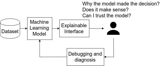
With machine learning being increasingly applied in the operation of critical systems, understanding the reason behind the decisions made by a model has become a common requirement to the point that governments are starting to include it into legislation [10] [11]. Recent developments in the machine learning community have been focused in the development of methods which are more interpretable for the users. Explainable AI (Figure 1) [8] makes use of visualizations and natural language descriptions to explain the reasoning behind the decisions made by the machine learning model.

It is crucial that the inner workings of data-driven models are transparent for the engineers designing IDSs. Decisions presented by explainable models can be easily interpreted by a human, simplifying the process of knowledge discovery. Explainable approaches help on diagnosing, debugging, and understanding the decisions made by the model, ultimately increasing the trust on the data-driven IDS.

In the case of data-driven IDS, when the model is presented with new attacks where data is not available, the model might mis-classify an attack as normal, leading to a breach in the system. Understanding the reasons behind the misclassification of particular samples is the first step for debugging and diagnosing the system. Providing clear explanations for the cause of misclassification is essential to decide which steps to follow in order to prevent future attacks.

In this paper, we present an explainable AI interface for diagnosing data-driven IDSs. We present a methodology to explain incorrect classifications made by the model following an adversarial approach.

Although adversarial machine learning is usually used to deceive the classifier, in this paper we use it to generate explanations by finding the minimum modifications required in order to correctly classify the misclassified samples. The difference between the original and modified samples provide information of the relevant features responsible for the misclassification. We show the explanations provide satisfactory insights behind the reasoning made by the data-driven models, being congruent with the expert knowledge of the task.

The rest of the paper is organized as follows: Section II presents an overview of adversarial machine learning; Section III describes the presented methodology for explainable IDS systems. Section IV describes the experimental results carried out using the NSL-KDD99 intrusion detection benchmark dataset. Section V concludes the paper.

II Adversarial Machine Learning

Adversarial machine learning has been extensively used in cyber-security research to find vulnerabilities in data-driven models [12] [13] [14] [15] [16] [17]. Recently, there has been an increasing interest on adversarial samples given the susceptibility of Deep Learning models to these type of attacks [18] [19].

Adversarial samples are samples crafted in order to change the output of a model by making small modifications into a reference (usually real) sample [18]. These samples are used to detect blind spots on ML algorithms.

Adversarial samples are crafted from an attacker perspective to evade detection, confuse the classifier [18], degrade performance [20] and/or gain information about the model or the dataset used to train the model [17]. Adversarial samples are also useful from a defender point of view given that they can be used to perform vulnerability assessment [16], study the robustness against noise, improve generalization and debug the machine learning model [20].

In general, the problem of crafting an adversarial sample is stated as follows [17]:

$$\max_{\hat{{\boldsymbol{x}}}}\quad \mathcal{L}({\hat{{\boldsymbol{x}}}})-\Omega({\hat{{\boldsymbol{x}}}})$$ (1)

$$s.t.\quad {\hat{{\boldsymbol{x}}}}\in\phi({\boldsymbol{x}})$$

where:

• $\mathcal{L}({\boldsymbol{x}})$ measures the impact of the adversarial sample in the model,

• $\Omega({\boldsymbol{x}})$ measures the capability of the defender to detect the adversarial sample.

• ${\hat{{\boldsymbol{x}}}}\in\phi({\boldsymbol{x}})$ ensures the crafted sample ${\hat{{\boldsymbol{x}}}}$ is inside the domain of valid inputs. It also represents the capabilities of the adversary.

The objective of Eq. (1) can be interpreted as crafting an attack point ${\hat{{\boldsymbol{x}}}}$ that maximizes the impact of the attack, while minimizing the chances of the attack to be detected. The definition of $\mathcal{L}({\boldsymbol{x}})$ will depend on the intent of the attack and the available information about the model under attack. For example: 1) $\mathcal{L}({\boldsymbol{x}})$ can be a function that measures the difference between a target class ${\hat{{\boldsymbol{y}}}}$ and the output from the model; 2) $\Omega({\boldsymbol{x}})$ measures the discrepancy between the reference and the modified sample ${\hat{{\boldsymbol{x}}}}$

In this paper, instead of deceiving the classifier, we use Equation 1 to find the minimum number of modifications needed to correctly classify a misclassified sample. The methodology is described in detail in section III.

III Explaining misclassifications using adversarial machine learning

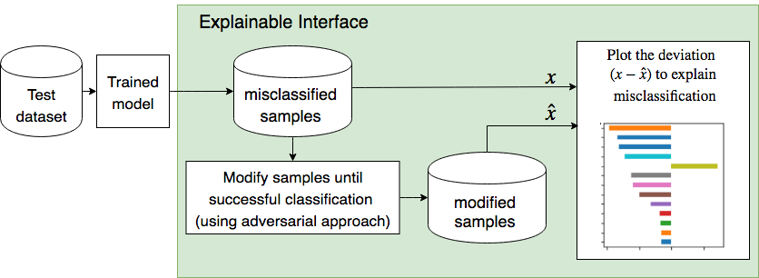
In this paper we are interested in generating explanations for incorrect estimations made by a trained classifier. Figure 2 presents an overview of the presented explainable interface. The presented methodology modifies a set of misclassified samples until they are correctly classified. The modifications are made following an adversarial approach: finding the minimum modifications required to change the output of the model. The difference between the modified samples and the original real samples is used to explain the output from the classifier, illustrating the most relevant features that lead to the misclassification.

In the following sections we explain in detail each component of the presented explainable interface.

III-A Data-driven classifier

The classifier ${p\left(y=k|{\boldsymbol{x}},w\right)}$ estimates the probability of a given sample ${\boldsymbol{x}}$ to belong to class $k$. The classifier is parameterized by a set of parameters $w$ that are learned from data. Learning is performed using standard supervised learning. Given a training dataset ${\cal D}={\left\{({\boldsymbol{x}}^{(i)},{\boldsymbol{y}}^{(i)})\right\}}_{i}^{M}$ of $M$ samples, the parameters $w$ of the model are obtained by minimizing the cross-entropy:

$$w^{*}=\operatorname*{arg\,min}_{w}\sum_{i}^{M}{H\left({\boldsymbol{y}}^{(i)},{p\left({\boldsymbol{y}}|{\boldsymbol{x}}^{(i)},w\right)}\right)}$$

where ${\boldsymbol{y}}^{(i)}$ is a one-hot encoding representation of the class:

$${\boldsymbol{y}}_{i}=\begin{cases}1\quad\text{if ${\boldsymbol{x}}^{(i)}\in$ class $i$}\\ 0\quad\text{otherwise}\end{cases}$$

Depending on the complexity of the model ${p\left({\boldsymbol{y}}|{\boldsymbol{x}},w\right)}$ and the dataset ${\cal D}$, the model may misclassify some of the samples. We are interested on provide explanations for these incorrect estimations.

III-B Modifying misclassified samples

In this paper, instead of deceiving the classifier, we make use of adversarial machine learning to understand why some of the samples are being mis-classified. The idea of this approach is that adversarial machine learning can help us to understand the decision boundaries of the learned model.

The objective is to find the minimum modifications needed in order to change the output of the classifier for a real sample . This is achieved by finding an adversarial sample ${\hat{{\boldsymbol{x}}}}$ that is classified as ${\hat{{\boldsymbol{y}}}}$ while minimizing the distance between the real sample () and the modified sample ${\hat{{\boldsymbol{x}}}}$:

$$\min_{{\hat{{\boldsymbol{x}}}}}\quad \left(\hat{{\boldsymbol{x}}}-{{\boldsymbol{x}}_{0}}\right)^{T}{\boldsymbol{Q}}\left(\hat{{\boldsymbol{x}}}-{{\boldsymbol{x}}_{0}}\right)$$ (2)

s.t $$\operatorname{argmax}_{k}{{p\left({\boldsymbol{y}}=k|\hat{{\boldsymbol{x}}},w\right)}}={\hat{{\boldsymbol{y}}}}$$ (3)

$${\boldsymbol{x}}_{\min}\preceq{\hat{{\boldsymbol{x}}}}\preceq{\boldsymbol{x}}_{\max}$$

where ${\boldsymbol{Q}}$ is a symmetric positive definite matrix, that allows the user to specify a weight in the quadratic difference metric.

The program in Equation 2 can serve multiple purposes depending on how and ${\hat{{\boldsymbol{y}}}}$ are specified. For the purpose of explaining incorrect classifications, in this paper, represents the real misclassified samples that serve as a reference for the modified samples ${\hat{{\boldsymbol{x}}}}$. Furthermore, the value of ${\hat{{\boldsymbol{y}}}}$ is set to the correct class of . In this way, the program (2) finds a modified sample ${\hat{{\boldsymbol{x}}}}$ that is as close as possible to the real misclassified sample , while being correctly classified by the model as ${\hat{{\boldsymbol{y}}}}$.

We constrain the sample ${\hat{{\boldsymbol{x}}}}$ to be inside the bounds $({\boldsymbol{x}}_{min},{\boldsymbol{x}}_{max})$. These bounds are extracted from the maximum and minimum values found in the training dataset. This constraint ensures that the adversarial example is inside the domain of the data distribution.

The class ${\hat{{\boldsymbol{y}}}}$ of the adversarial sample is specified by the user. Note that ${\boldsymbol{y}}\neq{\hat{{\boldsymbol{y}}}}$, i.e. the class of the real sample is different from the class of the adversarial sample.

The optimization problem in Eq. 2 provides a clear objective to solve. However, the problem as stated in Eq. 2 is not straightforward to solve using available deep-learning optimization frameworks. In order to simplify the implementation, we modify the way the constraints are satisfied by moving the constraint in Eq. 3 into the objective function:

$$\min_{{\hat{{\boldsymbol{x}}}}}\quad H({\hat{{\boldsymbol{y}}}},{p\left({\boldsymbol{y}}|\hat{{\boldsymbol{x}}},w\right)})\alpha{\boldsymbol{I}}_{({\hat{{\boldsymbol{x}}}},{\hat{{\boldsymbol{y}}}})}$$ (4)

$$\quad+\left(\hat{{\boldsymbol{x}}}-{{\boldsymbol{x}}_{0}}\right)^{T}{\boldsymbol{Q}}\left(\hat{{\boldsymbol{x}}}-{{\boldsymbol{x}}_{0}}\right)$$

s.t $${\boldsymbol{x}}_{\min}\preceq{\hat{{\boldsymbol{x}}}}\preceq{\boldsymbol{x}}_{\max}$$

where:

• $(,{\boldsymbol{y}})$ is a reference sample from the dataset

• ${\hat{{\boldsymbol{x}}}}$ is the modified version of that makes the estimation of the class change from ${\boldsymbol{y}}$ to the target ${\hat{{\boldsymbol{y}}}}$

• $H({\hat{{\boldsymbol{y}}}},{p\left({\boldsymbol{y}}|\hat{{\boldsymbol{x}}},w\right)})$ is the cross-entropy between the estimated adversarial sample class ${p\left({\boldsymbol{y}}|\hat{{\boldsymbol{x}}},w\right)}$ and the target class ${\hat{{\boldsymbol{y}}}}$

• ${\boldsymbol{I}}_{({\hat{{\boldsymbol{x}}}},{\hat{{\boldsymbol{y}}}})}$ is an indicator function that specifies whether the adversarial sample ${\hat{{\boldsymbol{x}}}}$ is being classified as ${\hat{{\boldsymbol{y}}}}$

  $${\boldsymbol{I}}_{({\hat{{\boldsymbol{x}}}},{\hat{{\boldsymbol{y}}}})}=\begin{cases}0\quad\text{if $\operatorname{argmax}_{k}{p\left({\boldsymbol{y}}=k|\hat{{\boldsymbol{x}}},w\right)}={\hat{{\boldsymbol{y}}}}$}\\ 1\quad\text{otherwise}\end{cases}$$

  This function provides a mechanism to stop the modifications once the sample ${\hat{{\boldsymbol{x}}}}$ is classified as ${\hat{{\boldsymbol{y}}}}$. We assume this function is not continuous, hence, the gradients with respect the inputs are not required.

• $\alpha$ is a scale factor that can be used to weight the contribution of the cross-entropy $H$ to the objective loss.

The problem stated in Eq. 4 can be seen as an instance of the adversarial problem stated in Eq. 1, where the cross-entropy $H$ represents the effectiveness ($\mathcal{L}$) of the modifications while the quadratic difference represents the discrepancy ($\Omega$) between and ${\hat{{\boldsymbol{x}}}}$.

(a) misclassified samples

(b) misclassified and modified samples ${\hat{{\boldsymbol{x}}}}$

Figure 3: t-SNE visualization of misclassified samples and corresponding modified samples for the MLP classifier. The legend shows the class to which the misclassified samples belong to. The axes correspond to an embedded 2D representation of the samples. The figure shows there is no clear distinction between the misclassified real samples and the modified samples ${\hat{{\boldsymbol{x}}}}$, demonstrating that small modifications can be used to change the output of the classifier.

III-C Explaining incorrect estimations

We used the adversarial approach stated in Eq. 4, to generate an explanation for incorrect classification. Using a set of misclassified samples as reference, we use Eq. 4 to find the minimum modifications needed to correctly classify the samples. We use as target ${\hat{{\boldsymbol{y}}}}$ the real class of the samples.

The explanations are generated by visualizing the difference $(-{\hat{{\boldsymbol{x}}}})$ between the misclassified samples and the modified samples ${\hat{{\boldsymbol{x}}}}$. This difference shows the deviation of the real features from what the model considers as the target class ${\hat{{\boldsymbol{y}}}}$.

The explanations can be generated for individual samples or for a set of misclassified samples. We used the average deviation $(-{\hat{{\boldsymbol{x}}}})$ to present the explanations for a set of misclassified samples.

IV Experiments and Results

IV-A Dataset

For experimental evaluation, we used the NSL-KDD intrusion detection dataset [21]. The NSL-KDD dataset is a revised version of the KDD99 dataset [22], a widely used benchmark dataset used for intrusion detection algorithms. The NSL-KDD dataset removes redundant and duplicate records found in the KDD99 dataset, alleviating some of the problems of the KDD99 dataset mentioned in [21].

The NSL-KDD consists of a series of aggregated records extracted from a packet analyzer log. Besides normal communications, the dataset contains records of attacks that fall in four main categories: DOS, R2L, U2R and proving. For our experiments, we only considered normal, DOS and probe classes.

The dataset consists of 124926 training samples and 16557 testing samples. We used the same split provided by the authors of the dataset. To alleviate the effects of the unbalanced distribution of the samples over the classes, we trained the models extracting mini-batches with an equal ratio of samples from each class. Samples were extracted with replacement. A detailed description of the dataset features can be found in [23].

The dataset samples were normalized in order to make the quadratic distance metric in Equation 4 invariant to the features scales. We used the mean and standard deviation of the training dataset for normalization:

$${\boldsymbol{x}}^{(i)}\leftarrow\dfrac{{\boldsymbol{x}}^{(i)}-{\text{MEAN}\left({\left\{{\boldsymbol{x}}|{\boldsymbol{x}}\in{\cal D}\right\}}\right)}}{{\text{STD}\left({\left\{{\boldsymbol{x}}|{\boldsymbol{x}}\in{\cal D}\right\}}\right)}}$$

IV-B Classifiers

One of the advantages of the methodology presented in this paper is that it works for any classifier which has a defined gradient $\nabla_{{\boldsymbol{x}}}H$ of the cross-entropy loss with respect to the inputs.

For the experimental section, we used the following data-driven models: 1) a linear classifier, and 2) a Multi Layer Perceptron (MLP) classifier with ReLU activation function. We used weight decay (L2 norm) and early-stopping regularization for training both models.

Table I shows the accuracy achieved with the linear and the MLP classifiers. We can see that the MLP classifier provides higher accuracy in the training and testing datasets.

TABLE I: Accuracy of Classifiers

classifier	train	test
Linear	0.957	0.936
MLP	0.995	0.955

IV-C Modified misclassified samples

We used t-SNE [24] to visualize the misclassified samples () and the modified/corrected samples (${\hat{{\boldsymbol{x}}}}$) found using Equation 4. t-SNE is a dimensionality reduction technique commonly used to visualize high-dimensional datasets.

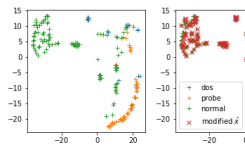
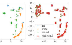
Figure 3 shows the visualization of the misclassified samples and the corresponding modified samples ${\hat{{\boldsymbol{x}}}}$ using t-SNE. This figure shows the effectiveness of the presented methodology to find the minimum modifications needed to correct the output of the classifier. No visual difference in the visualization can be observed between the real and the modified samples. The modified samples ${\hat{{\boldsymbol{x}}}}$ are close enough to the real samples that the modified samples occlude the real samples in Figure 3b.

IV-D Explaining incorrect estimations

(a) Normal samples misclassified as DOS using Linear model

(b) Normal samples misclassified as DOS using MLP model

Figure 4: Explanation for Normal samples being misclassified as DOS using the difference between real samples and modified samples ${\hat{{\boldsymbol{x}}}}$.

Figure 5: Comparison of duration feature between (Normal samples misclassified as DOS) and ${\hat{{\boldsymbol{x}}}}$ (modified samples). The model considers connections with zero duration suspicious. The modified samples have an increased duration in order to correctly classify the samples as Normal.

(a) DOS samples misclassified as Normal using Linear model

(b) DOS samples misclassified as Normal using MLP model

Figure 6: Explanation for DOS samples being misclassified as Normal using the difference between real samples and modified samples ${\hat{{\boldsymbol{x}}}}$.

(a) Deviation for continuous features

(b) Comparison of categorical features distributions

Figure 7: Explanation for Normal samples mis-classified as DOS while taking into account categorical features (MLP model).

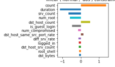
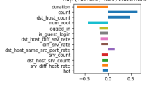
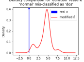
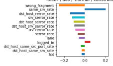
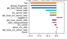
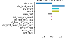
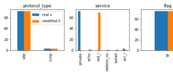
Figure 4 shows the generated explanation for Normal samples being incorrectly classified as DOS. Figure 4a shows the explanations for the Linear model while Figure 4b shows the explanations for the MLP model.

We observed that the explanations for both models provide similar qualitative explanations. Figures 4a and 4b can be naturally interpreted as follows:

Normal samples were mis-classified as DOS because:

• high number of connections to the same host (count) and to the same destination address (dst_host_count)

• low connection duration (duration)

• low number of operations performed as root in the connection (num_root)

• low percentage of samples have successfully logged in (logged_in, is_guest_login)

• high percentage of connections originated from the same source port (dst_host_same_src_port_rate)

• low percentage of connections directed to different services (diff_srv_rate)

• low number of connections were directed to the same destination port (dst_host_srv_count)

Figures 4a and 4b that a high number of connections with low duration and low login success rate is responsible for misclassifying Normal samples as DOS. These attributes are clearly suspicious and match what a human expert would consider as typical behavior of a DOS attack, providing a satisfactory explanation for the incorrect classification.

A more detailed view of the difference between the duration of real () and modified (${\hat{{\boldsymbol{x}}}}$) samples is presented in Figure 5. This figure shows that all misclassified Normal samples had connections with a duration of zero seconds, which the classifier considers suspicious for a Normal behavior.

The graphs also provide a natural way to extract knowledge and understand the concepts learned by the model. For example, figures 4a and 4b show the classifier considers suspicious when there is a low percentage of connections directed to different services (low diff_srv_rate).

A parallel analysis can be performed to other misclassified samples. Figure 6 provides explanations for DOS attacks misclassified as Normal connections for Linear and MLP models. Overall, Figures 6a and 6b, show that the samples are misclassified as Normal because they have: (a) lower error rate during the connection (b) higher login success. These features are usually expected to belong to normal connections, which successfully explains the reason for the misclassification.

The explanations shown in Figures 4 and 6 do not take categorical features into account. In order to include categorical features into the analysis, we perform a round operation to the inputs of the indicator ${\boldsymbol{I}}_{({\hat{{\boldsymbol{x}}}},{\hat{{\boldsymbol{y}}}})}$. This ensures the objective function in Equation 4 takes into consideration the effects of the rounding operation.

Figure 7 shows the explanations generated when considering categorical features. Figure 7a shows the deviation of continuous features, providing the same information as the explanations from Figures 4 and 6. Figure 7b shows the comparison between the histograms of misclassified samples and modified samples. Figure 7b shows that protocol_type was not modified, suggesting that this feature is not relevant in order to explain the misclassification. On the other hand, the service feature was modified in almost all samples. The figure shows that most of the Normal samples misclassified as DOS used a private service. Changing the service value helps the classifier to correctly estimate the class of the samples. The explanation shows that the model considers communication with private service as suspicious.

V Conclusion

In this paper, we presented an approach for generating explanations for the incorrect classification of a set of samples. The methodology was tested using an Intrusion Detection benchmark dataset.

The methodology uses an adversarial approach to find the minimum modifications needed in order to correctly classify the misclassified samples. The modifications are used to find and visualize the relevant features responsible for the misclassification. Experiments were performed using Linear and Multilayer perceptron classifiers. The explanations were presented using intuitive plots that can be easily interpreted by the user.

The proposed methodology provided insightful and satisfactory explanations for the misclassification of samples, with results that match expert knowledge. The relevant features found by the presented approach showed that misclassification often occurred on samples with conflicting characteristics between classes. For example, normal connections with low duration and low login success are misclassified as attacks, while attack connections with low error rate and higher login success are misclassified as normal.

VI Discussion

An advantage of the presented approach is that it can be used for any differentiable model and any classification task. No modifications of the model are required. The presented approach only requires the gradients of the model cross-entropy w.r.t. the inputs. Non-continuous functions can also be incorporated into the approach, for example rounding operations for integer and categorical features.

The presented adversarial approach can be extended to perform other analysis of the model. For example, instead of finding modifications for correct the predicted class, the modifications can be used to deceive the classifier, which can be used for vulnerability assessment. Future research will be conducted to incorporate the explanations to improve the accuracy of the model without having to include new data into the training procedure.

References

- [1] D. Kwon, H. Kim, J. Kim, S. C. Suh, I. Kim, and K. J. Kim, “A survey of deep learning-based network anomaly detection,” Cluster Computing, Sep 2017. [Online]. Available: https://doi.org/10.1007/s10586-017-1117-8
- [2] B. S. Sridhar, A. Hahn, and M. Govindarasu, “Cyber – Physical System Security for the Electric Power Grid,” vol. 100, no. 1, 2012.
- [3] R. Raj, I. Lee, and J. Stankovic, “Cyber-Physical Systems : The Next Computing Revolution,” pp. 731–736, 2010.
- [4] A. C. Alvaro, “Challenges for Securing Cyber Physical Systems.”
- [5] W. L. W. Lee, S. J. Stolfo, and K. W. Mok, “A data mining framework for building intrusion detection models,” Proceedings of the 1999 IEEE Symposium on Security and Privacy Cat No99CB36344, vol. 00, pp. 120–132, 1999. [Online]. Available: http://ieeexplore.ieee.org/lpdocs/epic03/wrapper.htm?arnumber=766909
- [6] A. Buczak and E. Guven, “A survey of data mining and machine learning methods for cyber security intrusion detection,” IEEE Communications Surveys & Tutorials, vol. PP, no. 99, p. 1, 2015.
- [7] K. Amarasinghe and M. Manic, “Toward explainable deep neural network based anomaly detection,” in 2018 11th International Conference on Human System Interactions (HSI), July 2018.
- [8] W. Samek, T. Wiegand, and K. Müller, “Explainable artificial intelligence: Understanding, visualizing and interpreting deep learning models,” CoRR, vol. abs/1708.08296, 2017. [Online]. Available: http://arxiv.org/abs/1708.08296
- [9] D. Gunning, “Explainable artificial intelligence (xai),” Defense Advanced Research Projects Agency (DARPA), nd Web, 2017.
- [10] Parliament and C. of the European Union, “General data protection regulation,” 2016.
- [11] B. Goodman and S. R. Flaxman, “European union regulations on algorithmic decision-making and a,” AI Magazine, vol. 38, no. 3, pp. 50–57, 2017.
- [12] D. Lowd and C. Meek, “Adversarial learning,” Proceeding of the eleventh ACM SIGKDD international conference on Knowledge discovery in data mining - KDD ’05, p. 641, 2005. [Online]. Available: http://portal.acm.org/citation.cfm?doid=1081870.1081950
- [13] M. Barreno, B. Nelson, A. D. Joseph, and J. D. Tygar, “The security of machine learning,” Machine Learning, vol. 81, no. 2, pp. 121–148, 2010.
- [14] D. Wagner and P. Soto, “Mimicry Attacks on Host-Based Intrusion Detection Systems,” Proceedings of the 9th ACM conference on Computer and communications security, pp. 255–264, 2002. [Online]. Available: http://portal.acm.org/citation.cfm?doid=586110.586145
- [15] J. Li, W. Monroe, T. Shi, A. Ritter, and D. Jurafsky, “Adversarial learning for neural dialogue generation,” CoRR, vol. abs/1701.06547, 2017. [Online]. Available: http://arxiv.org/abs/1701.06547
- [16] M. Barreno, B. Nelson, R. Sears, A. D. Joseph, and J. D. Tygar, “Can machine learning be secure?” in Proceedings of the 2006 ACM Symposium on Information, computer and communications security. ACM, 2006, pp. 16–25.
- [17] C. Frederickson, M. Moore, G. Dawson, and R. Polikar, “Attack strength vs. detectability dilemma in adversarial machine learning,” arXiv preprint arXiv:1802.07295, 2018.
- [18] I. J. Goodfellow, J. Shlens, and C. Szegedy, “Explaining and harnessing adversarial examples (2014),” arXiv preprint arXiv:1412.6572.
- [19] A. Kurakin, I. Goodfellow, and S. Bengio, “Adversarial examples in the physical world,” arXiv preprint arXiv:1607.02533, 2016.
- [20] N. Papernot, P. McDaniel, I. Goodfellow, S. Jha, Z. B. Celik, and A. Swami, “Practical black-box attacks against machine learning,” in Proceedings of the 2017 ACM on Asia Conference on Computer and Communications Security. ACM, 2017, pp. 506–519.
- [21] M. Tavallaee, E. Bagheri, W. Lu, and A. A. Ghorbani, “A detailed analysis of the kdd cup 99 data set,” in Computational Intelligence for Security and Defense Applications, 2009. CISDA 2009. IEEE Symposium on. IEEE, 2009, pp. 1–6.
- [22] (1999) KDD cup 1999 dataset. [Online]. Available: http://kdd.ics.uci.edu/databases/kddcup99/kddcup99.html
- [23] “Gurekddcup database description.” [Online]. Available: http://www.aldapa.eus/res/gureKddcup/README.pdf
- [24] L. van der Maaten and G. Hinton, “Visualizing data using t-SNE,” Journal of machine learning research, vol. 9, no. Nov, pp. 2579–2605, 2008.