Analytic helicity amplitudes for two-loop five-gluon scattering: the single-minus case

Abstract

We present a compact analytic expression for the leading colour two-loop five-gluon amplitude in Yang-Mills theory with a single negative helicity and four positive helicities. The analytic result is reconstructed from numerical evaluations over finite fields. The numerical method combines integrand reduction, integration-by-parts identities and Laurent expansion into a basis of pentagon functions to compute the coefficients directly from six-dimensional generalised unitarity cuts.

1 Introduction

The increasing need for high precision predictions for Standard Model processes at Hadron colliders has set out a priority list of new perturbative calculations required to keep theoretical uncertainties in line with experimental errors Bendavid:2018nar . A large category of these processes requires unknown two-loop $2\to 3$ scattering amplitudes. Owing to the high degree of difficulty of these calculations, recent years have seen an increasing effort to find new techniques capable of providing these results.

Due to the success of automated algorithms for the numerical computation of one-loop amplitudes, there has been considerable interest in extending the established methods of integrand reduction Ossola:2006us ; Ossola:2007ax ; Mastrolia:2008jb ; Mastrolia:2010nb ; Cullen:2011ac and (generalised) unitarity Bern:1994zx ; Bern:1994cg ; Bern:1997sc ; Britto:2004nc ; Forde:2007mi ; Ellis:2007br ; Giele:2008ve ; Berger:2008sj to two loops and beyond Mastrolia:2011pr ; Kosower:2011ty ; Badger:2012dp ; Zhang:2012ce ; Badger:2012dv ; Mastrolia:2012an ; Mastrolia:2012wf ; Mastrolia:2013kca ; CaronHuot:2012ab ; Mastrolia:2016dhn ; Peraro:2016wsq ; Abreu:2017idw . For planar $2\to 3$ scattering in Quantum Chromodynamics (QCD) this effort has led to analytic results for the all-plus helicity two-loop amplitude Badger:2013gxa ; Badger:2015lda ; Dunbar:2016aux ; Dunbar:2016cxp ; Dunbar:2016gjb ; Badger:2016ozq ; Dunbar:2017nfy . The remaining helicity configurations have been obtained numerically Badger:2017jhb ; Abreu:2017hqn ; Badger:2018gip ; Abreu:2018jgq . Some groups have been able to construct solutions to the integration-by-parts reduction identities analytically Boels:2018nrr ; Chawdhry:2018awn yet no complete amplitudes were obtained in compact form.

One of the major challenges in this program has been to understand how to efficiently build in simplifications from integration-by-parts identities (IBPs) Tkachov:1981wb ; Chetyrkin:1981qh that first appear at two loops Gluza:2010ws ; Ita:2015tya ; Larsen:2015ped ; Georgoudis:2016wff ; Kosower:2018obg ; Boehm:2018fpv ; Boehm:2017wjc . A conventional approach to solving this reduction problem with the Laporta algorithm Laporta:2001dd can be extremely computationally intensive, especially in cases with many kinematic scales. On-going work continues to produce more and more efficient algorithms vonManteuffel:2012np ; Smirnov:2014hma ; Maierhoefer:2017hyi . The use of finite field arithmetic has also been shown to provide a highly efficient method which can avoid traditional bottlenecks vonManteuffel:2014ixa . It is this last approach which we build on in this paper. It has also been demonstrated how this technique can be applied to compute scattering amplitudes through multivariate functional reconstruction Peraro:2016wsq .

Another major step in the evaluation of five-point two-loop scattering amplitudes is the computation of a basis of integral functions. Considerable progress on this front has been made recently and the analytic evaluation of many of the two loop integrals required after reduction has been completed with the help of differential equation methods Kotikov:1990kg ; Gehrmann:1999as ; Henn:2013pwa ; Papadopoulos:2014lla ; vonManteuffel:2014qoa ; Gehrmann:2015bfy ; Papadopoulos:2015jft ; Zeng:2017ipr ; Chicherin:2017dob ; Gehrmann:2018yef ; Abreu:2018rcw ; Chicherin:2018mue .

Analytic results can offer many benefits over numerical algorithms. The one-loop amplitudes for five-gluon scattering, first derived in 1993 by Bern, Dixon and Kosower Bern:1993mq , are strikingly simple. One immediate consequence of this is that amplitudes are fast and stable to evaluate numerically and well suited for Monte Carlo integration. Analytic results also give us more insight into the structure of on-shell amplitudes in gauge theory. Simplicity in maximally super-symmetric Yang-Mills theory has enabled huge leaps into the structure of perturbative amplitudes based on constraints from universal behaviour in physical limits Caron-Huot:2018dsv ; Dixon:2016nkn ; Caron-Huot:2016owq ; Dixon:2015iva . While in QCD these constraints are not quite enough to fix the amplitudes (such techniques have been applied in the computation of the QCD soft anomalous dimension Almelid:2017qju ), it would be an extremely powerful tool if the function space of multi-loop amplitudes could be better understood in general gauge theories.

In this paper we present new, analytic results for the scattering of five gluons in pure Yang-Mills at two loops in which one gluon has negative helicity and the remaining gluons have positive helicities. We employ finite field numerics to a combined system of integrand reduction, integration-by-parts identities and expansion into a basis of pentagon functions. After multiple evaluations we were able to reconstruct the analytic form of the amplitude.

We outline our conventions and notation in Section 2. We then describe the numerical algorithm used to map the coefficients of a pentagon function basis for the finite remainder of the two-loop amplitude from generalised unitarity cuts with six-dimensional tree amplitudes in Section 3. This numerical algorithm is then sampled using finite field arithmetic and the rational coefficients of the polylogarithmic pentagon functions are reconstructed as functions of momentum twistor variables. We present our results in Section 4 before drawing some brief conclusions.

2 Conventions and notation

We compute the leading colour contribution to five-gluon scattering in pure Yang-Mills in the fundamental trace basis:

$$\mathcal{A}^{(L)}(1_{g},2_{g},3_{g},4_{g},5_{g})=n^{L}g_{s}^{3}\sum_{\sigma\in S_{5}/Z_{5}} \operatorname{\rm tr}\left(T^{a_{\sigma(1)}}T^{a_{\sigma(2)}}T^{a_{\sigma(3)}}T^{a_{\sigma(4)}}T^{a_{\sigma(5)}}\right)$$

$$\times A^{(L)}\left(\sigma(1)_{g},\sigma(2)_{g},\sigma(3)_{g},\sigma(4)_{g},\sigma(5)_{g}\right)$$ (1)

where $L$ is the number of loops and we have extracted a normalisation defined by,

$$n=m_{\epsilon}N_{c}\alpha_{s}/(4\pi),\quad\alpha_{s}=g_{s}^{2}/(4\pi),\quad m_{\epsilon}=i(4\pi)^{\epsilon}e^{-\epsilon\gamma_{E}}.$$ (2)

We further expand the amplitudes around $d_{s}=2$ where $d_{s}=g^{\mu}{}_{\mu}$ is the spin dimension,

$$A^{(1)}\left(1^{-}_{g},2^{+}_{g},3^{+}_{g},4^{+}_{g},5^{+}_{g}\right)= (d_{s}-2)A^{(1),[1]}\left(1^{-}_{g},2^{+}_{g},3^{+}_{g},4^{+}_{g},5^{+}_{g}\right),$$ (3a)

$$A^{(2)}\left(1^{-}_{g},2^{+}_{g},3^{+}_{g},4^{+}_{g},5^{+}_{g}\right)= \sum_{i=0}^{2}(d_{s}-2)^{i}A^{(2),[i]}\left(1^{-}_{g},2^{+}_{g},3^{+}_{g},4^{+}_{g},5^{+}_{g}\right).$$ (3b)

This is useful since the $d_{s}=2$ limit behaves like a supersymmetric amplitude where additional cancellations and simplifications can be seen. In the case of the single-minus helicity configuration, it was already observed that $A^{(2),[0]}\left(1^{-}_{g},2^{+}_{g},3^{+}_{g},4^{+}_{g},5^{+}_{g}\right)=\mathcal{O(\epsilon)}$ Badger:2017jhb .

Since the tree-level helicity amplitude is zero, the universal infrared (IR) poles take a very simple form Catani:1998bh ; Becher:2009qa ; Becher:2009cu ; Gardi:2009qi ,

$$A^{(1),[1]}\left(1^{-}_{g},2^{+}_{g},3^{+}_{g},4^{+}_{g},5^{+}_{g}\right)= \ F^{(1),[1]}\left(1^{-}_{g},2^{+}_{g},3^{+}_{g},4^{+}_{g},5^{+}_{g}\right)+\mathcal{O(\epsilon)},$$ (4a)

$$A^{(2),[1]}\left(1^{-}_{g},2^{+}_{g},3^{+}_{g},4^{+}_{g},5^{+}_{g}\right)= \left[-\frac{r_{\Gamma}}{\epsilon^{2}}\sum_{i=1}^{5}\left(\frac{\mu_{R}^{2}e^{\gamma_{E}}}{-s_{i,i+1}}\right)^{\epsilon}\right]A^{(1),[1]}\left(1^{-}_{g},2^{+}_{g},3^{+}_{g},4^{+}_{g},5^{+}_{g}\right)$$

$$+F^{(2),[1]}\left(1^{-}_{g},2^{+}_{g},3^{+}_{g},4^{+}_{g},5^{+}_{g}\right)+\mathcal{O(\epsilon)},$$ (4b)

$$A^{(2),[2]}\left(1^{-}_{g},2^{+}_{g},3^{+}_{g},4^{+}_{g},5^{+}_{g}\right)= \ F^{(2),[2]}\left(1^{-}_{g},2^{+}_{g},3^{+}_{g},4^{+}_{g},5^{+}_{g}\right)+\mathcal{O(\epsilon)},$$ (4c)

where

$$r_{\Gamma}=\frac{\Gamma^{2}(1-\epsilon)\Gamma(1+\epsilon)}{\Gamma(1-2\epsilon)}.$$ (5)

In this paper we will present a direct computation of the finite remainder $F$.

3 Computational setup

The kinematic parts of the amplitude are written using a momentum twistor Hodges:2009hk parametrisation, as described in previous works Badger:2013gxa ; Badger:2017jhb . We decompose the amplitude into an integrand basis, using the method of integrand reduction via generalised unitarity. We then reduce the amplitude to master integrals by solving IBPs. The master integrals are in turn expressed as combinations of known pentagon functions, using the expressions computed in reference Gehrmann:2018yef .

The algorithm is implemented numerically over finite fields. The Laurent expansion in $\epsilon$ of the results is obtained by performing a full reconstruction of its dependence on the dimensional regulator $\epsilon$, for fixed numerical values of the kinematic variables. The Laurent expansion of the reconstructed function of $\epsilon$ thus provides a numerical evaluation of the $\epsilon$-expansion of the final result. Finally, the full dependence of the expanded result on the kinematic variables is reconstructed from multiple numerical evaluations, using a modified version of the multi-variate reconstruction techniques presented in reference Peraro:2016wsq .

In this section we provide more details on our computational setup and the various steps of the calculation outlined above.

3.1 Integrand parametrisation

We define an integral family by a complete, minimal set of propagators and irreducible scalar products (ISPs):

$$G_{a_{1}a_{2}a_{3}a_{4}a_{5}a_{6}a_{7}a_{8}a_{9}a_{10}a_{11}} =\int\frac{d^{d}k_{1}}{i\pi^{d/2}e^{-\epsilon\gamma_{E}}}\frac{d^{d}k_{2}}{i\pi^{d/2}e^{-\epsilon\gamma_{E}}}$$

$$\times\frac{1}{k_{1}^{2a_{1}}}\frac{1}{(k_{1}-p_{1})^{2a_{2}}}\frac{1}{(k_{1}-p_{1}-p_{2})^{2a_{3}}}\frac{1}{(k_{1}+p_{4}+p_{5})^{2a_{4}}}$$

$$\times\frac{1}{k_{2}^{2a_{5}}}\frac{1}{(k_{2}-p_{5})^{2a_{6}}}\frac{1}{(k_{2}-p_{4}-p_{5})^{2a_{7}}}\frac{1}{(k_{1}+k_{2})^{2a_{8}}}$$

$$\times\frac{1}{(k_{1}+p_{5})^{2a_{9}}}\frac{1}{(k_{2}+p_{1})^{2a_{10}}}\frac{1}{(k_{2}+p_{1}+p_{2})^{2a_{11}}},$$ (6)

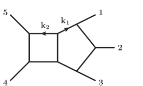
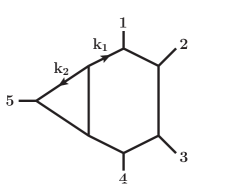
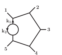
where the exponents, $a_{i}$, are integers and $d=4-2\epsilon$. The three master topologies, shown in Figure 1, are

Pentabox: $$G_{11111111a_{9}a_{10}a_{11}}$$ (7)

Hexatriangle: $$G_{111111a_{7}11a_{10}a_{11}}$$ (8)

Heptabubble: $$G_{21111a_{6}a_{7}11a_{10}a_{11}}$$ (9)

while propagators with unspecified exponents, $a_{j}$, correspond to ISPs (i.e. $a_{j}\leq 0$).

(a) Pentabox: $G_{11111111a_{9}a_{10}a_{11}}$

(b) Hexatriangle: $G_{111111a_{7}11a_{10}a_{11}}$

(c) Heptabubble: $G_{21111a_{6}a_{7}11a_{10}a_{11}}$

Figure 1: Two-loop five-point master topologies. All external momenta are considered out-going, arrows indicate loop momenta directions.

All lower point topologies are obtained by systematically pinching the propagators of the master topologies. Topologies with scaleless integrals are discarded since we work in dimensional regularisation. Pinching of propagators from different master topologies can lead to the same sub-topology. This happens in particular when all five cyclic permutations of the external momenta are included. In these cases the assignment to a master topology is not unique. The full set of 57 distinct topologies with a specific choice of master topology assignment is shown in Figure 2.

(a) Topologies associated with the pentabox master topology (top left), see (7).

(b) Topologies associated with the hexatriangle master topology (top left), see (8).

(c) Topologies associated with the heptabubble master topology (top left), see (9).

(d) Topologies with divergent cuts that must be computed simultaneously with sub-topologies of the heptabubble master topology in Figure 2(c).

Figure 2: All distinct two-loop five-point topologies.

We parametrise the integrand numerators by writing the most general polynomials in the ISPs subject to a power counting constraint from renormalizability considerations. As an example, the pentabox of Figure 1(a) has the numerator parametrisation,

$$\Delta\left(\parbox{48.36958pt}{ \includegraphics[width=56.9055pt]{figures/pentabox}}\right)=\sum c_{(1,1,1,1,1,1,1,1,a_{9},a_{10},a_{11})}(k_{1}+p_{5})^{-2a_{9}}(k_{2}+p_{1})^{-2a_{10}}(k_{2}+p_{1}+p_{2})^{-2a_{11}}$$ (10)

where the sum is truncated by the constraints on the exponents:

$$-5 \leq a_{9} \leq 0,$$ (11)

$$-4 \leq a_{10}+a_{11} \leq 0,$$ (12)

$$-7 \leq a_{9}+a_{10}+a_{10} \leq 0.$$ (13)

Each topology has $11-n$ ISPs where $n$ is the number of distinct propagators. The five cyclic permutations of the external legs give a total of 425 irreducible numerators.

Integrand representations of the form (10) are less compact than representations making use of, for example, local integrands, spurious integrands, and extra-dimensional ISPs ArkaniHamed:2010kv ; ArkaniHamed:2010gh ; Badger:2013gxa ; Badger:2015lda ; Badger:2016ozq ; Badger:2017jhb ; Bourjaily:2017wjl . However, in our set-up the integrand is only sampled numerically and not analytically reconstructed. Simplification at the integrand level is therefore not a priority. Because our final integrated amplitude does not depend on the choice of integrand parametrisation, we have chosen a form which is directly compatible with IBPs, rather than one yielding a compact integrand representation. On the other hand there is potential for considerable improvements in the efficiency of the algorithm if a simpler integrand form could be identified.

We take a top down approach to solving the complete system of integrands which, apart from the basis choice described above, is identical to the approach taken in Ref. Badger:2017jhb . The tree amplitudes used to compute the generalised unitarity cuts are evaluated by contracting Berends-Giele currents Berends:1987me as described in Peraro:2016wsq and the six-dimensional spinor-helicity formalism Cheung:2009dc . Eight topologies, shown in Figure 2(d), have divergent cuts and their integrand coefficients are determined simultaneously with sub-topologies in the heptabubble group, see Figure 2(c).

The numerical sampling of the integrand can show quickly which coefficients vanish and hence what integrals require further reduction using IBPs. The number of non-vanishing coefficients at the integrand level split into the components of $d_{s}=2,(d_{s}-2),(d_{s}-2)^{2}$ are $4387,14545,4420$ respectively. We find the maximum rank to be 5 for genuine two-loop topologies and rank 6 for a few integrals in the $(d_{s}-2)^{2}$ component of the amplitude that can be written as (1-loop)² integrals, see Figure 2(a).

At the end of the integrand reduction stage, the colour ordered amplitude can be written as

$$A^{(2)}\left(1,2,3,4,5\right)=\sum_{\mathbf{a}}c^{[\partial{\rm A}]}_{\mathbf{a}}\ G_{\mathbf{a}},$$ (14)

where we sum over the tuples $\mathbf{a}=(a_{1},a_{2},a_{3},a_{4},a_{5},a_{6},a_{7},a_{8},a_{9},a_{10},a_{11})$. The coefficients $c^{[\partial{\rm A}]}_{\mathbf{a}}$ are rational functions in the momentum twistor variables only.

3.2 Integration-by-parts identities

Each integral appearing in (14) is reduced to a set of master integrals $J_{k}$,

$$G_{\mathbf{a}}=\sum_{k}c^{[{\rm IBP}]}_{\mathbf{a}k}J_{k},$$ (15)

where the sum runs over 155 master integrals (remembering that we include the 5 cyclic permutations of the integral family $G$). The reduction is obtained by solving a traditional Laporta system of IBP equations Laporta:2001dd . The system is generated in Mathematica with the help of LiteRed Lee:2012cn , and solved over finite fields with a custom general-purpose linear solver for sparse systems of equations. The master integrals are chosen to be the uniform weight functions identified by Gehrmann, Henn and Lo Presti Gehrmann:2018yef . The $c^{[{\rm IBP}]}_{\mathbf{a}k}$ are rational functions in the momentum twistor variables and the dimensional regularisation parameter $\epsilon$.

3.3 Map to pentagon functions

Our next step is to expand the master integrals into a basis of pentagon functions defined by Gehrmann, Henn and Lo Presti. These functions can be written in terms of Goncharov Polylogarithms. We take the results of expanding the master integrals in $\epsilon$ from reference Gehrmann:2018yef ,

$$J_{k}=\sum_{x=0}^{4}\sum_{l}c^{[\rm f]}_{kl;x}\,\epsilon^{x}\,m_{l;x}(f)+\mathcal{O}(\epsilon^{5}),$$ (16)

where $m_{l;x}(f)$ are monomials in the pentagon functions.

The amplitude can thus be written as a combination of pentagon functions

$$A^{(2)}\left(1,2,3,4,5\right)=\sum_{l,x}c^{[{\rm A}]}_{l;x}m_{l;x}(f)+\mathcal{O}(\epsilon),$$ (17)

where the coefficients are defined through matrix multiplication, from the three reduction steps

$$c^{[{\rm A}]}_{l;x}=\sum_{\mathbf{a},k}\sum_{x=0}^{4}c^{[\partial{\rm A}]}_{\mathbf{a}}\,c^{[{\rm IBP}]}_{\mathbf{a}k}\,c^{[\rm f]}_{kl;x}\,\epsilon^{x}.$$ (18)

We recall that, in the previous equation, there is also an implicit dependence on $\epsilon$ coming from the $c^{[{\rm IBP}]}_{\mathbf{a}k}$, which were defined in (15) to be the full coefficients of the IBP reduction. Hence, the coefficients $c^{[{\rm A}]}_{l;x}$ are rational functions of $\epsilon$ which need to be expanded, as we will explain in the next subsection.

The final step of the algorithm is to perform the same decomposition for the universal IR poles in (4). For this we need the one-loop master integrals expanded up to weight four and written in the same alphabet as the two-loop integrals. These results were obtained directly from the differential equations in a canonical basis. We then write the poles analytically as

$$\left[-\frac{r_{\Gamma}}{\epsilon^{2}}\sum_{j=1}^{5}\left(\frac{\mu_{R}^{2}e^{\gamma_{E}}}{-s_{j,j+1}}\right)^{\epsilon}\right]A^{(1),[i]}\left(1^{-}_{g},2^{+}_{g},3^{+}_{g},4^{+}_{g},5^{+}_{g}\right)=\sum_{l,x}c^{[\rm IR]}_{l;x}m_{l;x}(f)+\mathcal{O}(\epsilon).$$ (19)

Our numerical algorithm can then compute the difference:

$$c^{[{\rm F}]}_{l;x}=c^{[{\rm A}]}_{l;x}-c^{[\rm IR]}_{l;x}$$ (20)

which we will expand in $\epsilon$ to find the finite remainder. At this point we have constructed a numerical algorithm which combines integrand reduction, IBP reduction and expansion of the master integrals into a basis of polylogarithms. This algorithm can be used to compute the finite remainder of the two-loop amplitude through evaluations of generalised unitarity cuts over finite fields.

3.4 Laurent expansion

In the previous subsections we described a numerical calculation over finite fields of the coefficients $c^{[{\rm F}]}_{l;x}$. They are used in order to write the finite remainder, $F^{(2),[i]},$ of the amplitude in terms of known pentagon functions. The coefficients, computed as described above, are rational functions of $\epsilon$. However, because the calculation uses the expansion in (16) for the master integrals in terms of pentagon functions, it is only valid up to $\mathcal{O}(\epsilon)$. Here we are interested in the finite part of the Laurent expansion in $\epsilon$.

As mentioned before, in order to obtain this Laurent expansion, we first perform a full reconstruction of the functions $c^{[{\rm F}]}_{l;x}$ in $\epsilon$, for numerical values over finite fields of the momentum twistor variables. The reconstructed function can thus be expanded in $\epsilon$ up to the desired order. This yields a decomposition of the form

$$c^{[{\rm F}]}_{l;x}=\sum_{y=-4}^{0}\,c^{[{\rm F}]}_{l;x,y}\epsilon^{y}+\mathcal{O}(\epsilon),$$ (21)

where we are interested in the finite parts $c^{[{\rm F}]}_{l;x,0}$, while $c^{[{\rm F}]}_{l;x,y}=0$ for $y<0$. The finite remainder is therefore

$$F^{(2),[1]}\left(1^{-}_{g},2^{+}_{g},3^{+}_{g},4^{+}_{g},5^{+}_{g}\right)=\sum_{l}\sum_{x=0}^{4}c^{[{\rm F}]}_{l;x,0}\,m_{l;x}(f)+\mathcal{O}(\epsilon),$$ (22)

with $c^{[{\rm F}]}_{l;x,0}$ defined by the Laurent expansion in (21).

The algorithm described above numerically computes the coefficients $c^{[{\rm F}]}_{l;x,0}$ of the finite remainder of the amplitude over finite fields, for any numerical value of the kinematic invariants represented by the momentum twistor variables. Full analytic formulas for the coefficients $c^{[{\rm F}]}_{l;x,0}$, as rational functions of the momentum twistor variables, are reconstructed from multiple numerical evaluations. For this purpose, we use a slightly improved version of the multivariate reconstruction techniques presented in reference Peraro:2016wsq .

In the next section we give a compact form of this result, obtained from the one in terms of momentum twistor variables, after converting it into spinor products and momentum invariants via some additional algebraic manipulations.

4 Results

We present a compact form of the amplitude by making use of the symmetry $(1,2,3,4,5)\rightarrow(1,5,4,3,2)$ and extracting an overall phase written in terms of spinor products,

$$F^{(L),[i]}\left(1^{-}_{g},2^{+}_{g},3^{+}_{g},4^{+}_{g},5^{+}_{g}\right)=\frac{[25]^{2}}{[12]\langle 23\rangle\langle 34\rangle\langle 45\rangle[51]}\left(F_{\rm sym}^{(L),[i]}(1,2,3,4,5)+F_{\rm sym}^{(L),[i]}(1,5,4,3,2)\right),$$ (23)

where $L$ labels the loop order and $i$ labels the component in the expansion around $d_{s}=2$. The known result at one-loop can be written as:

$$F_{\rm sym}^{(1),[1]}(1,2,3,4,5)=\frac{\operatorname{\rm tr}_{+}(2315)^{2}\operatorname{\rm tr}_{+}(1243)}{3s_{25}^{2}s_{23}s_{34}s_{15}}-\frac{\operatorname{\rm tr}_{+}(2543)}{6s_{34}},$$ (24)

where $\operatorname{\rm tr}_{+}(ijkl)=\frac{1}{2}\operatorname{\rm tr}((1+\gamma_{5})\not{p}_{i}\not{p}_{j}\not{p}_{k}\not{p}_{l})$ and $s_{ij}=(p_{i}+p_{j})^{2}$.

The finite parts of the two-loop amplitude can be written compactly in terms of weight two functions, just as at one-loop. We therefore follow the same strategy as at one-loop to find a basis of integral functions free of large cancellations due to spurious singularities. We find that a convenient basis for the $d_{s}-2$ component of the amplitude is

$$F_{\rm sym}^{(2),[1]}(1,2,3,4,5)= \quad c_{51}^{(2)}F^{(2)}_{\mathrm{box}}(s_{23},s_{34},s_{15})+c_{51}^{(1)}F^{(1)}_{\mathrm{box}}(s_{23},s_{34},s_{15})+c_{51}^{(0)}F^{(0)}_{\mathrm{box}}(s_{23},s_{34},s_{15})$$

$$+c_{34}^{(2)}F^{(2)}_{\mathrm{box}}(s_{12},s_{15},s_{34})+c_{34}^{(1)}F^{(1)}_{\mathrm{box}}(s_{12},s_{15},s_{34})+c_{34}^{(0)}F^{(0)}_{\mathrm{box}}(s_{12},s_{15},s_{34})$$

$$+c_{45}F^{(0)}_{\mathrm{box}}(s_{12},s_{23},s_{45})+c_{34;51}\hat{L}_{1}(s_{34},s_{15})+c_{51;23}\hat{L}_{1}(s_{15},s_{23})+c_{\rm rat},$$ (25)

and

$$F_{\rm sym}^{(2),[2]}(1,2,3,4,5)= \quad d_{34}^{(3)}F^{(3)}_{\mathrm{box}}(s_{12},s_{15},s_{34})+d_{34}^{(2)}F^{(2)}_{\mathrm{box}}(s_{12},s_{15},s_{34})$$

$$+d^{(3)}_{34;51}\hat{L}_{3}(s_{34},s_{15})+d^{(2)}_{34;51}\hat{L}_{2}(s_{34},s_{15})$$

$$+d^{(3)}_{51;23}\hat{L}_{3}(s_{15},s_{23})+d^{(2)}_{51;23}\hat{L}_{2}(s_{15},s_{23})+d_{\rm rat},$$ (26)

for the $(d_{s}-2)^{2}$ amplitude.

The integral functions are written in terms of simple logarithms and di-logarithms. All weight one functions appear as logarithms of ratios of kinematic invariants,

$$L_{k}(s,t)= \frac{\log(t/s)}{(s-t)^{k}},$$ (27)

where the singular behaviour is removed by defining,

$$\hat{L}_{0}(s,t)= L_{0}(s,t),$$ (28a)

$$\hat{L}_{1}(s,t)= L_{1}(s,t),$$ (28b)

$$\hat{L}_{2}(s,t)= L_{2}(s,t)+\frac{1}{2(s-t)}\left(\frac{1}{s}+\frac{1}{t}\right),$$ (28c)

$$\hat{L}_{3}(s,t)= L_{3}(s,t)+\frac{1}{2(s-t)^{2}}\left(\frac{1}{s}+\frac{1}{t}\right).$$ (28d)

At weight two all functions can be written in terms of the six-dimensional box function,

$$F^{(-1)}_{\mathrm{box}}(s,t,m^{2})= \mathrm{Li}_{2}\left(1-\frac{s}{m^{2}}\right)+\mathrm{Li}_{2}\left(1-\frac{t}{m^{2}}\right)+\log\left(\frac{s}{m^{2}}\right)+\log\left(\frac{t}{m^{2}}\right)-\frac{\pi^{2}}{6},$$ (29a)

$$F^{(0)}_{\mathrm{box}}(s,t,m^{2})= \frac{1}{u(s,t,m^{2})}F^{(-1)}_{\mathrm{box}}(s,t,m^{2}),$$ (29b)

$$F^{(1)}_{\mathrm{box}}(s,t,m^{2})= \frac{1}{u(s,t,m^{2})}\left[F^{(0)}_{\mathrm{box}}(s,t,m^{2})+\hat{L}_{1}(s,m^{2})+\hat{L}_{1}(m^{2},t)\right],$$ (29c)

$$F^{(2)}_{\mathrm{box}}(s,t,m^{2})= \frac{1}{u(s,t,m^{2})}\Bigg{[}F^{(1)}_{\mathrm{box}}(s,t,m^{2})+\frac{s-m^{2}}{2t}\hat{L}_{2}(s,m^{2})+\frac{m^{2}-t}{2s}\hat{L}_{2}(m^{2},t)$$

$$-\left(\frac{1}{s}+\frac{1}{t}\right)\frac{1}{4m^{2}}\big{]},$$ (29d)

$$F^{(3)}_{\mathrm{box}}(s,t,m^{2})= \frac{1}{u(s,t,m^{2})}\big{[}F^{(2)}_{\mathrm{box}}(s,t,m^{2})-\frac{(s-m^{2})^{2}}{6t^{2}}\hat{L}_{3}(s,m^{2})-\frac{(m^{2}-t)^{2}}{6s^{2}}\hat{L}_{3}(m^{2},t)$$

$$-\left(\frac{1}{s}+\frac{1}{t}\right)\frac{1}{6m^{4}}\Bigg{]},$$ (29e)

where $u(s,t,m^{2})=m^{2}-s-t$.

These functions serve the same purpose as the $Ls$ and $L$ functions introduced by Bern, Dixon, and Kosower in Bern:1993mq ; Bern:1994fz . The $\hat{L}_{i}(s,t)$ are finite as $s\to t$ and the $F^{(i)}_{\mathrm{box}}(s,t,m^{2})$ are finite as $s\to-t+m^{2}$. The definitions have been changed very slightly with respect to the $Ls$ and $L$ functions since the singularities from the box functions at $m^{2}-s-t$ have been removed without introducing additional singularities in $s-m^{2}$ or $t-m^{2}$.

For the $(d_{s}-2)$ amplitude the coefficients are:

$$c_{51}^{(2)}= \frac{5s_{23}s_{34}\operatorname{\rm tr}_{+}(1234)^{2}\operatorname{\rm tr}_{+}(1542)^{2}}{s_{12}s_{15}\operatorname{\rm tr}_{+}(2543)^{2}},$$ (30a)

$$c_{51}^{(1)}= -\frac{\operatorname{\rm tr}_{+}(1234)^{2}\operatorname{\rm tr}_{+}(1534)\operatorname{\rm tr}_{+}(2453)^{2}}{6s_{12}s_{34}s_{35}\operatorname{\rm tr}_{+}(2543)^{2}},$$ (30b)

$$c_{51}^{(0)}= \frac{s_{15}s_{45}\operatorname{\rm tr}_{+}(1234)}{3\operatorname{\rm tr}_{+}(2543)}-\frac{s_{15}s_{24}s_{45}\operatorname{\rm tr}_{+}(1234)^{2}}{6s_{12}\operatorname{\rm tr}_{+}(2543)^{2}}-\frac{\operatorname{\rm tr}_{+}(1234)^{2}\operatorname{\rm tr}_{+}(1542)}{6\operatorname{\rm tr}_{+}(2543)^{2}}$$

$$-\frac{s_{23}s_{24}\operatorname{\rm tr}_{+}(1234)\operatorname{\rm tr}_{+}(1543)}{6\operatorname{\rm tr}_{+}(2543)^{2}}-\frac{s_{12}s_{23}s_{34}\operatorname{\rm tr}_{+}(1542)\operatorname{\rm tr}_{+}(1543)}{3s_{15}\operatorname{\rm tr}_{+}(2543)^{2}}$$

$$+\frac{2s_{23}\operatorname{\rm tr}_{+}(1234)\operatorname{\rm tr}_{+}(1543)^{2}}{3s_{15}\operatorname{\rm tr}_{+}(2543)^{2}}-\frac{s_{24}\operatorname{\rm tr}_{+}(1234)\operatorname{\rm tr}_{+}(1543)^{2}}{6s_{15}\operatorname{\rm tr}_{+}(2543)^{2}}$$

$$-\frac{s_{24}\operatorname{\rm tr}_{+}(1234)^{2}\operatorname{\rm tr}_{+}(1543)^{2}}{6s_{12}s_{15}s_{34}\operatorname{\rm tr}_{+}(2543)^{2}}-\frac{s_{24}\operatorname{\rm tr}_{+}(1235)\operatorname{\rm tr}_{+}(1243)\operatorname{\rm tr}_{+}(1543)^{2}}{6s_{12}s_{15}s_{34}\operatorname{\rm tr}_{+}(2543)^{2}}$$

$$-\frac{\operatorname{\rm tr}_{+}(1234)\operatorname{\rm tr}_{+}(1543)\operatorname{\rm tr}_{+}(2453)}{2\operatorname{\rm tr}_{+}(2543)^{2}},$$ (30c)

$$c_{34}^{(2)}= \frac{5}{2}s_{12}^{2}s_{15}^{2},$$ (31a)

$$c_{34}^{(1)}= \frac{\operatorname{\rm tr}_{+}(1245)\operatorname{\rm tr}_{+}(1534)\operatorname{\rm tr}_{+}(1543)}{3s_{15}s_{34}s_{45}}+\frac{1}{12}s_{12}s_{15}s_{34},$$ (31b)

$$c_{34}^{(0)}= -\frac{s_{15}s_{23}\operatorname{\rm tr}_{+}(1234)}{12\operatorname{\rm tr}_{+}(2543)}-\frac{\operatorname{\rm tr}_{+}(1234)^{2}\operatorname{\rm tr}_{+}(1532)}{12s_{12}s_{34}\operatorname{\rm tr}_{+}(2543)}+\frac{s_{25}\operatorname{\rm tr}_{+}(1234)\operatorname{\rm tr}_{+}(1543)}{12s_{34}\operatorname{\rm tr}_{+}(2543)}$$

$$+\frac{s_{12}\operatorname{\rm tr}_{+}(1532)\operatorname{\rm tr}_{+}(1543)}{12s_{15}\operatorname{\rm tr}_{+}(2543)}+\frac{s_{23}s_{25}\operatorname{\rm tr}_{+}(1234)\operatorname{\rm tr}_{+}(1543)^{2}}{12s_{15}s_{34}\operatorname{\rm tr}_{+}(2543)^{2}}$$

$$+\frac{s_{12}\operatorname{\rm tr}_{+}(1543)^{2}\operatorname{\rm tr}_{+}(2354)}{12s_{15}s_{34}s_{45}\operatorname{\rm tr}_{+}(2543)}+\frac{s_{25}\operatorname{\rm tr}_{+}(2543)}{12s_{34}}-\frac{1}{3}s_{12}s_{15},$$ (31c)

$$c_{45}=-\frac{s_{13}s_{45}\operatorname{\rm tr}_{+}(1234)^{2}\operatorname{\rm tr}_{+}(1534)}{6s_{12}s_{34}\operatorname{\rm tr}_{+}(2543)^{2}}+\frac{s_{23}^{3}s_{34}\operatorname{\rm tr}_{+}(1543)}{6\operatorname{\rm tr}_{+}(2543)^{2}}-\frac{s_{13}s_{23}\operatorname{\rm tr}_{+}(1243)\operatorname{\rm tr}_{+}(1543)^{2}}{6s_{15}s_{34}\operatorname{\rm tr}_{+}(2543)^{2}},$$ (32)

$$c_{34;51}=\ \frac{s_{12}s_{15}s_{34}s_{45}}{6\operatorname{\rm tr}_{+}(2543)}-\frac{11\operatorname{\rm tr}_{+}(1234)\operatorname{\rm tr}_{+}(1543)}{6\operatorname{\rm tr}_{+}(2543)}+\frac{\operatorname{\rm tr}_{+}(1234)^{2}\operatorname{\rm tr}_{+}(1542)\operatorname{\rm tr}_{+}(1543)}{6s_{12}s_{34}\operatorname{\rm tr}_{+}(2543)^{2}}$$

$$-\frac{s_{12}\operatorname{\rm tr}_{+}(1324)\operatorname{\rm tr}_{+}(1543)^{2}}{6s_{13}\operatorname{\rm tr}_{+}(2543)^{2}}-\frac{s_{45}\operatorname{\rm tr}_{+}(1234)^{2}\operatorname{\rm tr}_{+}(1534)\operatorname{\rm tr}_{+}(2453)}{6s_{12}s_{34}s_{35}\operatorname{\rm tr}_{+}(2543)^{2}},$$ (33)

$$c_{51;23}=\ \frac{s_{23}s_{45}\operatorname{\rm tr}_{+}(1234)^{2}\operatorname{\rm tr}_{+}(1534)}{6s_{12}s_{34}\operatorname{\rm tr}_{+}(2543)^{2}}+\frac{2s_{12}s_{23}s_{34}s_{45}\operatorname{\rm tr}_{+}(1543)}{3\operatorname{\rm tr}_{+}(2543)^{2}}$$

$$-\frac{5s_{23}s_{45}\operatorname{\rm tr}_{+}(1234)\operatorname{\rm tr}_{+}(1543)}{2\operatorname{\rm tr}_{+}(2543)^{2}},$$ (34)

$$c_{\rm rat}=\ -\frac{5\operatorname{\rm tr}_{+}(1234)\operatorname{\rm tr}_{+}(1543)}{4s_{34}\operatorname{\rm tr}_{+}(2543)}+\frac{5s_{23}\operatorname{\rm tr}_{+}(1243)\operatorname{\rm tr}_{+}(1543)^{2}}{2s_{15}s_{34}\operatorname{\rm tr}_{+}(2543)^{2}}.$$ (35)

While for the $(d_{s}-2)^{2}$ amplitude the coefficients are:

$$d_{34}^{(3)}= -\frac{s_{12}s_{15}\operatorname{\rm tr}_{+}(2543)^{2}}{12s_{34}},$$ (36a)

$$d_{34}^{(2)}= \frac{1}{6}s_{12}s_{15}\operatorname{\rm tr}_{+}(2543),$$ (36b)

$$d_{34;51}^{(3)}= -\frac{1}{18}s_{15}s_{23}\operatorname{\rm tr}_{+}(2543),$$ (36c)

$$d_{34;51}^{(2)}= -\frac{s_{15}\operatorname{\rm tr}_{+}(2543)^{2}}{36s_{12}s_{34}}-\frac{1}{6}s_{15}\operatorname{\rm tr}_{+}(2543),$$ (36d)

$$d_{51;23}^{(3)}= \frac{s_{15}s_{23}s_{34}^{2}s_{45}^{2}\operatorname{\rm tr}_{+}(1245)}{18\operatorname{\rm tr}_{+}(2543)^{2}},$$ (37a)

$$d_{51;23}^{(2)}= \frac{s_{12}s_{15}s_{23}s_{34}^{2}s_{45}^{2}}{12\operatorname{\rm tr}_{+}(2543)^{2}}-\frac{s_{15}s_{23}s_{34}s_{45}^{2}\operatorname{\rm tr}_{+}(1234)}{6\operatorname{\rm tr}_{+}(2543)^{2}},$$ (37b)

$$d_{\rm rat}= \frac{s_{34}}{72}+\frac{5s_{45}}{36}-\frac{\operatorname{\rm tr}_{+}(1234)\operatorname{\rm tr}_{+}(1453)}{72s_{14}\operatorname{\rm tr}_{+}(2543)}-\frac{s_{45}\operatorname{\rm tr}_{+}(1543)}{72\operatorname{\rm tr}_{+}(2543)}+\frac{\operatorname{\rm tr}_{+}(2543)^{2}}{72s_{34}^{3}}$$

$$-\frac{5\operatorname{\rm tr}_{+}(1543)^{2}}{72s_{34}\operatorname{\rm tr}_{+}(2543)}-\frac{s_{12}\operatorname{\rm tr}_{+}(1543)^{2}}{72\operatorname{\rm tr}_{+}(2543)^{2}}+\frac{s_{23}s_{34}s_{45}\operatorname{\rm tr}_{+}(1543)}{18\operatorname{\rm tr}_{+}(2543)^{2}}.$$ (38)

These results can also be found in the ancillary file included with the arXiv version of this article.

5 Conclusions

In this article we have presented a new analytic result for a two-loop five-gluon scattering amplitude in QCD. We were able to find a compact representation for the finite remainder of the single-minus helicity configuration after removing the universal infrared poles. We set up a complete tool-chain from generalised unitarity cuts to the coefficients of a basis of pentagon functions for the finite remainder. This numerical algorithm was then evaluated multiple times with finite field arithmetic and the analytic result reconstructed, avoiding the usual large intermediate expressions.

This single-minus amplitude has turned out to be significantly more difficult to compute than the highly symmetric all-plus helicity amplitude that has been known for some time Badger:2013gxa ; Gehrmann:2015bfy . At the level of the master integrals the single-minus amplitude was of similar complexity to the maximal-helicity-violating (MHV) configurations. However, after removing the contribution from the universal poles, the finite remainder was simple and contained only up to weight two polylogarithms. This makes the final answer simpler than the more general MHV case which will have up to weight four polylogarithms.

Nevertheless, the techniques presented here are not helicity dependent so we hope to find applications to the remaining independent planar helicity amplitudes in the near future. The last few months have also seen progress on non-planar integrals Chicherin:2017dob ; Abreu:2018rcw ; Chicherin:2018mue for five-point scattering which is encouraging for applications to non-planar amplitudes.