Stably stratified stars containing magnetic fields whose toroidal components are much larger than the poloidal ones in general relativity – A perturbation analysis –

Abstract

We construct the stably stratified magnetized stars within the framework of general relativity. The effects of magnetic fields on the structure of the star and spacetime are treated as perturbations of non-magnetized stars. By assuming ideal magnetohydrodynamics and employing one-parameter equations of state, we derive basic equations for describing stationary and axisymmetric stably stratified stars containing magnetic fields whose toroidal components are much larger than the poloidal ones. A number of the polytropic models are numerically calculated to investigate basic properties of the effects of magnetic fields on the stellar structure. According to the stability result obtained by Braithwaite, which remains a matter of conjecture for general magnetized stars, certain of the magnetized stars constructed in this study are possibly stable.

I Introduction

It has been well-accepted that soft-gamma repeaters (SGRs) and anomalous x-ray pulsars (AXPs) are magnetars, highly magnetized neutron stars whose strength of the surface field is as large as $\sim 10^{14}-10^{15}$ G duncan ; paczynsk ; thompsona ; thompsonb ; woods . The existence of the magnetar has reactivated studies on equilibrium configurations of magnetized stars.

In order to elucidate basic properties of equilibrium configurations of magnetized stars, a large number of studies have been performed so far since the pioneering work of Chandrasekhar and Fermi chandra . A large fraction of those studies have been done within the framework of Newtonian magnetohydrodynamics and Newton’s theory of gravity (cf., e.g., Refs. prendergast ; woltjer ; roxburgh ; trehanb ; monaghana ; monaghanb ; sinha ; trehana ; ioka ; miketinac ; miketinac2 ; tomimura ; yoshida0 ; yoshida ; lander ; fujisawaa ; fujisawab ; duez ). Since neutron stars are very compact in the sense that their compactness $M/R$ is as large as $\sim 0.1-0.2$ with $M$ and $R$ being their mass and radius in geometrical units, general relativity is required to describe the gravitational field of neutron stars. Therefore, general relativistic models of magnetized stars have been investigated as well. Bocquet et al. bocquet and Cardall et al. cardall obtained relativistic neutron star models with purely poloidal magnetic fields. Using a perturbative technique, Konno et al. konno calculated similar models to those obtained in Refs. bocquet ; cardall . Kiuchi and Yoshida kiuchi computed magnetized stars with purely toroidal fields (cf., also, Ref. frieben ). Ioka and Sasaki Ioka2004 , Colaiuda et al. colaiuda , and Ciolfi et al. ciolfia ; ciolfib derived relativistic stellar models having both toroidal and poloidal magnetic fields with perturbative techniques (cf., also, Ref. ciolfic ). Yoshida et al. yoshidaa included the effects of the stable stratification in the magnetized star model obtained in Ref. Ioka2004 . Uryu et al. uryua ; uryub obtained magnetized stars with mixed poloidal-toroidal magnetic fields by solving a full set of Einstein equations, magnetohydrodynamics equations, and coordinate conditions numerically. By assuming simpler conformally flat spacetime, Pili et al. pilia ; pilib ; bucciantini ; pilic calculated many models of magnetized stars. Although great progress has been achieved in this field, as mentioned before, further studies are required because all the magnetized star models are constructed by some particular magnetic-field configurations which are not necessarily realistic. In particular, it is not still clear at all whether stable models exist.

Stability of magnetized stars with a relatively simple magnetic field structure have been examined with analytical approaches. The pioneering work was done by Tayler tayler73 , who showed that stars with purely toroidal magnetic fields are unstable. Wright wright73 subsequently showed that the same instability mechanism, the pinch-type instability mechanism, operates in stars with purely poloidal magnetic fields. He also suggested the possibility that stars having mixed poloidal-toroidal magnetic fields may be stable if the strength of both components is comparable (cf., also, Refs. markey ; tayler80 ; assche ). Flowers and Ruderman flowers found that another type of instability occurs in purely poloidal magnetic field configurations. All those classical stability analyses were based on a method of an energy principle in the framework of Newtonian dynamics (cf., also, Refs. pitts ; goossens ). Another approach is a local analysis, with which Acheson acheson1978 investigated the stability of rotating magnetized stars containing purely toroidal fields in detail within the framework of Newtonian dynamics (cf., also, Refs. acheson1979 ; spruit ) and derived detailed stability conditions for purely toroidal magnetic fields buried inside rotating stars with dissipation. Bonanno and Urpin analyzed the axisymmetric stability bonanno and the non-axisymmetric stability bonanno2 of cylindrical equilibrium configurations possessing mixed poloidal-toroidal fields, while ignoring compressibility and stratification of the fluid.

Recently the stability problem of the magnetized star has been approached from another direction, dynamical simulation approaches, and some significant progress has been made. By following the time evolution of small random initial magnetic fields around a spherical star in the framework of Newtonian resistive magnetohydrodynamics, Braithwaite and Spruit Braithwaite2004 ; Braithwaite2006 obtained stable equilibria of magnetized stars that are formed as a self-organization phenomenon. The resulting stable magnetic fields have both poloidal and toroidal components with comparable strength and support the conjecture for stability conditions of the magnetized star given by the classical studies mentioned before (cf., also, Ref. duez10 ). By using the numerical magnetohydrodynamic simulation, Braithwaite Braithwaite2009 studied stability conditions for the magnetized stars and obtained a stability condition for his models given in terms of the ratio of the poloidal magnetic energy to the total magnetic energy. The stability condition is given by

$$\tilde{a}{E_{\rm EM}\over|W|}<{E_{\rm EM}^{(p)}\over E_{\rm EM}}\lesssim 0.8\,,$$ (1)

where $E_{\rm EM}$, $E_{\rm EM}^{(p)}$, and $W$ are the total magnetic energy, the poloidal magnetic energy, and the gravitational energy, respectively, and $\tilde{a}$ is a dimensionless factor related to the buoyancy properties of the star. For neutron stars and main-sequence stars, the dimensionless factor $\tilde{a}$ is of order $10^{3}$ and $10$, respectively. Lander and Jones examined the stability of magnetized stars by numerically solving the time evolution of linear perturbations of the stars in their series of papers lander11 ; lander11b ; lander12 . For the stars with purely toroidal and purely poloidal magnetic fields, their results are consistent with those of the classical stability analysis, i.e., the pinch-type instability occurs near the symmetry and the magnetic axes for the cases of the purely toroidal and the purely poloidal magnetic fields, respectively (cf., also, Refs. kiuchia ; kiuchib ; ciolfid ; lasky ; ciolfie ; zink ). They also assessed the stability of various magnetized stars with mixed poloidal-toroidal fields and found that all their models considered suffer from the pinch-type instability even for the cases in which the poloidal and toroidal components have comparable strength lander12 . At first glance, it seems that the results by Lander and Jones are incompatible with those by Braithwaite and his collaborators Braithwaite2009 ; duez10 . Mitchell et al. mitchell made numerical simulations smilar to those of Braithwaite and his collaborators Braithwaite2004 ; Braithwaite2006 but for the case of the non-stratified star. They then obtained no stable equilibrium for the non-stratified case and showed that stable stratification of the fluid will be a key ingredient, which is taken into account in the analyses of Refs. Braithwaite2009 ; duez10 but not in the analyses of Ref. lander12 . In other words, the results obtained by Mitchell et al. mitchell suggest that stable stratification is required to avoid instability for some magnetic-field configurations inside the star. Note that in the simulations by Braithwaite and his collaborators Braithwaite2004 ; Braithwaite2006 , resistive dissipation will also play a crucial role. Therefore, effects of the resistive dissipation on dynamical stability of the magnetized star need to be closely examined.

Despite the fact that a large number of studies on equilibria and stabilities of magnetized stars have been made so far, as mentioned before, the magnetic field structure of the neutron star has not yet been elucidated not only theoretically but also observationally. The formation process of the neutron star would however provide us with some clues. During the core collapse events which produce neutron stars, the poloidal magnetic field lines would get wrapped around the rotation axis because of the differential rotation of the core (cf., e.g., Ref. kotake ). As a result, the toroidal field would be significantly amplified. It is therefore likely to expect that the toroidal component of the magnetic field is much larger than the poloidal one inside the neutron star at least soon after its birth.

To investigate properties of the magnetized star whose toroidal fields are much larger than the poloidal ones, Kiuchi and Yoshida kiuchi constructed the magnetized stars completely neglecting the poloidal component of the magnetic field. Although studies on stars with purely toroidal magnetic fields can elucidate approximate properties of magnetized stars whose toroidal fields are much larger than the poloidal ones, purely toroidal magnetic fields inside the star are unstable as mentioned before. To stabilize the toroidal magnetic field inside the star, the inclusion of the poloidal magnetic field is necessary. To our knowledge, however, equilibrium states of the magnetized star whose toroidal fields are much larger than the poloidal ones, which are plausible neutron star models, have not been constructed so far, except the case of purely toroidal magnetic fields. As mentioned before, another important stabilizing agent for magnetic fields inside the star is a stable stratification of the fluid. In order to construct neutron star models with more realistic interior magnetic field structure, in this study, we investigate stably stratified stars having magnetic fields characterized by the condition of ${E_{\rm EM}^{(p)}/E_{\rm EM}}\ll 1$, i.e., the toroidal field is much larger than the poloidal one, within the framework of general relativity.

The strength of the effects of magnetic fields on the stellar structure can be roughly estimated by an approximate ratio of the magnetic field energy, $E_{\rm EM}$, to the gravitational energy, $W$, given by

$${E_{\rm EM}\over|W|}\approx 10^{-6}\left({B_{0}\over 10^{15}\,{\rm G}}\right)^{2}\left({R\over 10\,{\rm km}}\right)^{4}\left({M\over 1.4\,M_{\odot}}\right)^{-2}\,,$$ (2)

where $B_{0}$, $R$, and $M$ are the strength of the magnetic field, the radius, and the mass of the star, respectively. This ratio is very small even if a magnetar characterized by $B_{0}\sim 10^{15}\,{\rm G}$ is considered. In order to investigate effects of magnetic fields on the neutron star structure, therefore, perturbation approaches are generally quite efficient in the sense that they are tractable and give sufficiently accurate results. We therefore make use of a perturbation approach to study the structure of the magnetized star in this work.

The present paper is organized as follows. In Section II, we introduce the general formalism for general relativistic ideal magnetohydrodynamics. Section III presents the formalism used to construct the stably stratified magnetized star whose toroidal fields are much larger than the poloidal ones. In Section IV, we exhibit examples of the stably stratified magnetized stars calculated numerically. Finally, we give the discussion and summary in Sections V and VI, respectively. In Appendix, we give a Newtonian analysis of the same magnetized star as that discussed in this paper. In the following, we choose the signature $(-,+,+,+)$ for the spacetime metric and, unless otherwise stated, we adopt geometrical units with $c=G=1$, where $c$ and $G$ are the speed of light and Newton’s gravitational constant, respectively.

II Basic equations describing dynamics of perfectly conductive fluids

The dynamics of perfect fluids coupled with electromagnetic fields may be described by the magnetohydrodynamics equations summarized as follows. Baryon mass conservation equation:

$$\nabla_{\mu}\left(\rho u^{\mu}\right)=0\,,$$ (3)

where $\rho$ and $u^{\mu}$ are the rest-mass density and the fluid four-velocity, respectively. Here, $\nabla_{\mu}$ denotes the covariant derivative associated with the metric $g_{\mu\nu}$, and spacetime indices are denoted by lower case Greek letters ($\alpha,\beta,\gamma,\cdots$). The Maxwell equations:

$$\nabla_{\alpha}F_{\mu\nu}+\nabla_{\mu}F_{\nu\alpha}+\nabla_{\nu}F_{\alpha\mu}=0\,,$$ (4)

$$\nabla_{\nu}F^{\mu\nu}=4\pi J^{\mu}\,,$$ (5)

where $F_{\mu\nu}$ and $J^{\mu}$ are the Faraday tensor and the current four-vector, respectively. The conservation law of the energy-momentum tensor:

$$\nabla_{\nu}T^{\mu\nu}=0\,,$$ (6)

where $T^{\mu\nu}$ is the energy-momentum tensor, defined by

$$T^{\mu\nu} = \rho hu^{\mu}u^{\nu}+Pg^{\mu\nu}$$ (7)

$$+{1\over 4\pi}\left[F^{\mu\alpha}{F^{\nu}}_{\alpha}-{1\over 4}g^{\mu\nu}F^{\alpha\beta}F_{\alpha\beta}\right]\,,$$

where $h$ and $P$ are the specific enthalpy and the pressure, respectively. Here, the specific enthalpy may, in terms of the specific internal energy $\varepsilon$, the pressure $P$, and the rest-mass density $\rho$, be defined by

$$h=1+\varepsilon+{P\over\rho}\,.$$ (8)

As for the equations of state, we supply one-parameter equations of state, given by

$$P=P\left(\rho\right)\,,\quad\varepsilon=\varepsilon\left(\rho\right)\,.$$ (9)

The electric field $E_{\mu}$ and the magnetic field $B_{\mu}$ observed by an observer associated with the fluid four-velocity $u^{\mu}$ are defined by

$$E_{\mu} = F_{\mu\nu}u^{\nu}\,,$$ (10)

$$B_{\mu} = {1\over 2}\epsilon_{\nu\mu\alpha\beta}u^{\nu}F^{\alpha\beta}\,,$$ (11)

where $\epsilon_{\mu\nu\alpha\beta}$ is the Levi-Civita tensor with $\epsilon_{0123}=\sqrt{-g}$. Here, $g$ denotes the determinant of the metric $g_{\mu\nu}$. Since the neutron-star matter may be approximately assumed as a perfect conductor, in this study, we may further impose the condition of perfect conductivity, given by

$$E_{\mu}=F_{\mu\nu}u^{\nu}=0\,.$$ (12)

Equation (6) may be divided into two equations, the energy equation and the momentum equations, respectively, given by

$$-u_{\mu}\nabla_{\nu}T^{\mu\nu} = u^{\mu}\nabla_{\nu}\left\{\rho\left(1+\varepsilon\right)\right\}+\rho h\nabla_{\nu}u^{\nu}$$ (13)

$$= \rho u^{\nu}\nabla_{\nu}\varepsilon+P\nabla_{\nu}u^{\nu}=0\,,$$

$$q_{\mu\alpha}\nabla_{\nu}T^{\alpha\nu} = \rho hu^{\nu}\nabla_{\nu}u_{\mu}+q_{\mu}^{\nu}\nabla_{\nu}P-F_{\mu\nu}J^{\nu}$$ (14)

$$= 0\,,$$

where $q_{\mu\nu}=g_{\mu\nu}+u_{\mu}u_{\nu}$. Note that the perfect conductivity condition (12) has been used in the derivation of Equation (13).

III Master equations for equilibrium solutions of the magnetized star

In order to obtain equilibrium solutions of the relativistic stars containing the mixed poloidal-toroidal magnetic fields, in this study, we make the following assumptions: (i) Equilibrium models are stationary and axisymmetric, i.e., the spacetime has the time Killing vector $t^{\mu}$ and the rotational Killing vector $\varphi^{\mu}$, and Lie derivatives of the equilibrium quantities along the Killing vectors $t^{\mu}$ and $\varphi^{\mu}$ vanish. (ii) There is no fluid flow. (iii) The magnetic fields are sufficiently weak in the sense that the magnetic effects on the equilibrium structures may be treated as perturbations of stars including no electromagnetic field. (iv) The toroidal component of magnetic fields is much larger than the poloidal one. Under these assumptions, we may derive the master equations for describing equilibrium states of the relativistic stars containing the mixed poloidal-toroidal magnetic fields using the magnetohydrodynamic equations summarized in the previous section.

In order to give a clear and definite description of the assumptions (iii) and (iv), we introduce two dimensionless smallness parameters $\varepsilon_{t}$ and $\varepsilon_{p}$ representing the amplitudes of the toroidal and the poloidal components of magnetic fields, respectively. We may then write that ${}^{(t)}F_{\mu\nu}{}^{(t)}F^{\mu\nu}\,P^{-1}=O\left(\varepsilon_{t}^{2}\right)$ and ${}^{(p)}F_{\mu\nu}{}^{(p)}F^{\mu\nu}\,P^{-1}=O\left(\varepsilon_{p}^{2}\right)$ where ${}^{(t)}F_{\mu\nu}$ and ${}^{(p)}F_{\mu\nu}$ stand for the toroidal and poloidal components of the Faraday tensor $F_{\mu\nu}$, respectively. Note that $F_{\mu\nu}$ can be divided into the two parts, ${}^{(t)}F_{\mu\nu}$ and ${}^{(p)}F_{\mu\nu}$, because of the assumptions of the stationary and axially symmetric magnetic fields and the perfectly conducting fluid without flow. By the assumption (iii) we have $\varepsilon_{t}\ll 1$ and $\varepsilon_{p}\ll 1$. By the assumption (iv) we further impose that $\varepsilon_{p}\ll\varepsilon_{t}\ll 1$.

In this study, as mentioned before, the unperturbed state is assumed to be a static and spherically symmetric star without magnetic fields. Around the spherically symmetric star, we may impose as perturbations the magnetic fields, given by

$$F_{\mu\nu}=\varepsilon_{t}{}^{(t)}F_{\mu\nu}+\varepsilon_{p}{}^{(p)}F_{\mu\nu}\,.$$ (15)

By this magnetic field, the matter distribution deviates from spherical symmetry. In this study, we are primarily interested in the lowest-order effects of the poloidal magnetic field on the structure of the star including purely toroidal magnetic fields. We therefore consider perturbations of order $\varepsilon_{t}^{2}$ and $\varepsilon_{t}\varepsilon_{p}$ on the structure of the spherically symmetric star but neglect perturbations of order higher than $\varepsilon_{p}^{2}$. Note that because of the assumption (iv), i.e., $\varepsilon_{p}\ll\varepsilon_{t}\ll 1$, we have the inequality $\varepsilon_{t}^{0}\varepsilon_{p}^{0}\gg\varepsilon_{t}^{2}\varepsilon_{p}^{0}\gg\varepsilon_{t}^{1}\varepsilon_{p}^{1}\gg\varepsilon_{t}^{0}\varepsilon_{p}^{2}\,.$

III.1 Static and spherically symmetric stars without magnetic fields: the $\varepsilon_{t}^{0}\varepsilon_{p}^{0}$-order equations

The line element of static and spherically symmetric spacetime may be given by

$$ds^{2} = {}^{(0)}g_{\mu\nu}dx^{\mu}dx^{\nu}$$ (17)

$$= -e^{2\nu}dt^{2}+e^{2\lambda}dr^{2}$$

$$\quad\quad+r^{2}\left(d\theta^{2}+\sin^{2}\theta\,d\varphi^{2}\right)\,,$$

where ${}^{(0)}g_{\mu\nu}$ denotes the unperturbed metric, and $\nu$ and $\lambda$ are functions of $r$ only. The equilibrium state of the unperturbed star is described by the following equations (cf., e.g., Ref. mtw ):

$${dM_{r}\over dr}=4\pi r^{2}{\,}^{(0)}\rho\left(1+{\,}^{(0)}\varepsilon\right)\,,$$ (18)

$${d{\,}^{(0)}P\over dr}=-e^{2\lambda}{\,}^{(0)}\rho{\,}^{(0)}h{M_{r}+4\pi{\,}^{(0)}Pr^{3}\over r^{2}}\,,$$ (19)

$${d\nu\over dr}=-{1\over{\,}^{(0)}\rho{\,}^{(0)}h}{d{\,}^{(0)}P\over dr}\,,$$ (20)

where $M_{r}$ is defined in terms of the metric function by

$$M_{r}={r\over 2}\left(1-e^{-2\lambda}\right)\,,$$ (21)

and ${\,}^{(0)}\rho$, ${\,}^{(0)}\varepsilon$, ${\,}^{(0)}P$, and ${\,}^{(0)}h$ are, respectively, the rest-mass density, specific internal energy, pressure, and specific enthalpy for the unperturbed star.

III.2 Magnetic fields around a spherical star: the $\varepsilon_{t}^{1}\varepsilon_{p}^{0}$ and $\varepsilon_{t}^{0}\varepsilon_{p}^{1}$ order equations

Due to the assumption of no fluid flow, the assumption (ii), the fluid four-velocity is given by

$$u^{\mu}=\gamma\,t^{\mu}\,,$$ (22)

where $\gamma$ is the function determined by the normalization condition $u^{\mu}u_{\mu}=-1$. The perfect-conductivity condition (12) then becomes

$$F_{\mu\nu}t^{\nu}=F_{\mu t}=0\,.$$ (23)

As argued by Kiuchi and Yoshida kiuchi , the toroidal component of the magnetic field may be characterized by the conditions, given by

$${}^{(t)}F_{\mu\nu}\varphi^{\nu}=0\,.$$ (24)

Thus, we see that the non-zero component of the toroidal magnetic field ${}^{(t)}F_{\mu\nu}$ is ${}^{(t)}F_{r\theta}\left(=-^{(t)}F_{\theta r}\right)$ only. The poloidal component of the magnetic field may be given in term of the poloidal flux function $\Psi$, which is actually the $\varphi$ component of the vector potential $A_{\mu}$, i.e., $\Psi=A_{\varphi}$ (cf., e.g., Ref. bocquet ). Under the present assumptions, therefore, the Faraday tensor may be given by

$$F_{\mu\nu} = \varepsilon_{t}{}^{(t)}F_{\mu\nu}+\varepsilon_{p}{}^{(p)}F_{\mu\nu}$$ (34)

$$= \varepsilon_{t}\,^{(t)}F_{r\theta}\left(\begin{array}[]{cccc}0&0&0&0\\ 0&0&1&0\\ 0&-1&0&0\\ 0&0&0&0\end{array}\right)$$

$$+\varepsilon_{p}\left(\begin{array}[]{cccc}0&0&0&0\\ 0&0&0&\partial_{r}\Psi\\ 0&0&0&\partial_{\theta}\Psi\\ 0&-\partial_{r}\Psi&-\partial_{\theta}\Psi&0\end{array}\right)\,,$$

where ${}^{(t)}F_{r\theta}$ and $\Psi$ are functions of $r$ and $\theta$ only. Thanks to the introduction of the poloidal flux function $\Psi$, we see that the Faraday tenser (34) automatically satisfies one of the Maxwell equations (4). The other Maxwell equation (5) is used to determine the current four-vector $J^{\mu}$ in ideal magnetohydrodynamic theory. The explicit form of the current four-vector $J^{\mu}$ is, from equations (5), (17) and (34), given by

$$J^{t}=0\,,\quad J^{\varphi}=O\left(\varepsilon_{p}\right)\,,$$ (35)

$$J^{r}=\varepsilon_{t}{1\over 4\pi e^{\nu+\lambda}r^{2}\sin\theta}\partial_{\theta}\left(e^{\nu-\lambda}\sin\theta^{(t)}F_{r\theta}\right)$$

$$\quad\quad\quad\quad+O\left(\varepsilon_{t}^{3}\right)\,,$$ (36)

$$J^{\theta}=\varepsilon_{t}{-1\over 4\pi e^{\nu+\lambda}r^{2}\sin\theta}\partial_{r}\left(e^{\nu-\lambda}\sin\theta^{(t)}F_{r\theta}\right)$$

$$\quad\quad\quad\quad+O\left(\varepsilon_{t}^{3}\right)\,.$$ (37)

This current four-vector $J^{\mu}$ is used to write the momentum equation (14) explicitly, which becomes, in the present situation,

$$-\partial_{\mu}\ln\gamma+\frac{1}{\rho h}\partial_{\mu}P-\frac{1}{\rho h}F_{\mu\nu}J^{\nu}=0\,.$$ (38)

Because of equation (23), we see that the time component of equation (38) is automatically satisfied. The toroidal component ($\varphi$ component) and the poloidal components ($r$ and $\theta$ components) of equation (38), respectively, lead

$$\varepsilon_{t}\varepsilon_{p}\partial_{\theta}\left(e^{\nu-\lambda}\sin\theta^{(t)}F_{r\theta}\right)\,\partial_{r}\Psi$$

$$-\varepsilon_{t}\varepsilon_{p}\partial_{r}\left(e^{\nu-\lambda}\sin\theta^{(t)}F_{r\theta}\right)\,\partial_{\theta}\Psi$$

$$+O\left(\varepsilon_{t}^{3}\varepsilon_{p}\right)=0\,,$$ (39)

$$-\partial_{C}\ln\gamma+\frac{1}{\rho h}\partial_{C}P$$

$$+\varepsilon_{t}^{2}{{}^{(t)}F_{r\theta}\over 4\pi^{(0)}\rho^{(0)}he^{\nu+\lambda}r^{2}\sin\theta}\partial_{C}\left(e^{\nu-\lambda}\sin\theta^{(t)}F_{r\theta}\right)$$

$$+O\left(\varepsilon_{p}^{2}\right)=0\,,$$ (40)

where the index $C$ is used to denote poloidal indices and runs from 1($r$) to 2($\theta$). Note that equations (39) and (40) are the $\varepsilon_{t}\varepsilon_{p}$-order accurate expression of the momentum equation (38). The integrability conditions for equations (39) and (40) require that

$$\Psi = \Psi\left[e^{\nu-\lambda}\sin\theta^{(t)}F_{r\theta}\right]\,,$$ (41)

$$e^{\nu-\lambda}\sin\theta^{(t)}F_{r\theta} = K\left[{}^{(0)}\rho^{(0)}he^{2\nu}r^{2}\sin^{2}\theta\right]\,,$$ (42)

where $K$ is an arbitrary function of ${}^{(0)}\rho^{(0)}he^{2\nu}r^{2}\sin^{2}\theta$. Equations (41) and (42) are only the conditions that the magnetic fields have to satisfy. Therefore, the magnetic field distribution can be specified by the two arbitrary functions $\Psi=\Psi\left[w\right]$ and $K=K\left[w\right]$ with $w$ being $w=^{(0)}\rho^{(0)}he^{2\nu}r^{2}\sin^{2}\theta$ as far as the corresponding magnetic field satisfies the physically reasonable boundary conditions.

III.3 Deformation of the star and spacetime due to the magnetic field: the $\varepsilon_{t}^{2}\varepsilon_{p}^{0}$ and $\varepsilon_{t}^{1}\varepsilon_{p}^{1}$ order equations

In this subsection, we derive the master equations for the deformation of the star and spacetime due to the magnetic field discussed in the previous subsection. Since the fluid four-velocity is proportional to the time Killing vector $t^{\mu}$, as given in equation (22), the baryon mass conservation equation (3) and the energy equation (13) are automatically satisfied. We do not therefore need to consider them further. The only fluid equation that we have to consider is equation (40). Because of equations (9) and (42), the momentum equation (40) has the first integral, given by

$$-\ln\gamma+\int\frac{dP}{\rho h}+\varepsilon_{t}^{2}\frac{1}{4\pi}\int\frac{K(w)}{w}\frac{dK}{dw}dw$$

$$\quad=C+O\left(\varepsilon_{p}^{2}\right),$$ (43)

where $C$ is a constant of integration. This equation is sometimes called the equation of hydrostatic equilibrium. From equation (43), it is seen that the poloidal magnetic field does not affect the fluid distribution within the $\varepsilon_{t}\varepsilon_{p}$ order accuracy. As shown later, the poloidal magnetic field does affect the spacetime geometry, which is determined by the Einstein equations.

The functions $\gamma$ and $\displaystyle\int\frac{dP}{\rho h}$ and the constant of integration $C$ may be expanded as follows:

$$\gamma = e^{-\nu}+\varepsilon_{t}^{2}{}^{(2)}\gamma(r,\theta)+O\left(\varepsilon_{p}^{2}\right)\,,$$ (44)

$$\int\frac{dP}{\rho h} = \int\frac{d^{(0)}P}{{}^{(0)}\rho{}^{(0)}h}+\varepsilon_{t}^{2}\frac{{}^{(2)}P(r,\theta)}{{}^{(0)}\rho{}^{(0)}h}+O\left(\varepsilon_{p}^{2}\right)\,,$$ (45)

$$C = {}^{(0)}C+\varepsilon_{t}^{2}{}^{(2)}C+O\left(\varepsilon_{p}^{2}\right)\,,$$ (46)

where ${}^{(2)}\gamma$, ${}^{(2)}P$, and ${}^{(2)}C$ are perturbations of order $\varepsilon_{t}^{2}$. Substituting equations (44)–(46) into equation (43), we obtain

$$\int\frac{d^{(0)}P}{{}^{(0)}\rho{}^{(0)}h}+\nu=^{(0)}C\,,$$ (47)

$$\frac{{}^{(2)}P(r,\theta)}{{}^{(0)}\rho{}^{(0)}h}-e^{\nu}{}^{(2)}\gamma(r,\theta)$$

$$\quad+\frac{1}{4\pi}\int\frac{K(w)}{w}\frac{dK}{dw}dw=^{(2)}C\,.$$ (48)

Note that the derivative of equation (47) with respect to $r$ yields equation (20).

The stress-energy tensor given in equation (7) is divided into the fluid part ${}^{(F)}T^{\mu}_{\nu}$ and the electromagnetic part ${}^{(EM)}T^{\mu}_{\nu}$, defined, respectively, by

$${}^{(F)}{T^{\mu}}_{\nu} = \rho hu^{\mu}u_{\nu}+P{\delta^{\mu}}_{\nu}\,,$$ (49)

$${}^{(EM)}{T^{\mu}}_{\nu} = {1\over 4\pi}\left(F^{\mu\alpha}F_{\nu\alpha}-{1\over 4}{\delta^{\mu}}_{\nu}\,F^{\alpha\beta}F_{\alpha\beta}\right)\,.$$ (50)

For the Faraday tensor given in equation (34), the electromagnetic part of the stress-energy tensor is given by

$${}^{(EM)}{T^{\mu}}_{\nu}$$

$$=\varepsilon_{t}^{2}\,{e^{-2\lambda}\over 8\pi r^{2}}\left({}^{(t)}F_{r\theta}\right)^{2}\left(\begin{array}[]{cccc}-1&0&0&0\\ 0&1&0&0\\ 0&0&1&0\\ 0&0&0&-1\end{array}\right)$$ (55)

$$+\varepsilon_{t}\varepsilon_{p}{e^{-2\lambda}\,{}^{(t)}F_{r\theta}\over 4\pi r^{2}}\left(\begin{array}[]{cccc}0&0&0&0\\ 0&0&0&-\partial_{\theta}\Psi\\ 0&0&0&\ \ \partial_{r}\Psi\\ 0&\displaystyle-r^{-2}e^{2\lambda}{\partial_{\theta}\Psi\over\sin^{2}\theta}&\displaystyle{\partial_{r}\Psi\over\sin^{2}\theta}&0\end{array}\right)$$ (60)

$$+O\left(\varepsilon_{p}^{2}\right)\,.$$ (61)

From the expression (61), we may confirm that whereas the circularity conditions for the spacetime, given by

$$t^{\alpha}{T_{\alpha}}^{[\beta}t^{\gamma}\varphi^{\delta]}=0\,,\quad\varphi^{\alpha}{T_{\alpha}}^{[\beta}t^{\gamma}\varphi^{\delta]}=0\,,$$ (62)

(cf., e.g., Ref. wald ) are fulfilled up to the $\varepsilon_{t}^{2}$ order, they are violated at the $\varepsilon_{t}\varepsilon_{p}$ order. This implies that up to the $\varepsilon_{t}^{2}$ order, the spacetime around the magnetized stars considered may be described by a simpler form of the metric used for stationary and axisymmetric rotating stars without magnetic fields (cf., e.g., Ref. thorne ). Note that the solutions within accuracy up to $\varepsilon_{t}^{2}$ order correspond to a perturbation version of the star containing purely toroidal magnetic fields constructed by Kiuchi and Yoshida kiuchi .

To calculate particular models of the magnetized star, we need to specify completely the arbitrary functions $K$ and $\Psi$, given in equations (41) and (42). In the present study, the two arbitrary functions are assumed to be given by

$$K=b\,w=b\,^{(0)}\rho^{(0)}he^{2\nu}r^{2}\sin^{2}\theta\,,$$ (63)

$$\Psi=a\,w=a\,^{(0)}\rho^{(0)}he^{2\nu}r^{2}\sin^{2}\theta\,,$$ (64)

where $b$ and $a$ are constants. Note that this choice of the function $K$ is the same as that of the $k=1$ case considered in Ref. kiuchi . For these arbitrary functions, the regularity of the magnetic field on the symmetry axis is satisfied. In this study, we assume that there is no magnetic field outside the star and that there is no surface current. Thus, the magnetic field has to vanish on the surface of the star. For the arbitrary functions given in equations (63) and (64), the magnetic field $B^{\mu}$ becomes

$$B^{\mu} = \varepsilon_{t}b\left(0,0,0,e^{\nu}{}^{(0)}\rho^{(0)}h\right)$$ (65)

$$+ \varepsilon_{p}a\,e^{2\nu-\lambda}\left(0,2\,{}^{(0)}\rho^{(0)}h\cos\theta,\right.$$

$$- \left.{\sin\theta\over r}\left\{r{d\over dr}\left({}^{(0)}\rho^{(0)}h\right)+2(^{(0)}\rho^{(0)}h)\left(r{d\nu\over dr}+1\right)\right\},0\right)$$

$$+ O\left(\varepsilon_{t}^{3}\right)\,.$$

This magnetic field vanishes if the two conditions ${}^{(0)}\rho^{(0)}h=0$ and $\displaystyle{d\over dr}\left({}^{(0)}\rho^{(0)}h\right)=0$ are fulfilled. On the surface of the star, therefore, we require the conditions, given by

$${}^{(0)}\rho^{(0)}h=0\,,\quad{d\over dr}\left({}^{(0)}\rho^{(0)}h\right)=0\,,$$ (66)

which are, as a matter of fact, conditions for the equation of state.

The explicit expression for non-zero components of ${}^{(EM)}{T^{\mu}}_{\nu}$ is summarized as follows:

$${}^{(EM)}{T^{t}}_{t} = {}^{(EM)}{T^{\varphi}}_{\varphi}=-^{(EM)}{T^{r}}_{r}=-^{(EM)}{T^{\theta}}_{\theta}$$ (67)

$$=-\varepsilon_{t}^{2}\frac{b^{2}}{8\pi}r^{2}e^{2\nu}\left({}^{(0)}\rho^{(0)}h\right)^{2}\sin^{2}\theta$$

$$+O\left(\varepsilon_{p}^{2}\right)\,,$$

$${}^{(EM)}{T^{r}}_{\varphi} = r^{2}\sin^{2}\theta\,e^{-2\lambda}{\,}^{(EM)}{T^{\varphi}}_{r}$$ (68)

$$= -\varepsilon_{t}\varepsilon_{p}\frac{ab}{2\pi}r^{2}e^{3\nu-\lambda}\left({}^{(0)}\rho^{(0)}h\right)^{2}\sin^{2}\theta\cos\theta$$

$$+O\left(\varepsilon_{t}^{3}\right)\,,$$

$${}^{(EM)}{T^{\theta}}_{\varphi} = \sin^{2}\theta{\,}^{(EM)}{T^{\varphi}}_{\theta}$$ (69)

$$= \varepsilon_{t}\varepsilon_{p}\frac{ab}{4\pi}re^{3\nu-\lambda}\left({}^{(0)}\rho^{(0)}h\right)$$

$$\times \left\{r{d\over dr}\left({}^{(0)}\rho^{(0)}h\right)+2(^{(0)}\rho^{(0)}h)\left(r{d\nu\over dr}+1\right)\right\}$$

$$\times \sin^{3}\theta+O\left(\varepsilon_{t}^{3}\right)\,.$$

From this stress-energy tensor for the electromagnetic field, we may expect that the line element of the spacetime around the magnetized star is given by

$$ds^{2} = -e^{2\nu}\left[1+2\epsilon_{t}^{2}\left\{h_{0}(r)+h_{2}(r)P_{2}(\cos\theta)\right\}\right]dt^{2}$$ (70)

$$+e^{2\lambda}\left[1+{2\epsilon_{t}^{2}e^{2\lambda}\over r}\left\{m_{0}(r)+m_{2}(r)P_{2}(\cos\theta)\right\}\right]dr^{2}$$

$$+r^{2}\left[1+2\epsilon_{t}^{2}\left\{v_{2}(r)-h_{2}(r)\right\}P_{2}(\cos\theta)\right]$$

$$\quad\quad\times\left(d\theta^{2}+\sin^{2}\theta d\varphi^{2}\right)$$

$$-2\epsilon_{t}\epsilon_{p}d_{2}(r)\sin\theta{\partial\over\partial\theta}P_{2}(\cos\theta)\,drd\varphi$$

$$+O\left(\varepsilon_{p}^{2}\right)\,,$$

where $P_{l}$ is the Legendre polynomial of degree $l$. The normalization factor of the fluid four-velocity $\gamma$ defined by equation (22) (cf., also, equation (44)) is then given by

$$\gamma = e^{-\nu}+\varepsilon_{t}^{2}\,{}^{(2)}\gamma(r,\theta)+O\left(\varepsilon_{p}^{2}\right)$$ (72)

$$= e^{-\nu}\left[1-\epsilon_{t}^{2}\left\{h_{0}(r)+h_{2}(r)P_{2}(\cos\theta)\right\}\right]$$

$$+O\left(\epsilon_{p}^{2}\right)\,.$$

The $\epsilon_{t}^{2}$-order pressure perturbation given in equation (48) is written by

$$\frac{{}^{(2)}P(r,\theta)}{{}^{(0)}\rho{}^{(0)}h} = \frac{\delta P_{0}(r)}{{}^{(0)}\rho{}^{(0)}h}+\frac{\delta P_{2}(r)}{{}^{(0)}\rho{}^{(0)}h}P_{2}(\cos\theta)$$

$$= {}^{(2)}C+e^{\nu(r)}{}^{(2)}\gamma(r,\theta)-\frac{1}{4\pi}\int\frac{K(w)}{w}\frac{dK}{dw}dw$$

$$= {}^{(2)}C-h_{0}(r)-\frac{1}{6\pi}b^{2}{\,}^{(0)}\rho^{(0)}h\,e^{2\nu}r^{2}$$

$$- \left\{h_{2}(r)-\frac{1}{6\pi}b^{2}{\,}^{(0)}\rho^{(0)}h\,e^{2\nu}r^{2}\right\}P_{2}(\cos\theta)\,,$$

where $\delta P_{0}$ and $\delta P_{2}$ are coefficients in the Legendre expansion of ${}^{(2)}P(r,\theta)$. Thus, we have

$$\frac{\delta P_{0}(r)}{{}^{(0)}\rho{}^{(0)}h} = -h_{0}(r)-\frac{1}{6\pi}b^{2}{\,}^{(0)}\rho^{(0)}h\,e^{2\nu}r^{2}$$ (74)

$$+^{(2)}C\,,$$

$$\frac{\delta P_{2}(r)}{{}^{(0)}\rho{}^{(0)}h} = -h_{2}(r)+\frac{1}{6\pi}b^{2}{\,}^{(0)}\rho^{(0)}h\,e^{2\nu}r^{2}\,.$$ (75)

From the relations obtained so far and the perturbed Einstein equations, following standard procedures (cf., e.g., Refs. Ioka2004 ; yoshidaa ), we obtain the master equations for the deformation of the magnetized star with mixed poloidal-toroidal fields as follows.

The $\varepsilon_{t}^{2}$ order equations:

$${dm_{0}\over dr} = r^{2}\left({}^{(0)}\rho{}^{(0)}h\right)$$ (76)

$$\times\left\{4\pi\left({d(^{(0)}\rho+{\,}^{(0)}\rho{\,}^{(0)}\epsilon)\over d{\,}^{(0)}P}\right)\frac{\delta P_{0}(r)}{{}^{(0)}\rho{}^{(0)}h}\right.$$

$$\left.\quad\quad+\frac{1}{3}\,b^{2}e^{2\nu}r^{2}\left({}^{(0)}\rho{}^{(0)}h\right)\right\}\,,$$

$${d\over dr}\left(\frac{\delta P_{0}(r)}{{}^{(0)}\rho{}^{(0)}h}\right) = -\frac{e^{4\lambda}}{r^{2}}\left(1+8\pi\,r^{2}{\,}^{(0)}P\right)m_{0}$$ (77)

$$-4\pi e^{2\lambda}r\left({}^{(0)}\rho{}^{(0)}h\right)\left(\frac{\delta P_{0}(r)}{{}^{(0)}\rho{}^{(0)}h}\right)$$

$$-b^{2}e^{2\nu}\left\{\frac{r^{2}}{6\pi}{d\over dr}\left({}^{(0)}\rho{}^{(0)}h\right)\right.$$

$$\left.+\frac{r^{3}}{3}e^{2\lambda}\left({}^{(0)}\rho{}^{(0)}h\right)\left({}^{(0)}\rho{}^{(0)}h+4{\,}^{(0)}P\right)\right.$$

$$\left.+\frac{r}{6\pi}\left(1+e^{2\lambda}\right)\left({}^{(0)}\rho{}^{(0)}h\right)\right\}\,,$$

$$h_{0} = -\frac{\delta P_{0}(r)}{{}^{(0)}\rho{}^{(0)}h}-\frac{1}{6\pi}\,{b^{2}e^{2\nu}r^{2}}\left({}^{(0)}\rho{}^{(0)}h\right)$$ (78)

$$+^{(2)}C\,,$$

$${dh_{2}\over dr} = -\frac{2e^{2\lambda}}{\displaystyle r^{2}{d\nu\over dr}}\,v_{2}$$

$$-\left[2{d\nu\over dr}-\frac{e^{2\lambda}}{\displaystyle r^{3}{d\nu\over dr}}\left\{4\pi r^{3}\left({}^{(0)}\rho^{(0)}h\right)-2M\right\}\right]h_{2}$$

$$-\frac{b^{2}\,e^{2\nu}}{\displaystyle 3{d\nu\over dr}}\,r^{2}\left(2\left(r{d\nu\over dr}\right)^{2}+e^{2\lambda}\right)\left({}^{(0)}\rho^{(0)}h\right)^{2}\,,$$

$${dv_{2}\over dr} = -2{d\nu\over dr}\,h_{2}-\frac{2}{3}\,b^{2}\,e^{2\nu}r^{3}\left(1+r{d\nu\over dr}\right)\left({}^{(0)}\rho^{(0)}h\right)^{2}\,,$$

$$\frac{\delta P_{2}(r)}{{}^{(0)}\rho{}^{(0)}h} = -h_{2}+\frac{1}{6\pi}\,b^{2}\,e^{2\nu}r^{2}\left({}^{(0)}\rho^{(0)}h\right)\,,$$ (81)

$$m_{2} = -e^{-2\lambda}\,r\,h_{2}-\frac{2}{3}\,b^{2}\,e^{2\left(\nu-\lambda\right)}r^{5}\left({}^{(0)}\rho^{(0)}h\right)^{2}\,.$$ (82)

The $\varepsilon_{t}\varepsilon_{p}$ order equations:

$$d_{2}=-\frac{2}{3}\,a\,b\,e^{\lambda+3\nu}r^{4}\left({}^{(0)}\rho^{(0)}h\right)^{2}\,.$$ (83)

Regular solutions of the master equations (76), (77), (LABEL:dh2_eq), and (LABEL:dv2_eq) near the center of the star may be written as

$$m_{0} = r^{3}\left(m_{00}+m_{02}r^{2}\cdots\right)\,,$$ (84)

$$\frac{\delta P_{0}(r)}{{}^{(0)}\rho{}^{(0)}h} = h_{00}+h_{02}r^{2}+\cdots\,,$$ (85)

$$h_{2} = r^{2}\left(h_{20}+h_{22}r^{2}+\cdots\right)\,,$$ (86)

$$v_{2} = r^{4}\left(v_{20}+v_{22}r^{2}+\cdots\right)\,,\$$ (87)

where $m_{00}$, $m_{02}$, $h_{00}$, $h_{02}$, $h_{20}$, $h_{22}$, $v_{20}$, and $v_{22}$ are expansion coefficients. In this expansion solution, we may obtain a unique regular solution if values of $h_{00}$ and $h_{20}$ are given. In the present situation, a value of $h_{20}$ is determined by the boundary condition at infinity, which will be argued in the next paragraph. In order to determine a value of $h_{00}$, on the other hand, an extra condition is required. To determine the extra condition, in this study, we consider the following two distinct situations: (1) the baryon rest-mass density at the center of the star keeps constant when magnetic fields are imposed. (2) the total baryon rest-mass of the star keeps constant when magnetic fields are imposed. The situation (1) is realized by the condition of $h_{00}=0$ (cf., equation (100)). As for the situation (2), we will argue in the next subsection.

The solutions of the $\varepsilon_{t}^{2}$-order vacuum Einstein equations suitable for the exterior spacetime of the isolated star are analytically given by

$$m_{0}=m_{0}(R)={\rm const.}\,,\quad h_{0}=-{m_{0}(R)\over r-2M}\,,$$ (88)

$$h_{2}=DQ_{2}^{2}(y)\,,\quad v_{2} = -{2D\over\sqrt{y^{2}-1}}Q_{2}^{1}(y)\,,$$ (89)

where $\displaystyle y={r\over M}-1$ and, $Q_{l}^{m}$ and $D$ are the associated Legendre function of the second kind and a constant, respectively (cf., e.g., Refs. Ioka2004 ; yoshidaa ; thorne ). At the surface of the star, the external solutions, given by equations (88) and (89), are matched to the internal solutions obtained by integrating equations (76), (77), (LABEL:dv2_eq), and (LABEL:dh2_eq) from the center of the star outwards with the boundary conditions given in equations (84)–(87). The physically acceptable solutions for the whole spacetime may then be obtained.

III.4 Global quantities characterizing the magnetized star

In order to investigate properties of equilibrium solutions of the magnetized star, global quantities are used in the following discussion. For equilibrium states of the magnetized star, the total baryon rest-mass $\widetilde{M}^{*}$, the internal thermal energy $\widetilde{E}_{\rm int}$, and the electromagnetic energy $\widetilde{E}_{\rm EM}$ may be defined as

$$\widetilde{M}^{*}=\int\rho\gamma\sqrt{-g}\,d^{3}x\,,$$ (90)

$$\widetilde{E}_{\rm int}=\int\rho\varepsilon\gamma\sqrt{-g}\,d^{3}x\,,$$ (91)

$$\widetilde{E}_{\rm EM}={1\over 8\pi}\int B^{\mu}B_{\mu}\gamma\sqrt{-g}\,d^{3}x\ \,,$$ (92)

(cf., e.g., Ref. kiuchi ).

For the unperturbed spherical star, the gravitational mass $M$, the total baryon rest-mass $M^{*}$, and the internal thermal energy $E_{\rm int}$ may be given by

$$M=M_{r}(R)\,,$$ (93)

$$M^{*}=4\pi\int_{0}^{R}{\,}^{(0)}\rho e^{\lambda}r^{2}dr\,,$$ (94)

$$E_{\rm int}=4\pi\int_{0}^{R}{\,}^{(0)}\rho{\,}^{(0)}\varepsilon e^{\lambda}r^{2}dr\,,$$ (95)

where $R$ denotes the circumferential radius of the star determined by the condition ${\,}^{(0)}P(R)=0$. The gravitational potential energy $W$ for the unperturbed star may be defined by

$$|W|=M^{*}+E_{\rm int}-M\,.$$ (96)

The $O(\epsilon_{t}^{2})$ magnetic effects on the gravitational mass $\widetilde{M}$, the total baryon rest-mass $\widetilde{M}^{*}$, and the internal thermal energy $\widetilde{E}_{\rm int}$ may, respectively, be given by

$$\Delta M=\epsilon_{t}^{2}\,m_{0}(R)\,,$$ (97)

$$\Delta M^{*}=4\pi\epsilon_{t}^{2}\int_{0}^{R}{\,}^{(0)}\rho e^{\lambda}r^{2}$$

$$\quad\quad\times\left({d\ln{\,}^{(0)}\rho\over d{\,}^{(0)}P}\delta P_{0}+{e^{2\lambda}m_{0}\over r}\right)dr\,,$$ (98)

$$\Delta E_{\rm int}=4\pi\epsilon_{t}^{2}\int_{0}^{R}{\,}^{(0)}\rho{\,}^{(0)}\varepsilon e^{\lambda}r^{2}$$

$$\quad\quad\times\left({d\ln\left({\,}^{(0)}\rho{\,}^{(0)}\varepsilon\right)\over d{\,}^{(0)}P}\delta P_{0}+{e^{2\lambda}m_{0}\over r}\right)dr\,.$$ (99)

As mentioned in the previous subsection, we study the sequences of equilibrium states of the magnetized star characterized by the fixed total baryon rest-mass. Thus, the condition of $\Delta M^{*}=0$ is used to determine values of $h_{00}$ in equation (85), which are related to $O(\epsilon_{t}^{2})$ changes in the central density of the star $\Delta\rho_{c}$, given by

$$\Delta\rho_{c}=\epsilon_{t}^{2}\,\left.{d{}^{(0)}\rho\over d{}^{(0)}P}\right|_{r=0}{}^{(0)}\rho(0){}^{(0)}h(0)\,h_{00}\,.$$ (100)

The electromagnetic energy $E_{\rm EM}$ is decomposed as

$$E_{\rm EM}=E_{\rm EM}^{(p)}+E_{\rm EM}^{(t)}\,,$$ (101)

where $E^{(p)}_{\rm EM}$ and $E_{\rm EM}^{(t)}$ are the poloidal and toroidal magnetic-field energies, respectively, given by

$$E_{\rm EM}^{(p)}=\epsilon_{p}^{2}\,{1\over 3}\,a^{2}\int_{0}^{R}r^{2}e^{4\nu-\lambda}$$

$$\times\left[\left\{r{d\over dr}\left({\,}^{(0)}\rho{\,}^{(0)}h\right)+2\left({\,}^{(0)}\rho{\,}^{(0)}h\right)\left(r{d\nu\over dr}+1\right)\right\}^{2}\right.$$

$$\quad\quad\quad\quad\left.+2e^{2\lambda}\left({\,}^{(0)}\rho{\,}^{(0)}h\right)^{2}\right]\,dr+O\left(\varepsilon_{p}^{4}\right)\,,$$ (102)

$$E_{\rm EM}^{(t)}=\epsilon_{t}^{2}\,{1\over 3}\,b^{2}\int_{0}^{R}e^{\lambda+2\nu}r^{4}\left({\,}^{(0)}\rho{\,}^{(0)}h\right)^{2}\,dr$$

$$\quad\quad\quad\quad+O\left(\varepsilon_{t}^{4}\right)\,.$$ (103)

Multipole moments of the star may characterize the equilibrium star globally. The constant of integration $D$ appearing in the exterior solution given in equation (89) is related to the mass quadrupole moment $\Delta Q$, given by

$$\Delta Q=\epsilon_{t}^{2}\,{8\over 5}\,M^{3}D\,,$$ (104)

(cf., e.g., Refs. ioka ; thorne ).

Deformation of the surface of the star due to the magnetic stress also characterizes equilibrium solutions of the magnetized star. The surface of the star is defined by the algebraic equation $P(r)={\,}^{(0)}P(r)+\epsilon_{t}^{2}\delta P_{0}(r)+\epsilon_{t}^{2}\delta P_{2}(r)P_{2}(\theta)+O\left(\varepsilon_{p}^{2}\right)=0$. Thus, the $O(\epsilon_{t}^{2})$ radial displacement of the fluid elements on the stellar surface, $\Delta r$, is given by

$$\Delta r = \left(\Delta r\right)_{0}+\left(\Delta r\right)_{2}P_{2}$$ (105)

$$= -\epsilon_{t}^{2}\,\left(\delta P_{0}(R)+\delta P_{2}(R)P_{2}\right){dr\over d{\,}^{(0)}P}(R)\,.$$

$(\Delta r)_{0}$ may be interpreted as an average change in the radius of the star induced by the magnetic effects. The degree of the quadrupole surface deformation due to the magnetic stress is well described by the ellipticity $e^{*}$, given by

$$e^{*}=-\epsilon_{t}^{2}\,{3\over 2}\left[{\left(\Delta r\right)_{2}\over R}+v_{2}(R)-h_{2}(R)\right]\,,$$ (106)

where $e^{*}$ is defined as a relative difference between the equatorial and polar circumference radii of the star (cf., e.g., Refs. Ioka2004 ; thorne ). Thus, $e^{*}<0$ ($e^{*}>0$) means that the star is prolate (oblate).

An important quantity of magnetized objects is the total magnetic helicity ${\cal H}$, which is a conserved quantity in ideal magnetohydrodynamics defined by

$${\cal H}=\int H^{0}\sqrt{-g}\,d^{3}x\,,$$ (107)

where $H^{0}$ is the time component of the magnetic helicity four-current $H^{\mu}$, defined by

$$H^{\mu}=-{1\over 2}\epsilon^{\mu\nu\alpha\beta}A_{\nu}F_{\alpha\beta}\,.$$ (108)

We may confirm that the magnetic helicity ${\cal H}$ is a conserved quantity in ideal magnetohydrodynamics as follows. Taking the the divergence of equation (108) yields

$$\nabla_{\mu}H^{\mu}=-{1\over 2}*F^{\mu\nu}F_{\mu\nu}\,,$$ (109)

where $*F_{\mu\nu}$ is the Hodge dual of the Faraday tensor $F_{\mu\nu}$. We then have $\nabla_{\mu}H^{\mu}=0$ if the perfect conductivity condition $F_{\mu\nu}u^{\nu}=0$ is satisfied. For the present model, the total magnetic helicity is explicitly written as

$${\cal H} = {16\pi\over 3}\,\epsilon_{t}\epsilon_{p}ab\int_{0}^{R}e^{\lambda+3\nu}r^{4}\left({\,}^{(0)}\rho{\,}^{(0)}h\right)^{2}\,dr\,,$$ (110)

where we use the vector potential $A_{\mu}$, given by

$$A_{\mu}=\left(0,\epsilon_{t}b\,e^{\lambda+\nu}r^{2}{\,}^{(0)}\rho{\,}^{(0)}h\cos\theta,0,\epsilon_{p}\psi\right)\,.$$ (111)

The dimensionless magnetic helicity, defined by ${\cal H}_{M}={\cal H}/M^{2}$, is used when its numerical value is shown. The magnetic helicity is a measure of the net twist of a magnetic-field configuration. Thus, the magnetic helicity vanishes for purely poloidal fields and for purely toroidal fields. Some experiments and numerical computations show an interesting fact that the total magnetic helicity is likely to be conserved even when the resistivity cannot be ignored Braithwaite2004 ; Hsu2002 . If this fact is retained for the neutron star formation process, the total magnetic helicity has to be approximately conserved during the formation process.

IV Numerical Results

In this section, we give some numerical examples of the star including mixed poloidal-toroidal magnetic fields to examine the magnetic effects on the stellar structure. For the one-parameter equations of state (9), we use the polytrope and the gamma-law equation of state, respectively, given by

$$P = \kappa\,\rho^{1+{1\over n}}\,,$$ (112)

$$\varepsilon = {1\over\Gamma-1}{P\over\rho}\,,$$ (113)

where $\kappa$, $n$, $\Gamma$ are constants. The constant $n$ is called the polytrope index. The constant $\Gamma$ stands for the adiabatic index, defined by

$$\Gamma=\left({\partial\ln P\over\partial\ln\rho}\right)_{\rm ad}\,,$$ (114)

where “ad” means that the derivative is evaluated along an adiabatic process curve. A general relativistic version of the Schwarzschild discriminant $A$ for the background star may be defined by

$$A={1\over{}^{(0)}\rho{}^{(0)}h}{d\left({}^{(0)}\rho+{}^{(0)}\rho{}^{(0)}\varepsilon\right)\over dr}-{1\over\Gamma\,{}^{(0)}P}{d{}^{(0)}P\over dr}\,.$$ (115)

Following Ipser and Lindblom ipser , we employ a definition of the general relativistic Brunt-Väisälä frequency $N$, given by

$$N^{2}=-gA\,,$$ (116)

where $g$ is an effective gravitational acceleration, defined by

$$g=-e^{2\nu-2\lambda}{1\over{}^{(0)}\rho{}^{(0)}h}{d{}^{(0)}P\over dr}\,.$$ (117)

The sign of the discriminant $A$ therefore determines whether or not a stellar medium is stable against convection. A stellar medium, where $d{}^{(0)}\rho/dr\leq 0$ and $d{}^{(0)}P/dr\leq 0$ are fulfilled, is convectively unstable if $A>0$. If we assume that $\Gamma$ is given by

$${1\over\Gamma}={n\over n+1}+\tilde{\delta}\,,$$ (118)

where $\tilde{\delta}$ is a constant, then the Schwarzschild discriminant can be written by

$$A=-{\tilde{\delta}\over{}^{(0)}h}\,{d\ln{}^{(0)}P\over dr}\,.$$ (119)

For a star characterized by the equations of state given in equations (112) and (113), thus, a stable stratification of the fluid density is realized if the following condition is fulfilled,

$$\tilde{\delta}<0\,,\quad{\rm or}\quad\Gamma>{n+1\over n}\,.$$ (120)

For the isentropic case, we have $\Gamma=\left(n+1\right)/n$ (or $\tilde{\delta}=0$) and the stellar medium is marginally stable against convection.

As argued in the last section, the conditions (66) have to be satisfied at the surface of star in order for the magnetic field to vanish there. These conditions are automatically fulfilled if $n>1$. In this study, we consider the case of $n=1.05$ only as an example of equations of state for “neutron star-like” models. Note that the $n=1$ polytrope is frequently used to study neutron stars. For the models with $n=1$, however, the conditions (66) cannot be satisfied at the surface of the star as long as equation (64) is assumed.

As for the adiabatic index, we choose two cases, $\Gamma=(n+1)/n\approx 1.95238$ and $\Gamma=2.05$. The former is a non-stratified case and the latter a stably stratified case (cf. equation (120)). As discussed in, e.g., Refs. yoshidaa ; reisenegger2008 , magnetic buoyancy instability can be weakened in a stably stratified stellar medium. As shown numerically by Mitchell et al. mitchell , the stable stratification will play a crucial role in order for large-scale magnetic fields inside the star to survive for a sufficiently long time (cf., also, Ref. reisenegger2008 ). In fact, the neutron star core is expected to be strongly stably stratified due to a smooth composition gradient reisenegger . Note that equations of state similar to those of the present study are employed in Ref. yoshidaa .

Figure 1: Gravitational mass $M$ and baryon mass $M^{*}$, given as functions of the central density ${}^{(0)}\rho(0)$. All the quantities are given in units of $\kappa=1$.

For the background stars considered in this study, we plot in Figure 1 the gravitational mass $M$ and the baryon rest-mass $M^{*}$ as functions of the central density ${}^{(0)}\rho(0)$. Throughout this paper, units of $\kappa=1$ are used when numerical results are shown. The maximum gravitational mass is $M\approx 0.17028$ and $0.17307$ for the stars with $\Gamma=(n+1)/n$ and $2.05$, respectively. When the magnetized stars associated with the condition of $\Delta\rho_{c}=0$ are considered, the effects of the magnetic field on the stellar structure are examined for the background stars given in Figure 1. When the the magnetized stars associated with the condition of $\Delta M^{*}=0$ are considered, we focus on the particular background stars with $M/R=0.1$ and $0.2$. The compactness of $M/R=0.2$ is typical for neutron stars. In Table 1, some global and physical quantities for these background stars are tabulated. Note that all the background stars given in Table 1 are dynamically stable against radial collapse because values of their gravitational mass are less than those of the maximum one.

Table 1: Global and physical quantities for the background stars in units of $\kappa=1$.

$\Gamma$	$M/R$	${}^{(0)}\rho(0)$	$M$	$M^{*}$	$E_{\rm{int}}/\left|W\right|$
1.95238	0.100000	0.0625033	0.116229	0.122150	0.429344
	0.200000	0.252634	0.170052	0.185529	0.601263
2.05000	0.100000	0.0620501	0.116627	0.122976	0.389322
	0.200000	0.244169	0.172482	0.190336	0.543018

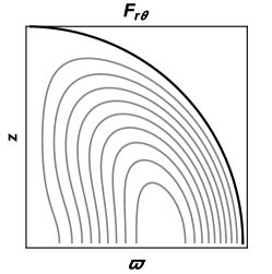
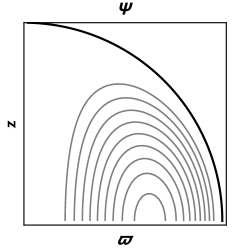
Figure 2: Equi–$F_{r\theta}$ contours (Left) and equi–$\Psi$ contours (Right) on the meridional cross section for the model with $\Gamma=2.05$ and $M/R=0.2$. Here, $z$ and $\varpi$ are defined by $z=r\cos\theta$ and $\varpi=r\sin\theta$, respectively. The thick quarter circle shows the surface of the star, on which $F_{r\theta}=0$ and $\Psi=0$ are required by the boundary condition.

The distribution of magnetic fields is completely determined by the two arbitrary functions, $\Psi(w)$ and $K(w)$, with $w$ being the function of the background quantities. For the two arbitrary functions, we have assumed equations (63) and (64) in this paper. In Figure 2, we give the profiles of magnetic fields: the toroidal magnetic field $F_{r\theta}$ and the poloidal flux function $\Psi$ for the background star with $\Gamma=2.05$ and $M/R=0.2$. The right of Figure 2 shows how lines of the magnetic force on the meridional cross section behave because an equi–$\Psi$ line corresponds to a line of the magnetic force. Note that there is no magnetic field outside the star in the model constructed in this study as mentioned before.

For investigating the effects of magnetic fields on the structure of the star, it is helpful to introduce the quantities that represent typical strength of the magnetic field of the star. The norms of the toroidal and poloidal magnetic fields are, respectively, given by

$$\left|{}^{(t)}B\right|^{2} = \varepsilon_{t}^{2}b^{2}r^{2}\sin^{2}\theta\,e^{2\nu}\left({}^{(0)}\rho^{(0)}h\right)^{2}\,,$$ (121)

$$\left|{}^{(p)}B\right|^{2} = \varepsilon_{p}^{2}a^{2}\,4e^{4\nu}\left({}^{(0)}\rho^{(0)}h\cos\theta\right)^{2}$$ (122)

$$+e^{4\nu-2\lambda}\sin^{2}\theta$$

$$\times\left\{r{d\over dr}\left({}^{(0)}\rho^{(0)}h\right)\right.$$

$$\left.\quad+2\left({}^{(0)}\rho^{(0)}h\right)\left(r{d\nu\over dr}+1\right)\right\}^{2}\,.$$

The maximum value of the norm of the toroidal magnetic field is then given by

$$\left|{}^{(t)}B_{\rm max}\right|^{2}=\varepsilon_{t}^{2}b^{2}\,{\rm max}\left[r^{2}\,e^{2\nu}\left({}^{(0)}\rho^{(0)}h\right)^{2}\right]\,,$$ (123)

where ${\rm max}\left[f(r)\right]$ means the maximum value of the function $f(r)$. The maximum value of the norm of the poloidal magnetic field is mostly attained at the center of the star. Thus, the norm of the poloidal magnetic field at the center of the star, given by

$$\left|{}^{(p)}B_{c}\right|^{2}=\varepsilon_{p}^{2}a^{2}\,4e^{4\nu(0)}\left({}^{(0)}\rho(0)^{(0)}h(0)\right)^{2}\,,$$ (124)

may be used as a representative value of the strength of the poloidal magnetic field. By using these values of the norms, we may obtain the two dimensionless quantities representing magnetic-field strength, given by

$${}^{(t)}{\cal R}_{M}={\left|{}^{(t)}B_{\rm max}\right|^{2}R^{4}\over 4M^{2}}\,,^{(p)}{\cal R}_{M}={\left|{}^{(p)}B_{c}\right|^{2}R^{4}\over 4M^{2}}\,,$$ (125)

which are as large as the ratios of the toroidal and the poloidal magnetic energies to the gravitational energy, respectively. The perturbations due to the magnetic field given in equation (34) basically depend on the dimensionless smallness parameters $\varepsilon_{t}$ and $\varepsilon_{p}$, which can be arbitrarily set depending on the desired magnetic field-strength as long as $1\gg\varepsilon_{t}\gg\varepsilon_{p}$. This arbitrariness in perturbation quantities is then removed by using the two dimensionless quantities ${}^{(t)}{\cal R}_{M}$ and ${}^{(p)}{\cal R}_{M}$ when numerical results are shown in this paper.

Figure 3: Normalized nondimensional changes in the gravitational mass $\Delta M/M{}^{(t)}{\cal R}_{M}$ and the baryon rest-mass $\Delta M^{*}/M^{*}{}^{(t)}{\cal R}_{M}$, given as functions of the central density of the background star ${}^{(0)}\rho(0)$. The solid circle indicates the result obtained within the framework of Newton’s dynamics and theory of gravity (cf., Appendix).

Figure 4: Normalized nondimensional changes in the internal thermal energy $\Delta E_{\rm int}/E_{\rm int}{}^{(t)}{\cal R}_{M}$, given as functions of the central density of the background star ${}^{(0)}\rho(0)$. The solid circle indicates the result obtained within the framework of Newton’s dynamics and theory of gravity (cf., Appendix).

Figure 5: Normalized nondimensional changes in the mean radius $(\Delta r)_{0}/R{}^{(t)}{\cal R}_{M}$, given as functions of the central density of the background star ${}^{(0)}\rho(0)$. The solid circle indicates the result obtained within the framework of Newton’s dynamics and theory of gravity (cf., Appendix).

Figure 6: Normalized nondimensional changes in the mass quadrupole moment $\Delta Q/MR^{2}{}^{(t)}{\cal R}_{M}$, given as functions of the central density of the background star ${}^{(0)}\rho(0)$. The solid circle indicates the result obtained within the framework of Newton’s dynamics and theory of gravity (cf., Appendix).

Figure 7: Normalized changes in the ellipticity $e^{*}/{}^{(t)}{\cal R}_{M}$, given as functions of the central density of the background star ${}^{(0)}\rho(0)$. The solid circle indicates the result obtained within the framework of Newton’s dynamics and theory of gravity (cf., Appendix).

Figure 8: Normalized nondimensional changes in the toroidal magnetic energy $E_{\rm EM}^{(t)}/\left|W\right|{}^{(t)}{\cal R}_{M}$, given as functions of the central density of the background star ${}^{(0)}\rho(0)$. The solid circle indicates the result obtained within the framework of Newton’s dynamics and theory of gravity (cf., Appendix).

Figure 9: Normalized nondimensional changes in the poloidal magnetic energy $E_{\rm EM}^{(p)}/\left|W\right|{}^{(p)}{\cal R}_{M}$, given as functions of the central density of the background star ${}^{(0)}\rho(0)$. The solid circle indicates the result obtained within the framework of Newton’s dynamics and theory of gravity (cf., Appendix).

Figure 10: Normalized changes in the nondimensional magnetic helicity ${\cal H}_{M}/\sqrt{{}^{(t)}{\cal R}_{M}{}^{(p)}{\cal R}_{M}}$, given as functions of the central density of the background star ${}^{(0)}\rho(0)$. The solid circle indicates the result obtained within the framework of Newton’s dynamics and theory of gravity (cf., Appendix).

First, we examine properties of the magnetized stars obtained under the condition of $\Delta\rho_{c}=0$, i.e., their central densities are kept constant when the magnetic fields are imposed. In Figure 3, normalized nondimensional changes in the gravitational mass $\Delta M\left/M{}^{(t)}{\cal R}_{M}\right.$ and the baryon rest-mass $\Delta M^{*}\left/M^{*}{}^{(t)}{\cal R}_{M}\right.$ are plotted as functions of the central density of the background star ${}^{(0)}\rho(0)$. In Figures 4 through 10, we plot, as functions of the central density of the background star ${}^{(0)}\rho(0)$, normalized nondimensional changes in the internal thermal energy $\Delta E_{\rm int}\left/E_{\rm int}{}^{(t)}{\cal R}_{M}\right.$, the mean radius $\left(\Delta r\right)_{0}\left/R{}^{(t)}{\cal R}_{M}\right.$, the mass quadrupole moment $\Delta Q\left/MR^{2}{}^{(t)}{\cal R}_{M}\right.$, the ellipticity $e^{*}\left/{}^{(t)}{\cal R}_{M}\right.$, the toroidal magnetic energy $E_{\rm EM}^{(t)}\left/|W|{}^{(t)}{\cal R}_{M}\right.$, and the poloidal magnetic energy $E_{\rm EM}^{(p)}\left/|W|{}^{(p)}{\cal R}_{M}\right.$, the magnetic helicity ${\cal H}_{M}\left/\sqrt{{}^{(t)}{\cal R}_{M}{}^{(p)}{\cal R}_{M}}\right.$, respectively. In Figures 3 through 10, the solid circles on the vertical axis indicate the results obtained by the calculation based on Newtonian magnetohydrodynamics and Newton’s theory of gravity (cf., Appendix). In these figures, we see that the present general relativistic results in the Newtonian limit (the limit of ${}^{(0)}\rho(0)\to 0$) are nicely agreement with those obtained by the Newtonian calculations. This fact serves as a useful consistency check of our numerical code.

Properties of the magnetized stars with $\Delta\rho_{c}=0$ observed in Figures 3 through 10 are summarized as follows: The results for the models with $\Gamma=2.05$ are little different from those for the models with $\Gamma=(n+1)/n\approx 1.95238$ (cf. Figures 3 through 10). This implies that small stratification has little effect on the equilibrium structure of the magnetized stars. The imposition of the toroidal magnetic fields results in a decrease in the total baryon rest-mass, i.e., $\Delta M^{*}<0$. Due to the imposition of the toroidal magnetic fields, values of the gravitational mass decrease, i.e., $\Delta M<0$, for the background stars with ${}^{(0)}\rho(0)\lessapprox 0.255$ while they increase, i.e., $\Delta M>0$, for the background stars with ${}^{(0)}\rho(0)\gtrapprox 0.255$ (cf. Figure 3). The mean radius of the star $\left(\Delta r\right)_{0}$ increases when the toroidal magnetic field is imposed (cf. Figure 5). The values of the mass quadrupole moment $\Delta Q$ and the ellipticity $e^{*}$ are negative, which reflects the fact that the star is prolate (cf. Figures 6 and 7). The prolate deformation is typical for stars containing dominant toroidal magnetic fields (cf., e.g., Refs kiuchi ; frieben ).

Table 2: Global and physical quantities.

$(\Gamma,M/R)$	$\displaystyle{\Delta\rho_{c}\over{}^{(0)}\rho(0){}^{(t)}{\cal R}_{M}}$	$\displaystyle{\Delta M\over M{}^{(t)}{\cal R}_{M}}$	$\displaystyle{\Delta E_{\rm int}\over E_{\rm int}{}^{(t)}{\cal R}_{M}}$	$\displaystyle{(\Delta r)_{0}\over R{}^{(t)}{\cal R}_{M}}$	$\displaystyle{\Delta Q\over MR^{2}{}^{(t)}{\cal R}_{M}}$	$\displaystyle{e^{*}\over{}^{(t)}{\cal R}_{M}}$	$\displaystyle{E_{\rm EM}^{(t)}\over|W|{}^{(t)}{\cal R}_{M}}$	$\displaystyle{E_{\rm EM}^{(p)}\over|W|{}^{(p)}{\cal R}_{M}}$	$\displaystyle{{\cal H}_{M}\over\sqrt{{}^{(t)}{\cal R}_{M}{}^{(p)}{\cal R}_{M}}}$
(1.95238,0.1)	0.2424	$1.565\times 10^{-2}$	$-0.2413$	0.3048	$-0.1105$	$-0.2294$	0.2097	$9.747\times 10^{-2}$	1.512
(1.95238,0.2)	0.8077	$2.338\times 10^{-2}$	0.4077	$-1.607\times 10^{-2}$	$-3.946\times 10^{-2}$	$-0.1213$	0.1626	$7.349\times 10^{-2}$	1.596
(2.05,0.1)	0.2457	$1.646\times 10^{-2}$	$-0.2397$	0.3056	$-0.1116$	$-0.2316$	0.2110	$9.904\times 10^{-2}$	1.527
(2.05,0.2)	0.5677	$2.257\times 10^{-2}$	0.2043	$8.193\times 10^{-2}$	$-4.134\times 10^{-2}$	$-0.1271$	0.1672	$7.792\times 10^{-2}$	1.654

Next, we examine properties of the magnetized stars obtained under the condition of $\Delta M^{*}=0$, i.e., their total baryon rest-masses are kept constant when the magnetic fields are imposed. Table 2 lists global and physical quantities characterizing the magnetized stars with $\Delta M^{*}=0$; the changes in the central density $\Delta\rho_{c}$, the gravitational mass $\Delta M$, the internal thermal energy $\Delta E_{\rm int}$, the mean radius $\left(\Delta r\right)_{0}$, the mass quadrupole moment $\Delta Q$, the ellipticity $e^{*}$, the toroidal magnetic energy $E_{\rm EM}^{(t)}$, the poloidal magnetic energy $E_{\rm EM}^{(p)}$, and the magnetic helicity ${\cal H}$. In this table, all the quantities are normalized to be nondimensional, as given in the first row.

Properties of the magnetized star with $\Delta M^{*}=0$ observed in Table 2 are summarized as follows: The imposition of the toroidal magnetic fields results in an increase in the central density, i.e., $\Delta\rho_{c}>0$. The values of the mass quadrupole moment $\Delta Q$ and the ellipticity $e^{*}$ are negative, which reflects the fact that the star is prolate. These properties concerning $\Delta\rho_{c}$ and $\Delta Q$ are attributed to the magnetic hoop stress around the symmetry axis due to the toroidal magnetic field, which tends to make the star prolate like a rubber belt fastening around the waist of a star. The gravitational mass increase due to the imposition of the toroidal magnetic fields, i.e., $\Delta M>0$.

Since the deformation of the star considered in this study is caused by toroidal magnetic fields only, even though poloidal magnetic fields make the deformation of the spacetime, the results obtained in this study can be compared with those obtained by Kiuchi and Yoshida kiuchi , who derived general relativistic stars having purely toroidal magnetic fields with a non-perturbative approach. Although weakly magnetized stars cannot be calculated with Kiuchi and Yoshida’s method because of their non-perturbative approach, it is found that the present results are consistent with those obtained by Kiuchi and Yoshida kiuchi (Compare, e.g., Table 2 with Figure 6 of Ref. kiuchi ).

V Discussion

In this study, as mentioned before, the general relativistic magnetized stars are constructed under the condition of $\varepsilon_{p}\ll\varepsilon_{t}\ll 1$, and the effects of magnetic fields are investigated within accuracy $O\left(\varepsilon_{t}\varepsilon_{p}\right)$. The terms higher than $O\left(\varepsilon_{p}^{2}\right)$ in the equations are then discarded. The deformation of the star and spacetime occurs in the $\varepsilon_{t}^{2}$-order, which is attributed to the magnetic effects due to the toroidal field. This deformation due to the toroidal magnetic field is the same as that of the weakly magnetized star with purely toroidal fields within accuracy $O\left(\varepsilon_{t}^{2}\right)$. Thus, the present results include those for the weakly magnetized star with purely toroidal fields. To our knowledge, such general relativistic magnetized stars having purely toroidal fields have been constructed with a perturbative approach for the first time. The $\varepsilon_{t}\varepsilon_{p}$-order effects appear in the deformation of the spacetime only. Therefore, the $\varepsilon_{t}\varepsilon_{p}$-order effects are general relativistic ones and disappear in Newton’s dynamics and theory of gravity. Within the framework of Newtonian magnetohydrodynamics, in other words, the poloidal magnetic field does not affect the deformation of the star within accuracy $O\left(\varepsilon_{t}\varepsilon_{p}\right)$ (cf. Appendix). From a general relativistic point of view, an interesting fact is that the $\varepsilon_{t}\varepsilon_{p}$-order effects violate the circularity conditions (cf. equation (62)). As a result, the $r\varphi$-component of the metric $g_{r\varphi}$ appears inside the star (cf. equation (83)).

In this paper, we have shown that stationary and axisymmetric solutions of the magnetized star with mixed poloidal-toroidal fields may indeed be constructed within accuracy $O\left(\varepsilon_{t}\varepsilon_{p}\right)$. However, such stationary and axisymmetric solutions cannot be constructed if the $\varepsilon_{p}^{2}$-order effects on the structure of the star are included. The reason for this is the following: The $\varepsilon_{p}^{2}$-order equations are the same as those for the weakly magnetized star with purely poloidal fields within accuracy $O\left(\varepsilon_{p}^{2}\right)$. For the weakly magnetized star with purely poloidal fields, the poloidal flux function $\Psi$ has to satisfy the general relativistic version of the so-called Grad-Shafranov equation (cf., e.g., Ref. konno ). In the present approximation, however, the flux function $\Psi$ has to be given by the arbitrary function of the background quantity $w=^{(0)}\rho^{(0)}he^{2\nu}r^{2}\sin^{2}\theta$ (cf. equations (39) and (40)). The flux function $\Psi$ given by the arbitrary function of $w$ does not, in general, fulfill the Grad-Shafranov equation. Therefore, the $\varepsilon_{p}^{2}$-order equations cannot be solved consistently with the lower-order equations. This implies that the weakly magnetized stars constructed in this study cannot be stationary and axisymmetric when the condition of $\varepsilon_{p}\ll\varepsilon_{t}$ is violated.

After obtaining equilibrium models of stars, check of their stability is an important issue because unstable solutions lose their physical meaning in the sense that they are not realized in nature. Since magnetized stars with purely toroidal fields are unstable, the present magnetized star models are indeed unstable when we set $\varepsilon_{p}=0$, which corresponds to the case of purely toroidal fields. As mentioned in Introduction, both a stable stratification of the fluid and poloidal magnetic fields act as stabilizing agents of the toroidal magnetic fields inside the star. The stably stratified stars with $1\gg\varepsilon_{t}\gg\varepsilon_{p}\neq 0$ constructed in this study are therefore possibly stable. As mentioned before, unfortunately, reliable and useful procedures for the diagnosis of the stability for the magnetized star have not yet been established. (For the moment, numerical simulations will be the most reliable way to check the stability, but they are tough work.) Although we are not sure that it is adaptive for the present magnetized star models, Braithwaite’s stability condition, given in equation (1), is available to assess their stability. If a magnetized star characterized by $\Gamma=2.05$, $R\approx 10$ km, $M\approx 1.4\,M_{\odot}$, and ${}^{(t)}B_{\rm max}\approx 10^{15}$ G is considered, we have ${}^{(t)}{\cal R}_{M}\approx 5\times 10^{-7}$ and $E^{(t)}_{\rm EM}/|W|\approx 8\times 10^{-8}$. We then obtain Braithwaite’s stability condition for the model, given by

$$8\times 10^{-5}\lesssim{E_{\rm EM}^{(p)}\over E_{\rm EM}^{(t)}}\lesssim 0.8\,,$$ (126)

where $E_{\rm EM}^{(p)}/E_{\rm EM}\approx E_{\rm EM}^{(p)}/E_{\rm EM}^{(t)}$ is used, and $\tilde{a}\approx 10^{3}$ is assumed because the star is a stably stratified neutron star model. For the model considered, we have $E_{\rm EM}^{(p)}/E_{\rm EM}^{(t)}\approx 0.5\,{\cal R}_{M}^{(p)}/{\cal R}_{M}^{(t)}$. Braithwaite’s stability condition for the model then becomes

$$1.6\times 10^{-4}\lesssim{{\cal R}_{M}^{(p)}\over{\cal R}_{M}^{(t)}}\lesssim 1.6\,.$$ (127)

Under the condition of $\varepsilon_{p}\ll\varepsilon_{t}\ll 1$, which is the basic assumption in this study, we can appropriately choose vales of ${{\cal R}_{M}^{(p)}/{\cal R}_{M}^{(t)}}$ so as to satisfy the inequality given in equation (127), Braithwaite’s stability condition for the model. Therefore, the present magnetized star models satisfying the inequality (127) are stable if Braithwaite’s stability condition is properly adaptive for them. In order to examine stability properly, however, we have to make stability analyses by using dynamical simulations or solving linear eigenvalue problems, which exceed the scope of this work and remain as future challenges.

VI Summary

We have constructed the stably stratified magnetized stars within the framework of general relativity. The effects of magnetic fields on the structure of the star and spacetime are treated as perturbations of non-magnetized stars. By assuming ideal magnetohydrodynamics and employing one-parameter equations of state, we derive basic equations for describing stationary and axisymmetric stably stratified stars containing magnetic fields whose toroidal components are much larger than the poloidal ones. A number of the polytropic models are numerically calculated to investigate basic properties of the effects of magnetic fields on the stellar structure. According to the stability result obtained by Braithwaite, which remains a matter of conjecture for general magnetized stars, certain of the magnetized stars constructed in this study are possibly stable.

Appendix A Newtonian analysis

In this appendix, we present the Newtonian version of the magnetized star considered in this study. The results of the Newtonian analysis can be used to compare to those of the general relativistic analysis in the Newtonian limit. We may then check consistency between them. Similar analyses to those given in this appendix are found in, e.g., Refs. sinha ; asai .

Within the framework of Newtonian magnetohydrodynamics, the dynamics of perfectly conductive fluids may be described by the following equations:

$$\partial_{t}\,\rho+\nabla_{a}\left(\rho\,v^{a}\right)=0\,,$$ (128)

$$\nabla_{a}B^{a}=0\,,$$ (129)

$$\partial_{t}\,B^{a}=\nabla_{b}\left(v^{a}B^{b}-v^{b}B^{a}\right)\,,$$ (130)

$$\left(\partial_{t}+v^{b}\nabla_{b}\right)v_{a} = -{1\over\rho}\nabla_{a}p-\nabla_{a}\Phi$$ (131)

$$+ {1\over 4\pi\rho}\left(B^{b}\nabla_{b}B_{a}-B^{b}\nabla_{a}B_{b}\right)\,,$$

$$\nabla^{b}\nabla_{b}\Phi=4\pi G\rho\,,$$ (132)

where $\rho$, $v^{a}$, $B^{a}$, $p$, and $\Phi$ are the mass density, the fluid velocity, the magnetic field, the pressure, and the gravitational potential, respectively. Here, $\nabla_{a}$ denotes the covariant derivative associated with the metric $g_{ab}$, and spatial indices are denoted by lower case Roman letters ($a,b,c,\cdots$).

Following the assumptions given in Sec. III, we assume that there is no fluid flow, i.e.,

$$v^{a}=0\,,$$ (133)

and that the magnetized stars are stationary and axisymmetric. Therefore, physical quantities associated with the magnetized star are independent of the time coordinate $t$ and the azimuthal angle about the symmetry axis $\varphi$. Under the assumption of stationarity and axisymmetry, the magnetic fields $B^{a}$ may, in terms of two functions $B$ and $A_{\varphi}$ independent of $t$ and $\varphi$, be written by

$$\quad B^{a}=B\varphi^{a}+\epsilon^{ab\varphi}\partial_{b}A_{\varphi}\,,$$ (134)

where $\varphi^{a}$ denotes the rotational Killing vector, $\epsilon^{abc}$ is the contravariant spatial Levi-Civita tensor, and $A_{\varphi}$ is the $\varphi$-component of the vector potential $A_{a}$ or the poloidal flux function. Due to the assumptions given in equations (133) and (134), equations (128)–(130) are satisfied automatically, and the $\varphi$-component of equation (131) becomes

$${1\over 4\pi\rho}\left(B^{b}\nabla_{b}B_{\varphi}-B^{b}\nabla_{\varphi}B_{b}\right) = {1\over 4\pi\rho}\epsilon^{bc\varphi}\partial_{c}A_{\varphi}\partial_{b}\left(B\,\varphi_{\varphi}\right)$$ (135)

$$= 0\,.$$

Therefore, the function $B$ has to be given in terms of an arbitrary function $K(A_{\varphi})$ by

$$B={K(A_{\varphi})\over\varphi_{\varphi}}\,.$$ (136)

By using equation (136), we may rewrite the poloidal components of the Lorentz force term in equation (131) as follows:

$${1\over 4\pi\rho}\left(B^{b}\nabla_{b}B_{C}-B^{b}\nabla_{C}B_{b}\right)=-{K\over 4\pi\rho\,\varphi_{\varphi}}\partial_{C}K$$

$$\quad\quad\quad\quad-{1\over 4\pi\rho\sqrt{g}}\left(\partial_{C}A_{\varphi}\right)\left(\partial_{2}B_{1}-\partial_{1}B_{2}\right)\,,$$ (137)

where the index $C$ denote the poloidal indices, i.e., $C=1,2$, and $g$ means the determinant of the metric $g_{ab}$. If we make the same approximation as that used in Sec. III, the first and the second terms in the right-hand side of equation (137) are $O\left(\varepsilon_{t}^{2}\right)$ and $O\left(\varepsilon_{p}^{2}\right)$, respectively. Under the assumption of $\varepsilon_{p}\ll\varepsilon_{t}\ll 1$, equation (137) becomes

$${1\over 4\pi\rho}\left(B^{b}\nabla_{b}B_{C}-B^{b}\nabla_{C}B_{b}\right)=-{K\over 4\pi\rho\,\varphi_{\varphi}}\partial_{C}K+O\left(\varepsilon_{t}\varepsilon_{p}\right)\,,$$ (138)

within accuracy $O\left(\varepsilon_{t}\varepsilon_{p}\right)$. In other words, similarly to the general relativistic case, poloidal magnetic fields do not affect the deformation of the star within accuracy $O\left(\varepsilon_{t}\varepsilon_{p}\right)$. The Euler equation then becomes

$${1\over\rho}\nabla_{C}p+\nabla_{C}\Phi+{1\over 8\pi\rho\,\varphi_{\varphi}}\partial_{C}K^{2}+O\left(\varepsilon_{t}\varepsilon_{p}\right)=0\,.$$ (139)

This equation may be integrable if the following conditions for the three functions $p$, $K$, and $A_{\varphi}$, are assumed:

$$p=p(\rho)\,,\quad K=K(\rho\varphi_{\varphi})\,,\quad A_{\varphi}=A_{\varphi}(\rho\varphi_{\varphi})\,.$$ (140)

After giving the actual forms of the three functions $p$, $K$, and $A_{\varphi}$, we may then obtain the weakly magnetized star models with mixed poloidal and toroidal fields.

In what follows, the spherical polar coordinates $(r,\theta,\varphi)$ are used in order to derive the master equations for the weakly magnetized stars with mixed poloidal-toroidal fields. The metric is then given by

$$ds^{2}=dr^{2}+r^{2}d\theta^{2}+r^{2}\sin^{2}\theta d\varphi^{2}\,.$$ (141)

The rotational Killing vector $\varphi_{a}$ is given by

$$\varphi_{a}=(0,0,r^{2}\sin^{2}\theta)\,.$$ (142)

Following the assumptions given in Sec. III, we set the two arbitrary functions $K$ and $A_{\varphi}$ as follows:

$$K = {B_{c}\over\sqrt{2}\,\rho_{c}\alpha}\,\rho\,r^{2}\sin^{2}\theta\,,$$ (143)

$$A_{\varphi} = b\rho\,r^{2}\sin^{2}\theta\,,$$ (144)

where $B_{c}$, $\rho_{c}$, and $\alpha$ are constants that are related to the magnetic field strength, density, and radius of the star, respectively, and $b$ is a constant. The absolute value of the magnetic field $B^{a}$ is then given by

$$\sqrt{B^{a}B_{a}}={B_{c}\over\sqrt{2}}\,\hat{\rho}\,\xi\sin\theta+O\left(\varepsilon_{p}^{2}\right)\,,$$ (145)

where the two dimension-less quantities $\hat{\rho}=\rho/\rho_{c}$ and $\xi=r/\alpha$ are introduced. By using equation (143), we may rewrite equation (139) as

$$\nabla_{a}p=-\rho\nabla_{a}\Psi\,,$$ (146)

$$\Psi=\Phi+{1\over 3}\,\Omega_{A}^{2}r^{2}\,\hat{\rho}\left\{1-P_{2}\left(\cos\theta\right)\right\}-\Phi_{0}\,,$$ (147)

where $\Omega_{A}$ is the Alfvèn frequency, defined by $\displaystyle\Omega_{A}=\sqrt{{B_{c}^{2}\over 4\pi\rho_{c}\alpha^{2}}}$, and $\Phi_{0}$ is a constant. Since $\Omega_{A}=O\left(\varepsilon_{t}\right)$, within accuracy $O\left(\varepsilon_{t}\varepsilon_{p}\right)$, the function $\Psi$ fulfills the equation, given by

$$\nabla^{a}\nabla_{a}\Psi = 4\pi G\rho$$ (148)

$$+ {1\over 3}\,\Omega_{A}^{2}\left\{r^{2}{d^{2}\hat{\rho}_{0}\over dr^{2}}+6r{d\hat{\rho}_{0}\over dr}+6\hat{\rho}_{0}\right.$$

$$\left.-\left(r^{2}{d^{2}\hat{\rho}_{0}\over dr^{2}}+6r{d\hat{\rho}_{0}\over dr}\right)P_{2}\left(\cos\theta\right)\right\}$$

$$+O\left(\varepsilon_{p}^{2}\right)\,,$$

where $\hat{\rho}_{0}$ is the dimensionless density of the non-magnetized star normalized by its central value. The function $\Psi$ may be expanded in terms of the parameter $\Omega_{A}$, and then written by

$$\Psi\left(r,\theta\right) = \Psi_{0}\left(r\right)$$ (149)

$$- 2\alpha^{2}\Omega_{A}^{2}\left[\psi_{0}\left(r\right)+\psi_{2}\left(r\right)P_{2}\left(\cos\theta\right)\right]$$

$$+O\left(\varepsilon_{p}^{2}\right)\,,$$

where $\Psi_{0}$ means the function $\Psi$ for the non-magnetized star. Since we have $p=p(\rho)$ and equation (146), the density $\rho$ is a function of $\Psi$. Therefore, the density $\rho$ may be also expanded in terms of the parameter $\Omega_{A}$, and then written by

$$\rho\left(r,\theta\right) = \rho_{0}\left(r\right)$$ (150)

$$- 2\alpha^{2}\Omega_{A}^{2}{d\rho_{0}\over d\Psi_{0}}\left[\psi_{0}\left(r\right)+\psi_{2}\left(r\right)P_{2}\left(\cos\theta\right)\right]$$

$$+O\left(\varepsilon_{p}^{2}\right)\,,$$

where $\rho_{0}$ means the density $\rho$ for the non-magnetized star. Instituting equations (149) and (150) into equation (148), we obtain

$$\alpha^{2}\nabla^{a}\nabla_{a}\Psi_{0}\left(r\right)=4\pi G\alpha^{2}\rho_{0}\left(r\right)\,,$$ (151)

$${1\over\xi^{2}}{d\over d\xi}\left(\xi^{2}\,{d\psi_{0}\over d\xi}\right) = k(\xi)\psi_{0}$$ (152)

$$- {1\over 6r^{2}}{d\over dr}\left(r^{2}{d\over dr}\left(r^{2}\hat{\rho}_{0}\right)\right)\,,$$

$${1\over\xi^{2}}{d\over d\xi}\left(\xi^{2}\,{d\psi_{2}\over d\xi}\right) = \left(k\left(\xi\right)+{6\over\xi^{2}}\right)\psi_{2}$$ (153)

$$+ {1\over 6}\left(r^{2}{d^{2}\hat{\rho}_{0}\over dr^{2}}+6r{d\hat{\rho}_{0}\over dr}\right)\,,$$

where

$$k\left(\xi\right)=4\pi G\alpha^{2}{d\rho_{0}\over d\Psi_{0}}\,.$$ (154)

In order to solve the three ordinary differential equations (151)–(153), boundary conditions at the center and surface of the star are necessary. We require that physical quantities are regular near the center of the star and that values of the central density are independent of the magnetic field-strength. At the center of the star, therefore, we have

$${d\Psi_{0}\over d\xi}\left(0\right)=0\,,\quad\psi_{0}\left(0\right)=0\,,\quad{d\psi_{0}\over d\xi}\left(0\right)=0\,,$$

$$\psi_{2}\left(0\right)=0\,,\quad{d\psi_{2}\over d\xi}\left(0\right)=0\,.$$ (155)

To determine the boundary condition at the surface of the star, we need the equation of the surface of the star, given by

$$r=R\left(1+\delta\zeta\right)+O\left(\varepsilon_{p}^{2}\right)\,,$$ (156)

where $R$ is the radius for the non-magnetized star. The dimensionless displacement $\delta\zeta$ is given by

$$\delta\zeta={2\alpha^{2}\Omega_{A}^{2}\over\displaystyle R{d\Psi_{0}\over dr}(R)}\left[\psi_{0}\left(\xi_{1}\right)+\psi_{2}\left(\xi_{1}\right)P_{2}\left(\cos\theta\right)\right]\,,$$ (157)

where $\xi_{1}=R/\alpha$. The displacement $\delta\zeta$ is used to evaluate the ellipticity of the surface of the star $e^{*}$, defined by

$$e^{*} = {R\left(1+\delta\zeta\left(\pi/2\right)\right)-R\left(1+\delta\zeta\left(0\right)\right)\over R}$$ (158)

$$= -{3\over 2}2\alpha^{2}\Omega_{A}^{2}{1\over\displaystyle R{d\Psi_{0}\over dr}(R)}\psi_{2}\left(\xi_{1}\right)\,.$$

The gravitational potentials inside and outside the star within accuracy $O\left(\varepsilon_{t}^{2}\right)$ are, respectively, given by

$$\Phi = \Psi_{0}\left(r\right)+c_{0}$$ (159)

$$- 2\alpha^{2}\Omega_{A}^{2}\left[c_{1,0}+\psi_{0}\left(\xi\right)+\psi_{2}\left(\xi\right)P_{2}\left(\cos\theta\right)\right]$$

$$- {1\over 3}\,\Omega_{A}^{2}r^{2}\,\hat{\rho}\left\{1-P_{2}\left(\cos\theta\right)\right\}\,,$$

and

$$\Phi=-{\kappa_{0}\over\xi}-2\alpha^{2}\Omega_{A}^{2}\left[{\kappa_{1,0}\over\xi}+{\kappa_{1,2}\over\xi^{3}}P_{2}\left(\cos\theta\right)\right]\,,$$ (160)

where $c_{0}$, $c_{1,0}$, $\kappa_{0}$, $\kappa_{1,0}$ and $\kappa_{1,2}$ are constants. Since the gravitational potential and its derivative have to be continuous at the surface of the star, we obtain the following relations:

$$\kappa_{0}=\xi_{1}^{2}\partial_{\xi}\Psi_{0}\left(R\right)\,,\ c_{0}=-\Psi_{0}\left(R\right)-\xi_{1}\partial_{\xi}\Psi_{0}\left(R\right)\,,$$ (161)

$$-c_{1,0}=-{\kappa_{1,0}\over\xi_{1}}+\psi_{0}\left(\xi_{1}\right)\,,\quad{\kappa_{1,2}\over\xi_{1}^{3}}=\psi_{2}\left(\xi_{1}\right)\,,$$ (162)

$${\kappa_{1,0}\over\xi_{1}^{2}}=-{d\psi_{0}\over d\xi}(\xi_{1})-{1\over 6}\,\xi_{1}^{2}{d\hat{\rho}\over d\xi}\left(\xi_{1}\right)\,,$$

$$3{\kappa_{1,2}\over\xi_{1}^{4}}=-{d\psi_{2}\over d\xi}(\xi_{1})+{1\over 6}\,\xi_{1}^{2}{d\hat{\rho}\over d\xi}\left(\xi_{1}\right)\,.$$ (163)

For equations (151) and (152), therefore, boundary conditions are not imposed at the surface of the star, and instead the constants characterizing the gravitational potential are determined through equation (161) and

$$\kappa_{1,0} = -\xi_{1}^{2}{d\psi_{0}\over d\xi}(\xi_{1})-{1\over 6}\,\xi_{1}^{4}{d\hat{\rho}\over d\xi}\left(\xi_{1}\right)\,,$$

$$c_{1,0} = -\psi_{0}(\xi_{1})-\xi_{1}{d\psi_{0}\over d\xi}(\xi_{1})-{1\over 6}\,\xi_{1}^{3}{d\hat{\rho}\over d\xi}\left(\xi_{1}\right)\,,$$ (164)

As for equation (153), the boundary condition at the surface of the star is given by

$$3\psi_{2}\left(\xi_{1}\right)+\xi_{1}{d\psi_{2}\over d\xi}\left(\xi_{1}\right)={1\over 6}\,\xi_{1}^{3}{d\hat{\rho}\over d\xi}\left(\xi_{1}\right)\,.$$ (165)

The constant related to the mass quadrupole moment $\kappa_{1,2}$ is determined through

$$\kappa_{1,2}=\xi_{1}^{3}\psi_{2}\left(\xi_{1}\right)\,.$$ (166)

Following the assumptions given in Sec. III, we assume the polytropic equation of state, given by

$$p=\kappa\rho^{1+{1\over n}}\,,$$ (167)

where $\kappa$ and $n$ are constants. Introducing the Lane-Emden function $\Theta$, then, we may write $\rho$ and $p$ as

$$\rho=\rho_{c}\Theta^{n}\,,\quad p=p_{c}\Theta^{n+1}\,,$$ (168)

where $\rho_{c}$ and $p_{c}$ are values of the density and pressure at the center of the star, respectively. The central pressure value $p_{c}$ is given in terms of $\rho_{c}$, $\kappa$, and $n$ by $p_{c}=\kappa\rho_{c}^{1+{1\over n}}$. Equation (151) is rewritten by

$${1\over\xi^{2}}{\partial\over\partial\xi}\left(\xi^{2}{\partial\over\partial\xi}\widehat{\Psi}\right)=\Theta^{n}\,,$$ (169)

where $\widehat{\Psi}$ is the dimensionless quantity, defined by

$$\widehat{\Psi}={\Psi\over 4\pi G\rho_{c}\alpha^{2}}\,.$$ (170)

From equation (146), inside the star, we obtain

$$\widehat{\Psi}=-\Theta+C\,,$$ (171)

where $C$ is a constant, and we set

$$\alpha=\sqrt{{(n+1)K\rho_{c}^{{1\over n}}\over 4\pi G\rho_{c}}}=\sqrt{{(n+1)p_{c}\over 4\pi G\rho_{c}^{2}}}\,.$$ (172)

Substituting equation (171) into equation (169) yields the Lane-Emden equation, given by

$${d^{2}\Theta\over d\xi^{2}}+{2\over\xi}{d\Theta\over d\xi}=-\Theta^{n}\,.$$ (173)

At the center of the star, the boundary conditions for equation (173) are, due to equations (155) and (168), given by

$$\Theta=1\,,\quad{d\Theta\over d\xi}=0\,,\quad{\rm at}\ \xi=0\,.$$ (174)

The function $k(\xi)$, defined in equation (154), is rewritten by

$$k\left(\xi\right)=-n\,\Theta^{n-1}\,.$$ (175)

Now that we obtain the complete set of equations for the weakly magnetized star with mixed poloidal-toroidal fields within the framework of Newtonian magnetohydrodynamics, which are composed of equations  (173), (152), and (153), we may construct the magnetized stars.

In order to investigate properties of equilibrium solutions of the magnetized star, global quantities are frequently used. The mass of the star $M$ is given by

$$M = 2\pi\int\rho r^{2}\sin\theta drd\theta\,,$$ (176)

$$= M_{0}\left(1+{\Delta M\over M_{0}}\right)+O\left(\varepsilon_{t}^{2}\right)\,,$$

where $M_{0}$ is the mass of the non-magnetized star, given by

$$M_{0}=-4\pi\alpha^{3}\rho_{c}\left.\xi_{1}^{2}{d\Theta\over d\xi}\right|_{\xi=\xi_{1}}\,,$$ (177)

and $\displaystyle{\Delta M\over M_{0}}$ is the normalized dimensionless change in the mass of the star, given by

$${\Delta M\over M_{0}}={\displaystyle{\Omega_{A}^{2}\over 2\pi G\rho_{c}}\left\{\left.{d\psi_{0}\over d\xi}\right|_{\xi=\xi_{1}}+{1\over 6}\left.\xi_{1}^{2}{d\hat{\rho}_{0}\over d\xi}\right|_{\xi=\xi_{1}}\right\}\over\displaystyle\left.{d\Theta\over d\xi}\right|_{\xi=\xi_{1}}}\,.$$ (178)

The internal thermal energy of the star $E_{\rm int}$ is given by

$$E_{\rm int} = 2\pi\int\rho\varepsilon r^{2}\sin\theta drd\theta\,,$$ (179)

$$= \left(E_{\rm int}\right)_{0}\left(1+{\Delta E_{\rm int}\over\left(E_{\rm int}\right)_{0}}\right)+O\left(\varepsilon_{t}^{2}\right)\,,$$

where $\left(E_{\rm int}\right)_{0}$ is the internal thermal energy of the non-magnetized star, given by

$$\left(E_{\rm int}\right)_{0}={4\pi\over\Gamma-1}{4\pi G\rho_{c}^{2}\alpha^{5}\over n+1}\int_{0}^{\xi_{1}}\Theta^{n+1}\xi^{2}d\xi\,,$$ (180)

and $\displaystyle{\Delta E_{\rm int}\over\left(E_{\rm int}\right)_{0}}$ is the normalized dimensionless change in the internal thermal energy of the star, given by

$${\Delta E_{\rm int}\over\left(E_{\rm int}\right)_{0}}={\displaystyle{\Omega_{A}^{2}\over 4\pi G\rho_{c}}2\left(n+1\right)\int_{0}^{\xi_{1}}\Theta^{n}\psi_{0}\left(r\right)\xi^{2}d\xi\over\displaystyle\int_{0}^{\xi_{1}}\Theta^{n+1}\xi^{2}d\xi}\,.$$ (181)

Here, the gamma-law equation of state, given in equation (113), is used. An average change in the radius of the star $\left(\Delta r\right)_{0}$, defined in equation (105), is given by

$${\left(\Delta r\right)_{0}\over R}=-2\Omega_{A}^{2}{\psi_{0}\left(\xi_{1}\right)\over\displaystyle 4\pi G\rho_{c}\xi_{1}\left.{d\Theta\over d\xi}\right|_{\xi=\xi_{1}}}\,.$$ (182)

The ellipticity associated with the surface shape of the star $e^{*}$ is explicitly given by

$$e^{*}=3\Omega_{A}^{2}{\psi_{2}\left(\xi_{1}\right)\over\displaystyle 4\pi G\rho_{c}\xi_{1}\left.{d\Theta\over d\xi}\right|_{\xi=\xi_{1}}}\,.$$ (183)

The mass quadrupole moment of the star $\Delta Q$ is, in terms of $\kappa_{1,2}$, given by

$${\Delta Q\over M_{0}R^{2}}=-{2\alpha^{2}\Omega_{A}^{2}\alpha^{3}\kappa_{1,2}\over\alpha\kappa_{0}\alpha^{2}\xi_{1}^{2}}\,.$$ (184)

The toroidal magnetic energy ${}^{(t)}E_{\rm EM}$ and the poloidal magnetic energy ${}^{(p)}E_{\rm EM}$ are, respectively, defined by

$${}^{(t)}E_{\rm EM}={1\over 8\pi}\int B^{\varphi}B_{\varphi}dV\,,$$

$${}^{(p)}E_{\rm EM}={1\over 8\pi}\int B^{C}B_{C}dV\,.$$ (185)

Then, the ratios of the toroidal and the poloidal magnetic energies to the unperturbed gravitational energy of the star $\displaystyle{{}^{(t)}E_{\rm EM}\over\left(\left|W\right|\right)_{0}}$ and $\displaystyle{{}^{(p)}E_{\rm EM}\over\left(\left|W\right|\right)_{0}}$ are, respectively, given by

$${{}^{(t)}E_{\rm EM}\over\left(\left|W\right|\right)_{0}}={\displaystyle{\Omega_{A}^{2}\over 3\cdot 4\pi\rho_{c}G}\int_{0}^{\xi_{1}}\hat{\rho}^{2}\xi^{4}d\xi\over\displaystyle-\int_{0}^{\xi_{1}}\hat{\rho}\widehat{\Phi}\xi^{2}d\xi}\,,$$ (186)

and

$${{}^{(p)}E_{\rm EM}\over\left(\left|W\right|\right)_{0}}={b^{2}\over 3\cdot 2\pi\alpha^{2}4\pi G}$$

$$\quad\quad\times{\displaystyle\int_{0}^{\xi_{1}}\left\{\left(\xi{d\hat{\rho}\over d\xi}+2\hat{\rho}\right)^{2}+2\rho^{2}\right\}\xi^{2}d\xi\over\displaystyle-\int_{0}^{\xi_{1}}\hat{\rho}\widehat{\Phi}\xi^{2}d\xi}\,,$$ (187)

where the unperturbed gravitational energy of the star $\left(\left|W\right|\right)_{0}$ is given by

$$\left(\left|W\right|\right)_{0} = -{1\over 2}\int\rho_{0}\Phi_{0}dV\,,$$ (188)

$$= -2\pi\alpha^{5}\rho_{c}^{2}4\pi G\int_{0}^{\xi_{1}}\hat{\rho}_{0}\widehat{\Phi}_{0}\xi^{2}d\xi\,.$$

The dimensionless magnetic helicity of the star ${\cal H}_{M}$ is given by

$${\cal H}_{M} = {{\cal H}\over GM_{0}^{2}}\,,$$ (189)

$$= {\displaystyle{bB_{c}\over\sqrt{2}\,3\pi G\alpha^{2}\rho_{c}}\int_{0}^{\xi_{1}}\hat{\rho}^{2}\xi^{4}d\xi\over\displaystyle\left(\left.\xi_{1}^{2}{d\Theta\over d\xi}\right|_{\xi=\xi_{1}}\right)^{2}}\,,$$

where ${\cal H}$ is the magnetic helicity of the star, defined by ${\cal H}=\int A_{a}B^{a}dV$.

Since the effects of magnetic fields on the structure of the star are treated as perturbations of the non-magnetized star, the solutions constructed in this study are inherently independent of the magnetic-field strength. However, the representation for the global and physical quantities defined before are dependent on the magnetic-field strength. In order to remove their field-strength dependence, following the treatment used in Sec. IV, we introduce the two dimensionless quantities representing magnetic-field strength, given by

$${}^{(t)}{\cal R}_{M} = {{}^{(t)}B_{\rm max}^{2}R^{4}\over 4GM^{2}}\,,$$ (190)

$$= {\left({\rm max}\left[\hat{\rho}\xi\right]\right)^{2}\over\displaystyle 8\left(\left.{d\Theta\over d\xi}\right|_{\xi=\xi_{1}}\right)^{2}}{\Omega_{A}^{2}\over 4\pi G\rho_{c}}\,,$$

$${}^{(p)}{\cal R}_{M} = {{}^{(p)}B_{c}^{2}R^{4}\over 4GM^{2}}\,,$$ (191)

$$= {b^{2}\over\displaystyle G\left(4\pi\right)^{2}\alpha^{2}\left(\left.{d\Theta\over d\xi}\right|_{\xi=\xi_{1}}\right)^{2}}\,,$$

where ${}^{(t)}B_{\rm max}$ is the maximum absolute value of the toroidal magnetic field inside the star, ${\rm max}[f]$ means the maximum value of the function $f$, and ${}^{(p)}B_{c}$ is the absolute value of the poloidal magnetic field at the center of the star. ${}^{(t)}{\cal R}_{M}$ and ${}^{(p)}{\cal R}_{M}$ are as large as the ratios of the toroidal and the poloidal magnetic energies to the gravitational energy, respectively.

Table 3: Global and physical quantities.

$(\Gamma,M/R)$	$\displaystyle{\Delta M\over M{}^{(t)}{\cal R}_{M}}$	$\displaystyle{\Delta E_{\rm int}\over E_{\rm int}{}^{(t)}{\cal R}_{M}}$	$\displaystyle{(\Delta r)_{0}\over R{}^{(t)}{\cal R}_{M}}$	$\displaystyle{\Delta Q\over MR^{2}{}^{(t)}{\cal R}_{M}}$	$\displaystyle{e^{*}\over{}^{(t)}{\cal R}_{M}}$	$\displaystyle{E_{\rm EM}^{(t)}\over|W|{}^{(t)}{\cal R}_{M}}$	$\displaystyle{E_{\rm EM}^{(p)}\over|W|{}^{(p)}{\cal R}_{M}}$	$\displaystyle{{\cal H}_{M}\over\sqrt{{}^{(t)}{\cal R}_{M}{}^{(p)}{\cal R}_{M}}}$
(2.05,0)	$-0.2532$	$-0.8757$	$0.3692$	$-0.2107$	$-0.3161$	0.2358	0.1134	1.386

In this appendix, we numerically obtain the magnetized star model assuming that $n=1.05$ and $\Gamma=2.05$, which is the Newtonian version of the weakly magnetized general relativistic star model calculated in this study. Table 3 lists global and physical quantities characterizing the magnetized stars constructed within the framework of Newtonian magnetohydrodynamics; the changes in the mass $\Delta M$, the internal energy $\Delta E_{\rm int}$, the mean radius $(\Delta r)_{0}$, the mass quadrupole moment $\Delta Q$, the ellipticity $e^{*}$, the toroidal magnetic energy $E_{\rm EM}^{(t)}$, the poloidal magnetic energy $E_{\rm EM}^{(p)}$, and the dimensionless magnetic helicity ${\cal H}_{M}$. In this table, all the quantities are normalized to be nondimensional, as given in the first row.

References

• (1) R. C. Duncan and C. Thompson, Astrophys. J. 392, L9 (1992).
• (2) B. Paczyński, Acta Astron. 42, 145 (1992).
• (3) C. Thompson and R. C. Duncan, Mon. Not. R. Astro. Soc. 275, 255 (1995).
• (4) C. Thompson and R. C. Duncan, Astrophys. J. 473, 322 (1996).
• (5) P.  M. Woods and C. Thompson, in Compact stellar X-ray sources, edited by W. Lewin and M. van der Klis (Cambridge University Press, Cambridge, 2006).
• (6) S. Chandrasekhar and E. Fermi, Astrophys. J. 118, 116 (1953).
• (7) K. H. Prendergast, Astrophys. J. 123, 498 (1956).
• (8) L. Woltjer, Astrophys. J. 131, 227 (1960).
• (9) I. W. Roxburgh, Mon. Not. R. Astro. Soc. 132, 347 (1966).
• (10) S. K. Trehan and M. S. Uberoi, Astrophys. J. 175, 161 (1972).
• (11) J. J. Monaghan, Mon. Not. R. Astro. Soc. 131, 105 (1965).
• (12) J. J. Monaghan, Mon. Not. R. Astro. Soc. 134, 275 (1966).
• (13) N. K. Sinha, Aust. J. Phys. 21, 283 (1968).
• (14) S. K. Trehan and D. F. Billings, Astrophys. J. 169, 567 (1971).
• (15) K. Ioka, Mon. Not. R. Astro. Soc. 327, 639 (2001).
• (16) M. J. Miketinac, Ap&SS, 22, 413 (1973).
• (17) M. J. Miketinac, Ap&SS, 35, 349 (1975).
• (18) Y. Tomimura and Y. Eriguchi, Mon. Not. R. Astro. Soc. 359, 1117 (2005).
• (19) S. Yoshida and Y. Eriguchi, Astrophys. J. Suppl. 164, 156 (2006).
• (20) S. Yoshida, S. Yoshida and Y. Eriguchi, Astrophys. J. 651, 462 (2006).
• (21) S. K. Lander and D. I. Jones, Mon. Not. R. Astro. Soc. 395, 2162 (2009).
• (22) K. Fujisawa, S. Yoshida, and Y. Eriguchi, Mon. Not. R. Astro. Soc. 422, 434 (2012).
• (23) K. Fujisawa and Y. Eriguchi, Mon. Not. R. Astro. Soc. 432, 1245 (2013).
• (24) V. Duez and S. Mathis, Astron. Astrophys, 517, A58 (2010).
• (25) M. Bocquet, S. Bonazzola, E. Gourgoulhon, and J.Novak, Astron. Astrophys. 301, 757 (1995).
• (26) C. Y. Cardall, M. Prakash, and M. Lattimer, Astrophys. J. 554, 322 (2001).
• (27) K. Konno, T. Obata, and Y. Kojima, Astron. Astrophys. 352, 211 (1999).
• (28) K. Kiuchi and S. Yoshida, Phys. Rev. D78, 044045 (2008).
• (29) J. Frieben, L. Rezzolla, Mon. Not. R. Astro. Soc. 427, 3406 (2012).
• (30) K. Ioka and M. Sasaki, Astrophys. J. 600, 296 (2004).
• (31) A. Colaiuda, V. Ferrari, L. Gualtieri, and J. A. Pons, Mon. Not. R. Astro. Soc. 385, 2080 (2008).
• (32) R. Ciolfi, V. Ferrari, L. Gualtieri, and J. A. Pons, Mon. Not. R. Astro. Soc. 397, 913 (2009).
• (33) R. Ciolfi, V. Ferrari, and L. Gualtieri, Mon. Not. R. Astro. Soc. 406, 2540 (2010).
• (34) R. Ciolfi, L. Rezzolla, Mon. Not. R. Astro. Soc. 435, L43 (2013).
• (35) S. Yoshida, K. Kiuchi, and M. Shibata, Phys. Rev. D86, 044012 (2012).
• (36) K. Uryu, E. Gourgoulhon, C. M. Markakis, K. Fujisawa, A. Tsokaros, and Y. Eriguchi, Phys. Rev. D90, 101501 (2014).
• (37) K. Uryu, S. Yoshida, E. Gourgoulhon, C. M. Markakis, K. Fujisawa, A. Tsokaros, K. Taniguchi, and Y. Eriguchi, preprint (2019).
• (38) A. G. Pili, N. Bucciantini, and L. Del Zanna, Mon. Not. R. Astro. Soc. 439, 3541 (2014).
• (39) A. G. Pili, N. Bucciantini, and L. Del Zanna, Mon. Not. R. Astro. Soc. 447, 2821 (2015).
• (40) N.Bucciantini, A. G. Pili, L. Del Zanna, Mon. Not. R. Astro. Soc. 447, 3278 (2015).
• (41) A. G. Pili, N. Bucciantini, and L. Del Zanna, Mon. Not. R. Astro. Soc. 470, 2469 (2017).
• (42) R. J. Tayler, Mon. Not. R. Astro. Soc. 161, 365 (1973).
• (43) G. A. E. Wright, Mon. Not. R. Astro. Soc. 162, 339 (1973).
• (44) P. Markey and R. J. Tayler, Mon. Not. R. Astro. Soc. 163, 77 (1973).
• (45) R. J. Tayler, Mon. Not. R. Astro. Soc. 191, 151 (1980).
• (46) W. V. Ascche, R. J. Tayler, and M. Gossens, Astron. Astrophys. 109, 166 (1982).
• (47) E. Flowers and M. A. Ruderman, Astrophys. J. 215, 302 (1977).
• (48) E. Pitts and R. J. Tayler, Mon. Not. R. Astro. Soc. 216, 139 (1986).
• (49) M. Goossens, D. Biront, and R. J. Tayler, Astrophys. Space Sci. 75, 521 (1981).
• (50) D. J. Acheson, Phil. Trans. Roy. Soc. London A 289, 459 (1978).
• (51) D. J. Acheson, Solar Phys. 62, 23 (1979).
• (52) H. C. Spruit, Astron. Astrophys. 349, 189 (1999).
• (53) A. Bonanno and V. Urpin, Astron. Astrophys. 477, 35 (2008).
• (54) A. Bonanno and V. Urpin, Astron. Astrophys. 488, 1 (2008).
• (55) J. Braithwaite and H. C. Spruit, Nature 431, 819 (2004).
• (56) J. Braithwaite and H. C. Spruit, Astron. Astrophys. 450, 1097 (2006).
• (57) J. Braithwaite, Mon. Not. R. Astro. Soc. 397, 763 (2009).
• (58) V. Duez, J. Braithwaite, and S. Mathis, Astrophys. J. , 724, L34 (2010).
• (59) S. K. Lander and D. I. Jones, Mon. Not. R. Astro. Soc. 412, 1730 (2011).
• (60) S. K. Lander and D. I. Jones, Mon. Not. R. Astro. Soc. 412, 1394 (2011).
• (61) S. K. Lander and D. I. Jones, Mon. Not. R. Astro. Soc. 424, 482 (2012).
• (62) K. Kiuchi, M. Shibata, and S. Yoshida, Phys. Rev. D78, 024029 (2008).
• (63) K. Kiuchi, S. Yoshida, and M. Shibata, Astron. Astrophys. 538, A30 (2011).
• (64) R. Ciolfi, S. K. Lander, G. M. Manca, and L. Rezzolla, Astrophys. J. 736, L6 (2011).
• (65) P. D. Lasky, B. Zink, K. D. Kokkotas, and K. Glampedakis, Astrophys. J. 735, L20 (2011).
• (66) R. Ciolfi and L. Rezzolla, Astrophys. J. bf 760, 13 (2012).
• (67) B. Zink, P. D. Lasky, and K. D. Kokkotas, Phys. Rev. D85, 024030 (2012).
• (68) J. P. Mitchell, J. Braithwaite, A. Reisenegger, H. Spruit, J. A. Valdivia, and N. Langer, Mon. Not. R. Astro. Soc. 447, 1213 (2015).
• (69) K. Kotake, K. Sato, and K. Takahashi, Rep. Prog. Phys. 69, 971 (2006).
• (70) C. W. Misner and K. S. Thorne, and J. A. Wheeler, Gravitation (Freeman, New York, 1973).
• (71) R. M. Wald, General Relativity (The University of Chicago Press, 1984).
• (72) K. S. Thorne, in General relativity and cosmology, edited by R.K. Sachs, (Academic Press, New York, 1971).
• (73) S. Hsu and P. A. Bellan, Mon. Not. R. Astro. Soc. 334, 275 (2002).
• (74) J. R. Ipser and L. Lindblom, Astrophys. J. 389, 392 (1992).
• (75) A. Reisenegger, Astron. Nachr. 328, 1173 (2008).
• (76) A. Reisenegger and P. Goldreich, Astrophys. J. 395, 240 (1992).
• (77) H. Asai, U. Lee, and S. Yoshida, Mon. Not. R. Astro. Soc. 449, 3620 (2015).