Time Dilation as Quantum Tunneling Time

Abstract

We conjecture that the relative rate of time evolution depends on the amount of quantum correlations in a system. This is motivated by the experimental work Camus et al. (2017) which showed that quantum tunneling is not instantaneous. The non-zero tunneling time may have other profound implications for the regulation of time in an entangled system. It opens the possibility that other types of quantum correlations may require non-zero rates of update. If this is true, it provides a mechanism for regulating the relative rate of time evolution.

I Introduction

The formulation of General relativity leaves open the question of why clocks tic relatively slower in the presence of higher mass-energy. While it is understood as due to the deformation of space-time by the stress-energy tensor, the microscopic mechanism or quantum mechanical basis for this is not understood. In this work we provide a possible explanation based on the number of quantum correlated members of a given sytem.

Work by Van Raamsdonk Van Raamsdonk (2010) in consideration of the AdS/CFT correspondence has shown in the anti-de Sitter (AdS) toy universe, that space-time is a result of quantum entanglement on the conformal boundary. As a result it has been theorized that space-time is somehow built-up from quantum entanglement Ron Cowen (2015) and that this might resolve issues related to black holes and information Maldacena and Susskind (2013) . Prior to this Jacobson had demonstrated an approach to derive Einstein’s equation of state from thermodynamic considerations Jacobson (1995). More recently, there have been attempts to derive General relativity using entanglement entropy Lashkari et al. (2014), Lin et al. (2015), Verlinde (2017).

Related to this have been efforts to study progress of time, computation and information storage as a product of quantum mechanical processes. For example, there is the classical work by Jacob Bekenstein Bekenstein (1973) showing that the theoretical limit on information storage for a given space is governed by the mass-energy of a black hole. Then there is the work by Norman Margolus and Lev Levitin Margolus and Levitin (1998) showing that a quantum system with average energy E can evolve over a maximum of $\frac{2E}{\pi\hbar}$ states in a second. This rate also happens to be the rate of increase of space on the interior of a black hole as shown by Brown Brown et al. (2016). This work also relates the growth of this space to the growth of computational complexity. The fact that growth of space is regulated by the growth of complexity, suggests that time should likewise be regulated by some aspect of computational complexity.

That the progress of time could arise from quantum correlations was recently tested Moreva et al. (2014) showing that internal correlation can behave as clocks while maintaining a static system as viewed externally. This showed that the static universe provided by the Wheeler-De Witt equations DeWitt (1967) may still permit the observation of time internally, perhaps in a manner similar to the approach to a local time suggested by Kitada (1994).

Thus I am prompted to consider entanglement complexity as a possible candidate for regulating the rate of time evolution for a given mass-energy system. The recent experimental evidence Camus et al. (2017) that quantum tunneling is not instantaneous opens the door to the possibility that updates to quantum correlations may also not occur instantaneously. If this is true then the relative complexity of quantum correlations in a given system should slow the progress of time.

In its simplest understanding, the progress of time represents a change of state for any given system. If a physical system has no discernable change of state, time cannot be said to progress. This change to a ’distinct’ state can be clearly defined in terms of the orthogonality of the quantum state. So the evolution of a quantum state to an orthogonal state represents the minimum process necessary to observe an update in time. Norman Margolus and Lev Levitin used this fact to find the minimum time for a quantum state to evolve into an orthogonal state to be $\frac{h}{4E}$. This represents the fastest time update rate possible, given non-interacting quantum state functions. As the authors pointed out in their paper, it is analogous to the maximum computation rate for a trivially parallel system. Here energy, if discretized could be thought of as representing the number of processors. Incidentally if the orthogonality condition is removed other quantum computational bounds can be derived Dugić and Ćirković (2002) which sharpen the distinction between “classical” and “quantum” information.

We argue in this paper that in reality physical systems don’t behave in a trivially parallel manner since they are entangled with the surrounding environment. For an entangled system any update of state requires the update of all entangle partners to preserve unitarity. So for example if the state of one particle of a simple maximally entangle pair is collapsed via measurement, its partner must also collapse. To avoid violations of unitarity it is has been assumed that this collapse must occur instantaneously accross all entangle pairs. However the results from tunneling experiments Camus et al. (2017) might lead one to reconsider this view. This work has shown that quantum tunneling effects do not occur instantaneously. Tunneling times of 80-100 attosecs were measured for their system. Tunneling can in some sense be understood as the collapse of a superposition of two spatial location for a particle. The wave function represents the probability that a particle can exist in various locations. For a particle with a finite barrier interposing itself on the wave function, some of those locations will be outside of the barrier and some inside. Thus it can be said to exist in a superposition of being behind the barrier and outside of it. The collapse of this superposition is what is measured when tunneling time is measured. Given this, one might expect that the collapse of a state function for entangled states also wouldn’t occur instantaneously. Generally this could imply that the update to quantum mechanical state information requires a non-zero time. The question of non-zero collapse time for an entangled pair can and should be settled by experiment as it was done for quantum tunneling time. If this is true then we have a mechanism which could explain the microscopic relative behavior of time in a higher mass-energy location.

In the case of two entangled pairs the only way to prevent violations of unitarity would be if an update to the physical state of the of the second state were delayed by some finite amount to permit the whole state to move into a net orthogonal state. Thus inorder to preserve unitarity of any given system all updates to the physical state of a system must be regulated by the number of entangled or quantum correlated partners.

In this paper we re-derive the gravitational time-dilation formula starting from the quantum tunneling time equation. In this derivation we connect the quantum tunneling time to a measure of the rate of propagation of quantum information through a bulk mass-energy system.

II Entanglement and Tensor Networks

The possibility that the collapse of entangled pairs doesn’t occur instantaneously but with a finite time, provides an avenue for the a rate of time evolution to be determined by the complexity of the operator. This appears consistent with the view that computational complexity provides for the growth of space behind the black-hole horizon. This also provides a mechanism for the emergence of the force of gravity.

Another way of stating this is that the relative rate of time is proportional to the number of parallel computational steps required to update the state from one distinguishable state to another. In the case that no entanglement exists, one would recover the Margolus and Levitin limit of $\frac{2E}{\pi\hbar}$. But if the states are entangled one with another then this rate is reduced by the fact that all entangled chains will need to be updated before any state can evolve into one orthogonal to it’s current state.

To quantify this better we propose our first postulate:

Postulate 1.

Information about the collapse of the quantum state function takes a non-zero time to propagate between entangled states.

To better understand how this would effect the evolution of time in an entangled system we consider a tensor network representation of entanglement. This approach is used to understand how space-time is built-up from entanglement. Here a quantum many-body wave function is represented by nodes which are connected to each other via entanglement. For example in Fig. 1 we show in (a) a simple two-qubit state which is unentangled (b) entangled and (c) a multi-qubit state with entanglement. In this representation the blue nodes are the state function $\ket{\psi}=a\ket{0}+b\ket{1}$ in this case a simple one-qubit state as a linear combination of basis states. The vertical black lines represent points at which you can calculate an amplitude (i.e. $\bra{\alpha}\ket{\psi}$). The internal blue legs mediate entanglement between the qubits.

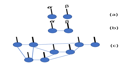
Figure 1: Tensor Network Representing entanglement bonds. (a) represents unentangled state. (b) two entangled qubits, (c) several entangled qubits

Thus Fig. 1 (b) is

$$\bra{\alpha\beta}\ket{\psi}=\sum^{\chi}_{j=1}X^{\alpha}_{j}Y^{\beta}_{j},$$ (1)

here the range of the internal leg is $\chi$, the bond dimension.

In the case that the effects of entangled pairs require a finite time to interact, then one could calculate the time it would take for this information to propagate across a manybody wave function like in Fig. 1 (c). This could be estimated using knowledge of $\chi$ the bond dimension and the total number of bonds.

This leads to the first theorem following from our first postulate:

Theorem 1.

The maximum rate of update for a bulk entangled state is proportional to the total number and dimensions of the bonds as represented by it’s tensor network.

This theorem follows from the fact for the bulk state to evolve into a distinct state different from its current state, it must evolve into one which is orthogonal to it. If the state is not in a distinct state from its current state, then time cannot be said to have advanced for that system. For example if the initial state of our many body entangled wave function is represented by $\psi_{0}$ then for it to update to future time $\psi_{t}$ they must be orthogonal to each other,

$$\bra{\psi_{0}}\ket{\psi_{t}}=0$$ (2)

where

$$\ket{\psi_{t}}=\sum_{n}c_{n}e^{-i\frac{E_{n}t}{\hbar}}\ket{E_{n}}.$$ (3)

Before this process can be complete all information such as a collapse of one member via measurement must have reached all nodes in the tensor network which are connected otherwise unitarity will be violated.

We introduce a $\delta t_{min}$ which represents the minimum number of orthogonal updates in an observing ‘non-entangled’ system compared to the entangled-system. By our conjecture, it is how many time tics in the non-gravitational system necessary to observe one tic in the gravitating system. A consequence of Theorem 1, is that this minimum will grow with the size of the tensor network and number and size of the entangled bonds.

III Relationship between Mass-Energy and Quantum Correlations

It has been proposed that number of entangled chains of particles is proportional to the mass-energy of a given system:

$$N_{E}\propto E.$$ (4)

Here $N_{E}$ represents the number of entangled bonds. This is implied by Lin et al. (2015) which relates energy to the entanglement entropy. It is also the conclusion of Leichenauer et al. (2018) and a consequence of the Quantum Null Energy Condition which relates the stress energy tensor to Von Neuman entropy via:

$$S_{vv}^{\prime\prime}\leq 2\pi\langle T_{vv}\rangle.$$ (5)

Qualitatively it has been shown Linden et al. (2009) that for a physical system the introduction of a new member or particle causes a thermodynamic equilibration process which generates the formation of quantum entanglement with the system. Thus Eq. 4 is justified since each additional particle which becomes locally entangled with a given system and will add another bond in the tensor network for the whole system. It should be obvious that more mass-energy leads to more potential particles from a field-theory point of view and more bonds of entanglement will be created.

Theorem 2.

The total mass-energy of a given system is proportional to the amount of entanglement as represented by the number and dimension of the bonds in a tensor network representation

IV Tunneling time as time dilation?

Calculating $\delta t_{min}$ by counting up all the bonds and their dimensions in a given tensor network is challenging since we do not yet know how to quantify how the time delay scales with each additional bond and its dimension.

A clue to the dependence of the time delay on total mass-energy might be found in the tunneling time experimental and theoretical workCamus et al. (2017), Büttiker (1983), Landsman et al. (2014), Pollak and Miller (1984). Experimental work appears consistent with the theoretical form given by the Feynman Path Integral formulation and Larmor time approach.

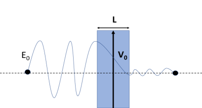
Figure 2: Standard tunneling example through a potential barrier $V_{0}$ of length $L$ and incident particle of mass $m$ and energy $E_{0}$

Both give a functional form for the delay time as:

$$t_{T}=\hbar\frac{\partial\ln|T(E_{o})|}{\partial E_{0}}.$$ (6)

Here $t_{T}$ is the tunneling time and $T(E_{0})$ is the transmission probability for an incident particle of energy $E_{0}$. The functional form of $T(E)$ is given by the nature of the tunneling barrier. The transmission coefficient for crossing a constant potential barrier $V_{0}$, over a distance $L$ is given by (see Fig. 2) :

$$T(E_{0})=e^{-2\sqrt{\frac{2m}{\hbar^{2}}(V_{0}-E_{0})}L}.$$ (7)

Here $m$ is the rest mass of the tunneling particle. Now applying Eq. 6:

$$t_{T} = \frac{\frac{Lm}{\hbar}}{\sqrt{\frac{2m}{\hbar^{2}}(V_{0}-E_{0})}}$$ (8)

$$= \frac{1}{\sqrt{\frac{1}{2L^{2}m}(V_{0}-E_{0})}}.$$

One obtains the time spent under the potential barrier. Since the particle is excluded from existing inside of the barrier, the calculation of tunneling time might be understood as a calculation of the time it takes for quantum state information to propagate through a bulk mass-energy system. This encapsulates the second postulate:

Postulate 2.

The transmission time for quantum information through a bulk mass-energy system is proportional to the quantum tunneling time through the system.

It seems appropriate to guess that information about the update to a particle’s quantum state follows a similar calculation.

Indeed in this form it looks suspiciously similar to the standard time dilation form in the presence of mass-energy. One might imagine time dilation as a result of the time delay for the propagation of quantum state information across a total bulk mass-energy given by $E_{T}$.

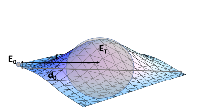
Figure 3: Formulating time dilation as tunneling time. $E_{T}$ is the total mass-energy of the gravitating object (outlined in grey sphere), $r$ the distance to the center of it’s mass, $E_{0}$ the test particle’s mass-energy and $d_{o}$ the distance tunneled (causal distance). The grid is the tensor network or space-time with a bulge representing more network bonds caused by the concentration of mass-energy $E_{T}$.

if we assume the potential which is being tunneled through is a linear function of the total mass-energy of the object $V_{0}=aE_{T}=aMc^{2}$, (see Fig. 3) across a length $L=d_{0}$. Here $a$ is some yet to be determined porpotionality constant. Then by analogy to Eq. 8, we define a transmission coefficient for the state collapse $T_{c}$:

$$T_{c}(E_{0})=e^{-2d_{0}\sqrt{\frac{2m_{0}}{\hbar^{2}}(aMc^{2}-E_{0})}}.$$ (9)

Here $E_{0}$ and $m_{0}$ now represents the kinetic energy and rest mass of test particle approaching an object of potential $aMc^{2}$ respectively. One could interpret $E_{0}$ and $m_{0}$ as the minimal kinetic energy and rest mass of the vacuum.

$d_{0}$ for the cases of calculating transmission coefficients is fixed for a fixed time scale, a sort of minimum distance for a given time duration, beyond which quantum correlation updates are assumed to be unnecessary to preserve unitarity. In some sense the project of building up space-time from entanglement means that ’distances’ between things are given by the level of entanglement of the space around them. So by definition two patches of space at a distance $d$ from each other is more entangled than two patches of space at a distance $2d$ from each other. So for example $d_{0}$ represents some average quantum correlation distance of space, representing the natural fall from maximal entanglement at larger distances. Thus beyond a certain average distance correlations are so minimal that they don’t contain information necessary for updates to preserve unitarity. A good candidate for $d_{0}$ would be the causal light cone since we should not expect effects impacting the rate of time evolution to reach beyond the causal light cone.

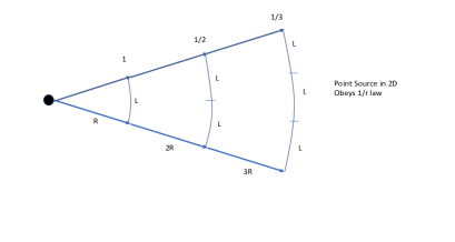
Figure 4: The flux of tensor bonds from a point source will fall off as $\frac{1}{r}$ distance to the source since the flux of entanglement behaves as a two dimensional object.

We further conjecture that the potential $aMc^{2}$ as seen by our test particle, scales with the $1/r$ distance to the center of mass of the object. This is a consequence of Theorem 2 and Postulate 2 and represents our third Theorem:

Theorem 3.

The potential used to calculate the rate of quantum information propagation over the causal distance $d_{0}$ is proportional to $1/r$ distance to the center of mass-energy which generates the potential.

Since by Postulate 2 the tunneling potential used to calculate quantum information propagation is proportional to the mass-energy and by Theorem 2 this same mass-energy is related to the total number of tensor bonds due to entanglement, then the flux of tensor bonds through an space should fall as $1/r$ distance to the center of mass-energy.

The $1/r$ is justified as due to the flux of entanglement experienced by a test particle at a distance $r$ from a source. A three dimensional radiating point source will observe a $1/r^{2}$ flux. However since it has been shown that entanglement obeys an area law, one expects that entanglement flux will behave as a two dimensional object (see Fig. 4). Thus the entanglement flux will follow instead a $1/r$ law. In this case $aMc^{2}$ becomes $b\frac{Mc^{2}}{r}$ with $b$ being an arbitrary proportionality constant having units of length. Now we can write Eq. 8 as:

$$t_{T}=\frac{1}{i\sqrt{\frac{E_{0}}{2d_{0}^{2}m_{0}}(1-\frac{bMc^{2}}{rE_{0}})}}.$$ (10)

If we argue that the kinetic zero point energy is equivalent to zero point mass, $E_{0}=m_{0}c^{2}$ we now obtain:

$$t_{T}=\frac{1}{i\sqrt{\frac{c^{2}}{2d_{0}^{2}}(1-\frac{bMc^{2}}{rE_{0}})}}.$$ (11)

Equating our minimum time update to Eq. 10 via a constant factor $A_{0}$ we obtain:

$$\delta t_{min} = A_{0}t_{T}$$ (12)

$$= \frac{1}{\sqrt{1-\frac{2GM}{rc^{2}}}}.$$

Here $A_{0}=\sqrt{\frac{c^{2}}{2d_{0}^{2}}}$ is a time scale factor which has dropped the complex $i$ since Eq. 6 is properly done using an absolute value. We find that to make $A_{0}=1s^{-1}$ that $c/\sqrt{2}\times seconds=d_{0}=2.11985\times 10^{8}m$. So our intuition that $d_{0}$ is related to the causal light cone appears justified, only it is scaled by $\sqrt{2}$.

Further we have identified $b=\frac{2GE_{0}}{c^{4}}$, with $G$ the gravitational constant. Using this we can derive a relationship for the zero point kinetic energy:

$$E_{0}=\frac{bc^{4}}{2G}$$ (13)

If we pick the Planck length for $b=l_{p}=\sqrt{\frac{\hbar G}{c^{3}}}\approx 1.6\times 10^{-35}$m then we get $E_{0}=9.7\times 10^{8}$ J. If we calculate the energy density by dividing by $l_{p}^{3}$ we get $2.36\times 10^{113}J/m^{3}$. This is almost exactly the high end estimate for vacuum energy density given using Planck’s approach. In pure constants, the vacuum energy density becomes:

$$\rho_{E}=\frac{c^{7}}{2G^{2}\hbar}.$$ (14)

Thus using the tunneling time expression, we have recovered the standard time dilation in a gravitation field:

$$t_{f}=\frac{t_{0}}{\sqrt{1-\frac{2GM}{rc^{2}}}}$$ (15)

Here $t_{f}$ is the is the coordinate time between events for a fast-ticking observer at an arbitrarily large distance from the massive object, $G$ is the Gravitational constant, $M$ is the mass of the object creating the gravitational field and $r$ is the radial coordinate and $t_{0}$ the observed time for the observer.

V Discussion

This attempt to derive the mass-energy time dilation equation using the tunneling time formula from quantum mechanics has the appeal that one can recover a believable quantum correlation distance proportional to the causal light cone. As well as a vacuum energy density consistent with older and higher estimates is also recovered. This might be significant since a large issue in reconciling quantum mechanics with General relativity has been accounting for the large vacuum energy density predicted by quantum mechanics. Here the large energy density follows, as a natural consequence of this derivation.

Starting with the gravitational time dilation equation one should be able to re-derive Einstein’s field equations. Here the governing idea is that mass-energy slows the update of quantum states due to the finite time it takes to update quantum correlations in parallel. It is this differential in time updates which drives the emergence of the force of gravitation.

References

- Camus et al. (2017) N. Camus, E. Yakaboylu, L. Fechner, M. Klaiber, M. Laux, Y. Mi, K. Z. Hatsagortsyan, T. Pfeifer, C. H. Keitel, and R. Moshammer, Phys. Rev. Lett. 119, 023201 (2017).
- Van Raamsdonk (2010) M. Van Raamsdonk, Gen. Rel. Grav. 42, 2323 (2010), [Int. J. Mod. Phys.D19,2429(2010)], arXiv:1005.3035 [hep-th] .
- Ron Cowen (2015) Ron Cowen, “The quantum source of space-time,” NATURE — NEWS FEATURE (2015), https://www.nature.com/news/the-quantum-source-of-space-time-1.18797.
- Maldacena and Susskind (2013) J. Maldacena and L. Susskind, Fortsch. Phys. 61, 781 (2013), arXiv:1306.0533 [hep-th] .
- Jacobson (1995) T. Jacobson, Phys. Rev. Lett. 75, 1260 (1995).
- Lashkari et al. (2014) N. Lashkari, M. B. McDermott, and M. Van Raamsdonk, JHEP 04, 195 (2014), arXiv:1308.3716 [hep-th] .
- Lin et al. (2015) J. Lin, M. Marcolli, H. Ooguri, and B. Stoica, Phys. Rev. Lett. 114, 221601 (2015).
- Verlinde (2017) E. P. Verlinde, SciPost Phys. 2, 016 (2017), arXiv:1611.02269 [hep-th] .
- Bekenstein (1973) J. D. Bekenstein, Phys. Rev. D7, 2333 (1973).
- Margolus and Levitin (1998) N. Margolus and L. B. Levitin, 4th Workshop on Physics and Computation (PhysComp 96) Boston, Massachusetts, November 22-24, 1996, Physica D120, 188 (1998), arXiv:quant-ph/9710043 [quant-ph] .
- Brown et al. (2016) A. R. Brown, D. A. Roberts, L. Susskind, B. Swingle, and Y. Zhao, Phys. Rev. D93, 086006 (2016), arXiv:1512.04993 [hep-th] .
- Moreva et al. (2014) E. Moreva, G. Brida, M. Gramegna, V. Giovannetti, L. Maccone, and M. Genovese, Phys. Rev. A89, 052122 (2014), arXiv:1310.4691 [quant-ph] .
- DeWitt (1967) B. S. DeWitt, Phys. Rev. 160, 1113 (1967).
- Kitada (1994) H. Kitada, Nuovo Cim. B109, 281 (1994), arXiv:astro-ph/9309051 [astro-ph] .
- Dugić and Ćirković (2002) M. Dugić and M. M. Ćirković, Physics Letters A 302, 291 (2002).
- Leichenauer et al. (2018) S. Leichenauer, A. Levine, and A. Shahbazi-Moghaddam, (2018), arXiv:1802.02584 [hep-th] .
- Linden et al. (2009) N. Linden, S. Popescu, A. J. Short, and A. Winter, Phys. Rev. E79, 061103 (2009), arXiv:0812.2385 [quant-ph] .
- Büttiker (1983) M. Büttiker, Phys. Rev. B 27, 6178 (1983).
- Landsman et al. (2014) A. S. Landsman, M. Weger, J. Maurer, R. Boge, A. Ludwig, S. Heuser, C. Cirelli, L. Gallmann, and U. Keller, Optica 1, 343 (2014).
- Pollak and Miller (1984) E. Pollak and W. H. Miller, Phys. Rev. Lett. 53, 115 (1984).