Linear polarization in gamma-ray burst prompt emission

Abstract

Despite being hard to measure, GRB prompt $\gamma$-ray emission polarization is a valuable probe of the dominant emission mechanism and the GRB outflow’s composition and angular structure. During the prompt emission the GRB outflow is ultra-relativistic with Lorentz factors $\Gamma\gg 1$. We describe in detail the linear polarization properties of various emission mechanisms: synchrotron radiation from different magnetic field structures (ordered: toroidal $B_{\rm tor}$ or radial $B_{\parallel}$, and random: normal to the radial direction $B_{\perp}$), Compton drag, and photospheric emission. We calculate the polarization for different GRB jet angular structures (e.g. top-hat, Gaussian, power-law) and viewing angles $\theta_{\rm obs}$. Synchrotron with $B_{\perp}$ can produce large polarizations, up to $25\%\lesssim\Pi\lesssim 45\%$, for a top-hat jet but only for lines of sight just outside ($\theta_{\rm obs}-\theta_{j}\sim 1/\Gamma$) the jet’s sharp edge at $\theta=\theta_{j}$. The same also holds for Compton drag, albeit with a slightly higher overall $\Pi$. Moreover, we demonstrate how $\Gamma$-variations during the GRB or smoother jet edges (on angular scales $\gtrsim 0.5/\Gamma$) would significantly reduce $\Pi$. We construct a semi-analytic model for non-dissipative photospheric emission from structured jets. Such emission can produce up to $\Pi\lesssim 15\%$ with reasonably high fluences, but this requires steep gradients in $\Gamma(\theta)$. A polarization of $50\%\lesssim\Pi\lesssim 65\%$ can robustly be produced only by synchrotron emission from a transverse magnetic field ordered on angles $\gtrsim\!1/\Gamma$ around our line of sight (like a global toroidal field, $B_{\rm tor}$, for $1/\Gamma<\theta_{\rm obs}<\theta_{j}$). Therefore, such a model would be strongly favored even by a single secure measurement within this range. We find that such a model would also be favored if $\Pi\gtrsim 20\%$ is measured in most GRBs within a large enough sample, by deriving the polarization distribution for our different emission and jet models.

1 Introduction

The emission mechanism that produces the soft $\gamma$-ray photons during the exceptionally bright but brief prompt emission phase in gamma-ray bursts (GRBs) is still unclear (see e.g. Kumar & Zhang, 2015, for a review). The non-thermal spectrum of the prompt emission is traditionally fit by the empirical Band-function (Band et al., 1993) that features two power laws that smoothly join at the photon energy $E_{\rm pk}$ where $\nu F_{\nu}$ peaks. A popular model for its origin is optically-thin synchrotron emission from relativistic electrons that are accelerated at internal shocks that form due to the collision of baryonic shells in a matter-dominated outflow with a variable Lorentz factor $\Gamma$ (e.g. Rees & Mészáros, 1994; Papathanassiou & Mészáros, 1996; Sari & Piran, 1997; Daigne & Mochkovitch, 1998). However, this model has been challenged by observations of many GRBs for which synchrotron emission fails (e.g. Crider et al., 1997; Preece et al., 1998, 2002; Ghirlanda, Celotti, Ghisellini, 2003) to produce the correct low-energy spectral slope below $E_{\rm pk}$ (however, see, e.g. Oganesyan et al., 2017; Ravasio et al., 2018, where synchrotron emission has been shown to fit the low energy spectrum with the addition of a spectral break below $E_{\rm pk}$). This inconsistency led to the consideration of alternative models where the main radiation process is multiple inverse-Compton scatterings by sub-relativistic electrons below the Thomson photosphere. Such models also yield a Band-like spectrum and fall under a general class of dissipative photosphere models (see, e.g., Beloborodov & Mészáros 2017 for a review; and see, e.g., Gill & Thompson 2014; Thompson & Gill 2014; Vurm & Beloborodov 2016 for numerical treatments).

The emission mechanism and the magnetic field structure are related to the outflow composition and the dissipation mechanism. In the standard ‘fireball’ scenario (e.g. Rees & Mészáros, 1994) the outflow is launched radiation dominated and optically thick to Thomson scattering ($\tau_{T}>1$) due to the small number (even with a mass as small as $10^{-7}M_{\odot}$) of entrained baryons. Its initial temperature is typically around a few MeV, which results in copious production of $e^{\pm}$-pairs via $\gamma\gamma$-annihilation that further increases $\tau_{T}$. Adiabatic expansion of the flow under its own pressure converts the radiation field energy to kinetic energy of the entrained baryons. This gives rise to a kinetic energy or matter dominated flow, where the energy is released in internal shocks between multiple baryonic shells that form due to variations in $\Gamma$ within the outflow. On the other hand, the outflow can be launched Poynting-flux dominated (e.g. Thompson, 1994; Lyutikov & Blandford, 2003), where the magnetization parameter $\sigma$ (the magnetic to particle energy flux ratio; see Eq. 1) is initially $\sigma_{0}\gg 1$. In this case magnetic reconnection may efficiently dissipate magnetic energy and accelerate particles in magnetically dominated ($\sigma>1$) regions within the outflow, which may power the prompt GRB emission. Such magnetic reconnection requires a flipping of the magnetic field polarity near the central source, which persists out to large distances, such as in a striped wind from a pulsar or magnetar, or by stochastic field flips during accretion onto a black hole.

There are also intermediate scenarios in which the outflow is launched Poynting flux dominated, with $\sigma_{0}\gg 1$ near the central source, but then $\sigma$ gradually decreases with the distance from the source as the outflow is accelerated. Initially acceleration is tied to jet collimation, but in GRBs this typically saturates at $\sigma\gg 1$ and the flow becomes conical. Further acceleration can proceed either through gradual magnetic reconnection in a striped wind over a large range of radii (e.g. Thompson, 1994; Lyubarsky & Kirk, 2001; Spruit et al., 2001; Drenkhahn & Spruit, 2002; Drenkhahn, 2002) or without magnetic dissipation in a strongly variable outflow (Granot, Komissarov & Spitkovsky, 2011). In the latter case kinetic dominance ($\sigma<1$) may be achieved, which allows efficient energy dissipation in internal shocks, even though the outflow was initially magnetically dominated ($\sigma_{0}\gg 1$). All of these scenarios are reasonably plausible and can potentially explain the non-thermal GRB prompt emission spectrum (see e.g. Granot et al., 2015, for a review). However, the magnetic field structure in the emission region may be very different in these two scenarios, as discussed in § 3.1.

Polarization measurements of the prompt emission can shine some much needed light on the important questions regarding the composition of the flow, the magnetic field structure, and the dominant emission mechanism. In particular, they can be useful for determining the dominant prompt emission mechanism, and may help distinguish between different magnetic field structures, which can both help constrain the outflow composition. Furthermore, the degree of polarization critically depends on GRB jet’s angular structure and on our viewing angle $\theta_{\rm obs}$ from its symmetry axis. Therefore, knowledge of the degree of polarization along with the spectral properties of the burst can help distinguish between uniform jets with sharp edges (top-hat jet) and more smoothly varying structured jets.

In this work, we first present a comprehensive overview of the different emission mechanisms that can explain the typical “Band”-like non-thermal prompt emission spectrum, and discuss their expected linear polarization signatures. Reviews on this topic, including theoretical modeling and/or observational results, have been presented, e.g., by Lazzati (2006); Toma et al. (2009); Toma (2013); Covino & Götz (2016). Here, we have endeavoured to present what we consider to be the most plausible emission mechanisms for the prompt GRB: optically-thin synchrotron radiation from both random and ordered magnetic fields, Compton drag, and photospheric emission. Synchrotron self-Compton emission has been considered in the past to explain the prompt emission spectrum, but since it is disfavored by the GRB energetics (see e.g. Piran, Sari, & Zou, 2009) and a featureless high energy spectrum reported by Fermi-LAT, we do not discuss it here. However, the expected polarization from this mechanism is discussed by Chang & Lin (2014).

If the magnetic field coherence length is much smaller than the gyro-radius of particles, then synchrotron radiation, the theory for which is derived for homogeneous magnetic fields, is not the correct description of the radiative mechanism by which relativistic particles cool. In this case, the particles experience small pitch-angle scattering where their motion is deflected by magnetic field inhomogeneities by angles that are smaller than the beaming cone of the emitted radiation ($1/\gamma_{e}$). This scenario of “jitter-radiation” has been proposed as a viable alternative to synchrotron radiation (Medvedev, 2000), where it has been shown to yield harder spectral slopes that cannot be obtained in optically thin synchrotron emission. In addition, this radiation mechanism can produce much sharper spectral break at $E=E_{\rm pk}$, as compared to synchrotron radiation, which agrees better with observations. However, Burgess et al. (2018) claim that GRB spectra obtained by Fermi-GBM are well fit by a synchrotron emission model. The small-scale magnetic fields needed in this scenario are produced in relativistic collisionless shocks via the Weibel instability and the expected polarization if such a field is completely confined to a slab that is normal to the local fluid velocity has been calculated in Mao & Wang 2013; Prosekin et al. 2016; Mao & Wang 2017. There it was shown that the maximum degree of polarization is obtained when the slab is viewed close to edge on. For smaller off-axis viewing angles that can yield measurable fluences in GRBs, jitter-radiation produces almost negligible levels of polarization. For this reason we do not consider this mechanism in this work.

In photospheric emission models, the jet has to be dissipative or heated as it expands from an optically thick to an optically thin state. Without any dissipation the radiation field that decouples from matter at the photospheric radius would have a quasi-thermal spectrum (e.g. Beloborodov, 2010), where the spectrum below the peak energy $E_{\rm pk}$ would be much harder than generally observed. Comptonization of softer photons below the photosphere has been shown to yield a spectrum that is softer than blackbody and better agrees with observations (e.g. Beloborodov, 2010; Vurm, Lyubarsky, & Piran, 2013; Thompson & Gill, 2014). Continued heating as the jet becomes optically thin (e.g. Giannios, 2008; Vurm & Beloborodov, 2016) or even radially localized heating outside of the photosphere (Gill & Thompson, 2014) can give rise to the non-thermal spectrum above the peak energy. Since the peak and the higher energy spectrum forms through multiple Compton scattering, the polarization degree of the radiation field is washed away as there is no particular direction for the electric field vector. If the flow is uniform then almost negligible polarization remains when averaged over the entire GRB image. This symmetry can be broken in two ways. First, it has been shown, and discussed later in this work as well, that if the flow has a steep gradient in the LF angular profile, polarization degree of up to $\Pi\sim 20\%$ can be observed (Lundman, Pe’er, & Ryde, 2014). Second, if the low energy spectrum at $E\ll E_{\rm pk}$ arises due to synchrotron emission near the photosphere (Lundman, Vurm, & Beloborodov, 2018), then the local magnetic field would impart a particular direction with which the electric field vector would be aligned, resulting in polarized emission. To carry out a self-consistent treatment of polarized emission in a dissipative photospheric model is outside the scope of this work, and therefore only the non-dissipative photospheric model is discussed here.

After deriving the level of linear polarization expected from different radiative processes, outflow geometries and viewing angles, we perform a statistical analysis of the expected level of polarization for these different scenarios by simulating a sample of $10^{4}$ GRBs. This analysis is carried out using simple Monte Carlo (MC) simulations, where the underlying assumption is that due to low photon statistics a statistically significant measurement of polarization generally entails, in addition to an overall high fluence, integration over multiple pulses in a given emission episode. These pulses can arise from, e.g., multiple internal shocks between distinct shells launched intermittently by the central engine, or different magnetic reconnection sites corresponding to different magnetic field polarity flips at different radial locations within the outflow. In both cases $\Gamma$ is expected to vary between different pulses (typically by $\Delta\Gamma\sim\Gamma$), which affects the degree of polarization obtained from integrating over multiple pulses. A similar effect may be caused by a gradual growth in the jet half-opening angle $\theta_{j}$ throughout the course of the GRB (while $\Delta\theta_{j}\sim\theta_{j}$ may be expected, even $\Delta\theta_{j}\gtrsim 1/\Gamma$ could have a large effect on the observed polarization).

Furthermore, different GRBs are observed from different viewing angles $\theta_{\rm obs}$, and a spread in $\theta_{\rm obs}$ will yield different levels of polarization in a given sample of GRBs. This effect is intricately linked with the geometry of the outflow, where the degree of polarization changes significantly between a top-hat jet and structured jet. In addition, $\theta_{\rm obs}$ and the jet angular structure also affect the measured fluence, which significantly drops at large off-axis $\theta_{\rm obs}$. This effect is much more pronounced for a top-hat jet as compared to a structured jet. The relative contribution of each pulse scales with its number of detected photons (or more precisely the number of Compton events that can be used to measure the polarization). The MC simulations conducted in this work take into account the drop in fluence for larger viewing angles by considering a distribution of fluence weighted viewing angles for a fixed jet half-opening (core) angle in the case of a top-hat (structured) jet. In addition, it accounts for the variation in $\Gamma$ when integrating over multiple pulses.

Throughout this work, we consider an axi-symmetric relativistic outflow launched by a central engine (a black hole or a rapidly spining magnetar) in the coasting phase, with a bulk LF $\Gamma=(1-\beta^{2})^{-1/2}\gg 1$ that corresponds to the dimensionless fluid velocity $\vec{\beta}=\vec{v}/c$, where $c$ is the speed of light. Each pulse is assumed to originate from a single thin shell (of radial width $\Delta\ll R/\Gamma^{2}$) with some $\Gamma(\theta)$ distribution, where $\Gamma$ may vary between different pulses according to some probability distribution. For simplicity we consider only radially expanding outflows, such that $\hat{\beta}=\hat{r}$. We consider both top-hat jets and structured jets, where in the former case, the outflow has an angular size with $10\lesssim\xi_{j}\equiv(\Gamma\theta_{j})^{2}\lesssim 10^{3}$, where $\theta_{j}$ is the half-opening angle of the jet. Angles measured with respect to the LOS are shown with a tilde, e.g. the polar angle measured from the LOS is $\tilde{\theta}$. For a top-hat jet, the emission is assumed to drop rapidly for $\theta>\theta_{j}$, effectively giving the outflow a sharp edge. When the outflow has an angular structure, the total energy is dominated by the core with $\xi_{c}\equiv(\Gamma_{c}\theta_{c})^{2}$ where $\theta_{c}$ and $\Gamma_{c}$ are respectively the angular size and LF of the core that is surrounded by low energy material extending to larger polar angles $\theta$. Outside the core the LF also drops according to the given prescription, however, all results pertaining to the structured jet case make sure that even at large $\theta$ the LF of the material is $\Gamma\gtrsim 10$. Therefore, all results in this work are obtained for an ultra-relativistic flow.

The outline of the paper is as follows. In §2, we give a brief overview of the measurements of linear polarization obtained during the prompt phase as well as from early afterglow emission. We start by discussing the origin of polarization from synchrotron emission in §3. The likely origin and configuration of the magnetic field in the outflow is discussed in §3.1. In §3.2, we provide a general treatment for calculating the degree of polarization averaged over the entire GRB image. This formalism also applies to all other emission mechanisms discussed in this work. In a spherical flow, polarization arising from a random magnetic field configuration that lies entirely in the plane of the ejecta averages to zero. Therefore, effects due to the angular structure of the jet and the observer’s viewing angle become important in yielding non-vanishing degree of polarization. We first present the general equations for the polarization treatment that apply to off-axis observers and different magnetic field configurations in §3.3. Polarized emission from on-axis top-hat jets from an ordered magnetic field is treated in §3.4 along with the temporal evolution of the degree of polarization over a single pulse. Off-axis top-hat jets with ordered and random magnetic fields are discussed in §3.5. A serious issue for off-axis top-hat jets is the rapid drop in fluence (§3.6) for viewing angles larger than the jet opening angle. This effect is important when modeling GRB polarization since all detectors are flux-limited and only detect emission from regions of the flow brighter than the detector threshold. The top-hat jet model, although simple yet instructive, is an idealization and may not be the true description of the structure of relativistic GRB jets. Instead, the jet may manifest angular structure and the emission may drop rather gradually outside of a compact core. We discuss polarization from structured jets in §3.7. Alternative radiative mechanisms that can explain the non-thermal spectra of GRBs and also yield polarized emission are treated next. In §4, we first present the general formalism that describes the mechanism of Compton drag (§4.1), where relativistically hot electrons inverse Compton scatter ambient radiation fields. Later, we specialize to the case of cold electrons in a relativistic outflow (§4.2) and show the degree of polarization for off-axis top-hat jets. In §5, we first discuss the radiation transfer of polarized emission in a matter-dominated non-dissipative fireball. However, after averaging over the GRB image a spherically symmetric outflow would yield vanishing polarization. Analytic treatment of polarized photospheric emission, based on the radiation transfer solution, from a structured jet is presented for the first time in this work (§5.1). In general, the GRB prompt emission suffers from low photon statistics at high energies. This becomes an even more of an issue for polarization measurements. Unless the burst is exceptionally bright, one is forced to integrate over multiple pulses to obtain statistically significant results. We treat this topic and its effect on the net polarization due to varying $\Gamma$ between pulses in §6. After having discussed the predictions for the degree of polarization arising in synchrotron emission for different viewing geometries and jet structures, we carry out a MC simulation of $10^{4}$ GRBs in §7 to determine the most likely magnetic field configuration for a given measurement of linear polarization. In order to yield a robust result, we take into account the effects of different $\theta_{\rm obs}$ in different GRBs and integration over multiple pulses within a single GRB with fixed $q=\theta_{\rm obs}/\theta_{j}$ but varying $\Gamma$. Finally, in §8 we discuss salient points of this work and present important implications of the results.

GRB	$\Pi$ (%)	PA (∘)	$\sigma_{\rm det}~{}(\Pi>0\%)$	Instrument	Ref.
021206	$80\pm 20$	–	$>\!5.7$	RHESSId	Coburn & Boggs (2003)
	$0$		–		Rutledge & Fox (2004)
	$41^{+57}_{-44}$		–		Wigger et al. (2004)
041219A	$98\pm 33$		$\sim\!2.3$	INTEGRAL-SPIe	Kalemci et al. (2007)
	$63^{+31a}_{-30}$	$70^{+14}_{-11}$	$\sim\!2$		McGlynn et al. (2007)
	$43\pm 25^{b}$	$38\pm 16$	$<\!2$	INTEGRAL-IBIS	Götz et al. (2009)
061122	$>\!33$ ($90\%$ CL)	$160\pm 20$	–	INTEGRAL-IBIS	Götz et al. (2013)
100826Ac	$27\pm 11$	–	$2.9$	IKAROS-GAP	Yonetoku et al. (2011b)
100826Ap1c	$25\pm 15$	$159\pm 18$	$2.0$
100826Ap2c	$31\pm 21$	$75\pm 20$	$1.6$
110301A	$70\pm 22$	$73\pm 11$	$3.7$	IKAROS-GAP	Yonetoku et al. (2012)
110721A	$84_{-28}^{+16}$	$160\pm 11$	$3.3$	IKAROS-GAP	Yonetoku et al. (2012)
140206A	$>\!28$ ($90\%$ CL)	$80\pm 15$	–	INTEGRAL-IBIS	Götz et al. (2014)
151006A	$<\!84$	$-$	$-$	AstroSat-CZTI	Chattopadhyay et al. (2017)
160106A	$69\pm 24$	$-23\pm 12$	$\gtrsim\!3$	AstroSat-CZTI	Chattopadhyay et al. (2017)
160131A	$94\pm 33$	$41\pm 5$	$\gtrsim\!3$	AstroSat-CZTI	Chattopadhyay et al. (2017)
160325A	$59\pm 28$	$11\pm 17$	$\sim\!2.2$	AstroSat-CZTI	Chattopadhyay et al. (2017)
160509A	$<\!92$	$-$	$-$	AstroSat-CZTI	Chattopadhyay et al. (2017)
160530A	$<\!46$ ($90\%$ CL)	–	–	COSIg	Lowell et al. (2017)
160607A	$<\!77$	$-$	$-$	AstroSat-CZTI	Chattopadhyay et al. (2017)
160623A	$<\!46$	$-$	$-$	AstroSat-CZTI	Chattopadhyay et al. (2017)
160703A	$<\!55$	$-$	$-$	AstroSat-CZTI	Chattopadhyay et al. (2017)
160802A	$85\pm 30$	$-36\pm 5$	$\gtrsim\!3$	AstroSat-CZTI	Chattopadhyay et al. (2017); Chand et al. (2018a)
160821A	$54\pm 16$	$-39\pm 4$	$\gtrsim\!3$	AstroSat-CZTI	Chattopadhyay et al. (2017)
160821Ah	$66^{+26}_{-27}$		$\sim\!5.3$	AstroSat-CZTI	Sharma et al. (2019)
160821Ap1h	$71^{+29}_{-41}$	$110^{+14}_{-15}$	$3.5$	AstroSat-CZTI
160821Ap2h	$58^{+29}_{-30}$	$31^{+12}_{-10}$	$4$	AstroSat-CZTI
160821Ap3h	$61^{+39}_{-46}$	$110^{+25}_{-26}$	$3.1$	AstroSat-CZTI
160910A	$94\pm 32$	$44\pm 4$	$\gtrsim\!3$	AstroSat-CZTI	Chattopadhyay et al. (2017)
161218A	$9$	40	$\sim\!1.7$	POLAR	Zhang et al. (2019)
	$<\!41$ ($99\%$ CL)	–	–
170101A	$8$	164	$\sim\!1.5$	POLAR	Zhang et al. (2019)
	$<\!30$ ($99\%$ CL)	–	–
170114A	$4$	164	$\sim\!1.5$	POLAR	Zhang et al. (2019); Burgess et al. (2019)
	$<\!28$ ($99\%$ CL)	–	–
170114Ap1f	$15$	122	$\sim\!1.8$
170114Ap2f	$41$	17	$\sim\!2.8$
170127C	$11$	38	$\sim\!1.9$	POLAR	Zhang et al. (2019)
	$<\!68$ ($99\%$ CL)	–	–
170206A	$10$	106	$\sim\!1.5$	POLAR	Zhang et al. (2019)
170206A	$<\!31$ ($99\%$ CL)	–	–
171010A	$\sim\!40$	variable	–	AstroSat-CZTI	Chand et al. (2018b)

Table 1: Measured degree of linear polarization and position angle in the prompt phase of GRBs. The detection significance $\sigma_{\rm det}$ is the significance of measuring $\Pi>0\%$. The quoted errors are at the $1\sigma$ level. ^aMeasured for the brightest pulse of duration 66 s. ^b Measured for the second peak lasting $40\,$s. ^cThe main prompt emission is divided into two time intervals, p1 featuring a 47 s broad flare (line 1), and 53 s long p2 consisting of multiple pulses (line 3). Line 1 jointly fits p1 and p2 assuming they have the same $\Pi$ but allowing and indeed finding a different PA between them. ^dReuven Ramaty High Energy Solar Spectroscopic Imager. ^eInternational Gamma-Ray Astrophysics Laboratory. ${}^{f}\Pi$ obtained for two equal 2 s time bins within a single pulse, with a significant change in PA between them. ^gCompton Spectrometer and Imager. ^hAverage polarization over the single emission episode, with a Fermi-GBM (AstroSat-CZTI) $T_{90}=43\,$s ($42\,$s), that showed variable polarization levels and PA during three distinct time intervals p1, p2, p3 within the emission episode.

2 Observations

2.1 Measured degree of polarization of prompt emission

To robustly measure a significantly high degree of polarization, a high signal-to-noise ratio is needed. Due to the dearth of photons during the prompt phase, this becomes a serious issue. Therefore, reports of linear polarization thus far have at best been able to establish a $\sim 3\sigma$ detection significance (however, see e.g. Sharma et al. 2019), and even that only in a handful of cases. The first detection of linear polarization during the prompt phase was reported by Coburn & Boggs (2003) for GRB 021206, where they reported a high degree of polarization (see Table 1). This result was later refuted by Rutledge & Fox (2004) and Wigger et al. (2004), who found no significant degree of polarization. Another controversial result was reported for GRB 041219 (Kalemci et al., 2007; McGlynn et al., 2007), but the low ($\sim 2\sigma$) statistical significance of the result did not lead to any strong conclusions. Few upper and lower limits, albeit only at the $90\%$ confidence level, have been reported using the INTEGRAL-IBIS and COSI data.

More robust measurements of linear polarization came from the “GAmma-ray bursts Polarimeter” (GAP) on board the “Interplanetary Kite-craft Accelerated by the Radiation Of the Sun” (IKAROS) spacecraft (Yonetoku et al., 2011a). The GAP measured modest to high degree of polarization for three GRBs (Yonetoku et al., 2011b, 2012). Further measurements of linear polarization at a detection significance of $\gtrsim 2.5\sigma$, with some at a lower significance, have come from the CZTI detector on board AstroSat (Singh et al., 2014). Upper limits on linear polarization for five GRBs with $99\%$ confidence were reported by POLAR, a dedicated GRB polarization detection experiment onboard China’s Tiangong-2 space laboratory (Zhang et al., 2019). Under the assumption that all five GRBs are indeed polarized, a joint analyses revealed an average degree of polarization of $\langle\Pi\rangle=10\%$ with a $0.1\%$ probability that all five sources have either $\Pi<5\%$ or $\Pi>16\%$.

2.2 Change in polarization angle

Thus far, most measurements of linear polarization during the prompt phase have been reported with a fixed polarization angle (PA), and in only four cases a change in PA has been reported. In GRB 100826A, a change in PA was detected between two time intervals corresponding to bright emission episodes with a $3.5\sigma$ confidence level (Yonetoku et al., 2011b), based on a joint fit of the two intervals assuming they had the same $\Pi$ (finding $\Pi>0$ with a significance of $2.9\sigma$). However, when performing separate fits on these two time intervals their individual polarization detection significance is lower ($2.0\sigma$ and $1.6\sigma$; see Table 1). A time-resolved analysis of GRB 170114A, which showed only a single pulse, revealed a large change in the PA between two $2\,$s time bins (Zhang et al., 2019), where the polarization detection significance in each time bin is moderate ($\sim\,$1.8$\sigma$ and $\sim\,$2.8$\sigma$; see Table 1). Burgess et al. (2019) carried out a detailed spectro-polarimetric analysis of this GRB and reached similar conclusions. A large change in the PA was found in the time-resolved analysis of GRB 171010A over three time bins (Chand et al., 2018b), but with a low statistical significance. Finally, Sharma et al. (2019) found variable degree of polarization in a time-resolved analysis of a single emission episode from GRB 160821A, which they divided into three distinct time intervals. Over these intervals the burst emission gradually rises to the peak and then declines and the PA between the three intervals shifts by $\Delta\theta_{p,12}=81^{\circ}\pm 13^{\circ}$ and $\Delta\theta_{p,23}=80^{\circ}\pm 19^{\circ}$ with a fairly high significance of $\sim\!3.5\sigma$ and $\sim\!3.1\sigma$, respectively.

Generally, a time-resolved analysis is not possible due to small number of detected photons. This is further made challenging by the fact that it is actually the Compton events due to scattering in the detector that are used to measure polarization, and they constitute only a fraction of the total number of photons detected from the source. Therefore, to increase the sensitivity of the detection an average polarization as well as an average PA rather than a time-resolved one is generally obtained. However, in bright bursts with multiple pulses, tracking the evolution of the PA can provide critical information that can be used to further constrain the outflow geometry and viewing angle. As we discuss below, in the case of a top-hat jet if the viewing angle is very close to the edge of the jet, $\theta_{\rm obs}\approx\theta_{j}$, then change in $\Gamma$ between distinct pulses will change $\xi_{j}$ which can lead to a change in the PA by $90^{\circ}$. However, this only occurs in this special circumstance, and therefore, a change in PA between different pulses should not be so commonly observed. Alternatively, Deng et al. (2016) have shown, using 3D relativistic MHD simulations and a 3D multi-zone polarization-dependent radiation transfer code, that in the ICMART model (Zhang & Yan, 2011) a $90^{\circ}$ change in the PA can arise due to magnetic reconnection where the local magnetic field orientation, which is orthogonal to the wave vector of the emitted photon, itself switches by $90^{\circ}$ as the field lines are destroyed and reconnected in the emission region.

On the other hand, a change in the PA by an angle $\Delta\theta_{p}$ that is clearly not $0^{\circ}$ or $90^{\circ}$, e.g. $\Delta\theta_{p}\sim 45^{\circ}$, would be challenging to explain by the different emission models presented in this work. Any changes in the geometry or $\Gamma$ of the outflow cannot explain it, as long as the flow remains axi-symmetric with a symmetry axis that does not move during the GRB. The PA evolution is sensitive to changes in the local magnetic field direction within the visible region, and a gradual continuous change in $\theta_{p}$ could potentially arise from a similar change in the direction of the ordered magnetic field in the visible region, though the cause for such a change during the prompt emission is not very clear. An alternative that is worth mentioning is if each pulse is associated with a different “mini-jet” within the outflow (e.g. Lyutikov & Blandford, 2003; Narayan & Kumar, 2009; Kumar & Narayan, 2009; Lazar et al., 2009; Zhang & Yan, 2011), e.g. in the context of stochastic magnetic reconnection events, then this would indeed produce significant deviation from axi-symmetry of the emission regions, and could produce different and mutually randomly oriented PA’s in different pulses, leading to a total polarization that largely follows Eq. (95). This is analogous to the suggested random afterglow polarization variations that may accompany variability in the afterglow lightcurve, which may be induced by a “patchy shell” model for the GRB outflow (Granot & Königl, 2003; Nakar & Oren, 2004) or by a clumpy external medium (Granot & Königl, 2003).

An alternative explanation for a change of $\Delta\theta_{p}\sim 45^{\circ}$ in the PA that appears in Granot & Königl (2003), in which the flow remains axi-symmetric, is a combination of an ordered + random field. In this case the ordered field orientation is assumed to remain fixed, but the relative strength of the random (in 2D) and ordered fields changes during the GRB. In that work it was discussed mainly in the context of afterglows, but the physics is practically the same. One possible difference is the motivation for ordered and random field components. For the afterglow Granot & Königl (2003) envision an ordered field component to arise from shock compression of an ordered field in the external medium, while a random component may be produced at the shock, so that the two components are co-spatial. In the prompt emission a similar picture may arise in which an ordered upstream field may naturally be advected from near the central source, while the random field may either be shock-produced and co-spatial, or alternatively generated at a thin reconnection layer and be confined to its vicinity so that it would not occupy the same region as the ordered field in the bulk of the outflow.

2.3 Early afterglow polarization measurements

Another way of probing the magnetization of the GRB outflow and the magnetic field structure is by obtaining polarization measurements of the early afterglow. As the relativistic ejecta slows down by sweeping up interstellar medium, a reverse shock propagates into it. As a result, shock heated electrons in the ejecta radiate synchrotron photons, the flux of which peaks in the optical at timescales of tens of seconds, which could give rise to the so called “optical flash” lasting for about 10 minutes after the prompt GRB. In most cases, it is not detected at all and its duration can also vary. After the reverse shock has fully crossed the ejecta, the shocked electrons cool adiabatically while the peak of their emission moves to lower frequencies, where it powers a “radio flare” after about 1 day.

Measurements of linear polarization up to few tens of percent have been obtained from the early optical afterglow emission of several GRBs. Most notable examples are: GRB 090102 with $\Pi=(10.2\pm 1.3)\%$ (Steele et al., 2009); GRB 120308A with $\Pi=(28\pm 4)\%$ with a gradual decay over the next ten minutes to $\Pi=16_{-4}^{+5}\%$ (Mundell et al., 2013). Recently, radio/millimeter afterglow observations of GRB 190114C, dominated by the reverse shock component at $t_{\rm obs}\approx 2.2-5.2\,$ hrs, revealed the temporal evolution in the linear polarization from $\Pi=(0.87\pm 0.13)\%$ to $\Pi=(0.60\pm 0.19)\%$ (Laskar et al., 2019). In other cases, radio flares have only yielded low upper limits, e.g. a strict $3\sigma$ upper limit of $\Pi<7\%$ in GRB 991216 (Granot & Taylor, 2005). Both of these observations, and in particular the measurement of gradual rotation of the PA during the observation in GRB 190114C, challenge the model where the outflow is permeated by a large scale ordered toroidal magnetic field.

3 Synchrotron Emission

Relativistic electrons (or $e^{\pm}$-pairs) gyrating in a magnetic field cool by emitting synchrotron photons. In general, synchrotron emission is partially linearly polarized, where the degree of polarization depends critically on the structure of the magnetic field and the observer’s LOS. It is simpler to first examine the polarization arising in the comoving frame from an infinitesimally small region (a fluid element) of the outflow. This will allow us to prescribe a particular magnetic field configuration to that region and calculate the local polarization vector from a given fluid element. The same can then be obtained in the observer’s frame, i.e. on the plane of the sky, through the appropriate Lorentz transformation. Since at high energies (e.g. X-rays, $\gamma$-rays) both the prompt and the afterglow emission regions remain unresolved, to obtain the total degree of polarization one must sum or integrate over the entire GRB image, which receives flux from all of the different fluid elements in the outflow. Before we provide a general prescription for calculating the degree of polarization arising in synchrotron emission, we first give a brief overview of the different magnetic field geometries that have been considered in GRB outflows.

3.1 Likely origin and configuration of the magnetic field

The origin of the magnetic field in relativistic outflows that power GRBs is still a matter of active research and debate. Polarization measurements can help to elucidate its structure, however, so far they have not yielded any conclusive results due to the low statistical significance of the measurements (however, see e.g. Sharma et al. 2019). The magnetic field configuration within the outflow is expected to be affected by its degree of magnetization (the magnetic to particle energy flux ratio),

$$\sigma\equiv\frac{w_{B}^{\prime}}{w_{m}^{\prime}}=\frac{B^{\prime 2}}{4\pi[\rho^{\prime}c^{2}+\hat{\gamma}(\hat{\gamma}-1)^{-1}P^{\prime}]}\xrightarrow[\rm cold]{}\frac{B^{\prime 2}}{4\pi\rho^{\prime}c^{2}}~{},$$ (1)

where $w_{B}^{\prime}$ and $w_{m}^{\prime}$ are the comoving magnetic field and matter enthalpy densities, respectively, $B^{\prime}$ is the comoving magnetic field strength, $\rho^{\prime}$ is the matter rest mass density, $P^{\prime}$ is its pressure, and $\hat{\gamma}$ is the adiabatic index. If the flow is cold, then the matter enthalpy density is simply its rest mass energy density with no pressure term.

The fireball model does not have a clear prediction for the magnetic field structure in the emission region. During the acceleration phase ($R_{0}<R<R_{s}=\eta R_{0}$ where $\eta$ is the energy per unit rest energy and hence the coasting Lorentz factor, and $\Gamma(R_{0})\approx 1$) $\sigma\approx\sigma_{0}<1$ remains unchanged. The same also holds during the coasting phase until the shells, of initial radial width $\Delta_{0}\approx ct_{\varv}$ where $t_{\varv}$ is the source variability time, start to significantly spread radially at $R_{\Delta}\sim\Gamma^{2}(R_{\Delta})\Delta_{0}\sim\eta^{2}\Delta_{0}$. However, $R_{\Delta}$ is also the radius where internal shocks are expected to occur, so in this scenario $\sigma\sim\sigma_{0}<1$ also in the emission region (if it is indeed produced by internal shocks). During the coasting phase the lateral linear size of each fluid element scales as $R$ while its radial size remains constant, so that flux freezing implies $B_{r}\propto R^{-2}$ while $B_{\theta,\phi}\propto R^{-1}$ so that $B_{r}/B_{\theta,\phi}$ decreases by a factor of $R_{\Delta}/R_{s}=\eta ct_{\varv}/R_{0}\gg 1$ and the transverse field components strongly dominate over the radial component. For $10^{-3}\lesssim\sigma\sim\sigma_{0}<1$ the upstream magnetic field is large enough to form the shock transition without the need for significant magnetic field amplification beyond the usual shock compression (e.g. Sironi & Spitkovsky, 2011), so that an ordered upstream field advected from the central source is expected to dominate in the downstream emission region, though in this regime it appears to be difficult to accelerate electrons to a non-thermal energy distribution. For $\sigma<10^{-3}$ shock generated fields via the Weibel instability (which are random and lie predominantly in the plane transverse to the shock normal) dominate over the shock compressed upstream field just behind the shock, and non-thermal electron acceleration becomes efficient.

For outflows that are initially Poynting flux dominated the magnetic field is expected to be ordered on large scales as it is dynamically dominant, and tangled field features within causally connected regions would tend to either straighten out or at least partly reconnect, both leading to much more ordered field configurations. However, magnetic reconnection can tangle the field near the reconnection layer, so that the electrons that are accelerated there may radiate some or even most of their energy in a rather random field before reaching the ordered field in the bulk of the outflow. If kinetic energy dominance ($\sigma<1$) is reached leading to efficient dissipation in internal shocks, this reverts to the discussion above with the addition that in this case the upstream field is expected to be both transverse and ordered on large scales (angles $\gtrsim 1/\Gamma$).

When $\sigma<1$, magnetic fields are dynamically subdominant and plasma motions largely dictate the magnetic field structure. As a result, the magnetic field can be tangled on small scales ($\theta_{B}\ll\theta_{j}$) in the plane normal to the radial direction. In hydrodynamic flows, energy radiated during the prompt emission is expected to be dissipated mainly in internal shocks, where in the emission region near-equipartition magnetic fields are typically assumed to originate via the relativistic two-stream instability (Medvedev & Loeb, 1999). The fields are generated at the relativistic ion-skin depth scales $c\bar{\gamma}_{p}^{1/2}/\omega_{p,i}^{\prime}\sim 10^{3}$ cm, where $\omega_{p,i}^{\prime}$ is the fluid-frame ion plasma frequency and $\bar{\gamma}_{p}$ is the mean thermal energy per unit rest mass energy of protons. The configuration of the field is random within the plane of the shock, and the field strength quickly grows with an e-folding time of $\sim 10^{-7}$ s to near-equipartition level. Still, the field coherence length remains much smaller than the outflow’s angular transverse size as well as its transverse causally connected size, such that $\theta_{B}\ll 1/\Gamma\lesssim\theta_{j}$.

Alternatively, if the flow is launched Poynting-flux dominated, for which $\sigma\gg 1$, the magnetic field is dynamically dominant. In this case, an ordered magnetic field with a large coherence length $1/\Gamma\lesssim\theta_{B}\lesssim\theta_{j}$ can be expected within the relativistic outflow (Lyutikov & Blandford, 2003). For an axially symmetric field configuration, the poloidal component of the magnetic field ($B_{p}\propto r^{-2}$) drops rapidly with radius. Therefore, the toroidal component ($B_{\phi}\propto r^{-1}$) remains dominant at large distances from the central source.

In the following, we consider three magnetic field configurations: (i) a locally ordered field ($B_{\rm ord}$) that is coherent on angular scales $1\lesssim\Gamma\theta\lesssim 10$ and lies entirely in the direction transverse to the local fluid velocity $\vec{\beta}=\vec{\varv}/c$, the direction of which is identified with the local shock normal and radial unit vector with $\hat{\beta}=\hat{r}=\hat{x}\sin\theta\cos\varphi+\hat{y}\sin\theta\sin\varphi+\hat{z}\cos\theta$. We parameterize its direction $\hat{B}_{\rm ord}$ such that its projection onto the $x$-$y$ plane (normal to the jet’s symmetry axis) is $\hat{B}_{0}=\hat{x}\cos\varphi_{B}+\hat{y}\sin\varphi_{B}$. (ii) a tangled magnetic field with components both parallel ($B_{\parallel}$) and perpendicular ($B_{\perp}$) to $\vec{\beta}$. In this case, it is convenient to parameterize the field anisotropy by taking the ratio of the average energy density of the two field components, such that

$$b\equiv\frac{2\langle B_{\parallel}^{2}\rangle}{\langle B_{\perp}^{2}\rangle}~{}.$$ (2)

When $b=0$, the configuration of the magnetic field is that of a completely tangled or random magnetic field ($B_{\perp}$) in the plane normal to the local fluid velocity which is in the radial direction here. On the other hand, when $b\to\infty$ the configuration of the field is that of an ordered field ($B_{\parallel}$) entirely confined in the direction parallel to the local fluid velocity; and finally (iii) a toroidal field ($B_{\rm tor}$) that is ordered in the transverse direction and is axisymmetric with respect to the jet symmetry axis, such that $\hat{B}_{\rm tor}=\hat{\varphi}=-\hat{x}\sin\varphi+\hat{y}\cos\varphi$.

Afterglow polarization measurements after about several hours to a few days typically give fairly low level polarization detections or upper limits of $\Pi\lesssim 1\%-3\%$ (e.g. Covino et al., 2003). This is typically near the jet break time in the afterglow lightcurve, while GRB jet models with a shock generated field can produce $\Pi\sim 10\%-20\%$ near the jet break time. This apparent discrepancy already tentatively suggest that $b$ may not be very far from unity, $0.5\lesssim b\lesssim 2$, in order to suppress the afterglow polarization.

However, the recent short GRB170817A associated with the NS-NS merger gravitational wave event GW170817 provides stricter and more robust constraints on the value of $b$. Detailed theoretical modeling (Gill & Granot, 2018) together with the very elaborate afterglow observations from this event, and in particular the detection of super-luminal motion of the radio flux centroid with an apparent velocity of $\beta_{\rm app}=4.1\pm 0.5$ (Mooley et al., 2018), clearly imply that the late time afterglow emission arises primarily from near the energetic narrow core of a relativistic jet viewed from well outside of its core. The jet structure and viewing angle implied by these observations result in clear predictions for the afterglow linear polarization (Gill & Granot, 2018). A later upper limit on the radio ($2.8\;$GHz) linear polarization of $\Pi<12\%$ (with 99% confitence) at $t=244\;$days (Corsi et al., 2018) is very constraining for the value of $b$, and we find that it robustly implies $0.66\lesssim b\lesssim 1.49$ (Gill & Granot, 2019). It is important to keep in mind that this applies to the effective value of $b$ in the afterglow shock. However, the latter comes from all of the shocked external medium behind the afterglow shock, which experiences significant shear in the radial direction (e.g. Granot, Piran, & Sari, 1999a, b), i.e. each fluid element is stretched more in the radial direction than in the two transverse directions, as it is advected further downstream from the shock. Therefore, the shock produced magnetic field could perhaps be predominantly in the plane of the shock ($b\ll 1$) just behind the shock transition, but become more isotropic ($b\sim 1$) in the bulk of the emitting region due to this significant radial shear (which causes $b$ to increase with the distance behind the shock). This effect and its possible implications are explored in more detail in Gill & Granot (2019). Such a strong radial shear is not expected in internal shocks, so that there the effective value of $b$ may potentially be different (and likely lower, $b<1$) than during the afterglow.

3.2 Observed polarization - general treatment

The degree of polarization for the three magnetic field configurations considered in this work has been calculated in detail in many works (e.g. Ghisellini & Lazzati (1999); Sari (1999); Gruzinov (1999); Granot & Königl (2003); Granot (2003); Lyutikov, Pariev, & Blandford (2003); Granot (2005); Granot & Taylor (2005); see Nava, Nakar, & Piran (2016) for circular polarization). In the following we summarize the important results (see Toma et al., 2009; Toma, 2013, for a review).

The state of polarization of a radiation field that emanates from a given fluid element is most conveniently expressed in terms of the Stokes parameters $I$, $Q$, $U$, $V$. We are interested here in linear polarization for which $V=0$. Here $I$ is the total intensity and the local degree of linear polarization is given by

$$\Pi^{\prime}=\frac{\sqrt{Q^{2}+U^{2}}}{I}~{},$$ (3)

where

$$\frac{U}{I}=\Pi^{\prime}\sin 2\theta_{p}~{},\quad\frac{Q}{I}=\Pi^{\prime}\cos 2\theta_{p}~{},\quad\theta_{p}=\frac{1}{2}\arctan\left(\frac{U}{Q}\right)~{},$$ (4)

with $\theta_{p}$ as the polarization position angle (PA). The Stokes parameters and PA undergo a Lorentz transformation from the comoving to the observer’s frame, whereas the local degree of polarization is a Lorentz invariant (being the ratio of Stokes parameters that undergo the same Lorentz transformation). In what follows, we distinguish between the local degree of polarization $\Pi^{\prime}$ and the global polarization $\Pi$, which is obtained after integrating over the whole GRB image on the plane of the sky as described below.

At any given observer time $t_{\rm obs}$, the observer sees radiation emitted at different lab-frame times $t$ from different fluid elements with lab-frame coordinates ($r$, $\theta$, $\varphi$), where $r$ is the radial distance measured from the central engine, $\theta$ is the polar angle measured from the jet-axis, and $\varphi$ is the azimuthal angle. Here and what follows we use two different coordinate systems, as shown in Fig. 1. The first coordinate system $(x,y,z)$ is aligned with the jet’s symmetry axis $(z)$, while the second, twidle-coordinate system $(\tilde{x},\tilde{y},\tilde{z})$, is aligned with the direction to the observer $(\hat{n}=\hat{z})$, and is rotated w.r.t. the first coordinate system by an angle of $\theta_{\rm obs}$ along the $y=\tilde{y}$ direction. The plane of the sky is the $\tilde{x}$-$\tilde{y}$ plane, in which we sometimes use 2D polar coordinates $(\tilde{\rho},\tilde{\varphi})$.

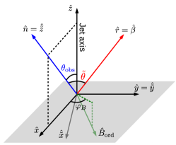
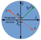
Figure 1: Top: Illustration of the coordinate system in which the polarization vector associated to synchrotron emission is calculated. Here the direction of the local bulk velocity is $\hat{\beta}=\hat{r}$ and the direction of the uniform magnetic field is transverse to that with azimuthal angle $\varphi_{B}$. The polar angle $\tilde{\theta}$ in the lab-frame is between the directions of the local bulk velocity and observed photon, with $\tilde{\mu}\equiv\cos\tilde{\theta}=\hat{n}\cdot\hat{\beta}$. Bottom: The observer sees the projection of the ordered magnetic field (green arrow) and polarization vector (red arrow) on the plane of the sky (shaded blue region; orthogonal to the direction of the wave vector $\hat{n}$ of the observed photon, which points out of the page). For an ordered magnetic field the polarization position angle $\theta_{p}$ is measured from the direction of the ordered field (solid arrow), otherwise $\theta_{p}$ is measured from the projection of the jet symmetry axis (dashed arrow).

The measured Stokes parameters are a sum over the flux $dF_{\nu}$ contributed by individual fluid elements, which yields (e.g. Granot, 2003)

$$\left\{\begin{array}[]{c}U/I\\ Q/I\end{array}\right\}=\left(\int dF_{\nu}\right)^{-1}\int dF_{\nu}\left\{\begin{array}[]{c}\Pi^{\prime}\sin 2\theta_{p}\\ \Pi^{\prime}\cos 2\theta_{p}\end{array}\right\}~{},$$ (5)

where

$$dF_{\nu}(t_{\rm obs},\hat{n},r,t)=\frac{(1+z)}{d_{L}^{2}}\delta_{D}^{2}j^{\prime}_{\nu^{\prime}}\delta(t-t_{\rm obs}-\hat{n}\cdot\vec{r}/c)dtdV$$ (6)

is the flux received from a source at a redshift $z$ with luminosity distance $d_{L}(z)$ emitting towards the observer in the direction of the unit vector $\hat{n}$. Here $j^{\prime}_{\nu^{\prime}}$ is the fluid-frame spectral emissivity, $dV$ is the lab-frame volume of the fluid element, and

$$\delta_{D}(r)=[\Gamma(1-\vec{\beta}\cdot{\hat{n}})]^{-1}=[\Gamma(1-\beta\tilde{\mu})]^{-1}$$ (7)

is the Doppler factor, where $\hat{n}\cdot\hat{\beta}=\cos\tilde{\theta}\equiv\tilde{\mu}$ and $\tilde{\theta}$ is the polar angle measured from the LOS. The delta-function term $\delta(t-t_{\rm obs}-\hat{n}\cdot\vec{r}/c)$ imposes the condition that for a given $t_{\rm obs}$ emission is received from an equal arrival time surface or volume depending on whether the emission is from a thin shell or a finite volume (e.g. Granot, Piran, & Sari, 1999a; Granot, Cohen-Tanugi, & Do Couto E Silva, 2008).

For simplicity, we ignore the radial structure of the outflow, and assume that the emission originates from an infinitely “thin-shell.” This approximation is valid if the timescale over which particles cool and contribute to the observed radiation is much smaller than the dynamical time. This implies that the emission region is a thin cooling layer of width (in the lab-frame) $\Delta\ll R/2\Gamma^{2}$. In this approximation, the flux density from each fluid element can be expressed as (Granot, 2005)

$$dF_{\nu}(t_{\rm obs},\hat{n},r)=\frac{(1+z)}{16\pi^{2}d_{L}^{2}}\delta_{D}^{3}L^{\prime}_{\nu^{\prime}}(r)d\tilde{\Omega}~{},$$ (8)

where $L^{\prime}_{\nu^{\prime}}(r)$ is the fluid-frame spectral luminosity and $d\tilde{\Omega}=d\tilde{\mu}~{}d\tilde{\varphi}$ is the solid angle subtended by the fluid element w.r.t. the central source (i.e. the origin of the two coordinate systems).

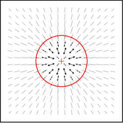
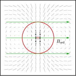
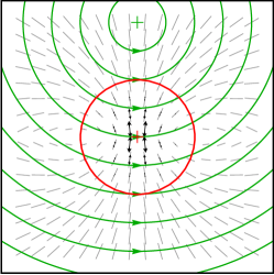
Figure 2: Local polarization map (shown for $\epsilon=1+\alpha=2$) for different magnetic field configurations (shown in green for the two locally ordered field cases): (Left) Random field $B_{\perp}$ in the plane of the ejecta (normal to the radial direction), (Middle) ordered field $B_{\rm ord}$, shown by green horizontal arrows, and (Right) toroidal field ($q\sqrt{\xi}_{j}=2$ with $\sqrt{\xi}_{j}\gtrsim 4.5$; $q\equiv\theta_{\rm obs}/\theta_{j}$ and $\xi_{j}\equiv(\Gamma\theta_{j})^{2}$), where the jet symmetry axis is marked with a green ‘+’ sign. The red circle shows the boundary ($\tilde{\xi}^{1/2}=\Gamma\tilde{\theta}=1$) of the region in the jet whose beaming cone includes our line of sight ($\tilde{\xi}=0$, marked with red ‘+’ sign), projected on the plane of the sky. The magnitude of the black arrows reflects the polarized intensity and the gray line segments show the same but normalized by $\delta_{D}^{(3+\alpha)}$. See also Granot & Ramirez-Ruiz (2011).

The anisotropic synchrotron spectral luminosity is expressed as (e.g. Rybicki & Lightman, 1979)

$$L^{\prime}_{\nu^{\prime}}(r)\propto(\nu^{\prime})^{-\alpha}(\sin\chi^{\prime})^{\epsilon}r^{m}\propto(\nu^{\prime})^{-\alpha}[1-(\hat{n}^{\prime}\cdot\hat{B}^{\prime})^{2}]^{\epsilon/2}r^{m}$$ (9)

where we assume a power law spectrum and power law dependence of the emissivity on $r$. Here $\chi^{\prime}$ is the angle between the direction of the local magnetic field and emitted photon. Since synchrotron emission from relativistic electrons is highly beamed in the direction of motion, $\chi^{\prime}$ is also the pitch angle between the electron’s velocity vector and the magnetic field. The power law index $\epsilon$ depends on the electron energy distribution, and if the latter is independent of the pitch angles then $\epsilon=1+\alpha$. In the rest of this work, we only consider a constant emissivity with radius ($m=0$).

The degree to which the synchrotron emission is polarized depends on the underlying distribution of the emitting electrons, both in energy and pitch angle $\chi^{\prime}$. We consider an isotropic electron velocity and a power law distribution in energy, with the number density of electrons scaling as $n_{e}(\gamma_{e})\propto\gamma_{e}^{-p}$. In this case, the maximum degree of linear polarization from a fluid element with an ordered field is

$$\Pi_{\rm max}=\frac{\alpha+1}{\alpha+5/3}=\frac{p_{\rm eff}+1}{p_{\rm eff}+7/3}~{},$$ (10)

where $\alpha=(p_{\rm eff}-1)/2$, and for optically-thin synchrotron emission $\alpha\geq-1/3$ which yields $\Pi_{\rm max}\geq 1/2$. The value of $p_{\rm eff}$ changes depending on the different power law segments (e.g. Granot & Sari, 2002) of the synchrotron flux density, such that $p_{\rm eff}=\{2,p,p+1\}$ corresponding to $\alpha=\{1/2,(p-1)/2,p/2\}$ and PLSs {F, G, H}. For PLSs D and E, for which $\alpha=-1/3$, $\Pi_{\rm max}=1/2$ as the emission here arises from all electrons below their synchrotron frequency and therefore these PLSs have the lowest (optically-thin) level of polarization.

For a tangled or random field, the local degree of polarization from a given point on the emitting thin shell, after averaging over all directions of the random magnetic field, and under the simplifying assumption that $\epsilon=2$, is given by (Sari, 1999; Gruzinov, 1999; Granot & Königl, 2003)

$$\frac{\Pi_{\rm rnd}^{\prime}(\tilde{\theta}^{\prime})}{\Pi_{\rm max}} =\frac{(b-1)\sin^{2}\tilde{\theta}^{\prime}}{2+(b-1)\sin^{2}\tilde{\theta}^{\prime}}\quad\quad(\epsilon=2)$$ (14)

$$=\left\{\begin{array}[]{cc}\displaystyle\frac{-\sin^{2}\tilde{\theta}^{\prime}}{1+\cos^{2}\tilde{\theta}^{\prime}}&(b=0~{},B\to B_{\perp})\\ \\ 1&(b\to\infty~{},B\to B_{\parallel})\end{array}\right.$$

The above result can be expressed in terms of the lab-frame angles through the aberration of light, such that

$$\cos\tilde{\theta}^{\prime}\equiv\tilde{\mu}^{\prime}=\frac{\tilde{\mu}-\beta}{1-\beta\tilde{\mu}}~{}.$$ (15)

To obtain the direction of the polarization vector on the plane of the sky, we start by defining the unit-vector $\hat{n}$ in the direction of the emitted photon in the lab frame. It is expressed using a coordinate system with $\hat{z}$ along the jet symmetry axis (as shown in Fig. 1), such that $\hat{n}=\sin\theta_{\rm obs}~{}\hat{x}+\cos\theta_{\rm obs}~{}\hat{z}$, where $\varphi_{B}$ is the azimuthal angle of the ordered magnetic field that is transverse to the radial vector. For synchrotron radiation, the polarization unit-vector in the fluid-frame $\hat{e}^{\prime}=\hat{B}^{\prime}\times\hat{n}^{\prime}/|B^{\prime}\times\hat{n}^{\prime}|$ is orthogonal to both the direction of the local magnetic field and that of the emitted photon, both expressed in the frame of the radiating element moving with velocity $\vec{\beta}c$. In the lab-frame, the orientation of the polarization vector is obtained by the following Lorentz transformation (see, e.g. Lyutikov, Pariev, & Blandford, 2003)

$$\hat{e}=\frac{\displaystyle\hat{e}^{\prime}+\Gamma\vec{\beta}\left[\frac{\Gamma}{\Gamma+1}(\hat{e}^{\prime}\cdot\vec{\beta})+1\right]}{\displaystyle\Gamma(1+\hat{e}^{\prime}\cdot\vec{\beta})}~{}.$$ (16)

The direction of polarization naturally lies on the plane of the sky (i.e. $\hat{e}\cdot\hat{n}=0$), with $\hat{e}=(\hat{e}\cdot\hat{\tilde{x}})\hat{\tilde{x}}+(\hat{e}\cdot\hat{\tilde{y}})\hat{\tilde{y}}$, where $\hat{\tilde{x}}=\cos\theta_{\rm obs}\hat{x}-\sin\theta_{\rm obs}\hat{z}$, $\hat{\tilde{y}}=\hat{y}$, and $\hat{\tilde{z}}=\hat{n}$.

When the magnetic field is completely tangled, for $b>1$ ($b<1$) the local polarization is $\Pi_{\rm rnd}^{\prime}>0$ ($\Pi_{\rm rnd}^{\prime}<0$) and the direction of the polarization vector is along (normal to) the direction of $\hat{n}^{\prime}\times\hat{r}$.

3.3 Effects of LOS and magnetic field configuration

First we present general expressions that are valid for both on and off-axis observers. Then, in the subsequent sections we discuss the expected degree of polarization measured by an on-axis observer (§3.4) for different magnetic field configurations, and by off-axis observers (§3.5).

In the ultra-relativistic limit ($\Gamma\gg 1$), approximate expressions accurate to $\mathcal{O}(\Gamma^{-2})$ may be used. In this limit, the Doppler factor is given by

$$\delta_{D}\approx\frac{2\Gamma}{(1+\tilde{\xi})}\quad\quad{\rm where}\quad\quad\tilde{\xi}\equiv(\Gamma\tilde{\theta})^{2}~{},$$ (17)

using the approximations $\tilde{\mu}\equiv\cos\tilde{\theta}\approx 1-\tilde{\theta}^{2}/2$, and $\beta\approx 1-1/(2\Gamma^{2})$. From the definition of the unit-vector $\hat{n}$, and using the aberration of light, the factor related to the pitch angle in Eq. (9),

$$\Lambda\equiv\langle[1-(\hat{n}^{\prime}\cdot\hat{B}^{\prime})^{2}]^{\epsilon/2}\rangle~{},$$ (18)

where the averaging is over the local probability distribution of $\hat{B}^{\prime}$, can be expressed as follows for different field orientations,

$$({\rm i})\quad \Lambda_{\rm ord} \approx\left[\left(\frac{1-\tilde{\xi}}{1+\tilde{\xi}}\right)^{2}\cos^{2}\varphi_{B}+\sin^{2}\varphi_{B}\right]^{\epsilon\over 2}$$

$$({\rm ii})\quad \Lambda_{\perp} =\langle\Lambda_{\rm ord}(\tilde{\xi},\varphi_{B})\rangle_{\varphi_{B}}$$

$$({\rm iii})\quad \Lambda_{\parallel} \approx\left[\frac{\sqrt{4\tilde{\xi}}}{1+\tilde{\xi}}\right]^{\epsilon}$$ (19)

$$({\rm iv})\quad \Lambda_{\rm tor} \approx\left[\left(\frac{1-\tilde{\xi}}{1+\tilde{\xi}}\right)^{2}+\frac{4\tilde{\xi}}{(1+\tilde{\xi})^{2}}\frac{(a+\cos\tilde{\varphi})^{2}}{(1+a^{2}+2a\cos\tilde{\varphi})}\right]^{\epsilon\over 2}\,,$$

for (i) $B_{\rm ord}$ that is in the plane of the ejecta, (ii) for the $B_{\perp}$ case we average $\Lambda_{\rm ord}$ over the uniform distribution of $\varphi_{B}$ within the plane of the ejecta (see Eq. (36) and the discussion in §3.5.2); (iii) $B_{\parallel}$, and (iv) $B_{\rm tor}$, for which $a\equiv\tilde{\theta}/\theta_{\rm obs}$. In the above, the angle $\varphi_{B}$ is measured from some reference direction and $\tilde{\varphi}$ is measured from the projection of the jet symmetry axis on the plane of the sky (see Fig. 1 for reference).

The polarization angle in the limit $\Gamma\gg 1$ is given by Granot & Königl (2003); Granot (2003); Granot & Taylor (2005)

$$({\rm i})\quad\theta_{p} = \varphi_{B}+\arctan\left[\left(\frac{1-\tilde{\xi}}{1+\tilde{\xi}}\right)\cot\varphi_{B}\right]$$ (20)

$$({\rm ii})\quad\theta_{p} = \tilde{\varphi}$$ (21)

$$({\rm iii})\quad\theta_{p} = \left\{\begin{array}[]{cc}0~{},&\Pi^{\prime}>0\\ \pi/2~{},&\Pi^{\prime}<0\end{array}\right.$$ (24)

$$({\rm iv})\quad\theta_{p} = \tilde{\varphi}-\arctan\left[\left(\frac{1-\tilde{\xi}}{1+\tilde{\xi}}\right)\frac{\sin\tilde{\varphi}}{a+\cos\tilde{\varphi}}\right]\ ,$$ (25)

where for the ordered field (case (i)) $\theta_{p}$ is measured from the local direction of the magnetic field, otherwise it is measured from the projection of the jet symmetry axis on the plane of the sky. For the direction of the PA when the magnetic field is tangled in the plane of the ejecta ($B_{\perp}$), see the discussion in §3.5.2.

3.4 On-Axis Observer

3.4.1 Top-hat jet viewed on-axis

When the jet is ultra-relativistic ($\Gamma\gg 1$) the observer mainly receives photons from within a cone of semi-aperture (or beaming angle) $\tilde{\theta}=\Gamma^{-1}$ around the LOS due to relativistic beaming. Generally, $\Gamma\theta_{j}\gtrsim 10$ and therefore the edge of the jet is not yet visible to an on-axis observer ($\theta_{\rm obs}=0$). In this case, the emission from the jet can be approximated as arising from an expanding thin spherical shell. The edge only becomes visible when the ejecta has slowed down significantly to $\Gamma\sim\theta_{j}^{-1}$, which happens around the time of the jet break.

In the left and middle panels of Fig. 2 we show the polarization map for an on-axis observer. Here the length of the double-arrowed vectors shown in black represent the polarized intensity and the line segments in gray show the same but normalized by the Doppler factor term $\delta_{D}^{(3+\alpha)}$ that rapidly suppresses the intensity. This behaviour is more clearly shown in Fig. 3 along with the local degree of polarization and polarized intensity as a function of $\tilde{\xi}$ for $B_{\perp}$ magnetic field configuration.

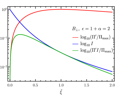
Figure 3: Comparison (for a spherical relativistic uniform emitting shell) of the local degree of polarization, $\Pi^{\prime}=\Pi_{\rm rnd}^{\prime}$ from Eq. (14) for $b=0$, with the polarized intensity $\Pi^{\prime}I$, where $I$ is the intensity (obtained by averaging over the random magnetic field directions; see Eq. (36)) normalized by its value along the line of sight [$\tilde{\xi}=(\Gamma\tilde{\theta})^{2}=0$].

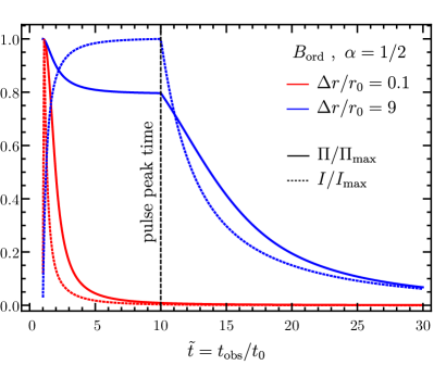
Figure 4: Temporal evolution of the degree of polarization and intensity over a single pulse, shown here for an ordered magnetic field in the plane of the ejecta, for a spherical relativistic uniform emitting shell (after Nakar, Piran, & Waxman, 2003). However, when integrated over the entire pulse, both cases yield the same polarization.

3.4.2 Temporal evolution over a single pulse

The degree of polarization varies over the duration of a single pulse as emission from different radii and polar angles away from the LOS contribute to the flux at a given observer time $t_{\rm obs}$. In order to account for this effect, an integration over the equal arrival time surface (EATS) must be carried out (e.g. Granot, Piran, & Sari, 1999a; Granot, Cohen-Tanugi, & Do Couto E Silva, 2008). In general, the emissivity and the spectrum can also vary over the single pulse, which would affect the level of polarization. Here, however, we explicitly assume, for simplicity, a constant emissivity and no spectral changes. More complex evolution of both and their effect on the time-resolved degree of polarization will be explored in a future work.

In the thin-shell approximation, after a lab-frame time $t$ the shell has moved a radial distance $r=\beta ct\approx ct$. In this case the EATS condition dictates that

$$t_{{\rm obs},z}\equiv\frac{t_{\rm obs}}{1+z}=t-\frac{r\tilde{\mu}}{c}=\frac{(1-\beta\tilde{\mu})}{\beta}\frac{r}{c}\approx\frac{(1+\tilde{\xi})}{2\Gamma^{2}}\frac{r}{c}~{},$$ (26)

where the last expression is only valid in the ultra-relativistic limit. We further assume that the thin-shell starts radiating at radius $r=r_{0}$ and has a constant luminosity until the radius $r=r_{0}+\Delta r$, beyond which the emission stops. From the EATS equation, it is simple to deduce that for a given $t_{{\rm obs},z}$, only radii $r_{\rm min}\leq r\leq r_{\rm max}$, corresponding to $-1\leq\mu\leq 1$, can contribute to the observed flux, where

$$r_{\rm min} = \max\left(r_{0}~{},~{}\frac{\beta ct_{{\rm obs},z}}{1+\beta}\right)\approx\max\left(r_{0}~{},~{}\frac{ct_{{\rm obs},z}}{2}\right)$$ (27)

$$r_{\rm max} = \min\left(r_{0}+\Delta r~{},~{}\frac{\beta ct_{{\rm obs},z}}{1-\beta}\right)\approx\min\left(r_{0}+\Delta r~{},~{}2\Gamma^{2}ct_{{\rm obs},z}\right)\quad\quad$$ (28)

Plugging these conditions into Eq. (26), we find that $\tilde{\xi}_{\min}\leq\tilde{\xi}\leq\tilde{\xi}_{\max}$, where

$$\tilde{\xi}_{\min}=\max\left[0~{},~{}\left(1+\frac{\Delta r}{r_{0}}\right)^{-1}\tilde{t}-1\right]\quad{\rm and}\quad\tilde{\xi}_{\max}=\tilde{t}-1~{},$$ (29)

with $\tilde{t}\equiv t_{\rm obs}/t_{0}$. Here $t_{0}\equiv(1+z)r_{0}/(2\Gamma^{2}c)$ is the time of reception of the first photon, which is also equivalent to the angular time $t_{\rm obs,\theta}$ at $r_{0}$ within which photons from an area with angular size $\tilde{\theta}=1/\Gamma$ are received after the reception of the first photon. Then, integration over the EATS yields (e.g. Nakar, Piran, & Waxman, 2003) the general equation for the Stokes parameters,

$$\left\{\begin{array}[]{c}\displaystyle\frac{U(\tilde{t})}{I(\tilde{t})}\\ \\ \displaystyle\frac{Q(\tilde{t})}{I(\tilde{t})}\end{array}\right\}=\frac{\displaystyle\int_{\tilde{\xi}_{\min}(\tilde{t})}^{\tilde{\xi}_{\max}(\tilde{t})}\frac{d\tilde{\xi}}{(1+\tilde{\xi})^{3+\alpha}}\int d\tilde{\varphi}\Lambda(\tilde{\xi},\tilde{\varphi})\left\{\begin{array}[]{c}\Pi^{\prime}\sin 2\theta_{p}\\ \Pi^{\prime}\cos 2\theta_{p}\end{array}\right\}}{\displaystyle\int_{\tilde{\xi}_{\min}(\tilde{t})}^{\tilde{\xi}_{\max}(\tilde{t})}\frac{d\tilde{\xi}}{(1+\tilde{\xi})^{3+\alpha}}\int d\tilde{\varphi}\Lambda(\tilde{\xi},\tilde{\varphi})}~{}.$$ (30)

In Fig. 4, we show the temporal evolution of the degree of polarization as well as intensity over a single pulse. We show two cases where $\Delta r/r_{0}=0.1$ and $\Delta r/r_{0}=9$ (corresponding to $r_{f}/r_{0}=t_{f}/t_{0}=(1+\Delta r/r_{0})=10$, and explaining why the peak time is at $\tilde{t}=t_{\rm obs}/t_{0}=10$). In the former, the initial angular time $t_{\rm obs,\theta}=t_{0}$ dominates over the radial time $t_{{\rm obs},r}=(1+z)\Delta r/(2\Gamma^{2}c)$ since $\Delta r\ll r_{0}$. In the latter the radial time dominates over the initial angular time, while the final angular time at a radius $r_{f}=r_{0}+\Delta r$ dominates the decaying part of the flux after it peaks. In both cases, the degree of polarization is maximum ($\Pi=\Pi_{\max}$) at the beginning of the pulse since only photons originating along the LOS are observed. However, as photons from larger angles away from the LOS are observed, the level of polarization declines. A sharper decline in $\Pi/\Pi_{\max}$ is seen after the peak of the pulse when high latitude emission dominates.

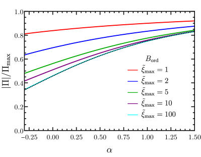
Figure 5: Degree of polarization when the magnetic field is ordered ($B_{\rm ord}$), shown for different values of $\tilde{\xi}_{\rm max}=(\Gamma\theta_{\max})^{2}$ from Eq. (31). In the limit $\tilde{\xi}_{\rm max}\to\infty$, $\Pi$ approaches that obtained from explicit time integration over a single pulse, which is shown by the black dotted line (after Granot, 2003). The jet geometry is that of a spherical flow since most of the contribution arises from a region of angular size $1/\Gamma$ around the LOS. Contribution from larger angles (or correspondingly larger $\tilde{\xi}$) is suppressed by relativistic beaming. For optically-thin synchtrotron emission $-1/3\leq\alpha<p/2$ for the electron energy distribution power law index $2\lesssim p\lesssim 3$; see Eq. (10) and the discussion that follows.

3.4.3 Pulse integrated polarization

In the case of prompt emission, the measured polarization is generally integrated over at least a single pulse, if not multiple pulses (see §6). The pulse integrated Stokes parameters, e.g. the total intensity which is proportional to the fluence over a single pulse can be obtained using $dF_{\nu}dt_{\rm obs}\propto\Delta t^{\prime}\delta_{D}^{2}L^{\prime}_{\nu^{\prime}}d\tilde{\Omega}$, where $\Delta t^{\prime}=\delta_{D}dt_{\rm obs}$ is the duration of the pulse in the comoving frame (see Appendix A for more details). This amounts to reducing one power of the Doppler factor in Eq. (30), and therefore the pulse integrated polarization can now be conveniently expressed as (Granot, 2003),

$$\left\{\begin{array}[]{c}U/I\\ Q/I\end{array}\right\}=\frac{\displaystyle\int\frac{d\tilde{\xi}}{(1+\tilde{\xi})^{2+\alpha}}\int d\tilde{\varphi}\Lambda(\tilde{\xi},\tilde{\varphi})\left\{\begin{array}[]{c}\Pi^{\prime}\sin 2\theta_{p}\\ \Pi^{\prime}\cos 2\theta_{p}\end{array}\right\}}{\displaystyle\int\frac{d\tilde{\xi}}{(1+\tilde{\xi})^{2+\alpha}}\int d\tilde{\varphi}\Lambda(\tilde{\xi},\tilde{\varphi})}~{}.$$ (31)

When doing an explicit time integration in Eq. (30) another simplification can be made. Since the total polarization should not depend on the duration over which the radiating shell is active or equivalently $\Delta r$, a delta function in $r$ can be assumed by taking $\Delta r\to 0$. This can also be noticed from Fig. 4, where integration over both curves yields the same polarization given a sufficiently large upper limit on $\tilde{t}$ when integrating where the polarized intensity vanishes. This effectively implies integrating over the outflow surface at a fixed radius for $0\leq\tilde{\xi}\leq\tilde{\xi}_{\max}$, with no dependence on $t_{\rm obs}$, and $0\leq\tilde{\varphi}\leq 2\pi$. Therefore, any temporal evolution of the luminosity within a pulse does not affect the time-integrated degree of polarization when all else remains the same.

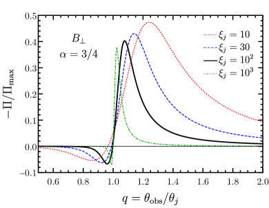
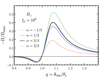
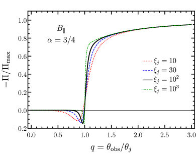
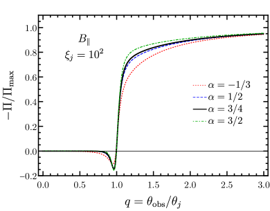
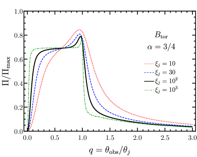
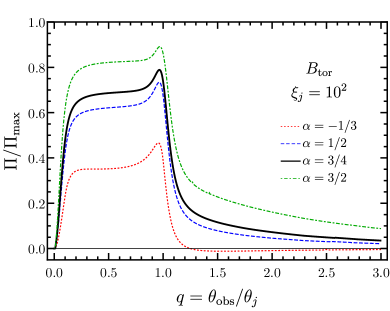
Figure 6: Pulse integrated degree of polarization arising from a top-hat jet for (top) a random magnetic field ($B_{\perp}$) that is normal to the local velocity vector, $\vec{\beta}$, and lies entirely in the plane of the ejecta, (middle) a locally ordered field ($B_{\parallel}$) with direction parallel to $\vec{\beta}$, and (bottom) a globally ordered toroidal field ($B_{\rm tor}$). All are shown for various values of $\xi_{j}=(\Gamma\theta_{j})^{2}$ (left panel) and different values of the spectral index $\alpha$ (right panel) (after Granot, 2003; Granot & Taylor, 2005).

From symmetry considerations $U=0$ and the degree of polarization is $\Pi=|Q|/I$. The value of $\tilde{\xi}_{\rm max}=(\Gamma\tilde{\theta}_{\rm max})^{2}$ determines the maximal angle from the LOS ($\tilde{\theta}_{\rm max}$ in units of $1/\Gamma$) out to which the contribution to the observed flux is included. For a spherical shell and if the flux is integrated well into the tail of the pulse, this would correspond to $\tilde{\xi}_{\rm max}\gg 1$. If, on the other hand, we measure the polarization of a pulse (of width $\Delta t_{\rm obs}$ and peak time $t_{p}$) over a time interval $t_{1}<t_{\rm obs}<t_{2}$ that contains only part of its tail (but all of its rising part), this would effectively correspond to a finite $\tilde{\xi}_{\rm max}\sim 1+(t_{2}-t_{p})/\Delta{t_{\rm obs}}$. This arises since the emission at $t_{\rm obs}\sim t_{p}$ is dominated by the contribution from $\tilde{\xi}\sim 1$, while during the tail it is predominantly from $\tilde{\xi}\sim 1+(t_{\rm obs}-t_{p})/\Delta{t_{\rm obs}}$. Finally, even if the integration time extends well into the tail of the pulse, $(t_{2}-t_{p})/\Delta{t_{\rm obs}}\gg 1$, then a line of sight close to the edge of the jet, or a rather narrow jet, can again introduce an effective $\tilde{\xi}_{\rm max}=(\Gamma\tilde{\theta}_{\rm max})^{2}$.

In Fig. 5, we show the time-integrated (over the duration of a single pulse) degree of polarization arising from a spherical shell with an ordered magnetic field in the plane normal to $\vec{\beta}$, where for large $\tilde{\xi}_{\max}\sim 100$ the result converges to that obtained by explicitly integrating over the entire pulse duration.

For an on-axis observer ($\theta_{\rm obs}=0$), if the magnetic field configuration is toroidal or random, the degree of polarization averaged over the GRB image vanishes due to the inherent axisymmetry of the outflow around the LOS. To break the symmetry, the jet must be viewed off-axis ($\theta_{\rm obs}>0$). In the case of the toroidal field, the geometry of the field is sufficient to break the symmetry, however, for a random field that is symmetric around the LOS the outflow must be sufficiently inhomogeneous in its properties as a function of $\theta$ from the jet axis, e.g. in (i) a top-hat jet where the jet is uniform within the initial jet half-opening angle $\theta_{j}$ beyond which the emissivity drops abruptly, effectively giving the outflow a sharp edge, or (ii) in a structured jet, where the emissivity $L^{\prime}_{\nu^{\prime}}=L^{\prime}_{\nu^{\prime}}(\theta)$ and/or the bulk LF $\Gamma=\Gamma(\theta)$ vary smoothly with $\theta$ outside of a compact core that has an angular size $\theta_{c}$.

3.5 Off-Axis Observer

3.5.1 Top-hat jet viewed off-axis – Ordered magnetic field

Here we discuss the degree of polarization obtained from ordered fields, such as a toroidal field ($B_{\rm tor}$) and a field ($B_{\parallel}$) that is parallel to the local velocity vector $\vec{\beta}$ which is assumed to be radial. In the toriodal field case, when the jet is viewed on-axis ($\theta_{\rm obs}=0$), the total polarization averaged over the GRB image vanishes. Therefore, the observer’s LOS must be off-axis, $\theta_{\rm obs}>0$. The local polarization from a given point of the observed image on the plane of the sky is exactly the same as that from an ordered field that is entirely in the plane of the ejecta, however, the global structure of the magnetic field adds more complexity (see right panel of Fig. 2). Therefore, after integrating over the solid angle subtended by the source, we find (Granot & Taylor, 2005) a time-integrated polarization

$$\frac{\Pi}{\Pi_{\rm max}}= \displaystyle\left[H(1-q)\int_{0}^{\xi_{-}}\frac{d\tilde{\xi}}{(1+\tilde{\xi})^{2+\alpha}}\int_{0}^{2\pi}d\tilde{\varphi}\Lambda_{\rm tor}(\tilde{\xi},\tilde{\varphi},a)\cos 2\theta_{p}\right.$$

$$\displaystyle+\left.\int_{\xi_{-}}^{\xi_{+}}\frac{d\tilde{\xi}}{(1+\tilde{\xi})^{2+\alpha}}\int_{\psi}^{2\pi-\psi}d\tilde{\varphi}\Lambda_{\rm tor}(\tilde{\xi},\tilde{\varphi},a)\cos 2\theta_{p}\right]$$

$$\times\displaystyle\left[H(1-q)\int_{0}^{\xi_{-}}\frac{d\tilde{\xi}}{(1+\tilde{\xi})^{2+\alpha}}\int_{0}^{2\pi}d\tilde{\varphi}\Lambda_{\rm tor}(\tilde{\xi},\tilde{\varphi},a)\right.$$

$$\displaystyle+\left.\int_{\xi_{-}}^{\xi_{+}}\frac{d\tilde{\xi}}{(1+\tilde{\xi})^{2+\alpha}}\int_{\psi}^{2\pi-\psi}d\tilde{\varphi}\Lambda_{\rm tor}(\tilde{\xi},\tilde{\varphi},a)\right]^{-1}$$

where $H(1-q)$ is the Heaviside step-function, and

$$\cos\psi(\tilde{\xi})=\frac{\displaystyle(1-q^{2})\xi_{j}-\tilde{\xi}}{\displaystyle 2q\sqrt{\tilde{\xi}\xi_{j}}}$$ (33)

$$q=\theta_{\rm obs}/\theta_{j}~{},\quad\xi_{j}=(\Gamma\theta_{j})^{2}~{},\quad\xi_{\pm}=(1\pm q)^{2}\xi_{j}~{}.$$ (34)

The bottom panel of Fig. 6 shows the pulse-integrated $\Pi$ for a toroidal field. The degree of polarization vanishes for $q=0$ due to symmetry, but remains high for $\xi_{j}^{-1/2}\lesssim q\lesssim 1+\xi_{j}^{-1/2}$, and drops sharply for $q>1$.

The calculation for the $B_{\parallel}$ case follows from that presented in Granot (2003), where the total polarization for an off-axis observer is obtained from

$$\Pi=\frac{\displaystyle\frac{1}{2\pi}\int_{\xi_{-}}^{\xi_{+}}\frac{d\tilde{\xi}}{(1+\tilde{\xi})^{2+\alpha}}\Lambda(\tilde{\xi})\Pi_{\max}\sin 2\psi(\tilde{\xi})}{\displaystyle H(1-q)\int_{0}^{\xi_{-}}\frac{d\tilde{\xi}\Lambda(\tilde{\xi})}{(1+\tilde{\xi})^{2+\alpha}}+\int_{\xi_{-}}^{\xi_{+}}d\tilde{\xi}\frac{\pi-\psi(\tilde{\xi})}{\pi(1+\tilde{\xi})^{2+\alpha}}\Lambda(\tilde{\xi})}~{},$$ (35)

where $\Lambda(\tilde{\xi})=\Lambda_{\parallel}(\tilde{\xi})$ from Eq. (3.3). The result of the integration are presented in the middle panel of Fig. 6, where the left panel shows the variation in $\Pi$ as the jet becomes narrow or wide, and the right panel shows dependence of $\Pi$ on the spectral index. Softer spectra tend to be more polarized and this trend applies to synchrotron emission regardless of the magnetic field configuration. The degree of polarization remains small for $q\lesssim 1-\xi_{j}^{-1/2}$, but sharply increases above $q=1$ and becomes large for $q\gtrsim 1+\xi_{j}^{-1/2}$. However, an important point to note here is that for $q>1+\xi_{j}^{-1/2}$, the fluence rapidly drops and such high levels of polarization in off-axis jets may only be realizable in nearby bursts. For bursts that are truly cosmological, one can only measure high $\Pi$ from this type of an ordered field for a very special geometry where $q\approx 1+\xi_{j}^{-1/2}$. The PA undergoes a change by $90^{\circ}$ around $q=1$, and the exact value of $q$ at which the polarization curve passes $\Pi=0$ depends on $\xi_{j}$, which suggests that if $\Gamma$ varies between different pulses and $q\sim 1$ then the observer may measure a $90^{\circ}$ shift in the PA. A similar behavior is observed for $B_{\perp}$ field case which is discussed next.

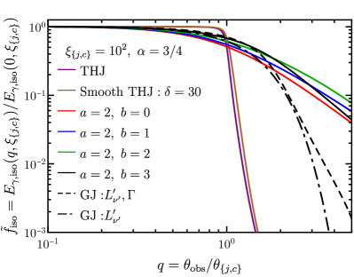
Figure 7: Ratio of off-axis to on-axis fluence, or equivalently isotropic equivalent energies, as a function of the ratio of the viewing angle $\theta_{\rm obs}$ to the half jet opening or core angle $\theta_{\{j,c\}}$. Shown here for different jet structures: a top-hat jet (THJ); smooth THJ ($\delta=30$; see Eq (48)); power law structured jet (PLJ; with $a=2$ and variable $b$; see Eq. (50)); and Gaussian structured Jet (GJ; with either both $L^{\prime}_{\nu^{\prime}}$ and $\Gamma$ varying as a Gaussian or only $L^{\prime}_{\nu^{\prime}}$; see Eq. (49)).

3.5.2 Top-hat jet viewed off-axis – Random magnetic field

When the magnetic field orientation is random in the plane of the ejecta, the observed polarization from an unresolved source vanishes upon averaging over the image on the plane of the sky (see left panel of Fig. 2). This occurs due to the fact that there is no special orientation of the polarization vector and it is symmetric around the LOS. To break the symmetry in this case, the jet must be viewed close to its edge ($q\gtrsim 1-\xi_{j}^{-1/2}$), where missing emission from $\theta>\theta_{j}$ results in only partial cancellation of the polarization when averaged over the GRB image (e.g. Waxman, 2003).

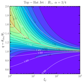
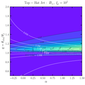
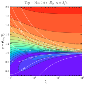
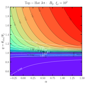
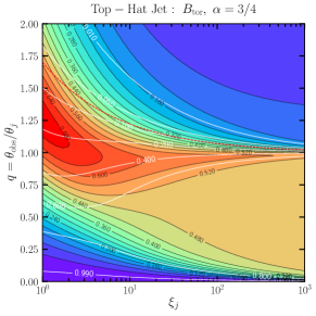
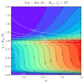
Figure 8: Contour plots of $|\Pi|$ for different magnetic field configurations: (top) random field entirely in the plane of the ejecta ($B_{\perp}$); (middle) ordered field parallel to the local velocity vector ($B_{\parallel}$); (bottom) toroidal field ($B_{\rm tor}$). The structure of the outflow is that of an ultra-relativistic top-hat jet. In the left panels $\alpha=3/4$ and the red dashed line shows $q=1+0.7/\sqrt{\xi_{j}}$, and in the right panels $\xi_{j}=(\Gamma\theta_{j})^{2}=10^{2}$. Contours for different values of $\tilde{f}_{\rm iso}$ are plotted in white.

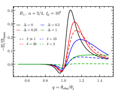
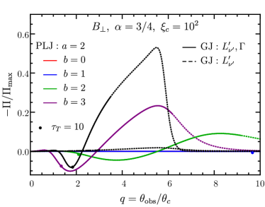
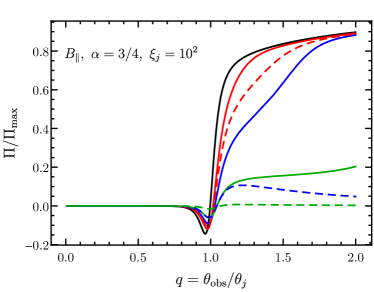
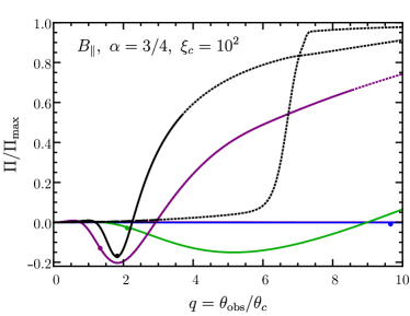
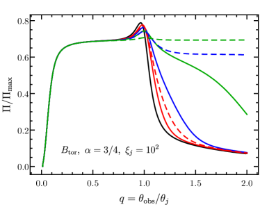
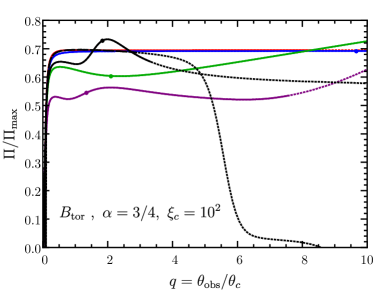
Figure 9: Left: Pulse integrated polarization of a smooth top-hat jet with a uniform core and exponential wings (solid lines) or power-law wings (dashed lines). Both are shown for different magnetic field configurations and for different smoothing parameters $\Delta$ and $\delta$, which control the rate at which the emissivity declines (after Nakar, Piran, & Waxman, 2003). Right: Pulse integrated degree of polarization for a structured jet – a power-law jet (PLJ) and gaussian jet (GJ) – shown for different field configurations. The dotted line shows the trend for large $q$ values but the pulses will be dim with $\tilde{f}_{\rm iso}<10^{-2}$. Furthermore, compactness arguments will restrict $q\lesssim 2$ for sufficiently steep profiles in all emission models (see §3.7.3 and Fig. 11), as shown by the filled circle obtained from Eq. (54) for the same fiducial parameters.

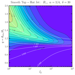
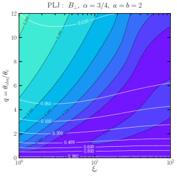
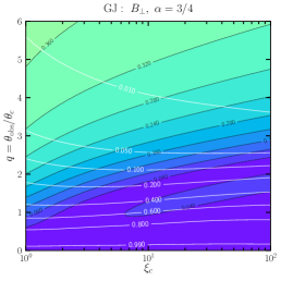
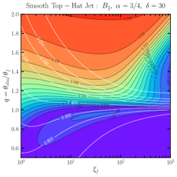
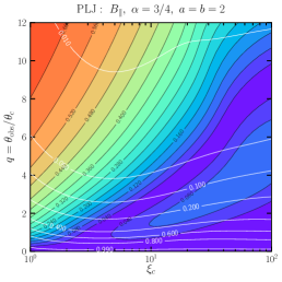
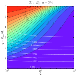
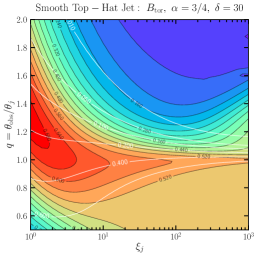
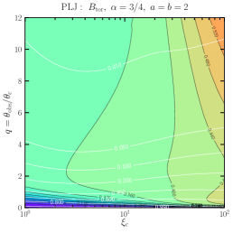
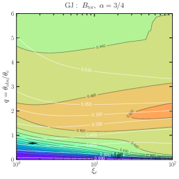
Figure 10: Contour plots of $|\Pi|$ for different magnetic field configurations and different jet structures. The left column shows the degree of polarization for a smooth top-hat jet, where the emissivity decays like a steep power law with smoothing parameter $\delta=30$. The center and right columns correspond to structured jets with emissivity $L^{\prime}_{\nu^{\prime}}(\theta)$ and $\Gamma(\theta)$ both having a power law ($a=b=2$; PLJ) and gaussian (GJ) profiles, respectively. The rows correspond to the different magnetic field configurations, with (top) a random field in the plane of the ejecta $B_{\perp}$, (middle) an ordered field in the direction parallel to the radial vector ($B_{\parallel}$), and (bottom) a globally ordered toroidal field ($B_{\rm tor}$). Contours for different values of $\tilde{f}_{\rm iso}$ are plotted in white.

The degree of polarization for an off-axis observer in this case is obtained from Eq. (35), where $\Lambda(\tilde{\xi})=\Lambda_{\perp}(\tilde{\xi})$ from Eq. (3.3). For $\epsilon=2$, we find from Eq. (14) that the local polarization from a given magnetic field element of $B_{\perp}$ is (in the limit $b\to 0$) $\Pi^{\prime}(\tilde{\xi})/\Pi_{\rm max}=-2\tilde{\xi}/(1+\tilde{\xi}^{2})$. In the general case, when $\epsilon\neq 2$, and for a random field that is in the plane transverse to the local velocity vector ($B_{\perp}$), the total polarization arising from a given fluid element has to be averaged over the various orientations of the magnetic field, which yields (using Eq. (1) of Sari, 1999)

$$\frac{\Pi_{\perp}^{\prime}(\tilde{\xi})}{\Pi_{\rm max}}=\frac{\displaystyle\frac{1}{\pi}\int_{0}^{\pi}\cos(2\theta_{p})\Lambda_{\perp}(\tilde{\xi},\varphi_{B})d\varphi_{B}}{\displaystyle\frac{1}{\pi}\int_{0}^{\pi}\Lambda_{\perp}(\tilde{\xi},\varphi_{B})d\varphi_{B}}~{},$$ (36)

where

$$\theta_{p}=\displaystyle\arctan\left[\left(\frac{1-\tilde{\xi}}{1+\tilde{\xi}}\right)\cot\varphi_{B}\right]~{},$$ (37)

$$\cos(2\theta_{p})=\displaystyle\left[\sin^{2}\varphi_{B}-\left(\frac{1-\tilde{\xi}}{1+\tilde{\xi}}\right)^{2}\cos^{2}\varphi_{B}\right]\left[\displaystyle 1-\frac{4\tilde{\xi}\cos^{2}\varphi_{B}}{(1+\tilde{\xi})^{2}}\right]^{-1}~{},\quad$$ (38)

and $\varphi_{B}$ is measured from some reference direction to carry out the averaging. Plugging in the expression for $\cos(2\theta_{p})$ into eq. (36) finally yields (Granot, 2003)

$$\displaystyle\frac{\Pi_{\perp}^{\prime}(\tilde{\xi})}{\Pi_{\rm max}}=\left\{\int_{0}^{\pi}d\varphi_{B}\left[1-\frac{4\tilde{\xi}\cos^{2}\varphi_{B}}{(1+\tilde{\xi})^{2}}\right]^{\epsilon/2}\right\}^{-1}$$ (39)

$$\times\displaystyle\int_{0}^{\pi}d\varphi_{B}\left[1-\frac{4\tilde{\xi}\cos^{2}\varphi_{B}}{(1+\tilde{\xi})^{2}}\right]^{(\epsilon-2)\over 2}\left[\sin^{2}\varphi_{B}-\left(\frac{1-\tilde{\xi}}{1+\tilde{\xi}}\right)^{2}\cos^{2}\varphi_{B}\right]~{}.$$

In the top panel of Fig. 6, we show the pulse-integrated degree of polarization for the random magnetic field scenario where the field lies entirely in the plane of the ejecta ($B_{\perp}$) for a top-hat jet. Similar to the $B_{\parallel}$ case, the PA changes direction by $90^{\circ}$ around $q=1$. Also, $\Pi$ now shows two distinct peaks at $q\sim 1\pm\xi_{j}^{-1/2}$. If $\Pi<0$ ($\Pi>0$), then the polarization vector will lie along (normal to) the line connecting the LOS to the jet axis.

3.6 Degree of polarization Vs fluence

As mentioned earlier, in the case of a top-hat jet the fluence drops very rapidly for viewing angles outside of the sharp edges for which $q\equiv\theta_{\rm obs}/\theta_{j}>1$. This introduces a bias against distant off-axis GRBs due to the flux limitations of the detector; all high redshift GRBs that are observed during the prompt phase are observed within the jet aperture ($\theta_{\rm obs}\lesssim\theta_{j}+1/\Gamma\leftrightarrow q\lesssim 1+\xi_{j}^{-1/2}$). Such a limitation also introduces a bias against measuring high degrees of polarization in the prompt phase from distant off-axis GRBs for a given magnetic field configuration. For example, both $B_{\parallel}$ and $B_{\perp}$ field configurations suffer from this bias since $\Pi$ rises significantly when $q>1$ as compared to its value when $q<1$.

Consider a pulse or emission episode that originated from an emission region with LF $\Gamma$ or equivalently with $\xi_{j}$ for a fixed $\theta_{j}$, and observed at a viewing angle $\theta_{\rm obs}$ or equivalently at some $q$. The fluence $S$ of the pulse can be straightforwardly obtained from the flux density defined in Eq. (6), where $S_{\gamma}=\int dt_{\rm obs}\int_{\nu_{1}}^{\nu_{2}}d\nu F_{\nu}(t_{\rm obs})$. This can be further used to write the isotropic equivalent energy $E_{\gamma,\rm iso}=4\pi d_{L}^{2}(1+z)^{-1}S_{\gamma}$. Here for simplicity we assume a power law spectrum within the whole observed spectral range. A useful parameter to gauge the suppression in fluence for an off-axis observer is the ratio of the off-axis to on-axis fluence or equivalently the ratio of the off-axis to on-axis isotropic equivalent energies,

$$\tilde{f}_{\rm iso}\equiv\frac{E_{\gamma,\rm iso}(q,\xi_{j})}{E_{\gamma,\rm iso}(0,\xi_{j})}=\frac{\int_{0}^{\tilde{\xi}_{\max}}\int_{0}^{2\pi}d\tilde{\varphi}\delta_{D}^{2+\alpha}\Gamma(\theta)^{-1}\Lambda(\tilde{\xi},\tilde{\varphi})\mathcal{L}(\theta)}{\left[\int_{0}^{\tilde{\xi}_{\max}}\int_{0}^{2\pi}d\tilde{\varphi}\delta_{D}^{2+\alpha}\Gamma(\theta)^{-1}\Lambda(\tilde{\xi},\tilde{\varphi})\mathcal{L}(\theta)\right]_{q=0}}$$ (40)

where the expression on the r.h.s is general and applies to any jet structure (Granot et al., 2002; Yamazaki et al., 2003; Eichler & Levinson, 2004; Granot & Ramirez-Ruiz, 2011; Salafia et al., 2015; Beniamini & Nakar, 2018), including a top-hat jet, and synchrotron emission with any magnetic field configuration as well as Compton drag. The structure of the jet is encoded in the dependence of the LF $\Gamma(\theta)$ and the emissivity, through $\mathcal{L}(\theta)=L^{\prime}_{\nu^{\prime}}/L^{\prime}_{\nu^{\prime},0}$, on $\theta=\theta(q,\theta_{\{j,c\}}\tilde{\theta},\tilde{\varphi})$ (see below and Appendix A). In Fig. 7 we show the dependence of $\tilde{f}_{\rm iso}$ on $q$ for a given $\xi_{\{j,c\}}$ and for different jet structures, such as a top-hat jet, smoothed top-hat jet, and structured jets – power law and gaussian jets – that are discussed below in §3.7. For a top-hat jet $\tilde{f}_{\rm iso}$ drops very sharply for $q\gtrsim 1$, while in the case of a structured jet it decays more gradually, since the fluence is dominated by contribution from along the LOS rather than that from within the jet’s core which is strongly suppressed at large viewing angles. Fig. 8 shows contour plots of the degree of polarization arising in synchrotron emission for the different magnetic field configurations. In the left panel, we show contours of $|\Pi|$ and $\tilde{f}_{\rm iso}$ (shown with white contours) over the $q$ and $\xi_{j}$ parameter space with fixed $\alpha$. In the right panel, the same is shown over the $q$ and $\alpha$ parameter space while keeping $\xi_{j}$ fixed.

3.7 Polarization from structured jets

3.7.1 Top-hat jet with smooth edges

The notion that relativistic jets have sharp edges, e.g. the top-hat jet model, is highly idealized. It is conceivable that the emissivity does not fall sharply beyond some uniformly emitting core with angular size $\theta_{j}$, but instead it declines more gradually. Here we follow the discussion of Nakar, Piran, & Waxman (2003) and present two models of a smooth top-hat jet, that has a uniformly bright core with smoothly decaying wings:

1. Exponential wings - the emission falls off exponentially outside of the uniform core, such that

   $$\frac{L^{\prime}_{\nu^{\prime}}}{L^{\prime}_{\nu^{\prime},0}}=\left\{\begin{array}[]{cc}1&\xi\leq\xi_{j}~{},\\ &\\ \exp[(\sqrt{\xi_{j}}-\sqrt{\xi})/\Delta]&\xi>\xi_{j}~{},\end{array}\right.$$ (44)

   where $L^{\prime}_{\nu^{\prime},0}$ is the uniform spectral luminosity.

2. Power-law wings - the emission declines as a power law outside of the uniform core, such that

   $$\frac{L^{\prime}_{\nu^{\prime}}}{L^{\prime}_{\nu^{\prime},0}}=\left\{\begin{array}[]{cc}1&\xi\leq\xi_{j}~{},\\ &\\ \displaystyle\left(\frac{\xi}{\xi_{j}}\right)^{-\delta/2}&\xi>\xi_{j}~{}.\end{array}\right.$$ (48)

In both cases, only the spectral luminosity is allowed to vary with $\theta$, but the dynamics remain angle independent, such that $\Gamma(\theta)=\Gamma_{0}$.

In the left panel of Fig. 9, we show the degree of polarization for different magnetic field configurations and for the two models with exponential and power-law wings. In both cases, it is clear that a sharp drop in the emissivity outside of the uniformly bright core is needed to obtain a high level of polarization for the $B_{\perp}$ and $B_{\parallel}$ magnetic field scenarios (Nakar, Piran, & Waxman, 2003). However, an opposite trend is seen for the $B_{\rm tor}$ magnetic field case, where jets with a shallow gradients show high levels of polarization when $q>1$.

3.7.2 Structured jets

In a truly structured jet the bulk LF of the emitting region must also vary with $\theta$ away from the jet symmetry axis. Here we consider two popular models (Zhang & Mészáros, 2002; Kumar & Granot, 2003; Granot & Kumar, 2003; Rossi, Lazzati, & Rees, 2002; Rossi et al., 2004):

1. Gaussian Jet (GJ): Both the spectral luminosity and the kinetic energy of the emitting material per unit rest mass, $\Gamma-1$, have a gaussian profile with a characteristic core angle $\theta_{c}$:

   $$\frac{L^{\prime}_{\nu^{\prime}}}{L^{\prime}_{\nu^{\prime},0}}=\frac{\Gamma(\theta)-1}{\Gamma_{c}-1}=\max\left[\exp\left(-\frac{\theta^{2}}{2\theta_{c}^{2}}\right)~{},~{}\exp\left(-\frac{\theta_{*}^{2}}{2\theta_{c}^{2}}\right)\right]~{},$$ (49)

   where $\Gamma_{c}$ is the LF of the core and $\theta_{*}$ implies a floor, which corresponds to some finite $\beta_{\rm min}$, that is both physically motivated and numerically convenient, and is chosen to be sufficiently small so that it does not affect any of the results.

2. Power-law Jet (PLJ): The spectral luminosity and the kinetic energy per unit rest mass of the emitting material decay as a power law outside of the core:

   $$\frac{L^{\prime}_{\nu^{\prime}}}{L^{\prime}_{\nu^{\prime},0}}=\Theta^{-a}~{},\quad\frac{\Gamma(\theta)-1}{\Gamma_{c}-1}=\Theta^{-b}~{},\quad\quad\Theta\equiv\sqrt{1+\displaystyle\left(\frac{\theta}{\theta_{c}}\right)^{2}}$$ (50)

We calculate the degree of polarization for a structured jet by numerically integrating the general expressions that are presented in Appendix A. In doing so we make the explicit assumption that the comoving spectral luminosity as well as the spectrum remain constant with shell radius $r$ as it expands. In addition, we assume that the spectrum does not depend on the polar angle $\theta$. The results of the integration are shown in the right-panels of Fig. 9. To obtain high levels of polarization when the magnetic field configuration is that of $B_{\perp}$ or $B_{\parallel}$, sharp gradients in $\Gamma$ outside of an approximately uniform core are needed. However, the toroidal field case again shows an opposite trend where sharp gradients yield slightly lower levels of polarization. For a top-hat jet the fluence drops very rapidly outside of the uniform core, however, in a structured jet the observer has access to angular regions that are well outside the core with $q\gtrsim 2$. This is demonstrated in the right-panels of Fig. 9 with the use of a dotted line for which $\tilde{f}_{\rm iso}<10^{-2}$. In Fig. 10 we show contours of $|\Pi|$ and $\tilde{f}_{\rm iso}$ (shown in white) as a function of $q$ and $\xi_{j}$ or $\xi_{c}$ for synchrotron emission and for different magnetic field configurations and jet structures.

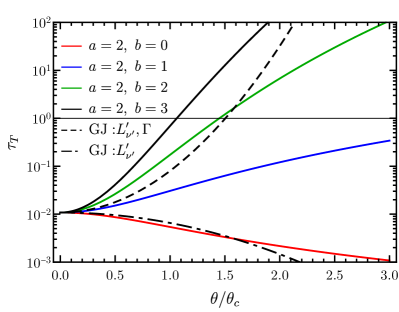
Figure 11: Thomson optical of $e^{-}e^{+}$-pairs produced (ignoring pair-annihilation) due to $\gamma\gamma$-annihilation of $\gamma$-ray photons when $\Gamma$ declines with polar angle from the jet symmetry axis. For a sufficiently steep angular profile for $\Gamma$, the prompt emission will be highly suppressed at $q=\theta_{\rm obs}/\theta_{c}\gtrsim 2$. See caption of Fig. 7 for legend labels.

3.7.3 Compactness limitation on $q$ in structured jets

In the case where the LF is not uniform and decreases away from the jet symmetry axis, the angular scale out to which the prompt emission can be observed is limited by compactness. For low values of $\Gamma$, the flow becomes optically thick to $\gamma\gamma$- annihilation and results in the production of $e^{-}e^{+}$-pairs, which suppresses the emission of $\gamma$-ray photons. Here we consider an outflow carrying an isotropic power $L_{k,\rm iso}=4\pi(dL_{k}/d\Omega)=4\pi L_{k,\Omega}(\theta)$, where for a structured jet $L_{k,\Omega}(\theta)$ follows the angular distribution of the emissivity as discussed above for the two kinds of structured jets. The radiated power measured by a distant observer is related to the kinetic power by an efficiency factor $\epsilon_{\gamma}$, such that

$$\epsilon_{\gamma}L_{k,\rm iso}=L_{\gamma,\rm iso}=\frac{16\pi}{3}r^{2}\Gamma^{2}cU_{\gamma}^{\prime}~{},$$ (51)

where $U_{\gamma}^{\prime}$ is the comoving energy density of the radiation field which is assumed to be isotropic in the comoving frame, and for which the lab-frame energy density is $U_{\gamma}=(4/3)\Gamma^{2}U^{\prime}_{\gamma}$. The compactness of the radiation field is given by

$$\ell_{\gamma}^{\prime}=\sigma_{T}\frac{U_{\gamma}^{\prime}}{m_{e}c^{2}}\frac{r}{\Gamma}=f_{\gamma\gamma}^{-1}\tau_{T}$$ (52)

such that a fraction $f_{\gamma\gamma}$ of the total number of photons, that are above the minimum self-annihilation energy of $m_{e}c^{2}$ in the comoving frame, contribute a Thomson optical depth $\tau_{T}=\sigma_{T}n_{\gamma}^{\prime}r/\Gamma$. Here $\sigma_{T}$ is the Thomson cross-section and $n_{\gamma}^{\prime}$ is the comoving photon number density. We further make the assumption that the dissipation radius is given by $r=2\Gamma^{2}ct_{v,z}$, where $t_{v,z}$ is the variability timescale of the burst in the cosmological rest-frame of the source, which finally yields

$$\tau_{T} \approx\epsilon_{\gamma}f_{\gamma\gamma}\frac{3\sigma_{T}}{8m_{e}c^{4}}\frac{L_{k}(\theta)}{\Gamma^{5}(\theta)t_{v,z}}$$ (54)

$$\approx 10^{-2}\left(\frac{\epsilon_{\gamma}f_{\gamma\gamma}}{10^{-1}}\right)\kappa(\theta)L_{k,c,51}\Gamma_{2.7}^{-5}t_{v,z,-1}^{-1}~{},$$

where $\kappa(\theta)=[L_{k}(\theta)/L_{k,c}][\Gamma(\theta)/\Gamma_{c}]^{-5}$ includes the angular dependence of $\tau_{\gamma\gamma}$, and $L_{k,c}$ and $\Gamma_{c}$ are the values of the respective distributions in the core ($\theta=0$). In Fig. 11, we show the Thomson optical depth due to $\gamma\gamma$-annihilation as the emission region becomes more compact when $\Gamma$ declines away from the jet symmetry axis. For a sufficiently steep angular profile for $\Gamma$, prompt emission is only observed from regions with $q=\theta_{\rm obs}/\theta_{c}\lesssim 2$ (also see, e.g. Beniamini & Nakar, 2018; Matsumoto, Nakar, & Piran, 2019).

For LOSs that are significantly outside of the core, at $q\gtrsim 2$, the compactness of the emitting region becomes a concern and it ultimately restricts observable emission to regions that are not too far outside of the bright core. This is demonstrated in the right column of Fig. 9, where a filled circle is plotted on top of the polarization curves at which $q$ value $\tau_{T}=10$. Here we have assumed the same fiducial values for the parameters as in Eq. (54).

The compactness estimate does not account for $e^{+}e^{-}$-pair annihilation which will relax the pair opacity constraint by reducing the Thomson optical depth by factors of a few for $\Gamma\gtrsim 200$ and much more severely for more compact regions with $\Gamma\lesssim 200$ (see, e.g., the top panel of Fig. 3 in Gill & Granot, 2018). In addition, it makes the simplifying assumption of an isotropic comoving radiation field and further adopts the “one-zone” approximation. Both of these assumptions may not be strictly valid and effects due to the spatial, temporal, and angular dependence of the radiation field can be important. A proper treatment of these effects can lead to a reduction by a factor $\sim 2$ in the minimum $\Gamma$, below which the emission region has $\tau_{\gamma\gamma}>1$ (see, e.g., Granot, Cohen-Tanugi, & Do Couto E Silva, 2008; Hascoët et al., 2012), permitting slightly larger $q$ values.

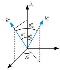
Figure 12: Illustration of the geometry in the Compton drag model showing the directions of incoming ($\hat{k}_{0}^{\prime\prime}$) and scattered ($\hat{k}_{1}^{\prime\prime}$) photons in the electron’s rest frame (ERF), which is moving with velocity $\vec{\beta}_{e}^{\prime}c$ in the comoving frame of the outflow.

4 Compton Drag

Another radiative mechanism that can yield a high degree of linear polarization is inverse-Compton scattering (ICS) of softer photons by relativistic electrons. In this model, the electrons are assumed to be cold and the bulk LF of the outflow relative to the external radiation field, that is (at least roughly) isotropic in the lab-frame, is what causes the upscattering. This mechanism has been invoked not only to explain the high level of polarization ($\Pi=80\%\pm 20\%$) that was observed in GRB 021206 (Coburn & Boggs, 2003), but also to explain the non-thermal spectrum of GRBs in general (e.g. Ghisellini & Celotti, 1999; Lazzati et al., 2000; Giannios, 2006; Lazzati & Begelman, 2006). Earlier works have discussed the potential of observing polarized emission via ICS in the context of electrons in the relativistic jet upscattering circumburst radiation fields emanating from e.g. the accretion disk (Shaviv & Dar, 1995), and in the context of a relativistic baryon-pure jet that is enveloped by slowly moving baryon-rich material. In the latter case, the shocked transition layer between the two media scatters photospheric photons and yields high levels of polarization under certain conditions (Eichler & Levinson, 2003). A proper treatment where the degree of polarization from Compton drag is obtained by averaging over the GRB image on the plane of the sky, which is different from the point source approximation adopted by earlier works, was presented by Lazzati et al. (2004).

4.1 Polarized emission due to inverse-Compton scattering: General treatment

Relativistic electrons with energies $\gamma_{e}m_{e}c^{2}$ propagating through a radiation field are slowed down by Compton scattering the soft seed photons (see for e.g. Begelman & Sikora, 1987, for a detailed exposition in the context of AGN jets). In the process, the energy of the incoming seed photon (in units of $m_{e}c^{2}$) $\varepsilon_{0}^{\prime}=E_{\gamma}^{\prime}/m_{e}c^{2}$ is increased on average to $\varepsilon_{1}^{\prime}=(4/3)\gamma_{e}^{2}\varepsilon_{0}^{\prime}$ after scattering. In the rest frame of the electron (all quantities in this frame are double-primed), the incoming photon has energy $\varepsilon_{0}^{\prime\prime}\sim\gamma_{e}\varepsilon_{0}^{\prime}$, and if $\varepsilon_{0}^{\prime\prime}\ll 1$ then the scattering is referred to as coherent or elastic and the scattering cross-section is given by the Thomson cross-section $\sigma_{T}$. In this case, $\varepsilon_{1}^{\prime\prime}=\varepsilon_{0}^{\prime\prime}$ and the scattered radiation is polarized where the degree of polarization depends on the scattering angle $\theta_{\rm sc}^{\prime\prime}=\arccos(\hat{k}_{0}^{\prime\prime}\cdot\hat{k}_{1}^{\prime\prime})$, where $\hat{k}_{0}^{\prime\prime}$ and $\hat{k}_{1}^{\prime\prime}$ are the unit wave vectors of the incoming and scattered photons, respectively (see Fig. 12). In this case, the local degree of polarization imparted to the outgoing photon is (Rybicki & Lightman, 1979)

$$\Pi^{\prime}(\theta_{\rm sc}^{\prime\prime})=\frac{1-\cos^{2}\theta_{\rm sc}^{\prime\prime}}{1+\cos^{2}\theta_{\rm sc}^{\prime\prime}}~{}.$$ (55)

In general, $\Pi^{\prime}$ is sensitive to the angle ($\theta_{0}^{\prime\prime}$) between the direction of the incoming photon and velocity vector of the electron, and the direction of the scattered photon. If the plasma is relativistically hot then the degree of polarization is obtained by integrating over all $\theta_{0}^{\prime\prime}$. For simplicity, we consider an isotropic radiation field with specific intensity $I^{\prime}_{\nu^{\prime}}(\nu^{\prime})$ through which the electron with velocity $\vec{\beta}_{e}^{\prime}c$ is propagating. In its rest frame, the electron sees an almost unidirectional radiation field with intensity

$$I^{\prime\prime}_{\nu^{\prime\prime}}(\nu^{\prime\prime})=\delta_{D,e}^{3}I^{\prime}_{\nu^{\prime}}(\nu^{\prime})\quad{\rm with}\quad\delta_{D,e}=[\gamma_{e}(1+\beta_{e}^{\prime}\mu_{0}^{\prime\prime})]^{-1}$$ (56)

where $\delta_{D,e}$ is the Doppler factor associated to the electron’s motion, $\mu_{0}^{\prime\prime}\equiv\cos\theta_{0}^{\prime\prime}$, and $\nu^{\prime\prime}=\delta_{D,e}\nu^{\prime}$. The Stokes parameters can be expressed in the same way as before, such that

$$\left\{\begin{array}[]{c}U/I\\ Q/I\end{array}\right\}=\frac{\displaystyle\int d\Omega_{0}^{\prime\prime}\delta_{D,e}^{3}I^{\prime}_{\nu^{\prime}}(\nu^{\prime\prime}/\delta_{D,e})\Pi^{\prime}(\theta_{\rm sc}^{\prime\prime})\left\{\begin{array}[]{c}\sin 2\theta_{p}^{\prime\prime}\\ \cos 2\theta_{p}^{\prime\prime}\end{array}\right\}}{\displaystyle\int d\Omega_{0}^{\prime\prime}\delta_{D,e}^{3}I^{\prime}_{\nu^{\prime}}(\nu^{\prime\prime}/\delta_{D,e})}$$ (57)

where the solid-angle $d\Omega_{0}^{\prime\prime}=d\mu_{0}^{\prime\prime}d\varphi_{0}^{\prime\prime}$. The polarization angle $\theta_{p}^{\prime\prime}$ in the electron rest frame (ERF; see Fig. 12) is obtained by first projecting the vectors $\vec{\beta}_{e}^{\prime\prime}$ and $\hat{k}_{0}^{\prime\prime}$ on the plane orthogonal to $\hat{k}_{1}^{\prime\prime}$ and then calculating the angle between the two. The scattering and polarization angles can be expressed in terms of the direction of the incoming photon ($\theta_{0}^{\prime\prime},\varphi_{0}^{\prime\prime}$) and the angle ($\theta_{1}^{\prime\prime}$) between the scattered photon and electron’s velocity vector

$$\mu_{\rm sc}^{\prime\prime} =\mu_{0}^{\prime\prime}\mu_{1}^{\prime\prime}+\sqrt{(1-{\mu_{0}^{\prime\prime}}^{2})(1-{\mu_{1}^{\prime\prime}}^{2})}\cos\varphi_{0}^{\prime\prime}$$ (58)

$$\cos\theta_{p}^{\prime\prime} =\frac{\mu_{0}^{\prime\prime}-\mu_{1}^{\prime\prime}\mu_{\rm sc}^{\prime\prime}}{\sqrt{(1-{\mu_{1}^{\prime\prime}}^{2})(1-{\mu_{\rm sc}^{\prime\prime}}^{2})}}~{},$$ (59)

where $\mu_{\rm sc}^{\prime\prime}\equiv\cos\theta_{\rm sc}^{\prime\prime}$ and $\mu_{1}^{\prime\prime}\equiv\cos\theta_{1}^{\prime\prime}$. The polarization vector is in the direction of $\hat{e}^{\prime\prime}=(\hat{k}_{0}^{\prime\prime}\times\hat{k}_{1}^{\prime\prime})/|\hat{k}_{0}^{\prime\prime}\times\hat{k}_{1}^{\prime\prime}|$, i.e. normal to the two wave vectors. The Stokes parameters calculated in the comoving frame of the outflow heretofore apply to a single electron with Lorentz factor $\gamma_{e}$. To obtain the degree of polarization in the observer frame, the Stokes parameters have to be averaged over the velocity distribution of all electrons in the emission region. When the electron velocity is ultra-relativistic ($\gamma_{e}\gg 1,~{}\beta_{e}\simeq 1$), the radiation in the electron’s rest frame is almost perfectly unidirectional and the “head-on” approximation ($\mu_{0}^{\prime\prime}=-1$) applies (Begelman & Sikora, 1987). In this case, the degree of polarization is simply given by Eq. (55) with $\theta_{\rm sc}^{\prime\prime}\to\pi-\theta_{1}^{\prime\prime}$.

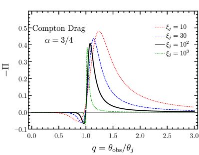
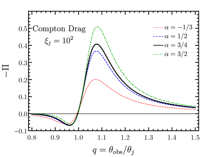
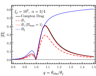
Figure 13: Degree of polarization for the Compton drag model shown as a function of viewing angle for a fixed spectral index $\alpha$ and different $\xi_{j}=(\Gamma\theta_{j})^{2}$ (top), and for different spectral indexes and fixed $\xi_{j}$ (middle). In this model, cold electrons in the comoving frame of an ultra-relativistic flow (top-hat jet with sharp edges) Thomson scatter unpolarized radiation (also see e.g. Lazzati et al., 2004; Toma et al., 2009). Also shown here (bottom) is the comparison of the degree of polarization expected in the Compton drag model to that from synchrotron radiation with $B_{\perp}$ and $B_{\parallel}$ magnetic field structures.

4.2 Polarized emission due to Compton-drag: Ultra-relativistic top-hat jet with cold electrons

If the electron distribution is cold then the electrons are moving at the bulk velocity $\vec{\beta}_{e}=\vec{\beta}\simeq 1$ in the lab-frame. In this limit, the local degree of polarization is simply given by

$$\Pi^{\prime}(\tilde{\mu}^{\prime})=\frac{1-\tilde{\mu}^{\prime 2}}{1+\tilde{\mu}^{\prime 2}}\approx\frac{2\tilde{\xi}}{1+\tilde{\xi}^{2}}~{},$$ (60)

where $\tilde{\mu}^{\prime}=\cos\tilde{\theta}^{\prime}$ and $\tilde{\theta}^{\prime}$ is the polar angle of the observed photon in the comoving frame, and the last approximate expression is obtained for $\Gamma\gg 1$, using Eq. (15) for the aberration of light. To obtain the polarization in the observer frame to which multiple fluid elements contribute, we again perform an integration over the jet geometry. Due to symmetry reasons $U=0$ and $\Pi=|Q|/I$, where

$$\frac{Q}{I}=\frac{\displaystyle\int d\tilde{\Omega}~{}\delta_{D}^{3}I^{\prime}_{\nu^{\prime}}(\nu/\delta_{D})\Pi^{\prime}(\tilde{\mu}^{\prime})\cos 2\theta_{p}}{\displaystyle\int d\tilde{\Omega}~{}\delta_{D}^{3}I^{\prime}_{\nu^{\prime}}(\nu/\delta_{D})}~{},$$ (61)

and $\theta_{p}$ is always perpendicular to the plane containing the incoming and scattered photons, which means that $\theta_{p}=\tilde{\varphi}+\pi/2$ where both $\theta_{p}$ and $\tilde{\varphi}$ are measured from the projection of the jet axis on the plane of the sky. As a result, if the jet is uniform averaging the polarization over the entire image will yield no net polarization. Therefore, the jet must be viewed off-axis to detect any polarization. We employ the same methodology here to calculate the observed degree of polarization as was used for the case of synchrotron emission due to random magnetic fields and where the jet was viewed off-axis. This can be calculated using Eq. (35, 55, 61) with $\Lambda(\tilde{\xi})=\Lambda_{C}(\tilde{\xi})$. When the incoming radiation is completely unpolarized, the intensity of the scattered radiation varies with $\tilde{\xi}$ (e.g. Rybicki & Lightman, 1979), such that

$$\Lambda_{C}=\frac{1}{2}(1+\tilde{\mu}^{\prime 2})\approx\frac{1+\tilde{\xi}^{2}}{(1+\tilde{\xi})^{2}}~{}.$$ (62)

In the following, we assume that the incoming radiation field is unpolarized, which yields

$$\Pi=\frac{\displaystyle(2\pi)^{-1}\int_{\xi_{-}}^{\xi_{+}}d\tilde{\xi}\frac{\Lambda_{C}(\tilde{\xi})}{(1+\tilde{\xi})^{2+\alpha}}\frac{2\tilde{\xi}}{1+\tilde{\xi}^{2}}\sin 2\psi(\tilde{\xi})}{\displaystyle H(1-q)\int_{0}^{\xi_{-}}d\tilde{\xi}\frac{\Lambda_{C}(\tilde{\xi})}{(1+\tilde{\xi})^{2+\alpha}}+\int_{\xi_{-}}^{\xi_{+}}d\tilde{\xi}\frac{[\pi-\psi(\tilde{\xi})]\Lambda_{C}(\tilde{\xi})}{\pi(1+\tilde{\xi})^{2+\alpha}}}~{}.$$ (63)

In the top two panels of Fig. 13, we show the degree of polarization for the Compton drag model for different viewing angles while assuming a top-hat jet. It is very similar to the corresponding polarization curves for synchrotron emission from $B_{\perp}$, with a somewhat higher normalization, corresponding $\Pi_{\rm max}\to 100\%$ for the synchrotron-$B_{\perp}$ model. This is nicely demonstrated by the dotted red line in the bottom panel of Fig. 13, which is almost on top of the curve for Compton drag (solid black line). Therefore, the degree of polarization of the synchrotron-$B_{\perp}$ model is lower than that for Compton drag by a factor of $\approx\Pi_{\rm max}=(\alpha+1)/(\alpha+5/3)\sim 0.5-0.75$. We expect the same behavior to persist also for structured jets. In particular, we expect the Compton drag polarization from a structured jet to closely follow that for the synchrotron-$B_{\perp}$ model, which is shown in the top-right panel of Fig. 9 (see also Lazzati et al., 2004), with a somewhat higher normalization, as described above.

5 Photospheric Emission

Photospheric emission from a hot and relativistically expanding fireball was first considered by Goodman (1986) and Paczyński (1986) while suggesting that GRBs are cosmological sources. The flow starts as optically thick to scattering due to copious production of $e^{\pm}$-pairs and expands adiabatically under its own pressure. Initially, the LF of the expanding fireball grows linearly with radius, $\Gamma(r)\propto r$, until all of the initial energy is transferred to the kinetic energy of the entrained baryons. Beyond this point, the fireball coasts at a constant $\Gamma$ and becomes optically thin at the photospheric radius $r=r_{\rm ph}$, where the radiation field decouples from matter. A passively expanding fireball with no energy dissipation would only give rise to a quasi-thermal spectrum (Beloborodov, 2010), which does not agree with the typical non-thermal spectrum of the prompt GRB emission. Therefore, some form of dissipation is needed in the flow, both below the photosphere and above it. Photospheric emission in dissipative jets has been considered as another alternative to synchrotron radiation in many works for the underlying mechanism of the prompt emission (e.g. Thompson, 1994; Eichler & Levinson, 2000; Mészáros & Rees, 2000; Rees & Mészáros, 2005; Lazzati, Morsony, & Begelman, 2009; Pe’er & Ryde, 2011; Bégué et al., 2013; Thompson & Gill, 2014; Gill & Thompson, 2014; Vurm & Beloborodov, 2016).

It has been shown by Beloborodov (2011, B11 hereafter) that prior to decoupling, the radiation field becomes significantly anisotropic in the comoving frame when the flow is matter dominated, such that $\rho^{\prime}c^{2}\gg U_{\gamma}^{\prime}$, where $\rho^{\prime}$ and $U_{\gamma}^{\prime}$ are the baryon rest mass density and the radiation field energy density, respectively, in the fluid’s comoving rest frame. Because of the large anisotropy, the scattered radiation becomes linearly polarized at the photosphere, in a qualitatively similar manner as in Compton drag that was discussed in the previous section. On the other hand, if the flow is radiation dominated, the angular distribution of the radiation field is preserved as the flow becomes optically thin. Since the radiation field must be isotropic in the optically thick regions, it remains so after last scattering which produces no polarization.

Here we consider a matter-dominated outflow in the form of a spherical shell expanding relativistically with bulk LF $\Gamma\gg 1$. For simplicity, we only discuss a passively expanding (non-dissipative) outflow that is carrying cold electrons (or $e^{\pm}$-pairs). We follow the treatment of B11 in writing down the spherically symmetric and frequency integrated equations of radiation transfer for the Stokes parameters in the comoving frame

$$\frac{\partial I^{\prime}}{\partial\ln r}=-(1-\mu^{\prime 2})g\frac{\partial I^{\prime}}{\partial\mu^{\prime}}-4(1-\mu^{\prime}g)I^{\prime}+\tau_{T}\frac{(S^{\prime}-I^{\prime})}{1+\mu^{\prime}}~{},$$ (64)

$$\frac{\partial Q^{\prime}}{\partial\ln r}=-(1-\mu^{\prime 2})g\frac{\partial Q^{\prime}}{\partial\mu^{\prime}}-4(1-\mu^{\prime}g)Q^{\prime}+\tau_{T}\frac{(R^{\prime}-Q^{\prime})}{1+\mu^{\prime}}~{},\quad\quad$$ (65)

where the degree of polarization is given by $\Pi=|Q^{\prime}|/I^{\prime}$. In the above equation, $S^{\prime}$ and $R^{\prime}$ are the source functions (Chandrasekhar, 1960; Sobolev, 1963)

$$S^{\prime}(\mu^{\prime},r)=I^{\prime}_{0}+\frac{3}{8}(3\mu^{\prime 2}-1)\left(I_{2}^{\prime}-\frac{I^{\prime}_{0}}{3}+Q^{\prime}_{0}-Q^{\prime}_{2}\right)$$ (66)

$$R^{\prime}(\mu^{\prime},r)=\frac{9}{8}(1-\mu^{\prime 2})\left(I_{2}^{\prime}-\frac{I_{0}^{\prime}}{3}+Q_{0}^{\prime}-Q_{2}^{\prime}\right)~{},$$ (67)

where

$$\{I_{m}^{\prime}(r)~{},~{}Q_{m}^{\prime}(r)\}=\frac{1}{2}\int_{-1}^{1}\{I^{\prime}(\mu^{\prime},r)~{},~{}Q^{\prime}(\mu^{\prime},r)\}\mu^{\prime m}d\mu^{\prime}$$ (68)

are the moments of total and polarized intensities. The quantity

$$g(r)=1-\frac{d\ln\Gamma(r)}{d\ln r}$$ (69)

expresses the acceleration profile of the flow; for a coasting flow $g=1$. In this case, the Thomson optical depth of a relativistically expanding outflow along a radial trajectory is (Abramowicz, Novikov, & Paczyński, 1991)

$$\tau_{T}(r)=\int_{r}^{\infty}n_{e}^{\prime}(r)\sigma_{T}\Gamma(1-\beta)dr=\frac{n_{e}^{\prime}(r)\sigma_{T}r}{2\Gamma}.$$ (70)

The comoving volume of the outflow scales as $V^{\prime}=4\pi r^{2}\Delta^{\prime}\propto r^{2}$, where it has comoving width $\Delta^{\prime}$. As a result, the number density of electrons scales as $n_{e}^{\prime}\propto r^{-2}$ and therefore $\tau_{T}(r)\propto r^{-1}$. At the photospheric radius $\tau_{T}(r_{\rm ph})\equiv 1$ and the Thomson optical depth can simply be expressed as

$$\tau_{T}(r)=\frac{r_{\rm ph}}{r}~{}.$$ (71)

Deeper in the flow, at $r\ll r_{\rm ph}$ where $\tau_{T}\gg 1$, matter and radiation are tightly coupled via Compton scattering that causes the radiation field to be isotropic. The flow expands adiabatically under its own pressure where the radiation field loses energy to $PdV$ work, such that the comoving intensity declines over radius as

$$I^{\prime}(r)=I^{\prime}_{\rm ph}\left(\frac{r}{r_{\rm ph}}\right)^{-8/3}~{},$$ (72)

where $I_{\rm ph}^{\prime}$ is the normalization of the intensity at the photosphere. The above equation is strictly valid at $\tau_{T}\gtrsim 10$ and it begins to break down near the photosphere where the radiation field becomes highly anisotropic (B11). However, the difference is of order unity, and therefore we will assume that the adiabatic cooling of the radiation field approximately applies all the way up to the photosphere.

The total isotropic equivalent power carried by the outflow is $L_{\rm tot,iso}=L_{\gamma,{\rm iso}}+L_{\rm k,iso}$, where $L_{\rm k,iso}$ is the kinetic power of the baryons and $L_{\gamma,{\rm iso}}$ is the luminosity of the radiation field which is given by

$$L_{\gamma,{\rm iso}}(r)=4\pi r^{2}F=4\pi r^{2}\int I(\mu,r)\mu d\Omega=16\pi^{2}r^{2}I_{1}~{}.$$ (73)

The first moment of the lab-frame intensity $I_{1}$ can be expressed in terms of the comoving-frame quantities via Lorentz transformation, which gives (B11)

$$I_{1}=\Gamma^{2}[\beta(I_{0}^{\prime}+I_{2}^{\prime})+(1+\beta^{2})I_{1}^{\prime}]\approx\frac{4}{3}\Gamma^{2}\beta I^{\prime}~{}.$$ (74)

Depending on the amount of baryons carried by the flow $\Gamma(r)$ saturates at $r=r_{s}=\eta r_{0}$, where $\eta=L/\dot{M}_{b}c^{2}$ is the total energy per unit rest energy, $\dot{M}_{b}$ is the mass flux of baryons, $L$ is the total jet power, and $r_{0}$ is the radius at which the flow was launched. For $r>r_{s}$ the radiation field provides no acceleration and the flow simply coasts at a constant $\Gamma=\eta$. At this point, the enthalpy density of the radiation field equals that of matter, $4e_{\gamma}^{\prime}/3=e_{m}^{\prime}+p_{m}^{\prime}$. Here, $e_{\gamma}^{\prime}$ and $e_{m}^{\prime}$ are the comoving energy densities of the radiation field and matter (including its rest mass energy), respectively, and $p^{\prime}_{m}$ is the thermal pressure of the matter component. This also implies that $L_{\gamma,{\rm iso}}(r_{s})=L_{\rm k,iso}(r_{s})=(1/2)L_{\rm tot,iso}$, which by combining Eq.(72,73,74) yields the powers measured by an observer at $r=\infty$ for the two components,

$$L_{\gamma,{\rm iso},\infty} \approx \frac{64\pi^{2}}{3}r_{\rm ph}^{2}\Gamma^{2}\beta I^{\prime}_{\rm ph}$$ (75)

$$L_{\rm k,iso,\infty} \approx \left(\frac{r_{\rm ph}}{r_{s}}\right)^{2/3}L_{\gamma,{\rm iso},\infty}\approx\epsilon_{\gamma}^{-1}L_{\gamma,{\rm iso},\infty}~{},$$ (76)

where the adiabatic factor is defined as

$$\epsilon_{\gamma}\equiv\frac{L_{\gamma,{\rm iso},\infty}}{L_{\gamma,{\rm iso}}+L_{\rm k,iso}}\approx\frac{L_{\gamma,{\rm iso},\infty}}{L_{{\rm k,iso},\infty}}\approx\left(\frac{r_{\rm ph}}{r_{s}}\right)^{-2/3}$$ (77)

The isotropic power carried by a passively expanding cold flow, for which $e_{m}^{\prime}=n_{e}^{\prime}m_{p}c^{2}$ and $p_{m}^{\prime}=0$, is given by

$$L_{k,\rm iso}(r)=4\pi r^{2}\Gamma^{2}\beta n_{e}^{\prime}m_{p}c^{3}\approx 4\pi r^{2}\Gamma^{2}n_{e}^{\prime}m_{p}c^{3}~{},$$ (78)

where $m_{p}$ is the proton mass and $n_{e}^{\prime}$ is the density of the baryonic electrons. From the expression for the Thomson optical depth in Eq. (70), we find that the photospheric radius for this outflow is

$$r_{\rm ph}=\frac{\sigma_{T}L_{\rm k,iso}}{8\pi\Gamma^{3}c^{3}m_{p}}\approx 5.5\times 10^{12}\Gamma_{2}^{-3}L_{\rm k,iso,52}~{}{\rm cm}~{}.$$ (79)

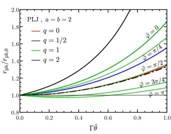
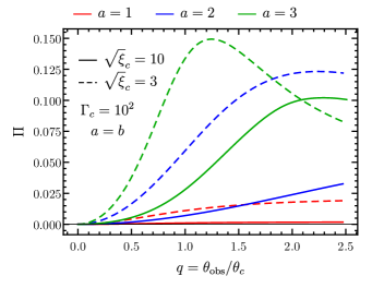
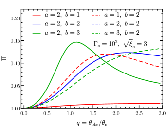
Figure 14: Top: Deviation of the photospheric radius within the beaming cone with respect to that obtained along the LOS, shown here for different values of $q\equiv\theta_{\rm obs}/\theta_{c}$. The change in $r_{\rm ph}$ with azimuthal angle is shown here for $q=1$ and different values of $\tilde{\varphi}$ as green dotted lines. The black dash-dotted line shows the result for a spherical flow with no angular structure. Here we assumed $\Gamma_{c}=10^{3}$ and $\xi_{c}\equiv(\Gamma_{c}\theta_{c})^{2}=10^{2}$. Middle: Degree of polarization arising from photospheric emission in a power law jet (PLJ), shown for a narrow ($\sqrt{\xi}_{c}=3$) and wide ($\sqrt{\xi}_{c}=10$) jet. Bottom: The polarization trend for different values of the power law indices ($a,b$) is shown.

5.1 $\Pi$ from a structured jet viewed off-axis

To obtain the observed polarization, integration over the GRB image must be performed. An important consequence of this integration is that radiation emerging from within the beaming cone (of angular size $\Gamma^{-1}$) experiences different Thomson optical depths, such that $\tau_{T}=\tau_{T}(\tilde{\theta},\tilde{\varphi})$. Therefore, the matter-radiation decoupling radius also varies with angle around the LOS, $r_{\rm ph}=r_{\rm ph}(\tilde{\theta},\tilde{\varphi})$, which leads to variations in $\Pi=\Pi(\tilde{\theta},\tilde{\varphi})$ around the LOS. If the properties of the flow are symmetric around the LOS, the observed polarization vanishes (similarly to Compton drag or synchrotron for $B_{\perp}$ or $B_{\parallel}$, in which there is symmetry around the local radial direction). Therefore, the outflow must either be structured or the intensity must be inhomogeneous.

In general, due to the statistical nature of last scattering, the photospheric radius is a random variable (B11). As a consequence, the matter-radiation decoupling doesn’t occur at a sharp boundary, but instead it is radially extended where roughly $2/3$ of the photons undergo last scattering at $r_{\rm ph}/3<r<3r_{\rm ph}$. This leads to the notion of a “fuzzy” photosphere (B11). For simplicity, here we adopt the sharp photosphere.

In the following we consider a power-law structured jet that was as discussed earlier. The Thomson optical depth measured in the direction of the observer ($\hat{n}$) around the LOS along some photon trajectory $\mathcal{S}$, with length $s=r\cos\tilde{\theta}=\tilde{z}$, is

$$\tau_{T}=\int n_{e}^{\prime}(r,\theta)\sigma_{T}ds^{\prime}=\int_{\tilde{z}}^{\infty}n_{e}^{\prime}(r,\theta)\sigma_{T}\Gamma(\theta)[1-\beta(\theta)\tilde{\mu}]ds~{},$$ (80)

where we made use of the fact that $ds=\delta_{D}ds^{\prime}$. For $\tilde{\mu}=1$, one recovers the expression in Eq. (70). The transverse distance from the LOS to the path $\mathcal{S}$ is a constant, such that $r\sin\tilde{\theta}=r_{\rm ph}\sin\tilde{\theta}_{\rm ph}$, which results from the fact that light travels in a straight path. This can be used to write the integral over the more useful quantity $\tilde{\theta}$ instead of $s$ through the Jacobian of transformation

$$ds=\frac{ds}{d\tilde{\theta}}d\tilde{\theta}=-\frac{r^{2}}{r_{\rm ph}\sin\tilde{\theta}_{\rm ph}}d\tilde{\theta}~{}.$$ (81)

Finally, by noticing that $\tau_{T}=1$ at the photospheric radius, we find

$$r_{\rm ph}(\tilde{\theta},\tilde{\varphi})=\frac{\sigma_{T}}{\sin\tilde{\theta}}\int_{0}^{\tilde{\theta}}n^{\prime}_{e}(r,\theta)r^{2}\Gamma(\theta)[1-\beta(\theta)\tilde{\mu}^{\prime\prime}]d\tilde{\theta}^{\prime\prime}~{},$$ (82)

where $\tilde{\theta}^{\prime\prime}$ is a dummy variable, and $\theta=\arccos\mu$ can be expressed in terms of the LOS coordinates ($\tilde{\theta},\tilde{\varphi}$) using

$$\mu=\tilde{\mu}\tilde{\mu}_{\rm obs}-\cos\tilde{\varphi}\sqrt{(1-\tilde{\mu}^{2})(1-\tilde{\mu}_{\rm obs}^{2})}~{}.$$ (83)

For an ultra-relativistic structured jet, the isotropic equivalent kinetic power is

$$L_{k,{\rm iso}}(\theta)=4\pi r^{2}\Gamma^{2}(\theta)n^{\prime}_{e}(r,\theta)m_{p}c^{3}~{}.$$ (84)

From here it is easy to see that

$$r^{2}n^{\prime}_{e}(r,\theta)\equiv\hat{n}_{e}^{\prime}(\theta)\propto\frac{L_{k,{\rm iso}}(\theta)}{\Gamma^{2}(\theta)}\approx\frac{L_{\rm tot,iso}(\theta)}{\Gamma^{2}(\theta)}$$ (85)

is a completely $r$ independent quantity and it only varies with polar angle $\theta$. Then, along the LOS, for which $\theta=\theta_{\rm obs}$ and $\tilde{\theta}=0$, the photospheric radius lies at

$$r_{\rm ph,0}=\frac{\sigma_{T}\hat{n}_{e}^{\prime}(\theta_{\rm obs})}{2\Gamma(\theta_{\rm obs})}~{}.$$ (86)

The deviation of the photospheric radius along photon trajectories that originate at different $\tilde{\theta}$ and $\tilde{\varphi}$ around the LOS is shown in the top panel of Fig. 14.

The comoving intensity will also be modified due to the angular structure of the outflow. Its angular dependence can be obtained by expressing the normalization $I^{\prime}_{\rm ph}$ in terms of $L_{\rm k,iso,\infty}(\theta)$ and $\Gamma(\theta)$ from Eq.(76 & 79), such that

$$I^{\prime}_{\rm ph}(\theta)\propto\frac{\Gamma(\theta)^{20/3}}{L_{\rm k,iso}^{5/3}(\theta)}\equiv\kappa(\theta)~{}.$$ (87)

The flux measured by a distant observer is given by

$$F=\frac{1}{d_{L}^{2}}\int\delta_{D}^{4}I^{\prime}(r)dS_{\perp}=\frac{1}{d_{L}^{2}}\int\delta_{D}^{4}I^{\prime}(r)\tilde{\rho}d\tilde{\rho}d\tilde{\varphi}~{},$$ (88)

where $dS_{\perp}$ is the differential area on the plane of the sky and $\tilde{\rho}=r_{\rm ph}\sin\tilde{\theta}_{\rm ph}$ is the transverse distance from the LOS. For convenience, the above integral can be performed over the polar angle $\tilde{\theta}$ via a simple transformation,

$$d\tilde{\rho}=\frac{d\tilde{\rho}}{d\tilde{\theta}}d\tilde{\theta}=r_{\rm ph}\tilde{\mu}\left(1+\frac{\sqrt{1-\tilde{\mu}^{2}}}{\tilde{\mu}}\frac{d\ln r_{\rm ph}}{d\tilde{\theta}}\right)d\tilde{\theta}~{},$$ (89)

which finally yields,

$$dS_{\perp}=r_{\rm ph}^{2}\left(\tilde{\mu}+\sqrt{1-\tilde{\mu}^{2}}\frac{d\ln r_{\rm ph}}{d\tilde{\theta}}\right)d\tilde{\mu}d\tilde{\varphi}~{}.$$ (90)

Now, the degree of polarization measured by a distant observer can be expressed as

$$\Pi=\frac{Q}{I}=\frac{\displaystyle\int\delta_{D}^{4}Q^{\prime}(r_{\rm ph})\kappa(\theta)\cos(2\tilde{\varphi})dS_{\perp}}{\displaystyle\int\delta_{D}^{4}I^{\prime}(r_{\rm ph})\kappa(\theta)dS_{\perp}}~{},$$ (91)

where $I^{\prime}(r_{\rm ph})$ and $Q^{\prime}(r_{\rm ph})$ are obtained from the radiative transfer equations for a spherically symmetric flow, with the angular structure embedded in $\kappa(\tilde{\theta},\tilde{\varphi})$ and $r_{\rm ph}(\tilde{\theta},\tilde{\varphi})$.

To be able to use the radiative transfer solutions from Eq. (LABEL:eq:Iprime & 65) that assume a spherical outflow, to calculate the degree of polarization when the outflow has an angular structure, an important consideration is choosing the correct angular scale $\Delta\theta$ over which the properties of the outflow don’t change significantly. The properties of the flow change significantly over angular scales $\delta\theta_{\epsilon}$, where the fractional change in the energy per unit solid angle of the outflow is of order unity, such that $\Delta\epsilon/\epsilon\sim 1$ (similar considerations also apply for the angular dependence of $\Gamma$). Therefore, the spherically symmetric solution to the radiative transfer equations is approximately valid on angular scales

$$\Delta\theta\ll\delta\theta_{\epsilon}\equiv\theta\left|\frac{d\ln\epsilon}{d\ln\theta}\right|^{-1}~{}.$$ (92)

For a structured jet with a uniform core and power-law wings, the energy per unit solid angle is $\epsilon(\theta)\propto\theta^{-a}$ outside of the core, which yields $\delta\theta_{\epsilon}=\max[\theta_{c},\theta/a]$.

Next, we compare the angular scale $\Delta\theta$ with the typical angular scale over which photons are scattered $\tilde{\theta}_{\rm sc}$ while they try to diffuse from deep within the flow outwards. In the comoving frame, their diffusion length can be expressed as $\ell^{\prime}_{\rm diff}\sim\sqrt{N_{\rm sc}}\lambda^{\prime}$, where $N_{\rm sc}$ is the mean number of scatterings they undergo and $\lambda^{\prime}$ is their mean free path. In a relativistically expanding flow, $N_{\rm sc}\sim\tau_{T}$ rather than $\tau_{T}^{2}$, where the Thomson optical depth of the flow is $\tau_{T}=r/(\Gamma\lambda^{\prime})$. This finally yields the diffusion length of photons $\ell^{\prime}_{\rm diff}\sim r/(\Gamma\sqrt{\tau_{T}})$, which suggests that deeper in the flow, where $\tau_{T}\gg 1$, photons only diffuse a very short distance and are instead advected with the flow. If the photons diffuse a mean transverse distance $r\sin\tilde{\theta}_{\rm sc}\sim r\tilde{\theta}_{\rm sc}$ of the order of the diffusion distance, such that $r\tilde{\theta}_{\rm sc}\sim\ell^{\prime}_{\rm diff}$, then the mean scattering angle is $\tilde{\theta}_{\rm sc}\sim(\Gamma\sqrt{\tau_{T}})^{-1}$. Finally, letting $\Delta\theta=\tilde{\theta}_{\rm sc}$, yields the constraint

$$\Gamma\theta\gg\frac{a}{\sqrt{\tau_{T}}}~{}.$$ (93)

In a structured jet, outside of the uniform core that has angular size $\theta_{c}$, the LF decays with angle $\theta$ away from the jet symmetry axis (see Eq.(50)). For $\theta>\theta_{c}$, $\Gamma\theta\sim\Gamma_{c}\theta_{c}(\theta/\theta_{c})^{1-b}$, where $\Gamma_{c}\theta_{c}\sim 3-10$ and $\Gamma_{c}\gg 1$. In this case, deeper in the flow the above condition is almost always satisfied, however, close to the photosphere, where $\tau_{T}\sim 1$, it breaks down for $b>1$ beyond some critical angle. This is one caveat of the approximation made here. However, $\Gamma\theta<1$ implies lateral causal contact, for which the flow dynamics naturally tend to wash out lateral gradiants.

In the middle and bottom panels of Fig. 14, we show the degree of polarization of photospheric emission when the outflow is structured with having a power law jet (PLJ; Eq. 49) profile. In this case, when the bulk LF falls sharply outside of the narrow core for a given profile of the kinetic power, we find a moderate level of polarization with $\Pi\lesssim 15\%$ for narrow jets ($\sqrt{\xi}_{c}=3$) and $\Pi\lesssim 10\%$ for wider jets ($\sqrt{\xi}_{c}=10$). This result is broadly consistent with that found from Monte Carlo simulations of photospheric emission from structured jets (Ito et al., 2014; Lundman, Pe’er, & Ryde, 2014), where it was found that $\Pi\sim 20\%-30\%$ when $\xi_{c}\sim 10$ and $\Pi\lesssim 20\%$ when $\xi_{c}\sim 10^{2}$. The exact result depends on the angular structure assumed in such simulations. Looking at the trend of $\Pi$ as the power law indices of the $\Gamma(\theta)$ and $L_{k,\rm iso}(\theta)$ profiles are changed, it is clear from the bottom panel of Fig. 14 that a steeper $\Gamma(\theta)$ profile yields higher degree of polarization. On the other hand, steeper kinetic power profiles only translate the polarization curve to larger $q$ values while approximately maintaining the same maximum level of $\Pi$.

6 Integration over multiple pulses

Unless the source is nearby or particularly bright, observations of the prompt phase in GRBs are typically photon starved. To increase photon statistics observers generally have to average over multiple pulses, which washes out any temporal dependence. This is especially true for polarization measurements. On the one hand, this may be the only way to derive a statistically significant measurement of the level of polarization, while on the other hand this operation guarantees the loss of crucial information such as the temporal dependence of the polarization angle. More importantly, since the properties of the outflow, e.g. $\Gamma$ or equivalently $\xi_{j}$ for a fixed $\theta_{j}$, can also change from pulse to pulse, this can affect the level of polarization when integrating over multiple pulses.

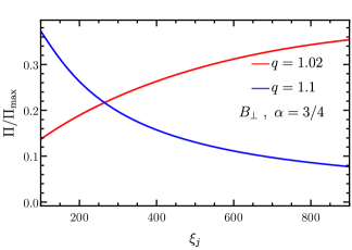
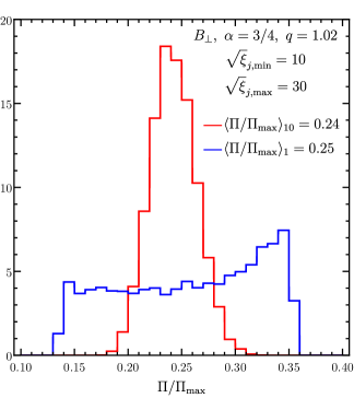
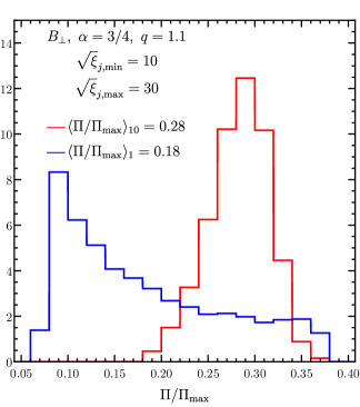
Figure 15: Top: The trend of $\Pi$, either monotonically decaying ($q=\theta_{\rm obs}/\theta_{j}=1.1$) or rising ($q=1.02$), as $\xi_{j}=(\Gamma\theta_{j})^{2}$ of the individual pulses is varied. Shown here for the case of a random magnetic field completely in the plane of the ejecta. The chosen values of $q$ are not special, but yield high levels of polarization in this particular case. Middle & Bottom: Distribution of $\Pi$ when obtained from a single pulse (blue) or after having integrated over multiple pulses (red; $N_{p}=10$) in an emission episode. Shown here for two different values of $q$ for which the trend of $\Pi$ is opposite when $\xi_{j}^{1/2}$ is varied between pulses. Here $\xi_{j,\min}^{1/2}\leq\xi_{j}^{1/2}\leq\xi_{j,\max}^{1/2}$ is distributed uniformly.

The total polarization of an emission episode, which is a sum of $N_{p}>1$ pulses, is obtained from summing up their respective Stokes parameters,

$$\Pi=\frac{Q}{I}=\frac{\sum_{i=1}^{N_{p}}Q_{i}}{\sum_{i=1}^{N_{p}}I_{i}}~{}.$$ (94)

In the case of an ordered magnetic field with coherence length as large as the size of the emission region that produces a single pulse, multiple pulses arising from such mutually incoherent patches will yield a lower degree of polarization. This occurs due to the fact that the PAs of emission from different patches are randomly oriented which leads to cancellations and leave a lower level of net polarization. Adding up the polarization from $N_{p}$ pulses is essentially a random walk for $Q$ while $I$ adds up coherently. Therefore, the total polarization for $N_{p}$ pulses can be deduced from the above equation to obtain (Gruzinov & Waxman, 1999)

$$\Pi\sim\frac{\Pi_{\max}}{\sqrt{N_{p}}}~{}.$$ (95)

For other magnetic field configurations, cancellation of polarization between different pulses due to the change of sign of $\Pi_{i}=Q_{i}/I_{i}$ (i.e. of $Q_{i}$, since $I_{i}>0$) may not occur.

6.1 Distribution of $\Pi$ in a single burst

Here we consider a single burst and an emission episode with an agglomeration of multiple pulses that may be produced by emission regions with different $\Gamma$. The distribution of $\Gamma$ in the different pulses that correspond to different emission regions is not known, and assumed to be drawn from some probability distribution over a finite range $\Gamma_{\min}\leq\Gamma\leq\Gamma_{\max}$. For simplicity we assume here that $\theta_{j}$, and therefore also $q=\theta_{\rm obs}/\theta_{j}$, remains fixed over the entire GRB. Therefore, a distribution of $\Gamma$ is equivalent to that of $\xi_{j,\min}^{1/2}\leq\xi_{j}^{1/2}\leq\xi_{j,\max}^{1/2}$. In what follows, we consider a uniform distribution of $\xi_{j}^{1/2}$, such that $P\left(\xi_{j}^{1/2}\right)=\left(\xi_{j,\max}^{1/2}-\xi_{j,\min}^{1/2}\right)^{-1}$. The following analysis can be easily extended to other distributions, however, there’s no straightforward way of discerning one from the other. To demonstrate the effect of averaging over multiple pulses, for simplicity, we will consider in this section a top-hat jet with a random magnetic field ($B_{\perp}$) in the plane of the ejecta. We carry out a Monte-Carlo (MC) simulation where we draw $10^{4}$ random samples, where each sample represents an emission episode with $N_{p}$ pulses.

On average integration over multiple pulses can yield $\Pi$ that is higher or lower in comparison to a single pulse. This depends on the viewing angle, in particular $q$, and the trend of $\Pi$ as $\xi_{j}$ is varied (see top panel of Fig. 15). We illustrate this with two cases, as shown in the middle and bottom panel of Fig. 15, where the value of $q$ is chosen so that the trend of $\Pi$ is opposite. Since the jet is fairly wide with $\xi_{j}>10^{2}$, there is no cancellation of the polarization as $\Pi_{i}$ never switches sign in this case. However, for narrower jets with $\xi_{j}<10$ multiple pulses with even smaller $\xi_{j}$ and $q\lesssim 1$ can have opposite signs for the PA leading to cancellation and lower net polarization.

7 Statistical inference of magnetic field structure from polarization

A firm detection of linear polarization can provide valuable insight into the structure of the magnetic field in the outflow, which can be further used to constrain the jet composition. In order to derive meaningful inference about the magnetic field structure from the measured degree of polarization, there are three basic quantities that determine the outcome: (i) $\xi_{j}^{1/2}=\Gamma\theta_{j}$, which determines how narrow the jet is and varies between different pulses due to variation in $\Gamma$ while $\theta_{j}$ is assumed here to be fixed for a given burst; (ii) $q=\theta_{\rm obs}/\theta_{j}$, which determines the viewing angle and remains fixed for the different pulses but varies between different bursts; and (iii) $\tilde{f}_{\rm iso}(q,\xi_{j})\equiv E_{\gamma,{\rm iso}}(q,\xi_{j})/E_{\gamma,{\rm iso}}(0,\xi_{j})$ or equivalently the off-axis to on-axis fluence ratio, which depends on both $\xi_{j}$ and $q$ and varies between bursts as well as different pulses. The appropriate relative weight ($E_{\gamma,{\rm iso}}$) is assigned to each pulse when adding up the Stokes parameters for different pulses that are added up in order to increase the observed signal.

Additional effects that characterize the spectrum, viz. the $\nu F_{\nu}$-peak energy and the spectral indices above and below it, can also have an effect (see, e.g., Toma et al., 2009). For instance, if the spectral peak is located in a given frequency band, $\nu_{1}<\nu_{\rm pk}<\nu_{2}$, then its temporal evolution will be reflected in the temporal evolution of the polarization. As it was shown earlier, the degree of polarization depends on the spectral index in both synchrotron and Compton drag emission mechanisms, where softer spectra yield a larger degree of polarization. Therefore, dominance of a given spectral component is reflected in the corresponding level of polarization, making this spectro-polarimetric correlation a useful probe of the underlying emission mechanism. The evolution of the spectral properties over multiple pulses is not considered in this work to limit the degrees of freedom, and therefore to ensure the robustness of the results. The formalism developed in this work can be easily extended to include spectral and temporal effects.

For simplicity we consider a fixed initial jet opening angle $\theta_{j}$. This renders the distribution of the three basic parameters to arise due to the spread in the viewing angle $\theta_{\rm obs}$ between different GRBs and of $\Gamma$ also between different pulses within the same GRB. First we consider a uniform distribution of $\Gamma$ or equivalently of $\xi_{\{j,c\},\min}^{1/2}\leq\xi_{\{j,c\}}^{1/2}\leq\xi_{\{j,c\},\max}^{1/2}$, where the subscript $j$ applies when discussing a top-hat jet with sharp or smooth edges, and the subscript $c$ applies when discussing a structured jet with a compact core. For brevity, only the subscript $j$ is used in the following discussion. The viewing angle is distributed according to the solid angle, such that $P(\theta_{\rm obs})d\theta_{\rm obs}=\sin\theta_{\rm obs}d\theta_{\rm obs}$. Finally, the off-axis to on-axis fluence ratio depends on the distribution of $\xi_{j}$ and $q$. These are obtained for a fixed $\theta_{j}$, such that $P(\xi_{j})d\xi_{j}=P\left(\xi_{j}^{1/2}\right)d\xi_{j}^{1/2}$ and $P(q)dq=P(\theta_{\rm obs})d\theta_{\rm obs}$, which yields

$$P(\xi_{j})=\frac{P\left(\xi_{j}^{1/2}\right)}{2\xi_{j}^{1/2}}$$ (96)

$$P(q)=\theta_{j}P(\theta_{\rm obs})\propto q~{}.$$ (97)

Since $P(q)\propto q$, it would favour larger $q>1$ values, for which the fluence will be too small. Therefore, a more meaningful distribution of $q$ should account for the rapid drop in fluence for $q>1$. To include this effect, we define a fluence weighted distribution for $q$ with $\bar{P}(q)=[\int\bar{f}_{\rm iso}(q)P(q)dq]^{-1}\bar{f}_{\rm iso}(q)P(q)$, where

$$\bar{f}_{\rm iso}(q)=\int_{\xi_{j,{\min}}}^{\xi_{j,{\max}}}\tilde{f}_{\rm iso}(q,\xi_{j})P(\xi_{j})d\xi_{j}$$ (98)

is the distribution of $\tilde{f}_{\rm iso}(q,\xi_{j})$ with $q$ but marginalized over the distribution of $\xi_{j}$. Fig. 16 shows the fluence weighted distribution of $\bar{P}(q)$ for two different jet opening angles and for a uniform distribution in $\sqrt{\xi}_{j}$. The suppression in $\bar{P}(q)$ for $q\gtrsim 1$ is caused by the sharp (gradual) drop in fluence for a top-hat (structured) jet. This has important implications for the distribution of detected GRBs since for flux limited detectors the drop in fluence reduces the effective volume probed by the detector. For a top-hat jet the drop in fluence is so sharp that the total number of GRBs in a given volume can be obtained from $N_{\rm tot}=f_{b}N_{\rm obs}$, where $f_{b}=4\pi/\Delta\Omega=4\pi/(1-\cos\theta_{j})\approx 4/\theta_{j}^{2}$ is the beaming factor for $\theta_{j}\ll 1$. However, for a structured jet, this estimate must take into account the dependence on $q$.

To simulate different bursts we carried out MC simulations with $10^{4}$ sample bursts and $N_{p}=10$ multiple pulses for each burst. For each sample burst, a value of $q$ was randomly drawn from $\bar{P}(q)$ and for each pulse the distribution of $\xi_{j}^{1/2}$ was randomly sampled. To further eliminate the polarization contribution from pulses with low fluence, only pulses with $\tilde{f}_{\rm iso}(q,\xi_{j})>10^{-2}$ were included. This threshold implies that the detectors are flux limited and can only detect bursts/pulses that are dimmer by a factor of $10^{-2}$ from their absolute on-axis fluence. Since dimmer pulses would fall below the detector threshold and won’t be detected, their contribution to $\Pi$ should be removed when calculating the total polarization. Here we don’t take into account the limitation imposed by the compactness of the flow for even modestly steep $\Gamma(\theta)$ profiles. Such a constraint would restrict viewing angles to even smaller values as compared to the constraint on $q$ imposed by $\tilde{f}_{\rm iso}$. In order to incorporate this effect, more detailed spectral modeling than conducted in this work would be needed which is outside the scope of this work.

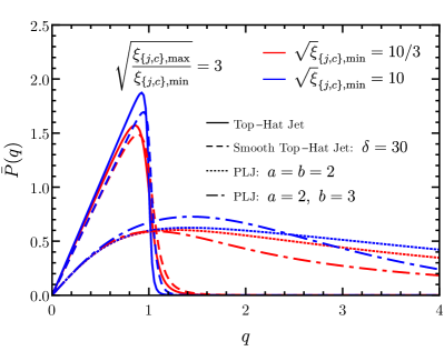
Figure 16: Fluence weighted distribution of $q=\theta_{\rm obs}/\theta_{j}$ that is marginalized over a uniform distribution of $\sqrt{\xi}_{\{j,c\},\min}\leq\sqrt{\xi}_{\{j,c\}}\leq\sqrt{\xi}_{\{j,c\},\max}$. Shown here for four different jet structures.

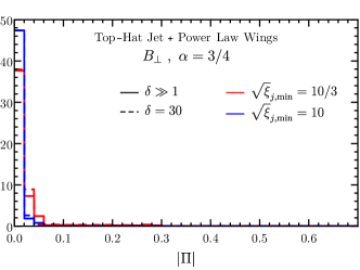
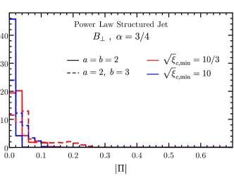
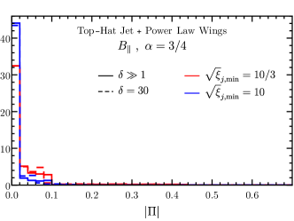
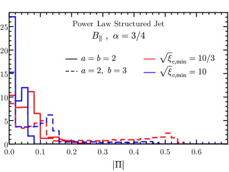
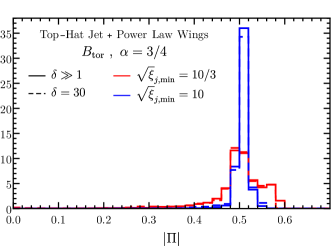
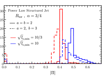
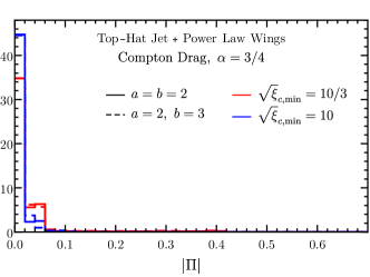
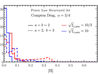
Figure 17: Distribution of $|\Pi|$ arising from synchrotron radiation and Compton drag when integrated over multiple ($N_{p}=10$) pulses for different magnetic field configurations and jet structures, with spectral index $\alpha=3/4$. The total sample consists of $10^{4}$ simulated GRBs with fluence weighted distribution of $q=\theta_{\rm obs}/\theta_{j}$ or $q=\theta_{\rm obs}/\theta_{c}$. For each burst, the multiple pulses are randomly sampled from a uniform distribution of $\sqrt{\xi}_{\{j,c\},\min}\leq\sqrt{\xi}_{\{j,c\}}\leq\sqrt{\xi}_{\{j,c\},\max}$, with $\sqrt{\xi}_{\{j,c\},\max}=3\sqrt{\xi}_{\{j,c\},\min}$.

In Fig. 17 we show the distribution of $|\Pi|$ arising from Compton drag and from synchrotron emission for different configurations of the magnetic field and different jet geometries. It is clear that only a globally ordered field, such as a toroidal field, can yield high levels of polarization. Any random field component ($B_{\perp}$) or a locally ordered ($B_{\parallel}$) field will statistically most likely produce $\Pi\lesssim 5\%-10\%$ only if the jet is structured with moderately sharp gradients in $\Gamma$. For a top-hat jet both field configurations yield $\Pi\lesssim 1\%$. The same is true for the case of Compton drag. Broadly similar results were obtained by Pearce et al. (2019).

Since the true distribution of $\Gamma$ is unclear, we have tested the robustness of the results shown in Fig. 17 by using two additional distributions of $\xi_{j}^{1/2}$: (i) a uniform distribution in $\ln\xi_{j}^{1/2}$, and (ii) a log-normal distribution, which are expressed as the following

$$(i)\quad\quad P(\ln\xi_{j}^{1/2})=\left[\ln\left(\frac{\xi_{j,\max}^{1/2}}{\xi_{j,\min}^{1/2}}\right)\right]^{-1}$$ (99)

$$(ii)\quad\quad P(\xi_{j}^{1/2})=\frac{1}{\xi_{j}^{1/2}\sigma\sqrt{2\pi}}\exp\left[-\frac{(\ln\xi_{j}^{1/2}-\mu)^{2}}{2\sigma^{2}}\right]~{},$$ (100)

where $\mu$ and $\sigma$ are the mean and standard deviation, respectively, of the distribution which results after taking the natural logarithm of the log-normally distributed $\xi_{j}^{1/2}$. In a population synthesis study carried out by Ghirlanda et al. (2013) using a large sample of Swift/BAT, Fermi/GBM and CGRO/BATSE GRBs, it was found that the distribution of $\Gamma$ is best represented by a log-normal distribution with $\mu_{\Gamma}\sim 4.5$ and $\sigma_{\Gamma}\sim 1.5$. This result was obtained under the assumption that both the $(\nu F_{\nu})$-peak and true jet energies in the comoving frame are clustered around typical values in a large sample of GRBs. In addition, it was assumed that the product $\theta_{j}^{2.5}\Gamma=\,$const. Here we assume the same underlying distribution of $\Gamma$ with ($\mu_{\Gamma},\sigma_{\Gamma}$), and also assume a fixed $\theta_{j}=10^{-1}$ in order to switch from $P(\Gamma)$ to $P(\xi_{j}^{1/2})$.

In the left panel of Fig. 18, we compare the results of the three distributions when the magnetic field configuration is given by $B_{\rm tor}$ and the outflow has a power law angular structure. We find that all three distributions of $\xi_{c}^{1/2}$ produce very similar predictions for $|\Pi|$ with a small spread ($<10\%$) which shows that the results are quite robust. In the right panel, we compare the predictions of the synchrotron model to measurements of polarization in the prompt emission of GRBs that have at least $3\sigma$ detection significance. Apart from a small variation introduced by different spectral indices $\alpha$ in the given bursts in the model distributions, the measured high degree of polarization appear to favour a globally ordered toroidal field configuration of the outflow magnetic field.

In the right panel of Fig. 18, we compare the degree of polarization expected from a power law structured jet, when the prompt $\gamma$-ray emission mechanism is either synchrotron or Compton drag, to statistically significant measurements and upper limits of $\Pi$. Results from different magnetic field configurations for the synchrotron case are shown. The model distributions take into account the limitation on the observability of emission observed at higher $q$ values due to the drop in fluence, as discussed earlier. In addition, they factor in the effect of integrating over multiple pulses ($N_{p}=10$) sampled from a uniform distribution in $\sqrt{\xi}_{c,\rm min}\leq\sqrt{\xi}_{c}\leq\sqrt{\xi}_{c,\rm max}$. The high statistical significance ($\gtrsim 3\sigma$) measurements from IKAROS-GAP and AstroSat-CZTI are consistent with each other and both show that the prompt $\gamma$-ray emission is highly polarized with $50\%\lesssim\Pi\lesssim 95\%$ (though with fairly high uncertainties). On the other hand, although the upper limits obtained by POLAR are marginally consistent with the results of IKAROS-GAP and AstroSat-CZTI, a joint analysis of five GRBs detected by POLAR shows only a modest level of polarization with a mean polarization of $\langle\Pi\rangle\sim 10\%$. This result is in tension with those from earlier measurements that showed $\Pi\gtrsim 50\%$. However, the current sample size is still small and the uncertainties on each measurement are fairly large, which together prevent us from reaching any firm conclusions regarding the dominant emission mechanism of GRB prompt $\gamma$-ray emission.

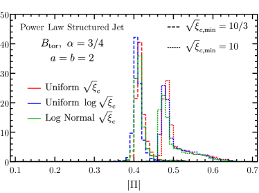
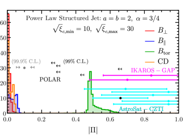
Figure 18: Left: Comparison of $|\Pi|$ obtained for different distributions of $\sqrt{\xi}_{c}$ when integrating over multiple pulses ($N_{p}=10$). The magnetic field configuration is that of a globally ordered toroidal field and the outflow has a power law angular structure. All three distributions sample $\sqrt{\xi}_{c}$ between $\sqrt{\xi}_{c,\min}\leq\sqrt{\xi}_{c}\leq\sqrt{\xi}_{c,\max}$ with $\sqrt{\xi}_{c,\max}=3\sqrt{\xi}_{c,\min}$. For the log-normal distribution $\mu=2.2$ and $\sigma=0.8$. Right: Comparison of $\Pi$ arising from synchrotron emission with different magnetic field configurations as well as from Compton drag (CD), for a power law structured jet, with measurements of GRB prompt emission polarization. Data with $\geq 3\sigma$ detection significance is shown with $1\sigma$ error bars. Upper limits with 99% confidence for the POLAR detected five GRBs are shown with black arrows, whereas $\Pi$ and limits derived from the joint analysis of these five GRBs are shown in gray (see Table 1). The Sharma et al. (2019) measurement of the average $\Pi=66^{+26}_{-27}\%$ ($\sim\!5.3\sigma$) over the emission episode obtained using AstroSat-CZTI is shown with a black dot with cyan error bars. For the models, the spectral index $\alpha=3/4$ where a different value might introduce a small variation, and $\sqrt{\xi}_{c}$ of the $N_{p}=10$ pulses is distributed uniformly.

8 Discussion & Conclusions

The measurement of linear polarization in the prompt emission of GRBs is of great interest as it offers very useful insights into the composition of the outflow and the structure of its magnetic field. This can further be used to pin down the exact radiation mechanism that gives rise to the prompt GRB gamma-ray emission. In this work, we discuss relevant radiation mechanisms that have been proposed to explain the prompt emission and that can also yield different levels of linear polarization. Furthermore, we have used the predictions for the polarization from these mechanisms (which depend on the jet geometry, viewing angle, magnetic field structure, and the spectral parameters), to ask the question what is the most likely explanation for a given polarization measurement. We have shown that either a single secure measurement of $50\%\lesssim\Pi\lesssim 65\%$ or measuring $\Pi\gtrsim 20\%$ in most GRBs within a large enough sample (using MC simulations), would strongly favor synchrotron emission from a transverse magnetic field ordered on angles $\gtrsim\!1/\Gamma$ around our line of sight (like a global toroidal field, $B_{\rm tor}$, for $1/\Gamma<\theta_{\rm obs}<\theta_{j}$).

In §3.5, we showed the predictions for $\Pi$ from synchrotron emission for three different magnetic field configurations in a top-hat jet. In the case of the random magnetic field that is completely in the plane of the ejecta ($B_{\perp}$), high levels of $\Pi$ are only achieved for a particular jet geometry and LOS. In this case, the jet has to be narrow with a uniform core and fairly sharp edges. On top of that, the observer’s LOS must be very close to the edge of the jet with $q\sim 1+\xi_{j}^{-1/2}$. The probability of observing close to the edge is $\sim(\Gamma\theta_{j})^{-1}$, where typically $\Gamma\theta_{j}\sim 10$, and so roughly $10\%$ of the bursts from a top-hat jet are seen slightly off-axis from near the edge of the jet. Majority of the bursts, especially at high redshift, must then be observed on-axis with $q<1$, otherwise the sharp drop in fluence for $q>1$ would render the burst too dim to be observed (let alone to be bright enough for their polarization to be measured). For this very reason, measurement of high levels of polarization arising for off-axis observers ($q>1$) when the outflow magnetic field is parallel to the local velocity vector everywhere ($B_{\parallel}$) will be challenging. In the case of a top-hat jet and for $q\lesssim 1$ only an ordered transverse magnetic field, such as a globally ordered toroidal field, in the outflow can yield the highest degree of polarization from synchrotron emission.

On the other hand, a structured jet offers a better chance for measuring higher $\Pi$ for off axis observers for all magnetic field configurations. However, as shown in §3.7, in the case of $B_{\perp}$ and $B_{\parallel}$ steep gradients in $\Gamma(\theta)$ are needed, otherwise it yields negligible polarization. In the case of the top-hat jet the necessity of having a sharp gradient in $\Gamma$ was replaced by the jet having a sharp edge. The $B_{\rm tor}$ configuration yet again yields the highest levels of polarization and does not require steep gradients in $\Gamma$. This model overcomes the problematic requirement of having a special LOS to observe a high degree of polarization, which makes this configuration robust from an observational standpoint. It also implies that majority of GRBs should show high polarization levels with $\Pi\gtrsim 20\%$. This can be potentially tested as the observed sample grows and measurements become better with upcoming more sensitive instruments.

An important consideration in the case of structured jets that are viewed off-axis is that compactness arguments require $\Gamma(\theta)$ to be shallow, e.g. $b\lesssim 1$ for a power law jet. However, such profiles don’t yield any detectable polarization when the magnetic field is not ordered on large scales, such as in the case of $B_{\perp}$ and $B_{\parallel}$; the same is also true for Compton drag. For steeper profiles, the observer can only see emission from close to the core and cannot be too off axis with $q\lesssim 2$. This constraint would also favour a large scale ordered magnetic field if $\Pi>20\%$ is observed even in a single burst.

The Compton drag model (§4) suffers from the same difficulty as the synchrotron model with $B_{\perp}$ and will mostly yield low levels of $\Pi$ unless $q\gtrsim 1$ and the jets are quite narrow. It was shown in Lazzati et al. (2004) that the top-hat jet must be narrow with $\xi_{j}\lesssim 25$ in order to obtain $\Pi\gtrsim 40\%$ while getting $\Pi\gtrsim 95\%$ for extremely narrow jets with $\xi_{j}=4\times 10^{-2}$. To distinguish between the synchrotron emission model, especially with $B_{\perp}$ and $B_{\parallel}$ field configurations, and the Compton drag scenario, one will have to rely on spectral modeling. In synchrotron emission the spectral index is rather limited to $-1/3\leq\alpha\lesssim 3/2$ which also limits the local maximum degree of polarization to $50\%\leq\Pi_{\max}\lesssim 75\%$. There is no such limitation on $\Pi_{\max}$ in the Compton drag model. Therefore, detecting spectrally harder bursts that violate the synchrotron line-of-death can be one way to discriminate between the two emission models.

In the photospheric emission model (§5), with no dissipation below the photosphere, $\Pi$ is rather limited to $\lesssim 15\%-20\%$. In order to achieve even this level of polarization the jet must be structured and have steep gradients in its energy per unit solid angle and $\Gamma$ with $\theta$. The angular structure of the jet is unclear and in the simplest scenario of a top-hat jet the photospheric model will yield negligible polarization for $q<1$. Spectrally, this model can be distinctly recognized as it produces a quasi-thermal spectrum, which has only been seen in a handful of bursts. On the other hand, dissipative photosphere models yield Band-like spectrum where the peak forms as a result of multiple Compton scatterings by heated electrons (or $e^{\pm}$-pairs) below the photosphere. Therefore, the peak itself will have negligible polarization, however, if the source of soft photons is synchrotron, which will be the dominant component below the peak, then the best case scenario can yield $\Pi\lesssim 50\%$ (Lundman, Vurm, & Beloborodov, 2018).

Finally, only an ordered magnetic field that has a coherence length comparable or larger than the size of the visible emitting region can consistently produce high levels of polarization with $\Pi\sim\Pi_{\max}$. However, if the size of coherent patches is smaller than that of the visible region so that $N_{p}$ patches contribute to a single emission episode, or alternatively $N_{p}$ intrinsicaly coherent (single-patch) but mutually incoherent pulses are integrated over in the same GRB, the this will reduce the maximum polarization by a factoir of $\sim\sqrt{N_{p}}$. In addition, since the PA will be randomly oriented for emission from any given patch (or pulse), time-resolved (pulse-resolved) polarization analysis should reveal significant oscillations of the PA between pulses. This prediction is in contrast with other field configurations where a constant PA should be observed, except for a $90^{\circ}$ flip. Inoue et al. (2011) studied the creation of ordered magnetic fields via the Richtmyer-Meshkov instability (RMI) in internal shocks using special relativistic magneto-hydrodynamic (MHD) simulations. It was realized there that the RMI would generate a large number ($\sim 10^{3}$) of incoherent patches which would lead to $\Pi\sim 2\%$. Measurements of higher levels of polarization would necessarily violate this estimate and point either to another mechanism of producing such ordered fields or the outflow having a large scale globally ordered field.

8.1 Implications of measuring $\Pi>20\%$

High degrees of polarization have been measured now in the prompt emission of several GRBs albeit with only modest statistical significance. A firm detection of $\Pi>20\%$ in several GRBs would point towards a globally ordered transverse magnetic field configuration in the outflow, for which a good candidate is toroidal magnetic field. It will also strongly indicate that the underlying dominant emission mechanism for the GRB prompt emission is synchrotron. For the toroidal field case and for the typical value of the jet parameter $\xi_{j}=10^{2}$, the range of the observed degree of polarization for a single burst is $0.4\lesssim\Pi/\Pi_{\max}\lesssim 0.85$ for different values of the spectral index $-1/3\leq\alpha\leq 3/2$, which corresponds to $20\%\lesssim\Pi\lesssim 68\%$, but it will never be larger than $75\%$. Also, in this case, both top-hat and structured jets would yield similar levels of polarization in a large sample of GRBs, with $\Pi\sim 40\%-50\%$ for $\alpha=3/4$. This will make it hard to distinguish between the two jet geometries based on polarization alone.

A firm detection of GRB gamma-ray polarization requires high-fluence sources, and in turn viewing angles within or very close to the jet core, $q\lesssim 1$. This limit on $q$ is further substantiated by compactness arguments. If only a small fraction ($\sim 10\%$) of GRBs show $\Pi\gtrsim 20\%$ this would favor models in which there is no net polarization for a spherical flow or LOS well within a uniform jet ($q<1-\xi_{j}^{-1/2}$), and require instead a special line of sight, $q\sim 1+\xi_{j}^{-1/2}$. Such models include emission from a top-hat jet and either synchrotron with $B_{\perp}$ or $B_{\parallel}$, or Compton drag. It would naturally also disfavor synchrotron emission from a large scale ordered magnetic field such as $B_{\rm tor}$.

Statistically significant measurements of GRB prompt emission polarization will increase with the advent of new high-energy polarimeters and with the observations of very bright GRBs with currently operating instruments (see, e.g. McConnell, 2017, for a review of various instruments). Comparison of the moderately statistically significant measurements ($\gtrsim 3\sigma$) with the different emission models and magnetic field configurations strongly favour the existence of a toroidal (or other transverse and globally ordered) magnetic field in the outflow and that the underlying prompt GRB emission mechanism is synchrotron.

The models considered in this work have assumed an axisymmetric jet or outflow angular structure, which leads to a constant PA, $\theta_{p}$, or at most a change of $\Delta\theta_{p}=90^{\circ}$ in $\theta_{p}$. However, it is important to keep in mind that non-axisymmetric effects can lead to arbitrary changes in $\theta_{p}$. In particular, a “mini-jet” type of emission model, in which each spike is produced by plasma moving relativistically w.r.t the bulk outflow frame and in a random direction within that frame, could produce a random $\theta_{p}$ for each pulse. In such a case the polarization from different pulses would add up incoherently. This is analogous to the patchy shell model in which the outflow has a single bulk $\Gamma$ but the angular distribution of the emission brightness is highly non-uniform. However, such strong variations within the visible region of $1/\Gamma$ around the LOS, which is also in lateral causal contact, would be very hard to maintain in the flow, while a mini-jet model does not suffer from such a difficulty.

Appendix A Time-integrated polarization for an ultra-relativistic structured jet

Here we present a general formalism for obtaining time-integrated polarization for a structured jet that is emitting synchrotron radiation. This can be easily generalized further to other radiation mechanisms discussed in this work. Also, general expressions valid for a uniform jet are pointed out. The flow is assumed to be ultra-relativistic with $\Gamma\gg 1$ and the emission is assumed to arise from an infinitely thin shell. The instantaneous degree of polarization follows from Eq. (5,8,9) and can be expressed as

$$\Pi(t_{z})=\frac{Q(t_{z})}{I(t_{z})}=\frac{\int\delta_{D}^{3}L^{\prime}_{\nu^{\prime}}\Pi^{\prime}\cos(2\theta_{p})d\tilde{\Omega}}{\int\delta_{D}^{3}L^{\prime}_{\nu^{\prime}}d\tilde{\Omega}}$$ (101)

where $t_{z}$ is the arrival time of photons in the cosmological rest frame of the source and is expressed through the equal arrival time condition (Eq. 26 in the text)

$$\frac{t_{\rm obs}}{(1+z)}\equiv t_{z}=t-\frac{r\tilde{\mu}}{c}~{}.$$ (102)

The time-integrated polarization is obtained from

$$\Pi=\frac{\int_{t_{z,0}}^{t_{z,\max}}Q(t_{z})dt_{z}}{\int_{t_{z,0}}^{t_{z,\max}}I(t_{z})dt_{z}}$$ (103)

where $t_{z,0}$ is the arrival time of the first photon. To analytically integrate over all the arrival times, we can express $dt_{z}$ in terms of $dr$ from the equal arrival time condition for constant $\tilde{\mu}$ and $\tilde{\varphi}$, such that

$$dt_{z}=\frac{(1-\beta\tilde{\mu})}{\beta c}dr=\frac{\delta_{D}^{-1}}{\Gamma\beta c}dr\approx\frac{\delta_{D}^{-1}}{\Gamma c}dr$$ (104)

For a uniform jet, the factor of $\Gamma$ would be constant with polar angle $\theta$ (and also assumed constant with $r$ here) and cancel in the final expression for $\Pi$, however, it won’t cancel if the jet is structured since $\Gamma=\Gamma(\theta)$.

Next, the radial integral can be collapsed to a delta function in $r$ since the integrand or any other parameters are assumed to be independent of $r$, which simplifies the treatment and yields the time-integrated polarization

$$\Pi=\frac{Q}{I}=\frac{\displaystyle\int\frac{\delta_{D}^{2}}{\Gamma}L^{\prime}_{\nu^{\prime}}\Pi^{\prime}\cos(2\theta_{p})d\tilde{\Omega}}{\displaystyle\int\frac{\delta_{D}^{2}}{\Gamma}L^{\prime}_{\nu^{\prime}}d\tilde{\Omega}}~{}.$$ (105)

We can express $d\tilde{\Omega}=d\tilde{\mu}d\tilde{\varphi}$, where for small angles $d\tilde{\mu}\approx\tilde{\theta}d\tilde{\theta}=\frac{1}{2}d(\tilde{\theta}^{2})=\frac{1}{2\Gamma_{c}^{2}}d(\Gamma_{c}^{2}\tilde{\theta}^{2})=\frac{1}{2\Gamma_{c}^{2}}d\tilde{\xi}$. Here we have normalized the polar angle measured from the LOS in terms of the beaming angle of the core emission $\Gamma_{c}^{-1}$ in a structured jet, which is a constant, and further defined the useful quantity $\tilde{\xi}\equiv\Gamma_{c}^{2}\tilde{\theta}^{2}$. Notice that this is the same parameterization as used in Eq. (17) since for a top-hat jet $\Gamma\to\Gamma_{c}$ as it doesn’t vary with polar angle $\theta$. The Doppler factor can also be expressed using the same parameterization in the ultra-relativistic limit, which yields

$$\delta_{D}=\frac{1}{\Gamma(1-\beta\tilde{\mu})}\approx\frac{2\Gamma}{1+\Gamma^{2}\tilde{\theta}^{2}}=2\Gamma_{c}\frac{\hat{\Gamma}}{1+\hat{\Gamma}^{2}\tilde{\xi}}=2\Gamma_{c}\frac{\hat{\Gamma}}{1+\hat{\xi}}~{},$$ (106)

where $\hat{\xi}\equiv\Gamma^{2}\tilde{\theta}^{2}=\hat{\Gamma}^{2}\tilde{\xi}$. Again, for a uniform jet $\hat{\Gamma}\equiv\Gamma/\Gamma_{c}=1$ and therefore $\delta_{D}\propto(1+\tilde{\xi})^{-1}$.

If the azimuthally symmetric jet has angular structure, its kinetic energy per unit solid angle, $\epsilon(\theta)\equiv dE_{k}(\theta)/d\Omega$, and LF, $\Gamma(\theta)$, would vary with polar angle away from the jet symmetry axis. The corresponding isotropic equivalent kinetic energy is given by $E_{k,\rm iso}(\theta)=4\pi\epsilon(\theta)$. If this energy is radiated with efficiency $\epsilon_{\gamma}$ over a lab-frame time $\Delta t_{\rm lab}=\Delta r/\beta c$, then the radiated power, which is a Lorentz invariant, can be expressed as

$$L^{\prime}_{\rm iso}(\theta)=\frac{dE_{\rm rad,iso}^{\prime}}{dt^{\prime}}=\frac{dE_{\rm rad,iso}}{dt_{\rm lab}}=\frac{4\pi\epsilon_{\gamma}\epsilon(\theta)}{(\Delta r/\beta c)}~{}.$$ (107)

Next we assume that the normalization of the fluid-frame isotropic spectral luminosity, without the factor $\Lambda$ (defined in Eq. (18) in the text) that is associated to a particular LOS, is given by an infinite power law, such that $L^{\prime}_{\nu^{\prime}}=L^{\prime}_{\nu_{p}^{\prime}}(\nu^{\prime}/\nu_{p}^{\prime})^{-\alpha}$ for $\nu^{\prime}\geq\nu_{p}^{\prime}$, where $\nu_{p}^{\prime}$ is a characteristic frequency at which most of the power is radiated, i.e. where $\nu^{\prime}L^{\prime}_{\nu^{\prime}}$ peaks. Integration over $\nu^{\prime}$, while neglecting any contribution from frequencies $\nu^{\prime}<\nu_{p}^{\prime}$ (accounting for this contribution would slightly modify the factor $\chi$ below, which would generally remain of order unity), which is assumed negligible here, then yields the bolometric power,

$$L^{\prime}_{\rm iso}=\int_{\nu_{p}^{\prime}}^{\nu_{\max}^{\prime}}d\nu^{\prime}L^{\prime}_{\nu^{\prime}}=\frac{\nu_{p}^{\prime}L^{\prime}_{\nu_{p}^{\prime}}}{(\alpha-1)}\left[1-\left(\frac{\nu_{\max}^{\prime}}{\nu_{p}^{\prime}}\right)^{1-\alpha}\right]=\chi\nu_{p}^{\prime}L^{\prime}_{\nu_{p}^{\prime}}~{}$$ (108)

for $\alpha>1$. When $(\nu^{\prime}_{\max}/\nu_{p}^{\prime})\gg 1$, $\chi\to(\alpha-1)^{-1}$.

Equating Eqs. (107 & 108) yields the comoving spectral luminosity in terms of the energy per unit solid angle of the flow, $\epsilon=\epsilon_{c}\Theta^{-a}$, which e.g. is assumed here to vary as a power law,

$$L^{\prime}_{\nu^{\prime}}=\frac{4\pi\epsilon_{\gamma}\epsilon(\theta)}{\chi\nu_{p}^{\prime}(\Delta r/\beta c)}\left(\frac{\nu^{\prime}}{\nu^{\prime}_{p}}\right)^{-\alpha}=\frac{4\pi\epsilon_{\gamma}\beta c}{\chi\nu_{p}^{\prime}\Delta r}\left(\frac{\nu^{\prime}}{\nu^{\prime}_{p}}\right)^{-\alpha}\epsilon_{c}\Theta^{-a}\ ,$$ (109)

When assuming a similar power law dependence for $\Gamma(\theta)-1$ (the kinetic energy per unit rest energy), the following expressions (as described by Eq. (50) in the text) are obtained,

$$\displaystyle\frac{L^{\prime}_{\nu^{\prime}}}{L^{\prime}_{\nu^{\prime},0}}=\Theta^{-a},\quad\quad\frac{\Gamma(\theta)-1}{\Gamma_{c}-1}=\Theta^{-b}$$ (110)

$$\Theta=\sqrt{1+\frac{\theta^{2}}{\theta_{c}^{2}}}=\sqrt{1+\frac{\Gamma_{c}^{2}\theta^{2}}{\Gamma_{c}^{2}\theta_{c}^{2}}}=\sqrt{1+\frac{\xi}{\xi_{c}}}~{}.$$ (111)

In the ultra-relativistic limit, $(\Gamma(\theta)-1)/(\Gamma_{c}-1)\approx\Gamma(\theta)/\Gamma_{c}\equiv\hat{\Gamma}(\theta)$. Plugging in Eqs. (109 & 110) and the factor $\Lambda$ in Eq. (105) gives

$$\Pi=\frac{Q}{I}=\frac{\displaystyle\int\delta_{D}^{2+\alpha}\hat{\Gamma}^{-1}\Theta^{-a}\Lambda\Pi^{\prime}\cos(2\theta_{p})d\tilde{\Omega}}{\displaystyle\int\delta_{D}^{2+\alpha}\hat{\Gamma}^{-1}\Theta^{-a}\Lambda d\tilde{\Omega}}~{}.$$ (112)

Here we have explicitly assumed $\nu_{p}^{\prime}$ to be a constant, however, in general $\nu_{p}^{\prime}=\nu_{p}^{\prime}(t^{\prime},\theta)$. In addition, the above expression is valid so long $\nu^{\prime}=\delta_{D}^{-1}\nu>\nu_{p}^{\prime}$ or in general, $\nu^{\prime}$ falls in the same power law segment for which $L^{\prime}_{\nu^{\prime}}\propto\nu^{\prime-\alpha}$.

The emissivity and $\Gamma(\theta)$ profiles, and the variable $\hat{\xi}$, depend on $\xi\propto\theta^{2}$ and the relation between these is obtained from the geometry of the problem. In general,

$$\mu=\mu_{\rm obs}\tilde{\mu}-\cos\tilde{\varphi}\sqrt{(1-\mu_{\rm obs}^{2})(1-\tilde{\mu}^{2})}~{},$$ (113)

where $\mu\equiv\cos\theta$, $\mu_{\rm obs}\equiv\cos\theta_{\rm obs}=\cos(q\theta_{c})$ with $q=\theta_{\rm obs}/\theta_{c}$, and $\tilde{\mu}\equiv\cos\tilde{\theta}$. For the ultra-relativistic case, and in the small angle limit, the above relation simplifies to

$$\theta^{2}\approx\tilde{\theta}^{2}+q^{2}\theta_{c}^{2}+2q\tilde{\theta}\theta_{c}\cos\tilde{\varphi}$$ (114)

$$\Rightarrow \xi=\tilde{\xi}+q^{2}\xi_{c}+2q\sqrt{\tilde{\xi}\xi_{c}}\cos\tilde{\varphi}~{},$$ (115)

where the second equation was obtained by simply multiplying both sides by $\Gamma_{c}$. This defines all the relevant set of equations that are needed to calculate time-integrated $\Pi$, for which the final expression becomes

$$\Pi=\frac{\int_{0}^{\tilde{\xi}_{\max}}d\tilde{\xi}\int_{0}^{2\pi}d\tilde{\varphi}\delta_{D}^{2+\alpha}\hat{\Gamma}^{-1}\Lambda(\hat{\xi},\tilde{\varphi})\Theta^{-a}\Pi^{\prime}(\hat{\xi},\tilde{\varphi})\cos(2\tilde{\varphi})}{\int_{0}^{\tilde{\xi}_{\max}}d\tilde{\xi}\int_{0}^{2\pi}d\tilde{\varphi}\delta_{D}^{2+\alpha}\hat{\Gamma}^{-1}\Lambda(\hat{\xi},\tilde{\varphi})\Theta^{-a}}~{},$$ (116)

where $\tilde{\xi}_{\max}>10^{2}$ is chosen appropriately which guarantees a converged result.

References

- Abramowicz, Novikov, & Paczyński (1991) Abramowicz, M. A., Novikov, I. D., & Paczyński, B. 1991, ApJ, 369, 175
- Band et al. (1993) Band, D. et al. 1993, ApJ, 413, 281
- Begelman & Sikora (1987) Begelman, M. C. & Sikora, M. 1987, ApJ, 322, 650
- Bégué et al. (2013) Bégué, D., Siutsou, I. A., & Vereshchagin, G. V. 2013, ApJ, 767, 139
- Beloborodov (2010) Beloborodov, A. M. 2010, MNRAS, 407, 1033
- Beloborodov (2011) Beloborodov, A. M. 2011, ApJ, 737, 68
- Beloborodov & Mészáros (2017) Beloborodov, A. M. & Mészáros, P. 2017, Space Sci. Rev., 207, 87
- Beniamini & Nakar (2018) Beniamini, P. & Nakar, E. 2018, ArXiv eprints, arXiv:1808.07493
- Burgess et al. (2018) Burgess, J. M. et al. 2018, arXiv eprints: arXiv:1810.06965
- Burgess et al. (2019) Burgess, J. M. et al. 2019, arXiv eprints: arXiv:1901.04719
- Chattopadhyay et al. (2017) Chattopadhyay, T. et al. 2017, ArXiv eprints, arXiv:1707.06595
- Coburn & Boggs (2003) Coburn, W. & Boggs, S. E. 2003, Nature, 423, 415
- Covino et al. (2003) Covino, S., Ghisellini, G., Lazzati, D., & Malesani, D. 2003, in ASP Conf. Ser. 312, Third Rome Workshop on Gamma-Ray Bursts in the Afterglow Era, ed. M. Feroci, F. Frontera, N. Masetti, & L. Piro (San Francisco: ASP), 169
- Covino & Götz (2016) Covino, S. & Götz, D. 2016, A&AT, 29, 205
- Crider et al. (1997) Crider, A., Liang E. P., & Smith, I. A. 1997, ApJ, 479, L39
- Chand et al. (2018a) Chand, V. et al. 2018a, ApJ, 862, 154
- Chand et al. (2018b) Chand, V. et al. 2018b, eprint (arXiv:1807.01737)
- Chandrasekhar (1960) Chandrasekhar, S. 1960, Radiative Transfer (New York: Dover)
- Chang & Lin (2014) Chang, Z. & Lin, H.-N. 2014, ApJ, 765, 36
- Corsi et al. (2018) Corsi, A., et al. 2018, ApJ, 861, L10
- Daigne & Mochkovitch (1998) Daigne, F. & Mochkovitch, R. 1998, MNRAS, 296, 275
- Deng et al. (2016) Deng, W. et al. 2016, ApJ, 821, L12
- Drenkhahn (2002) Drenkhahn, G. 2002, A&A, 387, 714
- Drenkhahn & Spruit (2002) Drenkhahn, G. & Spruit, H. C. 2002, A&A, 391, 1141
- Eichler & Levinson (2000) Eichler, D. & Levinson, A. 2003, ApJ, 529, 146
- Eichler & Levinson (2003) Eichler, D. & Levinson, A. 2003, ApJ, 596, L147
- Eichler & Levinson (2004) Eichler, D. & Levinson, A. 2004, ApJ, 614, L13
- Giannios (2006) Giannios, D. 2006, A&A, 457, 763
- Giannios (2008) Giannios, D. 2008, A&A, 480, 305
- Gill & Granot (2019) Gill, R. & Granot, J. 2019, arXiv e-prints: arXiv:1910.05687
- Gill & Granot (2018) Gill, R. & Granot, J. 2018, MNRAS, 475, L1
- Gill & Thompson (2014) Gill, R. & Thompson, C. 2014, ApJ, 796, 81
- Ghisellini & Celotti (1999) Ghisellini, G. & Celotti, A. 1999, ApJ, 511, L93
- Ghisellini & Lazzati (1999) Ghisellini, G. & Lazzati, D. 1999, MNRAS, 309, L7
- Ghirlanda, Celotti, Ghisellini (2003) Ghirlanda, G., Celotti, A., & Ghisellini, G. 2003, A&A, 406, 897
- Ghirlanda et al. (2013) Ghirlanda, G. et al. 2013, MNRAS, 428, 1410
- Ghirlanda et al. (2015) Ghirlanda, G. et al. 2015, MNRAS, 420, 483
- Goodman (1986) Goodman, J. 1986m ApJ, 308, L47
- Götz et al. (2009) Götz, D. et al. 2009, ApJ, 695, L208
- Götz et al. (2013) Götz, D. et al. 2013, MNRAS, 431, 3550
- Götz et al. (2014) Götz, D. et al. 2014, MNRAS, 444, 2776
- Granot (2003) Granot, J. 2003, ApJ, 596, L17
- Granot (2005) Granot, J. 2005, ApJ, 631, 1022
- Granot, Komissarov & Spitkovsky (2011) Granot, J., Komissarov, S. S., & Spitkovsky, A. 2011, MNRAS, 411, 1323
- Granot & Sari (2002) Granot, J. & Sari, R. 2002, ApJ, 568, 820
- Granot, Cohen-Tanugi, & Do Couto E Silva (2008) Granot, J., Cohen-Tanugi, J., & Do Couto E Silva, E. 2008, ApJ, 677, 92
- Granot et al. (2015) Granot, J. et al. 2015, Space Sci. Rev., 191, 471
- Granot & Kumar (2003) Granot, J. & Kumar, P. 2003, ApJ, 591, 1086
- Granot & Königl (2003) Granot, J. & Königl, A. 2003, ApJ, 594, L83
- Granot et al. (2002) Granot, J. et al. 2002, ApJ, 570, L61
- Granot, Piran, & Sari (1999a) Granot, J., Piran, T., & Sari, R. 1999a, ApJ, 513, 679
- Granot, Piran, & Sari (1999b) Granot, J., Piran, T., & Sari, R. 1999b, ApJ, 527, 236
- Granot & Ramirez-Ruiz (2011) Granot, J. & Ramirez-Ruiz, E. 2011, in Kouveliotou, C., Woosley, S. E. Wijers, R. A. M. J., Gamma-ray Bursts, Cambridge Univ. Press, Cambridge (arXiv:1012.5101)
- Granot & Taylor (2005) Granot, J. & Taylor, G. 2005, ApJ, 625, 263
- Gruzinov (1999) Gruzinov, A. 1999, ApJ, 525, L29
- Gruzinov & Waxman (1999) Gruzinov, A. & Waxman, E. 1999, ApJ, 511, 852
- Hascoët et al. (2012) Hascoët, R., Daigne, F., Mochkovitch, R., & Vennin, V. 2012, MNRAS, 421, 525
- Inoue et al. (2011) Inoue, T. et al. 2011, ApJ, 734, 77
- Ito et al. (2014) Ito, H. et al. 2014, ApJ, 789, 159
- Kalemci et al. (2007) Kalemci, E. et al. 2007, ApJS, 169, 75
- Korchakov & Syrovatskii (1961) Korchakov, A. A. & Syrovatskii, S. I. 1961, Soviet Astr.–A. J., 5, 678
- Kumar & Granot (2003) Kumar, P. & Granot, J. 2003, ApJ, 591, 1075
- Kumar & Narayan (2009) Kumar, P. & Narayan, R. 2009, MNRAS, 395, 472
- Kumar & Zhang (2015) Kumar, P. & Zhang, B. 2015, Phys. Rep., 561, 1
- Laskar et al. (2019) Laskar, T. et al. 2019, ApJ, 878, L26
- Lazar et al. (2009) Lazar, A., Nakar, E., & Piran, T. 2009, ApJ, 695, L10
- Lazzati (2006) Lazzati, D. 2006, New J. Phys., 8, 131
- Lazzati et al. (2000) Lazzati, D., Ghisellini, G., Celotti, A., & Rees, M. J. 2000, 529, L17
- Lazzati et al. (2004) Lazzati, D. et al. 2004, MNRAS, 347, L1
- Lazzati, Morsony, & Begelman (2009) Lazzati, D., Morsony, Morsony, B. J., & Begelman, M. C. 2009, ApJ, 700, L47
- Lazzati & Begelman (2006) Lazzatti, D. & Begelman, M. C. 2006, ApJ, 725, 1137
- Lowell et al. (2017) Lowell, A. W. et al. 2017, ApJ, 848, 119
- Lundman, Pe’er, & Ryde (2014) Lundman, C., Pe’er, A. & Ryde, F. 2014, MNRAS, 440, 3292
- Lundman, Vurm, & Beloborodov (2018) Lundman, C., Vurm, I., & Beloborodov, A. M. 2018, ApJ, 856, 145
- Lyubarsky & Kirk (2001) Lyubarsky, Y. & Kirk, J. G. 2001, ApJ, 547, 437
- Lyutikov & Blandford (2003) Lyutikov, M. & Blandford, R. 2003, ArXiv eprints, arXiv:astro-ph/0312347
- Lyutikov, Pariev, & Blandford (2003) Lyutikov, M., Pariev, V. I., & Blandford, R. 2003, ApJ, 597, 998
- Matsumoto, Nakar, & Piran (2019) Matsumoto, T., Nakar, E., & Piran, T. 2019, MNRAS, 486, 1563
- Mao & Wang (2013) Mao, J. & Wang, J. 2013, ApJ, 776, 17
- Mao & Wang (2017) Mao, J. & Wang, J. 2017, ApJ, 838, 78
- McConnell (2017) McConnell, M. L. 2017, NewAR, 76, 1
- McGlynn et al. (2007) McGlynn, S. et al. 2007, A&A, 466, 895
- Medvedev (2000) Medvedev, M. V. 2000, ApJ, 540, 704
- Medvedev & Loeb (1999) Medvedev, M. V. & Loeb, A. 1999, ApJ, 526, 697
- Mészáros & Rees (2000) Mészáros, P. & Rees, M. J. 2000, ApJ, 530, 292
- Mooley et al. (2018) Mooley, K. P.., et al. 2018, Nature, 561, 355
- Mundell et al. (2013) Mundell, C. G. et al. 2013, Nature, 504, 119
- Nakar & Oren (2004) Nakar, E., & Oren, Y. 2004, ApJ, 602, L97
- Nakar, Piran, & Waxman (2003) Nakar, E., Piran, T., & Waxman, E. 2003, JCAP, 10, 005
- Narayan & Kumar (2009) Narayan, R. & Kumar, P. 2009, MNRAS, 394, L117
- Nava, Nakar, & Piran (2016) Nava, L., Nakar, E., & Piran, T. 2016, MNRAS, 455, 1594
- Oganesyan et al. (2017) Oganesyan, G. et al. 2017, ApJ, 846, 137
- Paczyński (1986) Paczyński, B. 1986, ApJ, 308, L43
- Papathanassiou & Mészáros (1996) Papathanassiou, H. & Mészáros, P. 1996, ApJ, 471, L91
- Pearce et al. (2019) Pearce, M. et al. 2019, APh, 104, 54
- Pe’er & Ryde (2011) Pe’er, A. & Ryde, F. 2011, ApJ, 732, 49
- Piran, Sari, & Zou (2009) Piran, T., Sari, R., & Zou, Y. C. 2009, MNRAS, 1107, 1113
- Preece et al. (1998) Preece, R. D., Briggs, M. S., Mallozzi, R. S. et al. 1998, ApJ, 506, L23
- Preece et al. (2002) Preece, R. D., Briggs, M. S., Mallozzi, R. S. et al. 2002, ApJ, 518, 1248
- Prosekin et al. (2016) Prosekin, A. Y., Kelner, S. R., & Aharonian, F. A. et al. 2016, Phys. Rev. D, 94, 063010
- Ravasio et al. (2018) Ravasio, M. E. et al. 2018, A&A, 613, A16
- Rees & Mészáros (1994) Rees, M. J. & Mészáros, P. 1994, ApJ, 430, L93
- Rees & Mészáros (2005) Rees, M. J. & Mészáros, P. 2005, ApJ, 628, 847
- Rossi, Lazzati, & Rees (2002) Rossi, E. M., Lazzati, D., & Rees, M. J. 2002, MNRAS, 332, 945
- Rossi et al. (2004) Rossi, E. M., Lazzati, D., Salmonson, J. D. et al. 2004, MNRAS, 354, 86
- Rybicki & Lightman (1979) Rybicki, G. B., & Lightman, A. P. 1979, Radiative Processes in Astrophysics, Wiley & Sons (New York)
- Rutledge & Fox (2004) Rutledge, R. E. & Fox, D. B. 2004, MNRAS, 350, 1288
- Sari (1999) Sari, R. 1999, ApJ, 524, L43
- Sari & Piran (1997) Sari, R. & Piran, T. 1997, MNRAS, 287, 110
- Salafia et al. (2015) Salafia, O. S. et al. 2015, MNRAS, 450, 3549
- Singh et al. (2014) Singh, K. P. et al. 2014, SPIE, 9144, 1
- Sironi & Spitkovsky (2011) Sironi, L., & Spitkovsky, A. 2011, ApJ, 726, 75
- Sharma et al. (2019) Sharma, V., Iyyani, S., Bhattacharya, D. et al. 2019, ApJL, 882, L10
- Shaviv & Dar (1995) Shaviv, N. J. & Dar, A. 1995, ApJ, 447, 863
- Sobolev (1963) Sobolev, V. V. 1963, A Treatise on Radiative Transfer (Princeton, NJ: Van Nostrand-Reinhold)
- Spruit et al. (2001) Spruit, H. C., Daigne, F., & Drenkhahn, G. 2001, A&A, 369, 694
- Steele et al. (2009) Steele, I. A. et al. 2009, Nature, 462, 767
- Thompson (1994) Thompson, C. 1994, MNRAS, 270, 480
- Thompson & Gill (2014) Thompson, C. & Gill, R. 2014, ApJ, 791, 30
- Toma et al. (2009) Toma, K. et al. 2009, ApJ, 698, 1042
- Toma (2013) Toma, K. 2013, ArXiv eprints, arXiv:1308.5733
- Vurm & Beloborodov (2016) Vurm, I. & Beloborodov, A. M. 2016, ApJ, 831, 175
- Vurm, Lyubarsky, & Piran (2013) Vurm, I., Lyubarsky, Y., & Piran, T. 2013, ApJ, 764, 143
- Waxman (2003) Waxman, E. 2003, Nature, 423, 388
- Wigger et al. (2004) Wigger, C. et al. 2004, ApJ, 613, 1088
- Yamazaki et al. (2003) Yamazaki, R., Ioka, K., & Nakamura, T. 2003, ApJ, 606, L33
- Yonetoku et al. (2011a) Yonetoku, D. et al. 2011, PASJ, 63, 625
- Yonetoku et al. (2011b) Yonetoku, D. et al. 2011, ApJ, 743, L30
- Yonetoku et al. (2012) Yonetoku, D. et al. 2012, ApJ, 785, L1
- Zhang et al. (2019) Zhang, S.-N. et al. 2019, Nature Astronomy, doi:10.1038/s41550-018-0664-0
- Zhang & Mészáros (2002) Zhang, B. & Mészáros, P. 2002, ApJ, 571, 876
- Zhang & Yan (2011) Zhang, B. & Yan, H. 2011, ApJ, 726, 90