Link Prediction in Networks with Core-Fringe Data

Abstract.

Data collection often involves the partial measurement of a larger system. A common example arises in collecting network data: we often obtain network datasets by recording all of the interactions among a small set of core nodes, so that we end up with a measurement of the network consisting of these core nodes along with a potentially much larger set of fringe nodes that have links to the core. Given the ubiquity of this process for assembling network data, it is crucial to understand the role of such a “core-fringe” structure.

Here we study how the inclusion of fringe nodes affects the standard task of network link prediction. One might initially think the inclusion of any additional data is useful, and hence that it should be beneficial to include all fringe nodes that are available. However, we find that this is not true; in fact, there is substantial variability in the value of the fringe nodes for prediction. Once an algorithm is selected, in some datasets, including any additional data from the fringe can actually hurt prediction performance; in other datasets, including some amount of fringe information is useful before prediction performance saturates or even declines; and in further cases, including the entire fringe leads to the best performance. While such variety might seem surprising, we show that these behaviors are exhibited by simple random graph models.

1. Introduction

In a wide range of data analysis problems, the underlying data typically comes from partial measurement of a larger system. This is a ubiquitous issue in the study of networks, where the network we are analyzing is almost always embedded in some larger surrounding network (Kim and Leskovec, 2011; Kossinets, 2006; Laumann et al., 1989). Such considerations apply to systems at all scales. For example, when studying the communication network of an organization, we can potentially gain additional information if we know the structure of employee interactions with people outside the organization as well (Romero et al., 2016). A similar issue applies to large-scale systems. If we are analyzing the links within a large online social network, or the call traffic data from a large telecommunications provider, we could benefit from knowing the interactions that members of these systems have with individuals who are not part of the platform, or who do not receive service from the provider.

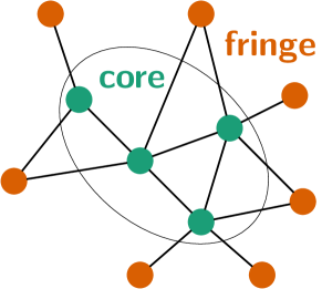
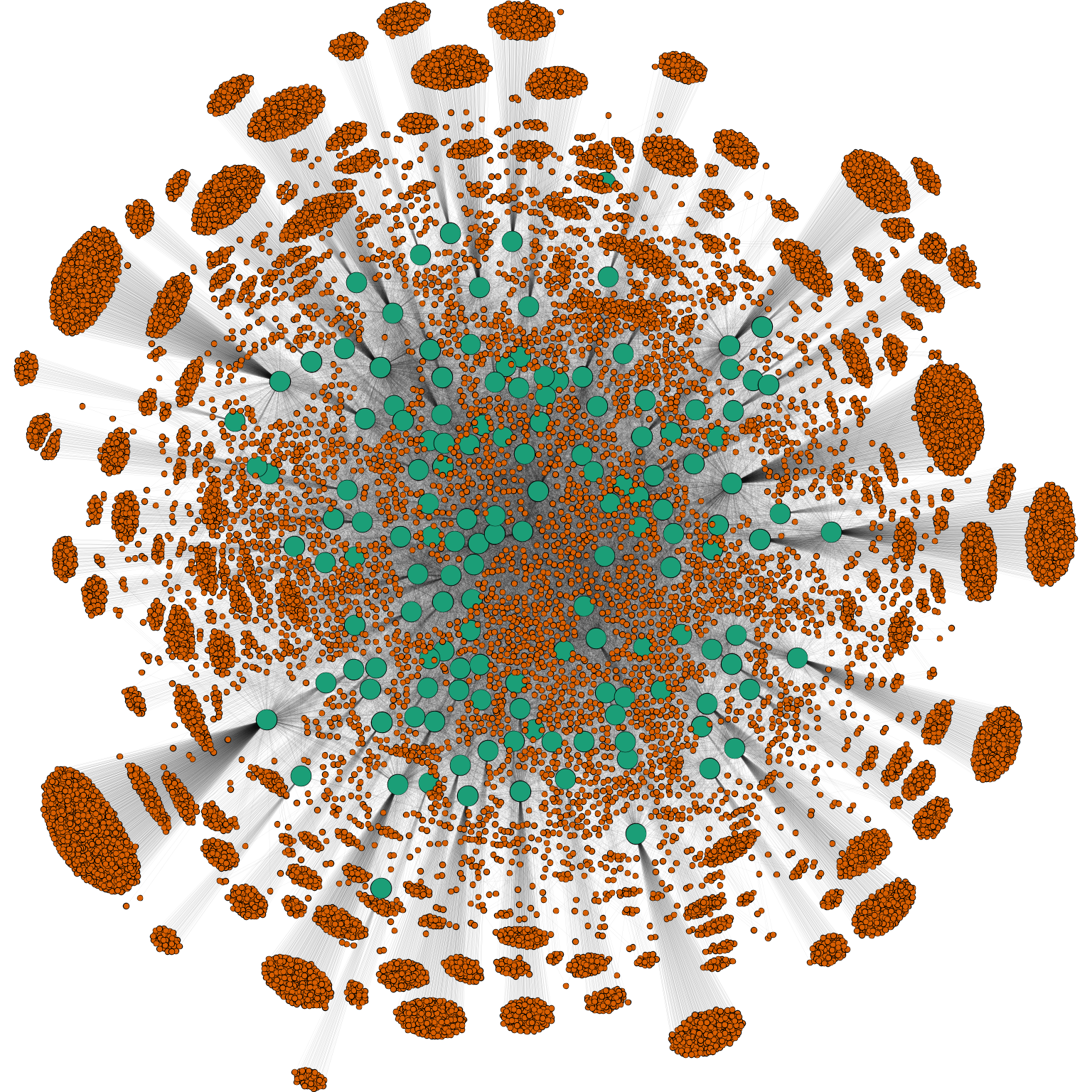
Figure 1. Core-fringe structure. (Left) Illustrative network with labeled core-fringe structure (core nodes in green and fringe nodes in orange). We observe all of the links involving core nodes (in green). Each edge is between two core nodes or between one core and one fringe node. (Right) Core-fringe structure in the Enron email network, which results from data collection—the core nodes in green correspond to the roughly 150 accounts whose emails were released as part of a federal investigation (Klimt and Yang, 2004). Here, the number of fringe nodes is orders of magnitude larger than the number of core nodes.

Network data can therefore be viewed as having a core-fringe structure (following the terminology of our previous work (Benson and Kleinberg, 2018)): we collect data by measuring all of the interactions involving a core set of nodes, and in the process we also learn about the core’s interaction with a typically larger set of additional nodes—the fringe—that does not directly belong to the measured system. Figure 1 illustrates the basic structure schematically and also in a typical real-life scenario: If we collect a dataset by measuring all email communication to and from the executives of a company (the core), then the data will also include links to people outside this set with whom members of the core exchanged email (the fringe). We thus have two kinds of links: links between two members of the core, and links between a member of the core and a member of the fringe. Links between fringe members are not visible, even though we are aware of both fringe nodes through their interactions with the core.

Despite the fundamental role of core-fringe structure in network data and a long history of awareness of this issue in the social sciences (Laumann et al., 1989), there has been little systematic attention paid to its implications in basic network inference tasks. If we are trying to predict network structure on a measured set of core nodes, what is the best way to make use of the fringe? Is it even clear that incorporating the fringe nodes will help? To study these questions, it is important to have a concrete task on the network where notions of performance as a function of available data are precise.

The present work: Core-fringe link prediction.  In this paper, we study the role of core-fringe structure through one of the standard network inference problems: link prediction (Liben-Nowell and Kleinberg, 2007; Lü and Zhou, 2011). Link prediction is a problem in which the goal is to predict the presence of unseen links in a network. Links may be unseen for a variety of reasons, depending on the application—we may have observed the network up to a certain point in time and want to forecast new links, or we may have collected a subset of the links and want to know which additional ones are present.

Abstractly, we will think of the link prediction problem as operating on a graph $G=(V,E)$ whose edges are divided into a set of observed edges and a set of unseen edges. From the network structure on the observed edges, we would like to predict the presence of the unseen edges as accurately as possible. A large range of heuristics have been proposed for this problem, many of them based on the empirical principle that nodes with neighbors in common are generally more likely to be connected by a link (Liben-Nowell and Kleinberg, 2007; Lü and Zhou, 2011; Rapoport, 1953).

The issue of core-fringe structure shows up starkly in the link prediction problem. Suppose the graph $G$ has nodes that are divided into a core set $C$ and a fringe set $F$, and our goal is to predict unseen links between pairs of nodes in the core. One option would be to perform this task using only the portion of $G$ induced on the core nodes. But we could also perform the task using larger amounts of $G$ by taking the union of the core nodes with any subset of the fringe, or with all of the fringe. The key question is how much of the fringe we should include if our goal is to maximize performance on the core; existing work provides little guidance about this question.

How much do fringe nodes help in link prediction?  We explore this question in a broad collection of network datasets derived from email, telecommunication, and online social networks. For concreteness, our most basic formulation draws on common-neighbor heuristics to answer the following version of the link prediction question: given two pairs of nodes drawn from the core, $\{u,v\}$ and $\{w,z\}$, which pair is more likely to be connected by a link? (In our evaluation framework, we will focus on cases in which exactly one of these pairs is truly connected by a link, thus yielding a setting with a clear correct answer.) To answer this question, we could use information about the common neighbors that $\{u,v\}$ and $\{w,z\}$ have only in the core, or also in any subset of the fringe. How much fringe information should we use, if we want to maximize our probability of getting the correct answer?

It would be natural to suspect that using all available data, i.e., including all of the fringe nodes, would maximize performance. What we find, however, is a wide range of behaviors. In some of our domains—particularly the social-networking data—link prediction performance increases monotonically in the amount of fringe data used, though with diminishing returns as we incorporate the entire fringe. In the other domains, however, we find a number of instances where using an intermediate level of fringe, i.e., a proper subset of the fringe nodes, yields a performance that dominates the option of including all of the fringe or none of it. And there are also cases where prediction is best when we ignore the fringe entirely. Given that proper subsets of the fringe can yield better performance than either extreme, we also consider the process of selecting a subset of the fringe; in particular, we study different natural orderings of the fringe nodes and then select a subset by searching over prefixes of these orderings.

To try understanding this diversity of results, we turn to basic random graph models, adapting them to capture the problem of link prediction in the presence of core-fringe structure. We find that simple models are rich enough to display the same diversity of behaviors in performance, where the optimal amount of fringe might be all, some, enough, or none. More specifically, we analyze the signal-to-noise ratio for our basic link prediction primitive in two heavily-studied network models: stochastic block models (SBMs), in which random edges are added with different probabilities between a set of planted clusters (Abbe et al., 2016; Abbe, 2018; Decelle et al., 2011; Mossel et al., 2014); and small-world lattice models, in which nodes are embedded in a lattice, and links between nodes are added with probability decaying as a power of the distance (Watts and Strogatz, 1998; Kleinberg, 2006). We prove that there are instances of the SBM with certain linking probabilities in which the signal-to-noise ratio is optimized by including all the fringe, enough of the fringe, or none of the fringe. For small-world lattice models, we find in the most basic formulation that the signal-to-noise ratio is optimized by including an intermediate amount of fringe: essentially, if the core is a bounded geometric region in the lattice, then the optimal strategy for link prediction is to include the fringe in a larger region that extends out from the core; but if we grow this region too far then performance will decline.

The analysis of these models provides us with some qualitative higher-level insight into the role of fringe nodes in link prediction. In particular, the analysis can be roughly summarized as follows: the fringe nodes that are most well-connected to the core are providing valuable predictive signal without significantly increasing the noise; but as we continue including fringe nodes that are less and less well-connected to the core, the signal decreases much faster than the noise, and eventually the further fringe nodes are primarily adding noise in a way that hurts prediction performance.

More broadly, the results here indicate that the question of how to handle core-fringe structure in network prediction problems is a rich subject for investigation, and an important one given how common this structure is in network data collection. An implication of both our empirical and theoretical results is that it can be important for problems such as link prediction to measure performance with varying amounts of additional data, and to accurately evaluate the extent to which this additional data is primarily adding signal or noise to the underlying decision problem.

2. Empirical network analysis

We first empirically study how including fringe nodes can affect link prediction on a number of datasets. While we might guess that any additional data we can gather would be useful for prediction, we see that this is not the case. In different datasets, incorporating all, none, some, or enough fringe data leads to the best performance. We then show in Section 3 that this variability is also exhibited in the behavior of simple random graph models.

Evaluating link prediction with core-fringe structure.  There are several ways to evaluate link prediction performance (Liben-Nowell and Kleinberg, 2007; Lü and Zhou, 2011). We set up the prediction task in a natural way that is also amenable to theoretical analysis in Section 3. We assume that we have a graph $G=(V,E)$ with a known set of core nodes $C\subseteq V$ and fringe nodes $F=V-C$. The edge set is partitioned into $E^{\textnormal{train}}$ and $E^{\textnormal{test}}$, where $E^{\textnormal{test}}$ is a subset of the edges that connect two nodes in the core $C$. The form of $E^{\textnormal{test}}$ depends on the dataset, which we describe in the following sections. In general, our core-fringe link prediction evaluation is based on how well we can predict elements of $E^{\textnormal{test}}$ given the graph $G^{\textnormal{train}}=(V,E^{\textnormal{train}})$.

Our atomic prediction task considers two pairs of nodes $\{u,v\}$ and $\{w,z\}$ such that (i) all four nodes are in the core (i.e., $u,v,w,z\in C$); (ii) neither pair is an edge in $E^{\textnormal{train}}$; (iii) the edge $(u,v)$ is a positive sample, meaning that $(u,v)\in E^{\textnormal{test}}$; and (iv) the edge $(w,z)$ is a negative sample, meaning that $(w,z)\notin E^{\textnormal{test}}$. We use an algorithm that takes as input $G^{\textnormal{train}}$ and outputs a score function $s(x,y)$ for any pair of nodes $x,y\in C$; the algorithm then predicts that the pair of nodes with the higher score is more likely to be in the test set. Thus, the algorithm makes a correct prediction if $s(u,v)>s(w,z)$. We sample many such 4-tuples of nodes uniformly at random and measure the fraction of correct predictions.

We evaluate two score functions that are common heuristics for link prediction (Liben-Nowell and Kleinberg, 2007). The first is the number of common neighbors:

(1) $$s(x,y)=\lvert N(x)\cap N(y)\rvert,$$

where $N(z)$ is the set of neighbors of node $z$ in the graph. The second is the Jaccard similarity of the neighbor sets:

(2) $$s(x,y)=\frac{\lvert N(x)\cap N(y)\rvert}{\lvert N(x)\cup N(y)\rvert}.$$

We choose these score functions for a few reasons. First, they are flexible enough to be feasibly deployed even if only minimal information about the fringe is available; more generally, their robustness has motivated their use as heuristics in practice (Goel et al., 2013; Gupta et al., 2013) and throughout the line of research on link prediction (Liben-Nowell and Kleinberg, 2007). Second, they are amenable to analysis: we can explain some of our results by analyzing the common neighbors heuristic on random graph models, and they are rich enough to expose a complex landscape of behavior. This is sufficient for the present study, but it would be interesting to examine more sophisticated link prediction algorithms in our core-fringe framework as well.

We parameterize the training data by how much fringe information is included. To do this, we construct a nested sequence of sets of vertices, each of which induces a set of training edges. Specifically, the initial set of vertices is the core, and we continue to add fringe nodes to construct a nested sequence of vertices:

(3) $$C=V_{0}\subseteq V_{1}\subseteq\cdots\subseteq V_{D}=V.$$

The nested sequence of vertex sets then induces a nested sequence of edges that are the training data for the link prediction algorithm; for a value of $d$ between $0$ and $D$, we write

(4) $$E_{d}^{\textnormal{train}}=\{(u,v)\in E\;|\;u,v\in V_{d}\}\cap E^{\textnormal{train}}.$$

From Eqs. 3 and 4, $E_{d}^{\textnormal{train}}\subseteq E_{d+1}^{\textnormal{train}}$, and $E_{D}^{\textnormal{train}}=E^{\textnormal{train}}$. The parameterization of the vertex sets will depend on the dataset, and we examine multiple sequences $\{V_{d}\}$ to study how different interpretations of the fringe give varying outcomes. Our main point of study is link prediction performance as a function of $d$.

2.1. Email networks

Table 1. Summary statistics of email datasets.

	# core	# fringe	# core-core	# core-fringe
Dataset	nodes	nodes	edges	edges
email-Enron	148	18,444	1,344	41,883
email-Avocado	256	27,988	7,416	50,048
email-Eu	1,218	200,372	16,064	303,793
email-W3C	1,995	18,086	1,777	30,097
email-Enron-1	37	7,511	86	11,862
email-Enron-2	37	6,440	81	10,648
email-Enron-3	37	6,379	80	10,390
email-Enron-4	37	6,587	95	10,987

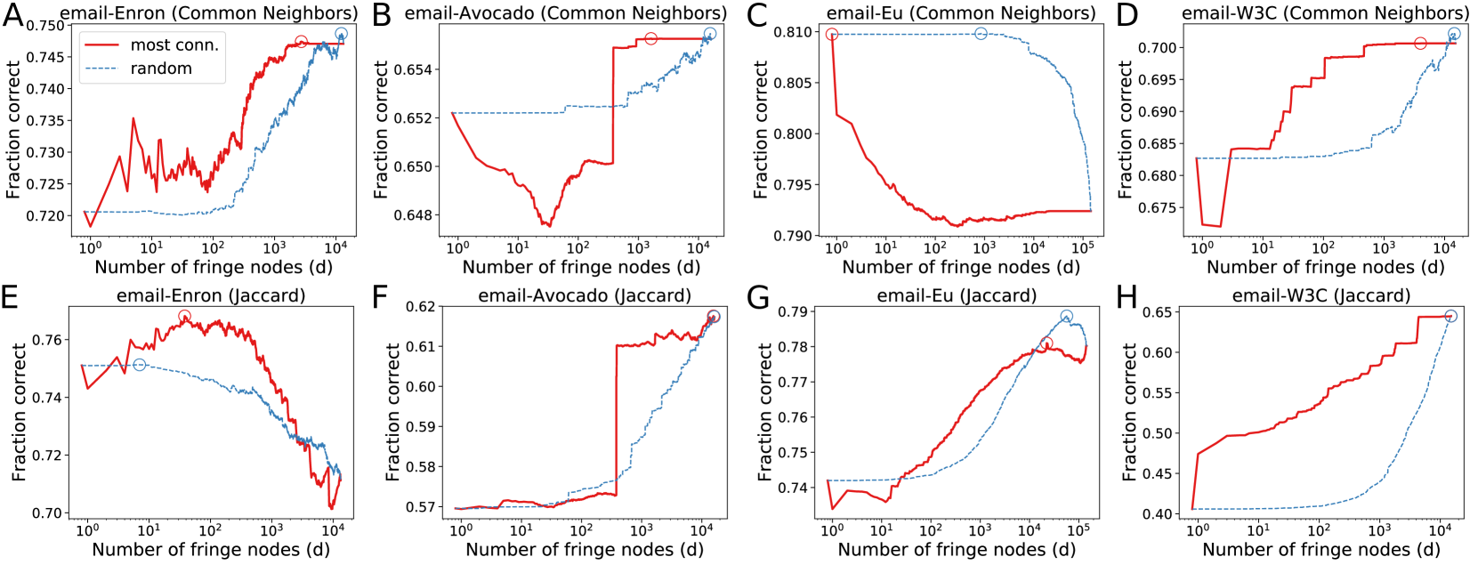
Figure 2. Link prediction performance of the Common Neighbors (top) and Jaccard similarity (bottom) score functions on four email networks as a function of $d$, the number of fringe nodes included. Two orderings of fringe nodes are considered: one by the most connections to the core (red) and one random (blue). A circle marks the best performance. There is a striking variety in how the fringe affects performance. In some cases, we should ignore the fringe entirely (C); in others, performance increases with the size of the fringe (F, H); and in still others, some intermediate amount of fringe is optimal (E, G).

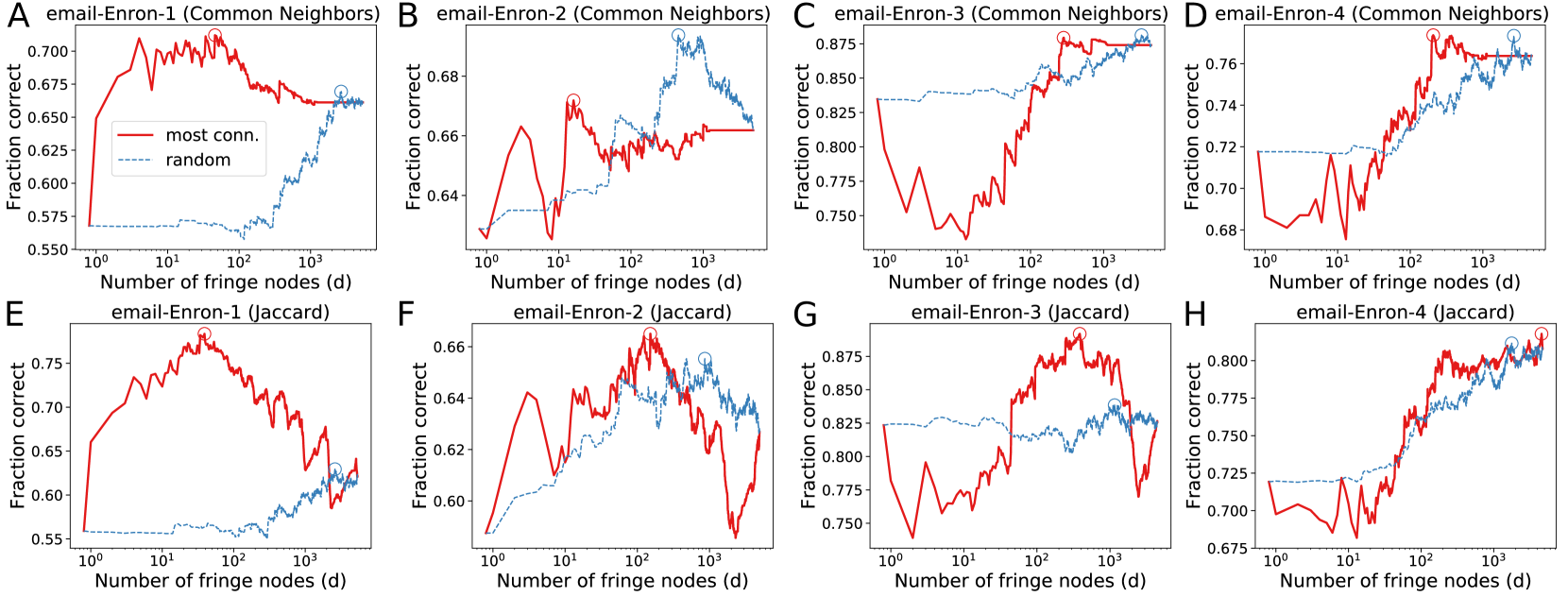
Figure 3. Link prediction performance experiments analogous to those in Figure 2 but on four subsets of email-Enron. In most cases, including some interior amount of fringe nodes—between 10 and a few hundred—yields the optimal performance.

Our first set of experiments analyzes email networks. The core nodes in these datasets are members of some organization, and the fringe nodes are those outside of the organization that communicate with those in the core. We use four email networks; in each, the nodes are email addresses, and the time that an edge formed is given by the timestamp of the first email between two nodes. For simplicity, we consider all graphs to be undirected, even though there is natural directionality in the links. Thus, each dataset is a simple, undirected graph, where each edge has a timestamp and each node is labeled as core or fringe. The four datasets are (i) email-Enron: the network in Figure 1, where the core nodes correspond to accounts whose emails were released as part of a federal investigation (Klimt and Yang, 2004; Benson and Kleinberg, 2018); (ii) email-Avocado: the email network of a now-defunct company, where the core nodes are employees (we removed accounts associated with non-people, such as conference rooms). (iii) email-Eu: a network that consists of emails involving members of a European research institution, where the core nodes are the institution’s members (Leskovec et al., 2007; Yin et al., 2017); and (iv) email-W3C: a network from W3C email threads, where core nodes are those addresses with a w3.org domain (Craswell et al., 2005; Benson and Kleinberg, 2018). Table 1 provides basic summary statistics.

An entire email network dataset is a graph $G=(V,E)$, where $C\subseteq V$ is a set of core nodes, and each edge $e\in E$ is associated with a timestamp $t_{e}$. Here, our test set is derived from the temporal information. Let $t^{*}$ be the 80th percentile of timestamps on edges between core nodes. Our test set of edges is the final 20% of edges between core nodes that appear in the dataset:

(5) $$E^{\textnormal{test}}=\{(u,v)\in E\;|\;u,v\in C\text{ and }t_{(u,v)}\geq t^{*}\}.$$

The training set is then given by edges appearing before $t^{*}$, i.e., the edges appearing in the first 80% of time spanned by the data:

(6) $$E^{\textnormal{train}}=\{(u,v)\in E\;|\;t_{(u,v)}<t^{*}\}.$$

Fringe ordering.  Next, we form the nested sequence of training set edges (Eq. 4) by sequentially increasing the amount of fringe information (Eq. 3). Recall that $E_{d}^{\textnormal{train}}$ is simply the set of edges in $E^{\textnormal{train}}$ in which both end points are in the vertex set $V_{d}$. To build $\{V_{d}\}$, we start with $V_{0}=C$, the core set, and then add the fringe nodes one by one in order of decreasing degree in the graph $G^{\textnormal{train}}=(V,E^{\textnormal{train}})$. By definition, fringe nodes cannot link between themselves, so this ordering is equivalent to adding fringe nodes in order of the number of core nodes to which they connect. For purposes of comparison, we also evaluate this ordering relative to a uniformly random ordering of the fringe nodes. To summarize, given an ordering $\sigma$ of the fringe nodes $F$, we create a nested sequence of node sets $V_{d}=C\cup\{\sigma_{1},\ldots,\sigma_{d}\}$ in two ways: (i) Most connected: $\sigma$ is the ordering of nodes in the fringe $F$ by decreasing degree in the graph induced by $E^{\textnormal{train}}$ (Eq. 6); and (ii) Random: $\sigma$ is a random ordering of the nodes in $F$.

Link prediction.  We use the most connected and random ordering to predict links in the test set of edges, as described at the beginning of Section 2. Recall that we needed a set of candidate comparisons between two potential edges (one of which does appear in the test). We guess that the pair of nodes with the larger number of common neighbors or larger Jaccard similarity score will be the set that appears in the test set. We sample $10\cdot\lvert E^{\textnormal{test}}\rvert$ pairs from $E^{\textnormal{test}}$ (allowing for repeats) and combine each of them with two nodes selected uniformly at random that never form an edge. Prediction performance is measured in terms of the fraction of correct guesses as a function of $d$, the number of fringe nodes included. This entire procedure is repeated 10 times (with 10 different sets of random samples) and the mean accuracy is reported in Figure 2.

The results exhibit a wide variety of behavior. In some cases, performance tends to increase monotonically with the number of fringe nodes (Figures 2 and 2). In one case, we achieve optimal performance by ignoring the fringe entirely (Figure 2). In yet another case, some interior amount of fringe is optimal before prediction performance degrades (Figure 2). In several cases, we see a saturation effect, where performance flattens as we increase more fringe nodes (e.g., Figures 2 and 2). This is partly a consequence of how we ordered the fringe—nodes included towards the end of the sequence are less connected and thus have relatively less impact on the score functions. In these cases, one practical consequence is that we could ignore large amounts of the data and get roughly the same performance, which would save computation time. In another case, the first few hundred most connected fringe nodes leads to worse performance, but eventually having enough fringe improves performance (Figure 2). Finally, there are also cases where the optimal performance over $d$ is better for a random ordering of the fringe than for the most connected ordering (Figures 2 and 2).

We repeated the same set of experiments on subgraphs of email-Enron by partitioning the core set of nodes $C$ into four groups to induce four different datasets. In each dataset, the other members of the core are removed from the graph entirely (the bottom part of Table 1 lists basic summary statistics). The results in Figure 3 provide further evidence that it is a priori unclear how much fringe information one should include to achieve the best performance. In nearly all cases, the optimal performance when including fringe nodes in order of connectedness is somewhere between 10 and a few hundred nodes, out of a total of several thousand. And we again see that including initial fringe information by connectedness has worse performance than ignoring the fringe entirely, until eventually incorporating enough fringe information provides enough signal to improve prediction performance (Figures 3 and 3).

2.2. Telecommunications networks

Table 2. Summary statistics of telecommunications datasets. Core nodes are participants in the Reality Mining study.

	# core	# fringe	# core-core	# core-fringe
Dataset	nodes	nodes	edges	edges
call-Reality	91	8,927	127	10,512
text-Reality	91	1,087	32	1,920

Next, we study telecommunications datasets from cell phone usage amongst individuals participating in the Reality Mining project (Eagle and Pentland, 2005). This project recorded cell phone activity of students and faculty in the MIT Media Laboratory, including calls and SMS texts between phone numbers. We consider the participants (more, specifically, their phone numbers) as the core nodes in our network. Edges are phone calls or SMS texts between two people, some of which are fringe nodes corresponding to people who were not recruited for the experiment. We process the data in the same way as for email networks—directionality was removed and the edges are accompanied by the earliest timestamp of communication between the two nodes. We study two datasets: (i) call-Reality: the network of phone calls (Eagle and Pentland, 2005; Benson and Kleinberg, 2018); and (ii) text-Reality: the network of SMS texts (Eagle and Pentland, 2005; Benson and Kleinberg, 2018). Table 2 provides some basic summary statistics.

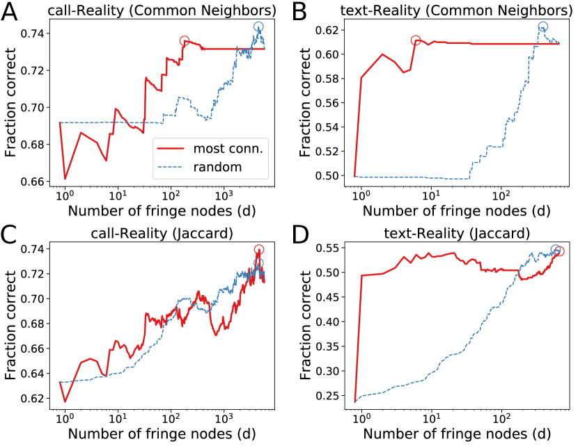
Figure 4. Link prediction performance in the telecommunications datasets as a function of $d$, the number of fringe nodes used for prediction. Circles mark the largest value. With the Common Neighbors score function, a small number of fringe nodes is optimal for these datasets.

Fringe ordering.  The structure of these networks is the same as the email networks—the dataset is a recording of the interactions of a small set of core nodes with a larger set of fringe nodes. We use the same two orderings—most connected to core and random—as we did for the email datasets. Thus, the nested sequence of node sets $\{V_{d}\}$ is again constructed by adding one node at a time.

Link prediction.  Figure 4 shows the link prediction performance on the telecommunications datasets. With the Common Neighbors score function, we again find that the optimal amount of fringe is a small fraction of the entire dataset—around 100 of nearly 9,000 nodes in call-Reality (Figure 4) and around 10 of over 1,000 nodes in text-Reality (Figure 4). The performance of the Jaccard similarity also has an interior optimum for the call-Reality dataset, although the optimum size here is larger—around half of the nodes.

Prediction performance with the fringe nodes ordered by connectedness to the core is in general quite erratic for the call-Reality dataset. This is additional evidence that the fringe nodes can be a noisy source of information. For instance, just including the first fringe node results in a noticeable drop in prediction performance for both the Common Neighbors and Jaccard score functions.

2.3. Online social networks

Table 3. Summary statistics of LiveJournal networks. The sets of core nodes are users in particular states or counties.

	# core	# fringe	# core-core	# core-fringe
Dataset	nodes	nodes	edges	edges
Wisconsin	16,842	58,965	48,078	87,723
Texas	65,617	155,357	256,174	312,746
New York	82,275	208,516	281,981	477,845
California	152,171	244,605	712,803	722,835
Marathon	223	1,032	390	1,363
Eau Claire	295	1,392	252	1,635
Dane	2,281	15,580	5,192	21,156
Milwaukee	3,743	19,934	10,750	30,955

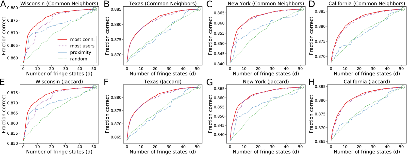
Figure 5. Link prediction performance of the Common Neighbors (top) and Jaccard similarity (bottom) score functions on four LiveJournal datasets where the core consists of users in a state. Performance is measured as a function of $d$, the number of fringe states included for prediction (for four different orderings of the fringe). The most connected ordering performs the best, monotonically increases with $d$, and saturates when $d\geq 20$.

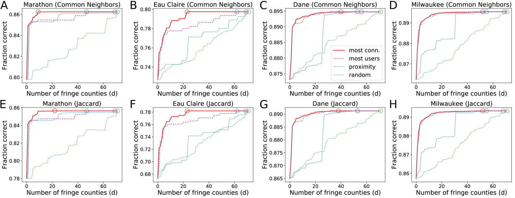
Figure 6. Link prediction analogous to Figure 5 but where the core is a Wisconsin county and the fringe is the rest of the state. Performance is measured as a function of $d$, the number of fringe counties included for prediction. The most connected ordering performs the best, and performance with this ordering quickly saturates.

We now turn to links in an online social network of bloggers from the LiveJournal community (Liben-Nowell et al., 2005). Edges are derived from users listing friends in their profile (here, we consider all links as undirected). Users also list their geographic location, and for the purposes of this study, we have restricted the dataset to users reporting locations in the United States and Puerto Rico. For each user, we have both their territory of residence (one of the 50 U.S. states, Washington D.C., or Puerto Rico; henceforth simply referred to as “state”) as well as their county of residence, when applicable.

We construct core-fringe networks in two ways. First, we form a core from all user residing in a given state $S$. The core-fringe network then consists of all friendships where at least one node is in state $S$. We construct four such networks, using the states Wisconsin, Texas, California, and New York. Second, we form a core from users residing in a county and construct a core-fringe network in the same way, but we only consider friendships amongst users in the state containing the county. We construct four such networks, using Marathon, Eau Claire, Dane, and Milwaukee counties (all in Wisconsin). Table 3 lists summary statistics of the datasets.

Unlike the email and telecommunications networks, we do not have timestamps on the edges. We instead construct $E^{\textnormal{test}}$ from a random sample of 20% of the edges between core nodes, i.e., from $\{(u,v)\in E\;|\;u,v\in C\}$, and set $E^{\textnormal{train}}=E-E^{\textnormal{test}}$. Predicting on such held out test sets is used for predicting missing links (Clauset et al., 2008; Ghasemian et al., 2018); here, we use it for link prediction, as is standard practice (Lü and Zhou, 2011).

Fringe ordering.  We again incorporate fringe nodes from a nested sequence of node sets $\{V_{d}\}$, where $V_{d}\subseteq V_{d+1}$ and $V_{0}=C$, the set of core nodes. The nested sequence of training sets is then $E_{d}^{\textnormal{train}}=\{(u,v)\in E^{\textnormal{train}}\;|\;u,v\in V_{d}\}$. With email and telecommunications, we considered fringe nodes one by one to form the sequence $\{V_{d}\}$. For LiveJournal, each successive node set instead corresponds to adding all nodes in a state or a county. For the cores constructed from users in a state (Wisconsin, Texas, New York, or California), we form orderings $\sigma$ of the remaining states in four ways: (i) Most connected: $\sigma$ is the ordering of states by decreasing number of links to the core state; (ii) Most users: $\sigma$ is the ordering by decreasing number of users; (iii) Proximity: $\sigma$ is the ordering of states by closest proximity to the core state (measured by great-circle distance between geographic centers); and (iv) Random: $\sigma$ is a random ordering of the states.

Let $U_{S}$ be the users in state $S$. The sequence of vertex sets is all users in the core and first $d$ states in the ordering $\sigma$. Formally, $V_{d}=C\phantom{!}\cup\phantom{!}(\cup_{t=1}^{d}U_{\sigma_{t}})$. For networks whose core are users in a Wisconsin county, we use the same orderings, except we order counties instead of states and the fringe is only counties in Wisconsin.

Link prediction.  We measure the mean prediction performance over 10 random trials as a function of the number $d$ of fringe states or counties included in the training data. When states form the core, prediction performance is largely consistent (Figure 5). For both score functions, ordering by number of connections tends to perform the best, with a rapid performance increase from approximately the first 10 states and then saturation with a slow monotonic increase. The prediction by states with the most users performs nearly the same for the three largest states (Texas, New York, and California; Figures 5, 5 and 5). In Wisconsin and New York, ordering by proximity shows a steep rise in performance for the first few states but then levels off (Figures 5, 5, 5 and 5). On the other hand, in California and Texas, ordering by proximity performs roughly as well as a random ordering.

The networks where the cores are users from counties in Wisconsin have similar characteristics to the networks where the cores are users from particular states (Figure 6). The ordering by county with the most connections performs the best. Prediction performance quickly saturates in the two larger counties (Figures 6 and 6), and the proximity ordering can be good in some cases (Figure 6).

Summary.  Usually, collecting additional data is thought to improve performance in machine learning. Here we have seen that this is not the case in some networks with core-fringe structure. In fact, including additional fringe information can affect link prediction performance in a number of ways. In some cases, it is indeed true that additional fringe always helps, which was largely the case with LiveJournal (Figure 5). In one email network, including any fringe data hurt performance (Figure 2). And yet in other cases, some intermediate amount of fringe data gave the best performance (Figures 4 and 4; Figure 3). We also observed saturation in link prediction performance as we increased the fringe size (Figure 6) and that sometimes we need enough fringe before prediction becomes better than incorporating no fringe at all (Figures 2 and 3). While this landscape is complex, we show in the next section how these behaviors can emerge in simple random graph models.

3. Random graph model analysis

We now turn to the question of why link prediction in core-fringe networks exhibits such a wide variation in performance. To gain insight into this question, we analyze the link prediction problem on basic random graph models that have been adapted to contain core-fringe structure.

Recall how our link prediction problem is evaluated: we are given two pairs $\{u,v\}$ and $\{w,z\}$; our algorithm predicts which of the two candidate edges is the one that appears in the data through a score function; and the values of the score function (and hence the predictions) can change based on the inclusion of fringe nodes. In a random graph model, we can think about using the same score functions for the candidate edges $(u,v)$ and $(w,z)$, but now the score functions and the existence of edges are random variables. As we will show, the signal-to-noise ratio of the difference in score functions is a key statistic to optimize in order to make the most accurate predictions, and this can vary in different ways when including fringe nodes.

The signal-to-noise ratio (SNR).  Suppose our data is generated by a random graph model and that the indicator random variables $X,Y\in\{0,1\}$ correspond to the existence of two candidate edges $\{u,v\}$ and $\{w,z\}$, respectively, where nodes $u$, $v$, $w$, and $z$ are distinct and chosen uniformly at random amongst a set of core nodes. Without loss of generality, we assume that $\textnormal{Pr}[X]>\textnormal{Pr}[Y]$ so that $(u,v)$ is more likely to appear.

We would like our algorithm to predict that the edge $\{u,v\}$ is the one that exists, since this is the more likely edge (by assumption). However, our algorithm does not observe $X$ and $Y$ directly; instead, it sees proxy measurements $(\hat{X},\hat{Y})$, which are themselves random variables. These proxy measurements correspond to the score function used by the algorithm; in this section, we focus on the number of common neighbors score. Our algorithm will (correctly) predict that edge $\{u,v\}$ is more likely if and only if $\hat{X}>\hat{Y}$.

Furthermore, the proxy measurements are parameterized by the amount of fringe information we have. Following our previous notation, we call these random variables $\hat{X}_{d}$ and $\hat{Y}_{d}$. These variables represent the same measurements as $\hat{X}$ and $\hat{Y}$ (such as the number of common neighbors), just on a set of graphs parameterized by the amount of fringe information $d$.

Our goal is to optimize the amount of fringe to get the most accurate predictions. Formally, if we let $Z_{d}\triangleq\hat{X}_{d}-\hat{Y}_{d}$, this means:

$$\textstyle\underset{d}{\text{maximize}}\quad\textnormal{Pr}[\hat{X}_{d}>\hat{Y}_{d}]\iff\underset{d}{\text{maximize}}\quad\textnormal{Pr}[Z_{d}>0].$$

We assume that we have access to $\mathbb{E}[Z_{d}]$ and $\mathbb{V}[Z_{d}]$ for all values of $d$. Our approach will be to maximize the signal-to-noise ratio (SNR) statistic of $Z_{d}$, i.e.,

$$\textstyle\underset{d}{\text{maximize}}\quad\frac{\mathbb{E}[Z_{d}]}{\sqrt{\mathbb{V}[Z_{d}]}}\triangleq\textnormal{SNR}[Z_{d}].$$

We motivate this approach as follows. Absent any additional information beyond the expectation and variance, we must use some concentration inequality. Under the reasonable assumption that $\mathbb{E}[Z_{d}]>0$ (which we later show holds in our models), the proper inequality is Cantelli’s: $\textnormal{Pr}[Z_{d}\geq 0]\geq 1-\frac{\mathbb{V}[Z_{d}]}{\mathbb{V}[Z_{d}]+\mathbb{E}[Z_{d}]^{2}}=\frac{\textnormal{SNR}[Z_{d}]^{2}}{1+\textnormal{SNR}[Z_{d}]^{2}}$. Thus, the lower bound on correctly choosing $X$ is monotonically increasing in the SNR of our proxy measurement. Using this probabilistic framework, we can now see how some of the empirical behaviors in Section 2 might arise.

3.1. Stochastic block models

In the stochastic block model, the nodes are partitioned into $K$ blocks, and for parameters $P_{i,j}$ (with $1\leq i,j\leq K$), each node in block $i$ is connected to each node in block $j$ independently with probability $P_{i,j}$. (Since our graphs are undirected, $P_{i,j}=P_{j,i}$.) In our core-fringe model here, $K=4$, the core corresponds to blocks $1$ and $2$, and the fringe corresponds to blocks $3$ and $4$. This model turns out to be flexible enough to demonstrate a wide range of behaviors observed in Section 2. We use the following notation for block probabilities:

(7) $$P=\begin{bmatrix}p&q&r&s\\ q&p&s&r\\ r&s&0&0\\ s&r&0&0\\ \end{bmatrix}.$$

Our assumptions on the probabilities are that $q<p$ and $s\leq r$. We also assume that the first two blocks each contain $n_{c}$ nodes and that the last two blocks each contain $n_{f}$ nodes.

We further assume we are given samples of four distinct nodes $u$, $v$, $w$, and $z$ chosen uniformly at random from the core blocks such that $u$, $v$, and $w$ are in block 1 and $z$ is in block 2. Following our notation above, let $X$ be the random variable that $(u,v)$ is an edge and $Y$ be the random variable that $(w,z)$ is an edge ($\textnormal{Pr}[X]>\textnormal{Pr}[Y]$ since $p>q$). Our proxy measurements $\hat{X}$ and $\hat{Y}$ are the number of common neighbors of candidate edges $\{u,v\}$ and $\{w,z\}$. Our algorithm will correctly predict that $(u,v)$ is more likely if $\hat{X}>\hat{Y}$.

Our proxy measurements are parameterized by the amount of fringe information that they incorporate. Here, we arbitrarily order the nodes in the two equi-sized fringe blocks and say that the random variable $\hat{X}_{d}$ is the number of common neighbors between nodes $u$ and $v$ when including the first $d$ nodes in both fringe blocks. Similarly, the random variable $\hat{Y}_{d}$ is the number of common neighbors of nodes $w$ and $z$. By independence of the edge probabilities, some straightforward calculations show that

$$\mathbb{E}[\hat{X}_{d}] =2(n_{c}-1)p^{2}+dr^{2}+ds^{2},\;\mathbb{E}[\hat{Y}_{d}]=2(n_{c}-1)pq+2drs$$

$$\mathbb{V}[\hat{X}_{d}] =2(n_{c}-1)p^{2}(1-p^{2})+dr^{2}(1-r^{2})+ds^{2}(1-s^{2})$$

$$\mathbb{V}[\hat{Y}_{d}] =2(n_{c}-1)pq(1-pq)+2drs(1-rs).$$

With no fringe information, it is immediate that the SNR is positive, i.e., $\textnormal{SNR}[Z_{0}]>0$: $\mathbb{E}[\hat{X}_{0}-\hat{Y}_{0}]=2(n_{c}-1)p[p-q]>0$ as $p>q$. If the two fringe blocks connect to the two core blocks with equal probability, then the SNR with no fringe is optimal.

Lemma 3.1 (No-fringe optimality).

If $r=s$ in the core-fringe SBM, then $\textnormal{SNR}[Z_{d}]$ decreases monotonically in $d$.

Proof.

When $r=s$, by independence of $\hat{X}_{d}$ and $\hat{Y}_{d}$,

$$\mathbb{E}[Z_{0}]=\mathbb{E}[\hat{X}_{d}-\hat{Y}_{d}] =2(n_{c}-1)p^{2}+dr^{2}+ds^{2}-2(n_{c}-1)pq-2drs$$

$$=2(n_{c}-1)p^{2}-2(n_{c}-1)pq=\mathbb{E}[\hat{X}_{0}-\hat{Y}_{0}],$$

and $\mathbb{V}[Z_{d}]=\mathbb{V}[\hat{X}_{d}]+\mathbb{V}[\hat{Y}_{d}]>\mathbb{V}[\hat{X}_{0}]+\mathbb{V}[\hat{Y}_{0}]=\mathbb{V}[Z_{0}]$. ∎

This result is intuitive. If the two fringe blocks connect to the core nodes with equal probability, then the node pairs $(u,v)$ and $(w,z)$ receive additional extra common neighbors according to exactly the same distributions. Thus, these fringe nodes provide noise but no signal. We confirm this result numerically with parameter settings $p=0.5$, $q=0.3$, $s=r=0.2$, and $n_{c}=10$ (Figure 7). Indeed, the SNR monotonically decreases as we include more fringe.

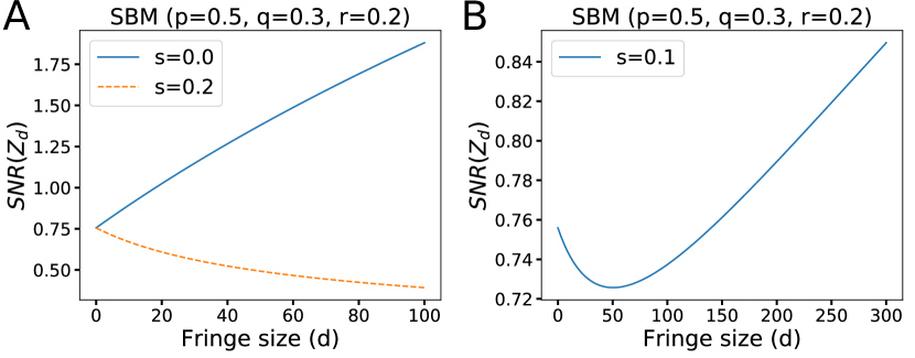
Figure 7. SNR for the difference in the common neighbors in our stochastic block model of core-fringe structure with $n_{c}=10$. (A) When the fringe blocks have equal probability of connecting to the two core blocks ($r=s$), the SNR decreases monotonically with fringe size by Lemma 3.1. When fringe blocks only connect to one of the core blocks ($s=0.0$), the SNR increases monotonically with fringe size Lemma 3.2. (B) For an intermediate parameter setting, including the fringe hurts the SNR until enough fringe is included, at which point the SNR increases monotonically (Lemma 3.3).

In Section 2, we saw cases where including any additional fringe information always helped. The following lemma shows that we can set parameters in our core-fringe SBM such that including any additional fringe information always increases the SNR.

Lemma 3.2 (All-fringe optimality).

Let $r>0$, $s=0$ and $4(n_{c}-1)(p^{2}-p^{4})>1$ in the core-fringe SBM. Then $\textnormal{SNR}[Z_{d}]$ monotonically increases in $d$ and $\lim_{d\to\infty}\textnormal{SNR}[Z_{d}]=\infty$.

Proof.

We have that

$$\textstyle\textnormal{SNR}[Z_{d}]=\frac{2(n_{c}-1)p(p-q)+dr^{2}}{\sqrt{2(n_{c}-1)(p^{2}(1-p^{2})+pq(1-pq))+dr^{2}(1-r^{2})}}.$$

We can treat this function as continuous in $d$. Then

$$\textstyle\lim_{d\to\infty}\textnormal{SNR}[Z_{d}]=\lim_{d\to\infty}\frac{dr^{2}}{\sqrt{dr^{2}(1-r^{2})}}=\infty.$$

Similarly, we can compute the derivative with respect to $d$:

$$\textstyle\frac{\partial}{\partial d}\textnormal{SNR}[Z_{d}]=\frac{r^{2}\sqrt{\mathbb{V}[Z_{d}]}-\frac{1}{2}r^{2}(1-r^{2})/\sqrt{\mathbb{V}[Z_{d}]}}{\mathbb{V}[Z_{d}]}$$

The derivative is positive provided that $r^{2}\mathbb{V}[Z_{d}]>\frac{1}{2}r^{2}(1-r^{2})$, which is true if $\mathbb{V}[Z_{0}]>\frac{1}{2}$ since $\mathbb{V}[Z_{0}]$ is monotonically increasing in $d$. We have that

$$\mathbb{V}[Z_{0}]=2(n_{c}-1)(p^{2}(1-p^{2})+pq(1-pq))>2(n_{c}-1)(p^{2}-p^{4}).$$

Thus, the result holds provided $4(n_{c}-1)(p^{2}-p^{4})>1$. ∎

The result is again intuitive. By setting $s=0$, the pair of nodes in different blocks ($w$ and $z$) get no additional common neighbors from the fringe, whereas the pair of nodes in the same block ($u$ and $v$) get additional common neighbors. This should only help our prediction performance, which is why the SNR monotonically increases. We confirm this result numerically (Figure 7), where we use the same parameters as the experiment described above. We can also check that the conditions of Lemma 3.2 are met: $n_{c}=10$ and $p=0.5$, so $4(n_{c}-1)(p^{2}-p^{4})=6.75>1$.

The SBM can also exhibit additional behaviors that we observed in Section 2. For example, with the email-Enron-4 dataset, prediction performance initially decreased as we included more fringe and then began to increase (Figures 3 and 3). The following lemma says that the core-fringe SBM can capture this behavior.

Lemma 3.3 (Enough-fringe optimality).

Let $p$, $q$, and $r$ be given. Then there exists a value of $s$ in the core-fringe SBM such that $\textnormal{SNR}[Z_{d}]$ initially decreases and then increases without bound.

Proof.

To simplify notation, consider the following constants: $\alpha=\mathbb{E}[Z_{0}]=2(n_{c}-1)(p^{2}-pq)$, $\beta=(r-s)^{2}$, $\gamma=\mathbb{V}[Z_{0}]=2(n_{c}-1)[p^{2}(1-p^{2})+pq(1-pq)]$, and $\delta=r^{2}(1-r^{2})+s^{2}(1-s^{2})+2rs(1-rs)$. With this notation, $\textnormal{SNR}[Z_{d}]=(\alpha+\beta d)/\sqrt{\gamma+\delta d}$. Treating this as a continuous function in $d$, the derivative is: $\frac{\partial}{\partial d}\textnormal{SNR}[Z_{d}]=(-\alpha\delta+2\beta\gamma+\beta\delta d)/(2(\gamma+\delta d)^{3/2})$. For any $s$, we can choose a sufficiently large $D$ such that the derivative is positive when $d>D$, meaning that $\textnormal{SNR}[Z_{d}]$ is increasing. Furthermore, $\textnormal{SNR}[Z_{d}]$ grows as $O(\sqrt{d})$. It is easy to check that the derivative also has at most one root, $d_{0}=\alpha/\beta-2\gamma/\delta$. We claim that $d_{0}$ can be made as large as desired. By setting $s$ sufficiently close to $r$, $\beta$ approaches $0$, while $\delta$ is bounded away from $0$. The remaining terms are positive constants. Finally, when $d=0$, the value of the derivative is $(-\alpha\delta+2\beta\gamma)/(2\gamma^{3/2})$. Again, we can make $s$ sufficiently close to $r$ so that $\beta$ approaches $0$ and the derivative is negative at $d=0$. Therefore, there exists an $s$ such that its derivative has one root $d_{0}\geq 1$, $\textnormal{SNR}[Z_{d}]$ decreases for small enough $d$ and eventually increases without bound. ∎

By setting $n_{c}=10$, $p=0.5$, $q=0.3$, $r=0.2$, and $s=0.1$, we see the behavior described by Lemma 3.3—the SNR initially decreases with additional fringe but then increases monotonically (Figure 7).

By extending the SBM to include a third fringe block, we can also have a case where an intermediate amount of core is optimal. We argue informally as follows. We begin with a setup as in Lemma 3.2, where $s=0$. Including all of the fringe available in these blocks is optimal. We then add a third fringe block that connects with equal probability to the two core blocks. By the arguments in Lemma 3.1, this only hurts the SNR. Thus, it is optimal to include two of the three fringe blocks, which is an intermediate amount of fringe.

3.2. Small-world lattice models

In the one-dimensional small-world lattice model (Kleinberg, 2006), there is a node for each integer in $\mathbb{Z}$ and a parameter $\alpha\geq 0$. The probability that edge $(i,j)$ exists is

(8) $$\textstyle\textnormal{Pr}[(i,j)\in E]=\frac{1}{|j-i|^{\alpha}}.$$

We start with a core of size $2c+1$, centered around 0: $V_{0}=C=\{-c,\ldots,c\}$. We then sample two nodes $v$ and $w$ such that

(9) $$u=-c<v<w<c=z\text{ and }2\leq v-u<z-w.$$

In our language at the beginning of Section 3, $X$ is still the random variable that edge $(u,v)$ exists and $Y$ is the random variable that edge $(w,z)$ exists. By our assumptions and Eq. 8, we know that $\textnormal{Pr}[X]>\textnormal{Pr}[Y]$. However, we will again assume that we are only given access to the number of common neighbors through the proxy random variables $\hat{X}$ and $\hat{Y}$.

Our parameterization of the proxy measurements are a distance $d$ that we examine beyond the core. Specifically, the nested sequence of vertex sets that incorporate fringe information is given by $V_{d}=\{-(c+d),\ldots,c+d\}$, and our proxy measurements are

$$\hat{X}_{d} =\lvert\{s\in V_{d}\;|\;(u,s)\text{ and }(v,s)\text{ are edges}\}\rvert$$

$$\hat{Y}_{d} =\lvert\{s\in V_{d}\;|\;(w,s)\text{ and }(z,s)\text{ are edges}\}\rvert.$$

We will analyze the random variable $Z_{d}=\hat{X}_{d}-\hat{Y}_{d}$. We correctly predict that $(u,v)$ is more likely than $(w,z)$ to exist if $Z_{d}>0$. As argued above, our goal is to find a $d$ that maximizes $\textnormal{SNR}[Z_{d}]$.

We focus our analysis on the case of $\alpha=1$ in Eq. 8. Let $A_{s}$ be the indicator random variable that node $s$ is a common neighbor of nodes $u$ and $v$, for $s\in\mathbb{Z}\backslash\{u,v\}$, and let $B_{s}$ be the indicator random variable that node $s$ is a common neighbor of $w$ and $z$, for $s\in\mathbb{Z}\backslash\{w,z\}$. Since $u=-c$ and $z=c$, our proxy measurements are

(10) $$\hat{X}_{d} =\textstyle\sum_{s=-(c+d)}^{-(c+1)}A_{s}+\sum_{s=-c+1}^{v-1}A_{s}+\sum_{s=v+1}^{c+d}A_{s}$$

(11) $$\hat{Y}_{d} =\textstyle\sum_{s=-(c+d)}^{w-1}B_{s}+\sum_{s=w+1}^{c-1}B_{s}+\sum_{s=c+1}^{c+d}B_{s}$$

Define the independent indicator random variables $I_{s,r}$ and $J_{s,r}$ where $\textnormal{Pr}[I_{s,r}=1]=1/(s(s+r))$ and $\textnormal{Pr}[J_{s,r}=1]=1/(s(r-s))$. Now we can re-write the expressions for $\hat{X}_{d}$ and $\hat{Y}_{d}$ as follows:

(12) $$\hat{X}_{d} =\textstyle\sum_{s=1}^{d}I_{s,v-u}+\sum_{s=1}^{c+d-v}I_{s,v-u}+\sum_{s=1}^{v-u-1}J_{s,v-u}$$

(13) $$\hat{Y}_{d} =\textstyle\sum_{s=1}^{d}I_{s,z-w}+\sum_{s=1}^{w-c-d}I_{s,z-w}+\sum_{s=1}^{z-w-1}J_{s,z-w}.$$

The expectations are given by

$$\mathbb{E}[\hat{X}_{d}] =\textstyle\sum_{s=1}^{d}\frac{1}{s(s+v-u)}+\sum_{s=1}^{c+d-v}\frac{1}{s(s+v-u)}+\sum_{s=1}^{v-u-1}\frac{1}{s(v-u-s)}$$

$$\mathbb{E}[\hat{Y}_{d}] =\textstyle\sum_{s=1}^{d}\frac{1}{s(s+z-w)}+\sum_{s=1}^{w-c-d}\frac{1}{s(s+z-w)}+\sum_{s=1}^{z-w-1}\frac{1}{s(z-w-s)}.$$

With these expressions, we can now analyze how $Z_{d}$ behaves as we vary $d$. The following lemma establishes that $Z_{d}$ converges to a positive value. Later, we use this to show that the SNR also converges to a positive value.

Lemma 3.4.

$\lim_{d\to\infty}\mathbb{E}[Z_{d}]=Z^{*}>0$.

Proof.

Let $a=v-u$. Then $\lim_{d\to\infty}\mathbb{E}[\hat{X}_{d}]=2\sum_{s=1}^{\infty}\frac{1}{s(s+a)}+\sum_{s=1}^{a-1}\frac{1}{s(a-s)}=2(\psi(a+1)+\psi(a)+2\gamma)/a=2(2\psi(a)+1/a+2\gamma)/a$, where $\psi(\cdot)$ is the digamma function. Similarly, if $b=z-w$, then

$$\lim_{d\to\infty}\mathbb{E}[\hat{Y}_{d}]=2(2\psi(b)+1/b+2\gamma)/b.$$

Thus, $Z^{*}=\lim_{d\to\infty}\mathbb{E}[\hat{X}_{d}]-\mathbb{E}[\hat{Y}_{d}]$ exists, and $Z^{*}>0$ if and only if

(14) $$b(\psi(a)+1/(2a)+\gamma)-a(\psi(b)+1/(2b)+\gamma)>0$$

Recall that by Eq. 9, $2\leq a<b$. Numerically, Eq. 14 holds for $(a,b)=(2,3)$. Since the left-hand-side monotonically increases in $b$, this inequality holds for $a=2$.

Now assume $b>a\geq 3$. The Puiseux series expansion of $\psi$ at $\infty$ gives $\psi(x)+1/(2x)\in\log(x)\pm\frac{1}{12(x^{2}-1)}$. Thus, it is sufficient to show that $b(\log(a)-1/96)+(b-a)\gamma>a(\log(b)+1/180)$, or that $0.99b\log(a)+\gamma>1.01a\log(b)$, which holds for $b>a\geq 3$. ∎

The next theorem shows that the signal-to-noise ratio converges to a positive value. Thus, by measuring enough fringe, our proxy measurements are at least providing the correct direction of information. However, the SNR converges, so at some point, our information saturates.

Theorem 3.5 (SNR saturation).

$\lim_{d\to\infty}\textnormal{SNR}[Z_{d}]=S^{*}>0$.

Proof.

By Lemma 3.4, $\mathbb{E}[Z_{d}]$ converges to a positive value. Thus, it is sufficient to show that $\mathbb{V}[Z_{d}]$ converges. Following Eq. 12,

$$\textstyle\mathbb{V}[\sum_{s=1}^{\infty}I_{s,v-u}]=\textstyle\sum_{s=1}^{\infty}\mathbb{V}[I_{s,v-u}]=\textstyle\sum_{s=1}^{\infty}\frac{1}{s(s+v-u)}-\frac{1}{(s(s+v-u))^{2}}$$

by independence, and converges. ∎

The random variable $W_{d+1,J}\triangleq Z_{d+J}-Z_{d}=\sum_{k=d+1}^{k=d+1+J}I_{k,v-u}-I_{k,z-w}$ will be useful for our subsequent analysis. This is the additional measurement available to us if we measured at distance $d+J$ instead of $d$. The next lemma says that, as we increase $d$, the expectation of $W_{d,J}$ goes to zero faster than its variance.

Lemma 3.6.

For any $J$, $\lim_{d\to\infty}\mathbb{E}[W_{d,J}]/\mathbb{V}[W_{d,J}]=0$.

Proof.

Let $a=v-u$ and $b=z-w$. By independence,

$$\mathbb{E}[W_{d,J}] =\textstyle\sum_{k=d}^{k=d+J}\frac{1}{k(k+a)}-\frac{1}{k(k+b)}$$

$$=\textstyle\sum_{k=d}^{k=d+J}\frac{b-a}{k(k+a)(k+b)}=\textstyle O(\sum_{k=d}^{k=d+J}1/k^{3}).$$

For large enough $d$, $\mathbb{V}[W_{d,J}]=\textstyle\sum_{k=d}^{k=d+J}\frac{1}{k(k+a)}+\frac{1}{k(k+b)}-\frac{1}{(k(k+b))^{2}}-\frac{1}{(k(k+a))^{2}}$, which is $O(\sum_{k=d}^{k=d+J}1/k^{2})$. ∎

The next theorem now shows that in the one-dimensional lattice model, the signal-to-noise ratio eventually begins to decrease. This means that at some point, the noise overwhelms the signal. Thus, it will never be best to gather as much fringe as possible.

Theorem 3.7.

There exists a $D$ for which $\textnormal{SNR}[Z_{D}]>\textnormal{SNR}[Z_{D+j}]$ for any $j>0$.

Proof.

We have that $\textnormal{SNR}[Z_{d}]>\textnormal{SNR}[Z_{d+j}]$ if and only if

$$\textstyle\frac{\mathbb{E}[Z_{d}]}{\sqrt{\mathbb{V}[Z_{d}]}}>\frac{\mathbb{E}[Z_{d}+W_{d+1,j}]}{\sqrt{\mathbb{V}[Z_{d}+W_{d+1,j}]}} \iff\textstyle\frac{\mathbb{E}[Z_{d}]^{2}}{\mathbb{V}[Z_{d}]}>\frac{2\mathbb{E}[Z_{d}]\mathbb{E}[W_{d+1,j}]+\mathbb{E}[W_{d+1,j}]^{2}}{\mathbb{V}[W_{d+1,j}]}.$$

The second inequality above comes from squaring both sides of the first inequality; both terms in the first inequality are positive for large enough $d$ by Lemma 3.4, so we can keep the direction of the inequality. By Theorem 3.5, the left-hand-side of the inequality converges to a positive constant. We claim that the right-hand-side converges to $0$.

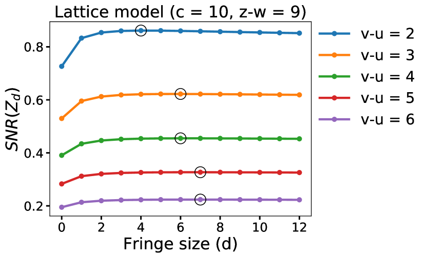
Figure 8. Saturation and interior optima of the SNR the one-dimensional small-world lattice model. Nodes $v$ and $w$ are sampled from $\{u=-c,\ldots,c=z\}$ with $2\leq v-u<z-w$. The random variable $Z_{d}$ is the difference in the number of common neighbors of $\{u,v\}$ and $\{w,z\}$ on the node set $\{-(c+d),\ldots,c+d\}$. Since $\textnormal{SNR}[Z_{1}]>\textnormal{SNR}[Z_{0}]$, an intermediate amount of fringe produces the optimal SNR (Corollary 3.8); these optima are circled in black. The SNR converges by Theorem 3.5, and we indeed see the consequent saturation.

By Lemma 3.4, $\mathbb{E}[Z_{d}]$ converges, so it must be bounded by a positive constant constant. Furthermore, since $Z_{d+j}=Z_{d}+W_{d+1,j}$, we have that $\mathbb{E}[W_{d+1,j}]\to 0$. Combining these results, $2\mathbb{E}[Z_{d}]\mathbb{E}[W_{d+1,j}]+\mathbb{E}[W_{d+1,j}]^{2}=O(\mathbb{E}[W_{d+1,j}])$, and we have that $\mathbb{E}[W_{d+1,j}]/\mathbb{V}[W_{d+1,j}]\to 0$ by Lemma 3.6. ∎

A consequence of this theorem is that if the SNR initially increases, then an intermediate amount of fringe is optimal. The reason is that the SNR initially increases but at some point begins to decrease monotonically (Theorem 3.7) before converging to a positive value (Theorem 3.5). We formalize this as follows.

Corollary 3.8 (Intermediate-fringe optimality).

If  $\textnormal{SNR}[Z_{0}]<\textnormal{SNR}[Z_{1}]$, then $d^{*}=\arg\max_{d}\textnormal{SNR}[Z_{d}]$ satisfies $0<d^{*}<\infty$.

Numerically, $\textnormal{SNR}[Z_{0}]<\textnormal{SNR}[Z_{1}]$ in several cases (Figure 8). In this experiment, we fix $c=10$ and $w=1$ (so $z-w=9$) and vary the amount of fringe from $0$ to $12$ nodes on either end of the core. We also vary $v$ so that $v-u\in\{2,3,4,5,6\}$. We observe two phenomena consistent with our theory. First, by Corollary 3.8, an intermediate amount of fringe information should be optimal; indeed, this is the case. Second, by Theorem 3.5, the SNR converges, indicating that saturation should kick in at some finite fringe size. This is true in our experiments, where saturation occurs after around $d=8$.

4. Discussion

Link prediction is a cornerstone problem in network science (Liben-Nowell and Kleinberg, 2007; Lü and Zhou, 2011), and the models for prediction include those that are mechanistic (Barabási et al., 2002), statistical (Clauset et al., 2008), or implicitly captured by a principled heuristic (Adamic and Adar, 2003; Backstrom and Leskovec, 2011). The major difference in our work is that we explicitly study the consequences of a common dataset collection process that results in core-fringe structure. Most related to our analysis of random graph models are theoretical justifications of principled heuristics such as the number of common neighbors in latent space models (Sarkar et al., 2011) and in general stochastic block models (Sarkar et al., 2015).

The core-fringe structure that we study can be interpreted as an extreme case of core-periphery structure in complex networks (Borgatti and Everett, 2000; Holme, 2005; Rombach et al., 2017; Zhang et al., 2015). In more classical social and economic network analysis, core-periphery structure is a consequence of differential status (Doreian, 1985; Laumann and Pappi, 1976). In this paper, the structure emerges from data collection mechanisms, which raises new research questions of the kind that we have addressed. However, our results hint that periphery nodes could also be noisy sources of information and possibly warrant omission in standard link prediction. Our fringe measurements can also be viewed as adding noisy training data, which is related to training data augmentation methods (Ratner et al., 2016; Ratner et al., 2017).

Conventional machine learning wisdom says that more data generally helps make better predictions. We showed that this is far from true in the common problem of network link prediction, where additional data comes from observing how some core set of nodes interacts with the rest of the world, inducing core-fringe structure. Our empirical results show that the inclusion of additional fringe information leads to substantial variability in prediction performance with common link prediction heuristics. We observed cases where fringe information is (i) always harmful, (ii) always beneficial, (iii) beneficial only up to a certain amount of collection, and (iv) beneficial only with enough collection.

At first glance, this variability seems difficult to characterize. However, we showed that these behaviors arise in some simple graph models—namely, the stochastic block model and the one-dimensional small-world lattice model—by interpreting the benefit of the fringe information as changing the signal-to-noise ratio in our prediction problem. Our datasets are certainly more complex than these models, but our analysis suggests that variability in prediction performance when incorporating fringe data is much more plausible than one might initially suspect. Even when fringe data is available in network analysis, we must be careful how we incorporate this data into the prediction models we build.

Data and software

The call-Reality, text-Reality, email-Enron, and email-W3C datasets, along with software for reproducing the results in this paper, are available at https://github.com/arbenson/cflp.

Acknowledgements

We thank David Liben-Nowell for access to the LiveJournal data and Jure Leskovec for access to the email-Eu data. This research was supported by NSF Awards DMS-1830274, CCF-1740822, and SES-1741441; a Simons Investigator Award; and ARO Award W911NF-19-1-0057.

References

- (1)
- Abbe (2018) Emmanuel Abbe. 2018. Community Detection and Stochastic Block Models: Recent Developments. Journal of Machine Learning Research 18, 177 (2018), 1–86. http://jmlr.org/papers/v18/16-480.html
- Abbe et al. (2016) Emmanuel Abbe, Afonso S. Bandeira, and Georgina Hall. 2016. Exact Recovery in the Stochastic Block Model. IEEE Transactions on Information Theory 62, 1 (2016), 471–487. https://doi.org/10.1109/tit.2015.2490670
- Adamic and Adar (2003) Lada A Adamic and Eytan Adar. 2003. Friends and neighbors on the web. Social networks 25, 3 (2003), 211–230.
- Backstrom and Leskovec (2011) Lars Backstrom and Jure Leskovec. 2011. Supervised Random Walks: Predicting and Recommending Links in Social Networks. In Proceedings of the Fourth ACM International Conference on Web Search and Data Mining. ACM, 635–644. https://doi.org/10.1145/1935826.1935914
- Barabási et al. (2002) A.L Barabási, H Jeong, Z Néda, E Ravasz, A Schubert, and T Vicsek. 2002. Evolution of the social network of scientific collaborations. Physica A: Statistical Mechanics and its Applications 311, 3-4 (2002), 590–614. https://doi.org/10.1016/s0378-4371(02)00736-7
- Benson and Kleinberg (2018) Austin R. Benson and Jon Kleinberg. 2018. Found Graph Data and Planted Vertex Covers. In Advances in Neural Information Processing Systems.
- Borgatti and Everett (2000) Stephen P Borgatti and Martin G Everett. 2000. Models of core/periphery structures. Social Networks 21, 4 (2000), 375–395. https://doi.org/10.1016/s0378-8733(99)00019-2
- Clauset et al. (2008) Aaron Clauset, Cristopher Moore, and M. E. J. Newman. 2008. Hierarchical structure and the prediction of missing links in networks. Nature 453, 7191 (2008).
- Craswell et al. (2005) Nick Craswell, Arjen P de Vries, and Ian Soboroff. 2005. Overview of the TREC 2005 Enterprise Track. In TREC, Vol. 5. 199–205.
- Decelle et al. (2011) Aurelien Decelle, Florent Krzakala, Cristopher Moore, and Lenka Zdeborová. 2011. Asymptotic analysis of the stochastic block model for modular networks and its algorithmic applications. Physical Review E 84, 6 (2011). https://doi.org/10.1103/physreve.84.066106
- Doreian (1985) Patrick Doreian. 1985. Structural equivalence in a psychology journal network. Journal of the American Society for Information Science 36, 6 (1985), 411–417. https://doi.org/10.1002/asi.4630360611
- Eagle and Pentland (2005) Nathan Eagle and Alex (Sandy) Pentland. 2005. Reality mining: sensing complex social systems. Personal and Ubiquitous Computing 10, 4 (2005), 255–268. https://doi.org/10.1007/s00779-005-0046-3
- Ghasemian et al. (2018) Amir Ghasemian, Homa Hosseinmardi, and Aaron Clauset. 2018. Evaluating overfit and underfit in models of network community structure. arXiv:1802.10582 (2018).
- Goel et al. (2013) Ashish Goel, Aneesh Sharma, Dong Wang, and Zhijun Yin. 2013. Discovering similar users on Twitter. In 11th Workshop on Mining and Learning with Graphs.
- Gupta et al. (2013) Pankaj Gupta, Ashish Goel, Jimmy Lin, Aneesh Sharma, Dong Wang, and Reza Zadeh. 2013. WTF: the who to follow service at Twitter. In Proceedings of the 22nd international conference on World Wide Web. ACM Press. https://doi.org/10.1145/2488388.2488433
- Holme (2005) Petter Holme. 2005. Core-periphery organization of complex networks. Physical Review E 72, 4 (2005). https://doi.org/10.1103/physreve.72.046111
- Kim and Leskovec (2011) Myunghwan Kim and Jure Leskovec. 2011. The Network Completion Problem: Inferring Missing Nodes and Edges in Networks. In Proceedings of the SIAM Conference on Data Mining. Society for Industrial and Applied Mathematics, 47–58. https://doi.org/10.1137/1.9781611972818.5
- Kleinberg (2006) Jon Kleinberg. 2006. Complex Networks and Decentralized Search Algorithms. In Proceedings of the International Congress of Mathematicians.
- Klimt and Yang (2004) Bryan Klimt and Yiming Yang. 2004. The Enron Corpus: A New Dataset for Email Classification Research. In Machine Learning: ECML 2004. Springer Berlin Heidelberg, 217–226. https://doi.org/10.1007/978-3-540-30115-8_22
- Kossinets (2006) Gueorgi Kossinets. 2006. Effects of missing data in social networks. Social Networks 28, 3 (2006), 247–268. https://doi.org/10.1016/j.socnet.2005.07.002
- Laumann et al. (1989) Edward O Laumann, Peter V Marsden, and David Prensky. 1989. The boundary specification problem in network analysis. Research methods in social network analysis 61 (1989), 87.
- Laumann and Pappi (1976) Edward O. Laumann and Franz U. Pappi. 1976. Networks of collective action: A perspective on community influence systems (Quantitative studies in social relations). Academic Press.
- Leskovec et al. (2007) Jure Leskovec, Jon Kleinberg, and Christos Faloutsos. 2007. Graph evolution: Densification and shrinking diameters. ACM Transactions on Knowledge Discovery from Data 1, 1 (2007), 2–es. https://doi.org/10.1145/1217299.1217301
- Liben-Nowell and Kleinberg (2007) David Liben-Nowell and Jon Kleinberg. 2007. The link-prediction problem for social networks. Journal of the American Society for Information Science and Technology 58, 7 (2007), 1019–1031. https://doi.org/10.1002/asi.20591
- Liben-Nowell et al. (2005) D. Liben-Nowell, J. Novak, R. Kumar, P. Raghavan, and A. Tomkins. 2005. Geographic routing in social networks. Proceedings of the National Academy of Sciences 102, 33 (aug 2005), 11623–11628. https://doi.org/10.1073/pnas.0503018102
- Lü and Zhou (2011) Linyuan Lü and Tao Zhou. 2011. Link prediction in complex networks: A survey. Physica A: Statistical Mechanics and its Applications 390, 6 (2011), 1150–1170. https://doi.org/10.1016/j.physa.2010.11.027
- Mossel et al. (2014) Elchanan Mossel, Joe Neeman, and Allan Sly. 2014. Belief propagation, robust reconstruction and optimal recovery of block models. In Conference on Learning Theory. 356–370.
- Rapoport (1953) Anatole Rapoport. 1953. Spread of information through a population with socio-structural bias I: Assumption of transitivity. Bulletin of Mathematical Biophysics 15, 4 (Dec. 1953), 523–533.
- Ratner et al. (2017) Alexander Ratner, Stephen H. Bach, Henry Ehrenberg, Jason Fries, Sen Wu, and Christopher Ré. 2017. Snorkel: rapid training data creation with weak supervision. Proceedings of the VLDB Endowment 11, 3 (2017), 269–282. https://doi.org/10.14778/3157794.3157797
- Ratner et al. (2016) Alexander J Ratner, Christopher M De Sa, Sen Wu, Daniel Selsam, and Christopher Ré. 2016. Data programming: Creating large training sets, quickly. In Advances in Neural Information Processing Systems. 3567–3575.
- Rombach et al. (2017) Puck Rombach, Mason A. Porter, James H. Fowler, and Peter J. Mucha. 2017. Core-Periphery Structure in Networks (Revisited). SIAM Rev. 59, 3 (2017), 619–646. https://doi.org/10.1137/17m1130046
- Romero et al. (2016) Daniel M. Romero, Brian Uzzi, and Jon M. Kleinberg. 2016. Social Networks Under Stress. In Proc. International World Wide Web Conference. 9–20. https://doi.org/10.1145/2872427.2883063
- Sarkar et al. (2015) Purnamrita Sarkar, Deepayan Chakrabarti, et al. 2015. The consistency of common neighbors for link prediction in stochastic blockmodels. In Advances in Neural Information Processing Systems. 3016–3024.
- Sarkar et al. (2011) Purnamrita Sarkar, Deepayan Chakrabarti, and Andrew W. Moore. 2011. Theoretical Justification of Popular Link Prediction Heuristics. In Proceedings of the Twenty-Second International Joint Conference on Artificial Intelligence. AAAI Press, 2722–2727. https://doi.org/10.5591/978-1-57735-516-8/IJCAI11-453
- Watts and Strogatz (1998) Duncan J. Watts and Steven H. Strogatz. 1998. Collective dynamics of ‘small-world’ networks. Nature 393 (1998), 440–442.
- Yin et al. (2017) Hao Yin, Austin R. Benson, Jure Leskovec, and David F. Gleich. 2017. Local Higher-Order Graph Clustering. In Proceedings of the 23rd ACM SIGKDD International Conference on Knowledge Discovery and Data Mining. ACM, 555–564. https://doi.org/10.1145/3097983.3098069
- Zhang et al. (2015) Xiao Zhang, Travis Martin, and M. E. J. Newman. 2015. Identification of core-periphery structure in networks. Physical Review E 91, 3 (2015). https://doi.org/10.1103/physreve.91.032803