Network-induced multistability: Lossy coupling and exotic solitary states

Abstract

The stability of synchronised networked systems is a multi-faceted challenge for many natural and technological fields, from cardiac and neuronal tissue pacemakers to power grids. In the latter case, the ongoing transition to distributed renewable energy sources is leading to a proliferation of dynamical actors. The desynchronization of a few or even one of those would likely result in a substantial blackout. Thus the dynamical stability of the synchronous state has become a focus of power grid research in recent years.

In this letter we uncover that the non-linear stability against large perturbations is dominated and threatened by the presence of solitary states in which individual actors desynchronise. Remarkably, when taking physical losses in the network into account, the back-reaction of the network induces new exotic solitary states in the individual actors, and the stability characteristics of the synchronous state are dramatically altered. These novel effects will have to be explicitly taken into account in the design of future power grids, and their existence poses a challenge for control.

While this letter focuses on power grids, the form of the coupling we explore here is generic, and the presence of new states is very robust. We thus strongly expect the results presented here to transfer to other systems of coupled heterogeneous Newtonian oscillators.

The power grid is a vast network connecting generators and consumers of electrical energy. Due to the ongoing energy transition, dynamical actors are becoming more numerous and heterogeneous, and new dynamical phenomena are expected to occur in future power grids. This has brought the dynamical stability of the necessary 50/60Hz synchronous state into sharp focus, and spurred a large number of theoretical works on this topic recently Dörfler et al. (2013); Dörfler and Bullo (2012); Motter et al. (2013); Schiffer et al. (2014, 2016); Rohden et al. (2012, 2014); Witthaut and Timme (2012). It is known that these oscillator networks can be multistable. Strong perturbations can move the power grid dynamics out of the basin of attraction of the synchronous state Menck et al. (2013, 2014); Hellmann et al. (2016); Mitra et al. (2017): synchrony collapses and blackout is the likely result.

The question of the stability of synchronisation is not specific to power grids, but is central to a wide range of systems, like coupled Josephson junctions and laser systems Larger et al. (2015); Wiesenfeld et al. (1998), animal and bacterial flocking behaviour Vicsek and Zafeiris (2012); Chen et al. (2017), Huygens’s pendulum clocks Bennett et al. (2002), crowd synchrony on London Millennium Bridge Abdulrehem and Ott (2009); Belykh et al. (2017) and chemical Tinsley et al. (2 09); Nkomo et al. (3 06) or mechanical oscillators Martens et al. (3 06); Kapitaniak et al. (5 05), as well as networks of neurons Herzog (2007).

In this letter we show that the non-linear dynamics of oscillators in power grids is fundamentally altered by the resistance of the lines (i.e. transfer conductances) and the resulting energy losses. The line resitances translate to a phase-lagged coupling as in the Kuramoto-Sakaguchi model Sakaguchi and Kuramoto (1986) which is a characteristic of most systems that can be described as coupled phase oscillators, e.g. by using a phase reduction approach Nakao (6 04). The presence of losses hence breaks the coupling symmetry and hampers a rigorous mathematical analysis, e.g. in terms of Lyapunov functions Chiang (1989); Tan et al. (1993). As a trade-off in favour of analysability, models are typically studied assuming a lossless regime, while less is known about the lossy case (e.g. Dörfler and Bullo (2012); Dörfler et al. (2013); Vu and Turitsyn (2015)).

In the following, we address how a lagged coupling alters the multistability of the system with a focus on possible pathways of desynchronisation. In particular we find that the presence of losses can vastly increase the likelihood that a random perturbation hits the basin of attraction of a solitary state. Some parameter regimes solely exhibiting synchronisation without losses become multistable in the presence of even minimal losses. We uncover novel solitary states with large basins that are qualitatively different to known, previously studied multistable states of the power grid. Remarkably, these effects appear in all parameter regimes and topologies studied. They seem to be completely robust, not relying on underlying symmetries.

It follows that, contrary to common belief in the community, losses are more important to be considered than expected. Purely network properties can fundamentally alter the dynamics of the oscillators in the system. Hence developing a detailed understanding of the non-linear network physics of power grids is of great practical importance going forward.

The research into the stability of the synchronous states of power grids in the theoretical physics and control engineering community is mainly performed using the Kuramoto model with inertia, also known as the swing equation, in which the phase $\phi_{i}$ of the complex voltage at the nodes is the dynamical variable. From engineering practice it is known that this equation accurately captures the short time behaviour of synchronous machines used today Weckesser et al. (3 08); Auer et al. (6 05), but it also serves as a fairly general starting point for the study of future control dynamics Schiffer et al. (2016). It accounts for a proportional response of the frequency to power imbalance and the presence of inertia, but neglects higher order internal dynamics as well as variations in the voltage magnitude. In the reference frame co-rotating with the synchronous frequency, the equations for $n$ nodes are given as:

$$H_{i}\ddot{\phi}_{i} =P_{i}-D_{i}\dot{\phi}_{i}-\sum\limits_{j=1}^{n}P_{ij}\;,$$ (1)

$$P_{ij} =K_{ij}\Biglb(\sin\left(\alpha_{ij}\right)+\sin\left(\phi_{i}-\phi_{j}-\alpha_{ij}\right)\Bigrb)\;.$$ (2)

Here $P_{i}$ is the power injected/consumed at node $i$, $D_{i}$ characterizes the power’s response to frequency changes, $H_{i}$ the inertia present and $P_{ij}$ is the power injected at node $i$ into the line connecting nodes $i$ and $j$. This power is given in terms of the phase difference and the complex admittance $Y_{ij}=-iK_{ij}\exp(i\alpha_{ij})$, with $K$ and $\alpha$ typically positive (see derivation in SI). This is the inverse of the complex impedance consisting of the reactance $X$ and the resistance $R$: $Y_{ij}=\frac{1}{R_{ij}+iX_{ij}}$. All quantities are in the per unit system, such that the voltage magnitude equals one. Typical parameter choices are discussed in the Methods section.

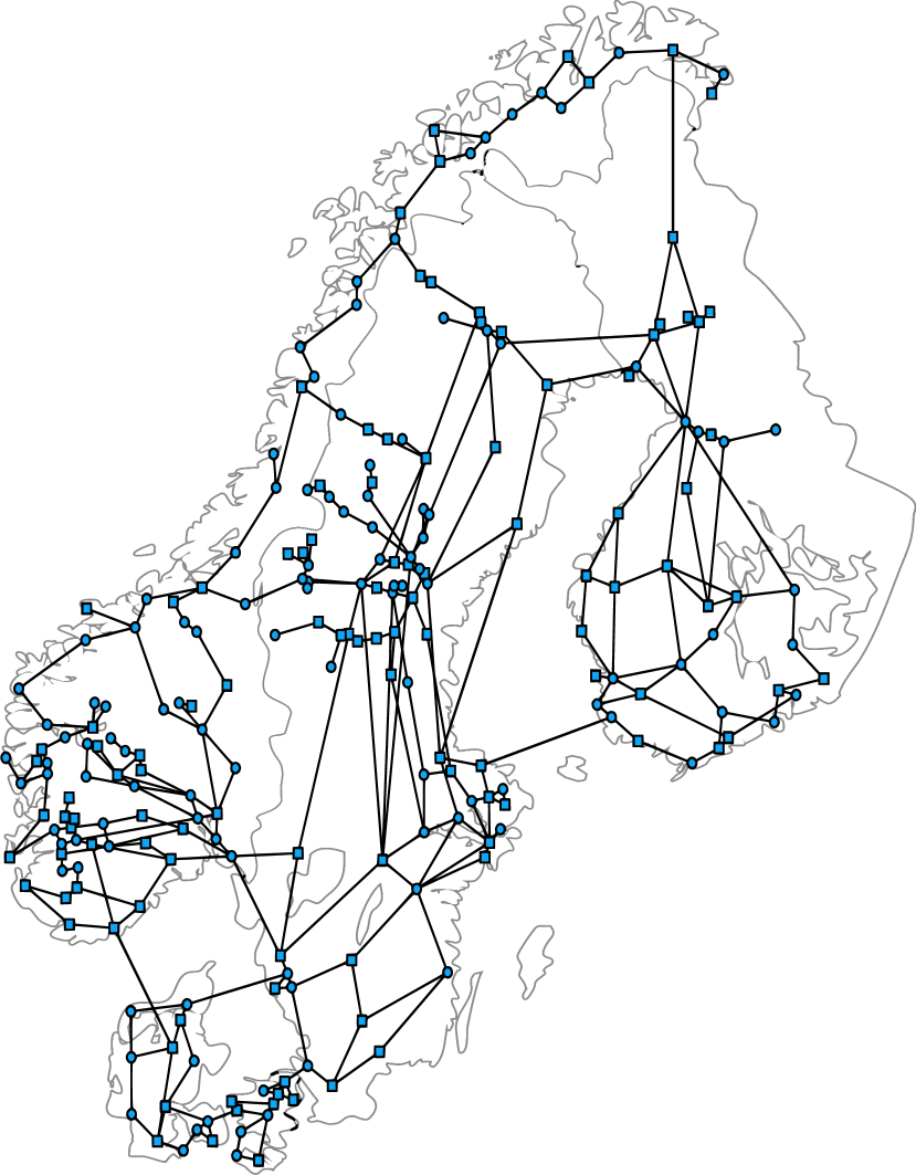
(a)

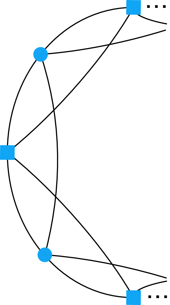
(b)

Figure 1: Network models. a The Scandinavian (extra-)high voltage transmission grid. b A circle topology with coupling to next-nearest neighbours, i.e. a coupling radius of $R=2$. In both cases, squares denote net consumers and circles net producers.

As discussed above, many authors follow the lossless assumption and assume that transmission lines are purely inductive. That is, $R_{ij}=0$ and thus $\alpha_{ij}=\arctan\left(\frac{R_{ij}}{X_{ij}}\right)=0$. While it is well known to what degree considering more realistic models of non-linear oscillators on the nodes changes the overall picture, it is generally assumed that neglecting losses does not have a major influence on the stability properties of the dynamics.

In the engineering literature, the standard analysis of the return to synchrony after a frequency event at a node neglects the back-reaction of the dynamics at node $i$ on the other nodes and keeps them fixed, leading to the infinite bus model:

$$H\ddot{\phi} =P-D\dot{\phi}+K\sin(\alpha)-K\sin(\phi-\alpha)\;.$$ (3)

When decoupling this system ($K=0$) the oscillator rotates freely with frequency $\omega_{\text{lc}}=\frac{P}{D}$. When the coupling is switched on this limit cycle persists, and in the absence of losses it’s average frequency stays close to $\frac{P}{D}$Menck et al. (2014). This can be seen as a simple model for solitary states Maistrenko et al. (2014); Jaros et al. (2018), where the infinite bus represents the remaining synchronous component.

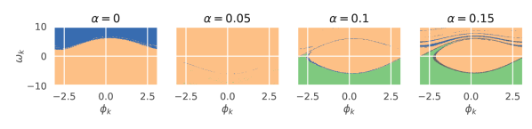
(a) Scandinavian grid

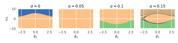
(b) Circle topology

Figure 2: Phase space cross sections. Cross section of the phase space corresponding to phase $\phi_{k}$ and phase velocity $\omega_{k}$ of a randomly chosen node of a the Scandinavian power grid and b the circle topology (both with standard parametrisation and control, see Methods). Each point belongs to the sync basin ( ), the basin of a solitary state rotating naturally ( ) or in the basin of an exotic solitary state ( ). Other asymptotic states are marked in grey ( ). Further parametrisations are given in SI.

As we will see, the physics of the power lines has a major impact on the non-linear dynamics of the power grid. In the presence of losses, the average frequency of the limit cycle is moved to $\omega_{\text{lc}}^{\prime}=\omega_{lc}-\frac{K}{D}\sin(\alpha)$. This shift dramatically alters the basin structure of the solitary, and can even flip the sign of the rotation. This leads to exotic solitary states, where an oscillator rotates in the opposite direction when coupled to the system than when uncoupled, even though the rest of the system remains in synchrony.

The dynamic effects due to losses are considerably more important than a variety of modelling assumptions that have been studied in the literature until now. They are already very pronounced for currently most studied high voltage power grids ($\alpha_{ij}\approx 0.24$, see Methods section) and become a dominant factor for future decentralized energy production with much higher losses on medium voltage power lines ($\alpha_{ij}\approx 1.4$), which are close to the theoretical stability limit of $\frac{\pi}{2}$ in the lossless case.

We begin by studying the phase space slice corresponding to the degrees of freedom of a randomly chosen node. The concrete systems we consider are the well-studied Scandinavian power grid (Fig. 1(a)) with $n=236$ nodes and a mean degree of $\bar{d}=2.7$ Menck et al. (2014); Schultz et al. (2014) as well as a regular circle topology (Fig. 1(b)) with $n=50$ nodes, a coupling radius of $R=2$ and otherwise equivalent parameter choices (see Methods section for details on the parametrization and SI for extensive meanfield analysis of this model). In the Scandinavian topology, an equal number of net producers and consumers is randomly distributed, while they are placed alternately on the circle topology.

Fig. 2 shows the result for both networks. The color indicates the asymptotic state reached after running the system with the chosen node in the plotted initial condition, and the other nodes in the synchronous state. We immediately see a dramatic change in structure for the range of $\alpha$ studied.

For a typical transmission grid as the Scandinavian one, the engineering textbooks give values of $\alpha\approx 0.24$ (see Methods section) as realistic. For both network models, even much smaller values lead to a dramatic change in the basin structure. Increasing $\alpha=0$ to $0.05$, the basin of solitary states disappears, only to reappear at $\alpha=0.15$ but mirrored as exotic solitaries, rotating contrary to the natural limit cycle. For higher values of $\alpha$, other states start playing a significant role, and the behaviour of the circle model and the Scandinavian topology start to differ.

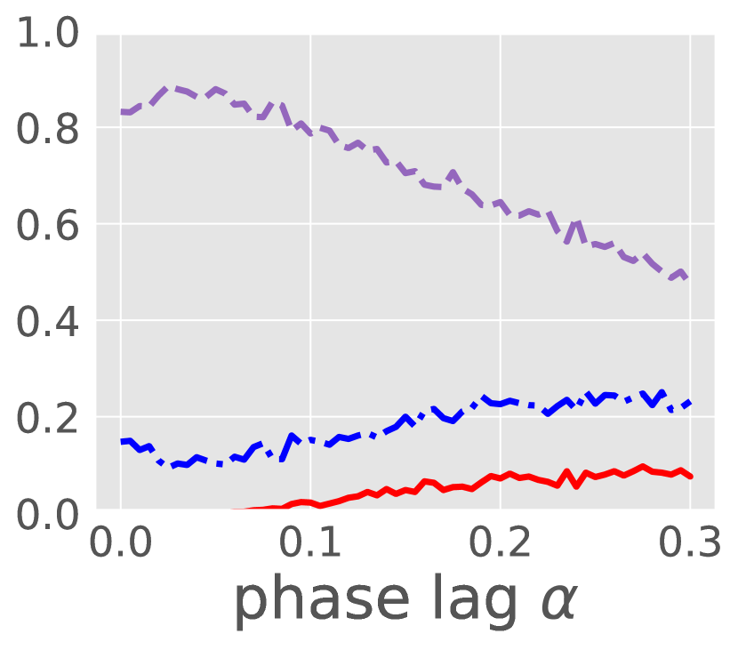
(a) ASBS - Scandinavian

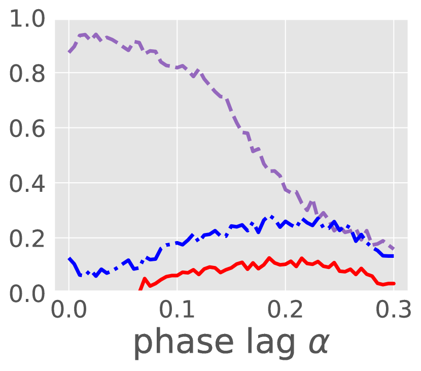
(b) ASBS - Circle

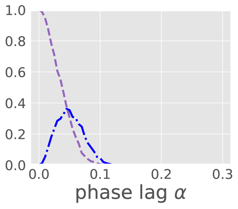
(c) global BS - Circle

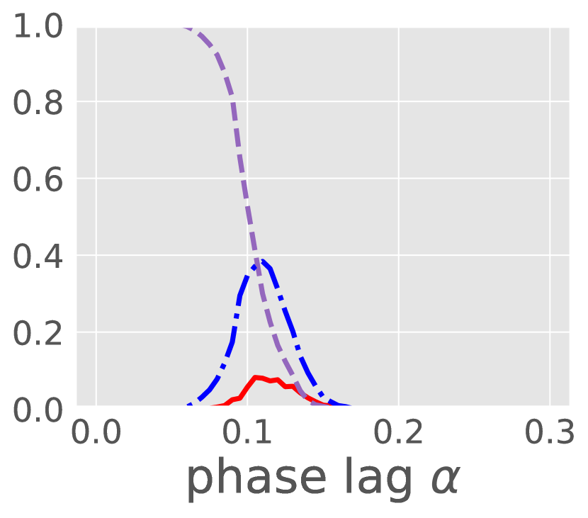
(d) high coupling

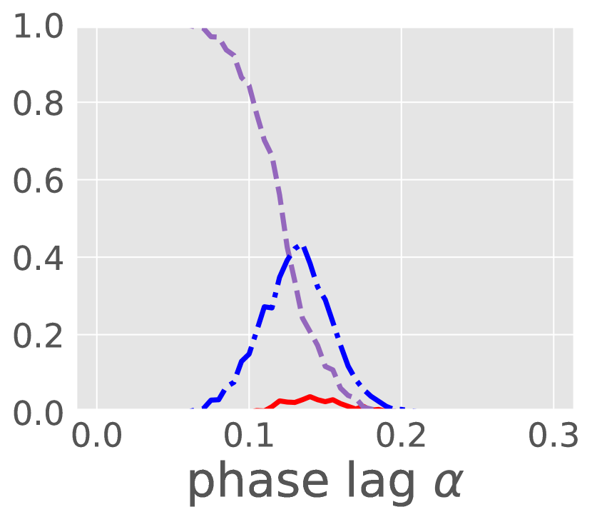
(e) medium coupling

(f) low coupling

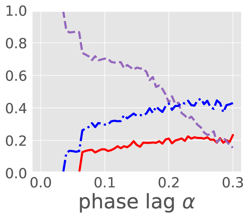
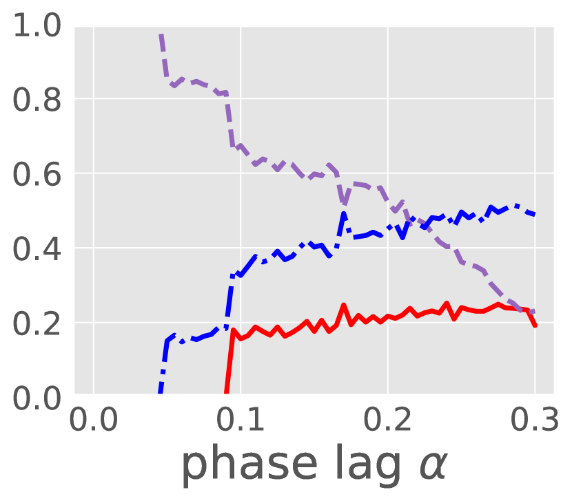
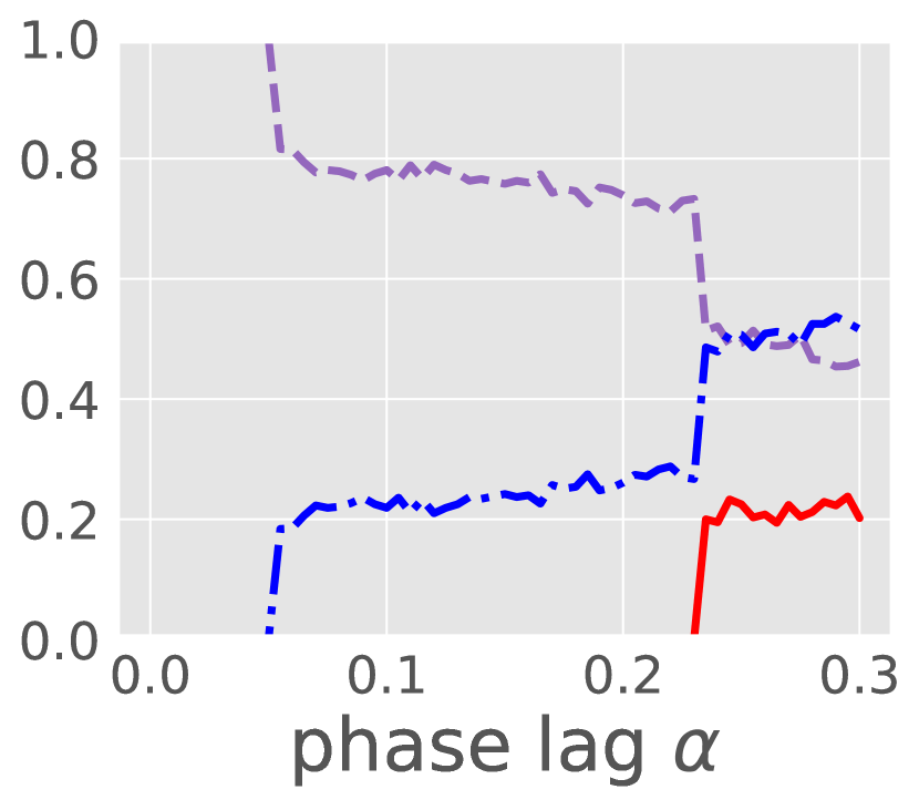
Figure 3: Basin stability. The top row shows the average single node basin stability ASBS (a, b) and the global basin stability BS (c) of three types of asymptotic regimes: synchronisation ( ), exotic solitaries ( ) and the union of normal and exotic solitaries ( ). Simulations were performed with standard parametrisation and control (see Methods). d-f global BS (top) and ASBS (bottom) for the circle topology with enhanced control and different different coupling strengths. Line styles as in a-c. Further parametrisations are given in SI.

To quantitatively study this effect, we consider the average single node basin stability (ASBS) for these systems, i.e., the probability that a perturbation at a random node will lead back to the synchronous, to a solitary, or an exotic solitary state. The ASBS of the synchronous state is a proxy for realistic large perturbations that will typically be geographically localized in the power grid, rather than perturb the system globally. We also study smaller global perturbations and likewise define a global basin stability. For a more detailed discussion of the probabilistic stability measures used here see the Methods section. Figs. 3(a) and 3(b) show that the ASBS is decreasing dramatically for both models, the Scandinavian and the circle topology, confirming the observation from the single node phase space pictures of the top two rows. In the Scandinavian power grid we see a reduction of ASBS from values larger than $0.8$ for $\alpha=0$ all the way down to $0.5$ at $\alpha=0.3$. At the same time the ASBS of solitary states is somewhat enhanced, rising from a low of $0.1$ to above $0.2$. The circle topology exhibits an even more pronounced collapse of ASBS and enhancement of the basin of solitaries, with ASBS values as low as $0.2$ for realistic values of $\alpha$. The global basin stability of the synchronous state is numerically zero in the Scandinavian topology and not shown, but for the circle topology we see a dramatic and complete collapse of stability as $\alpha$ is switched on. The stability of the synchronous state is reduced from $1$ to $0$ for unrealistically small $\alpha$ of $0.1$ already. In the intermediate regime the basin of solitaries takes over, at higher $\alpha$ we typically have several solitaries or larger clusters falling out of synchrony (see SI).

To systematically study the basin and existence of the synchronous and solitary state, we will analyse the simpler, highly symmetric circle topology further. As above, for realistic parameter choices the results are qualitatively the same for this choice of topology as for the Scandinavian power grid. In order to explore other dynamical regimes we also investigate the circle with a parametrization where the damping is much enhanced compared to the coupling and power (see Method section for details). this corresponds to an enhanced reaction of the droop control that adjusts power as a reaction to a frequency deviation. We further investigated different ratios of injected power to coupling strength, leading to differently loaded lines. In all dynamical regimes the circle topology also allows us to study the global basin stability. The detailed results are contained in the SI.

In Fig. 3 we find that the global basin stability starts at $1$ for all couplings when we have enhanced control and collapses completely when $\alpha$ is increased to realistic values. We also see that the collapse proceeds via the occurrence of a global basin of solitary states. Whereas for ASBS it is somewhat natural to expect solitary states to play a prominent role, given that only one oscillator is perturbed, here we uncover that the solitary states play a prominent role in reducing the size of the sync basin Wiley et al. (2006) in the full phase space as well.

The ASBS plots in Figs. 3(d), 3(e) and 3(f) now can be interpreted by considering the shifting of the limit cycle $\omega_{LC}^{\prime}$ with $\alpha$. While the limit cycle is not stable at $\alpha=0$, as we increase $\alpha$ its frequency gets shifted to increasingly negative values. For oscillators that are naturally rotating negatively, the limit cycle gets shifted into the parameter regime where it becomes stable first. At higher $\alpha$ the oscillators that are naturally rotating positively also gain a stable negatively rotating limit cycle, i.e. the exotic solitary described above. Note that the onset of exotic solitaries occurs at decreasing $\alpha$, i.e. for smaller losses, although the coupling strength is increased. The occurrence of other solitaries, however, is less sensitive to the coupling.

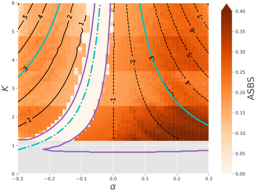
(a) Consumer, standard parametrization

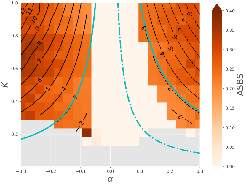
(b) Producer, enhanced control (P=0.1)

Figure 4: Existence regions. $K$-$\alpha$ parameter plane for solitary oscillations in the circle topology at a a consumer (standard parametrization) and b a producer (enhanced control). The colour scale indicates the average single node basin stability ASBS of normal respectively exotic solitaries. The contour lines give the mean instantaneous frequency of the observed solitaries as an integer multiple of the natural limit cycle $\omega_{\text{LC}}$, positive for solid, negative for dashed line style. The cyan solid lines ( ) show the analytic location of the $|\omega_{\text{LC}}^{\prime}|=3|\omega_{\text{LC}}|$ limit cycle from the infinite bus model. As a special case, the dash-dotted cyan line ( ) marks the respective hypothetical location of the $\omega_{\text{LC}}^{\prime}=0$ limit cycle. a Additionally, the purple lines ( ) mark the extend of the solitary existence regions determined by numerical state continuation (see Methods). Complementary plots for producers/consumers are given in SI.

In order to confirm this interpretation we show in Fig. 4 a systematic study of the ASBS in the $K$-$\alpha$ parameter plane, both for the standard parametrization and for the enhanced control. Note that data points below the line $K\approx P$ are excluded, since ASBS is not defined in the absence of the synchronous fixed point (see Method section for details of the numerical procedure). For comparison, we also show various markers of the infinite bus model (Eqn. 3) with shifted limit cycle $\omega_{LC}^{\prime}$. We find that the frequency of the solitary is indeed explained by the shifted frequency of the infinite bus model. Additionally, the disappearance of the solitary and the later appearance of the exotic solitary state can be understood as $\omega_{LC}^{\prime}$ being shifted close to zero, and then beyond. This suggests that both transitions from synchronisation to solitary oscillations are homoclinic bifurcations, which occur for the infinite bus model. Numerically, this is supported by a logarithmic scaling of the solitary’s oscillation period and the mean-field approximation (see SI and the discussion in Jaros et al. (2018)).

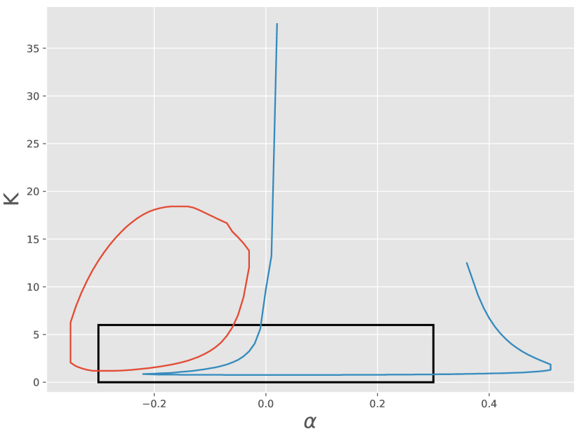
(a) Numerical continuation

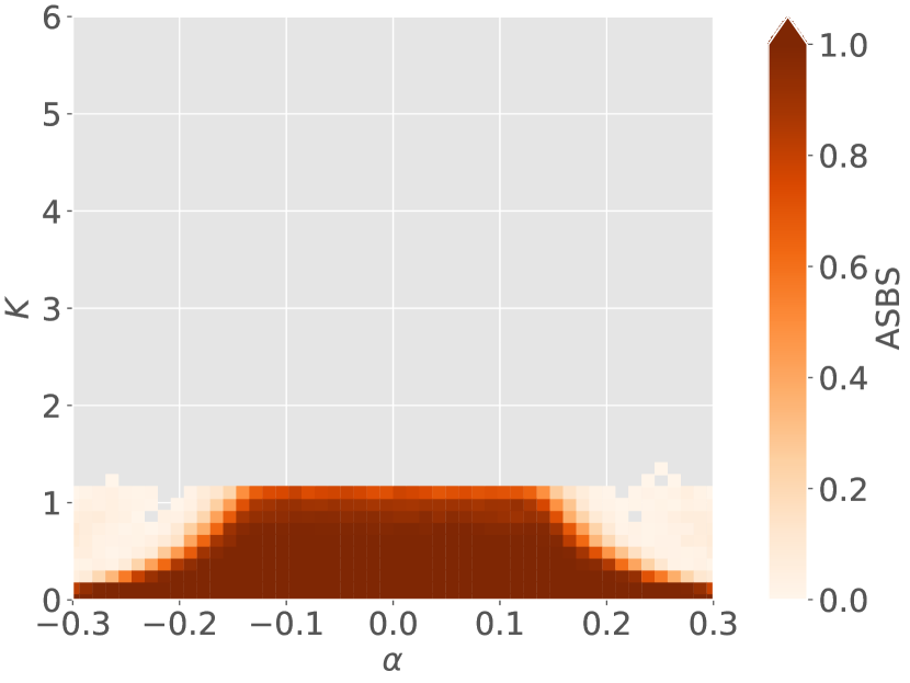
(b) global BS bimodal

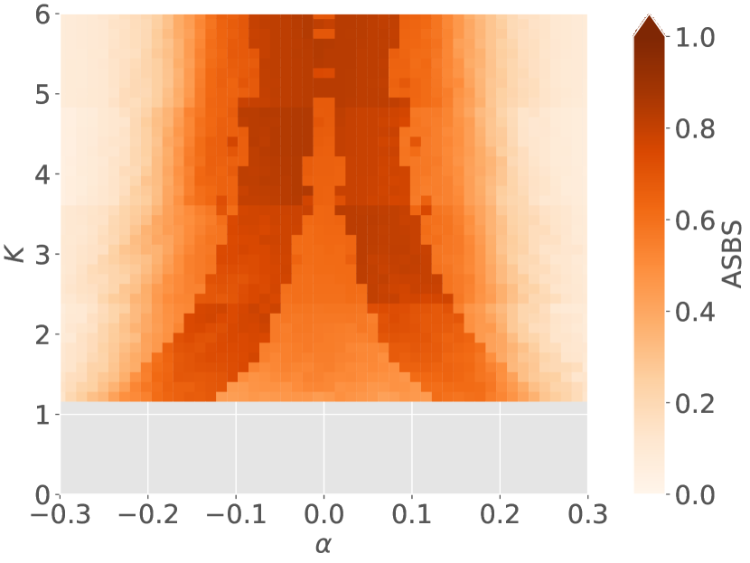
(c) ASBS synchronisation

Figure 9: Existence regions. Simulation of the circle model $R=2$ with standard parametrization and control. a Boundary of the solitary existence region from Fig. 7 with a box indicating the extent of our numerical study in b/c as well as Figs. 4 and 10. b Global basin stability estimate for the bimodal state. c Average single node basin stability estimate for the synchronous regime.

Thus for all coupling strengths in the realistic regime, there is a strong qualitative difference in the asymptotic structure between the lossless case $\alpha=0$ and realistic values for $\alpha$. Further, while the bimodal state, where all nodes oscillate close to their natural frequency $\omega_{lc}$, exists only for moderately small coupling (see SI, Fig. 9), solitary states persist even for coupling strengths much beyond realistic values. In fact, the numerical continuation of solitary states in the parameter plane suggests that, while the existence region for exotic solitaries is bounded by a maximum coupling strength, this is not the case for normal solitaries. Due to the shape of the region of existence of solitary states, an increase in coupling can even lead to exotic solitaries coming into existence.

Finally, note that, next to the single solitary states studied in the bifurcation diagram of Fig. 4, many other asymptotic states, including ones with larger desynchronized clusters and several disjoint solitaries exist. These start to play a role for larger $\alpha$ as in Fig. 2(b) (see also Jaros et al. (2018), SI).

In summary, for all studied parameter regimes – including the case of a realistically parametrized Scandinavian system – we observe a dramatic reduction of the size of the basin of attraction of the synchronous desirable operating state when going to realistic values of losses. To our knowledge, this very generic phenomenon has not been observed in the literature before. It has far reaching implications for the design and control of future power systems. Our results show that it is not possible to use theoretical results on the stability of systems without losses ($\alpha=0$) in the design of future power systems as is. The losses fundamentally alter the dynamical behaviour of the coupled systems.

While we find that an enhanced control effort is not sufficient to suppress solitary states, a strong control regime, with an extremely high ratio $\frac{D^{2}}{PH}$ of a hundred times that of the standard value (see Methods), can stabilize the system up until $\alpha\lessapprox 0.2$ (see SI, Fig. 11(f)). Beyond this, however, for realistic values of $\alpha\approx 0.24$ the global stability is already rapidly collapsing while ASBS is slowly decreasing. For future distribution grids with $\alpha$ much larger than $0.24$ even such a probably unrealistic, and for other reasons undesirable, control effort is not sufficient to eliminate the multistability induced by the losses.

Further, as noted above, a mere increase of coupling, e.g. by improving transmission capacities in a power grid, does not suffice to prohibit non-synchronous solitary oscillations either. In some specific situations it can even enhance their basin. Controling such lossy dynamical networks and solitaries in them thus poses a fundamental challenge, to future research in network control that can not be answered by tweaks to system parameters.

The study of lossy coupling also has implications for the engineering literature. While case studies typically work with the physically correct equations involving losses (e.g. Liu and Zhang (2017)) it is also typical to neglect the losses of e.g. coupled two-area systems Ulbig et al. (2014). It remains unclear whether this is justified. Novel control strategies based on basin structure of the lossless case, like those in Vu et al. (2017), will certainly need to be revisited. The degree to which the presence of losses also affects the transient and stochastic behaviour of the power grid is also a subject of ongoing research Auer et al. (2017).

The fact that this effect appears to be not strongly affected by the network topology means that further investigations – including experiments and analytics – can begin on simplified systems, and the effect can be cleanly isolated from pronounced local topological effects present in real world topologies. In particular, solitary states persist even in the mean-field limit with an all-to-all coupling, as we extensively discuss in the SI.

Finally, as noted before, the model studied here can be equivalently seen as representing generic Newtonian oscillators, coupled by the lowest Fourier mode. When approximating general systems as phase oscillators (see e.g. Nakao (6 04)), the parameter $\alpha$ appears generically. We therefore expect the phenomenon described here to pertain to a wide range of non-linear heterogeneous oscillator systems.

Methods

Parametrization of networks and dynamical regimes.

Typical values for ohmic losses and inductivity in power grids areAuer et al. (2016):

Line	Transmission	Distribution	Low voltage
R $[\Omega/km]$	0.1	0.4	0.5
X $[\Omega/km]$	0.4	0.3	0.08
$\alpha$	0.24	0.93	1.41

Thus the regime studied in this work covers transmission lines, where the lossless approximation has been taken to be valid.

The power grid is then parametrized in accordance with the values most studied in the basin stability literature Menck et al. (2014); Nitzbon et al. (2017); Schultz et al. (2014), $H=1$, $P=1$, $D=0.1$, and $K\approx 6$ for the geographic power grid, and $K=6$ for the circle topology.

This parametrisation is typically used in the theoretical physics literature in order to study network and multistability effects expected to be relevant in future power grids. It is not expected to be a very close representation of current power grids, but to reveal structural features of the type of dynamics expected in future power grids. As the observed phenomenon is highly generic, and depends primarily on the physics of the coupling, we expect it to occur in all parametrizations of the swing equation though.

In order to be self-contained we will briefly review the detailed motivation behind the parametrisation used. Currently each node in a transmission grid connects large-scale conventional power plants or serves as the connection point of underlying distribution grids. In the future, increasingly decentral power generation in active distribution grids, means that every transmission node effectively represents a region with a net power output that can be either positive or negative. Assuming that the location and production of decentral generation is not correlated with the existing grid structure, it is reasonable to simply choose at random whether a region is producing or consuming.

In the classical case, consumer regions are modelled as constant demands and the dynamics occurs purely at the generators. As a reduction of conventional generation reduces system inertia, we expect grid-forming inverter-interfaced distributed generation units to contribute to overall system inertia as well as droop control. Thus load nodes are reasonably modelled by inertial, damped nodes with a net power demand.

We believe that a random assignment of net generation/consumption without pre-assuming the actual amount is a plausible first-order model for the described scenario.

Dynamical regimes.

The bifurcation structure of the system is time parametrization invariant, and thus there are two characteristic quantities in the system. Meaningful choices for time invariant parameter combinations are $\frac{P}{K}$, which characterizes the load on the lines, and $\frac{D^{2}}{PH}$ which describes the strength of the droop control relative to the power infeed.

Next to the standard parametrization, we also studied a strongly damped regime with enhanced droop control driving the system to the fixed point, and an extremely strong droop control, for which the results are shown in the SI, Fig. 11(f).

	Standard	Enhanced control	Strong control
$\frac{D^{2}}{PH}$	$1/100$	$1/10$	$1$

We further varied the coupling strength, and hence the line loading.

	Standard	High	Medium	Low coupling
$\frac{P}{K}$	$\approx 1/6$	$1/20$	$1/10$	$1/2.5$

Probabilistic stability anlysis.

The main numerical method we apply here is the sampling-based evaluation of probabilistic properties of dynamical systems Hellmann et al. (2016); Lindner and Hellmann (2018); Menck et al. (2014, 2013); Nitzbon et al. (2017); Schultz et al. (2018, 2017). In particular, basin stability is the probability that a system converges to a specific attractor given a distribution of random perturbations. This can be regarded as a volume measure of the attraction basin. In the context of synchronisation it became popular as the ’size of the sync basin’ Wiley et al. (2006). A direct evaluation of the basin geometry is computationally not feasible in high-dimensional systems. Even if the set is known to be convex, current algorithms scale with $\mathcal{O}(n^{4})$ where $n$ is the phase space dimension Lovasz and Vempala (2003). Instead, a Monte Carlo sampling yields efficient estimates of the volume, whose standard error does not depend on $n$ Menck et al. (2013).

Compared with mathematical methods based on Lyapunov functions, the advantage and draw back of sampling based methods is that they are not sensitive to worst case scenarios. Instead, they provide accurate results on the typical behaviour of a dynamical system, even where analytic results are hard to achieve or not available.

The perturbations are drawn uniformly at random from a finite box centered around the synchronous state. The synchronous state itself changes with $\alpha$ and thus the box of initial conditions does, too. Fig. 5 in the SI illustrates how the synchronous state changes with alpha.

We use both global perturbations, where the perturbations apply to the all phase space variables, and network-local perturbations where perturbations are localized at a particular node. Unless otherwise specified, global basin stability was obtained by sampling from initial conditions with $\Delta\dot{\phi}_{i}\in[-0.1\omega_{lc},+0.1\omega_{lc}]$ and $\Delta\phi_{i}\in[-\pi,+\pi]$. Our second measure is the average single node basin stability, the probability to run to a particular state after a perturbation at a randomly drawn node, drawn from $\Delta\dot{\phi}_{i}\in[-1.5\omega_{lc},+1.5\omega_{lc}]$ and $\Delta\phi_{i}\in[\phi_{i}^{\ast}-\pi,\phi_{i}^{\ast}+\pi]$. Here, the $\phi_{i}^{\ast}$ denote the phase values at the synchronous fixed point, i.e. ASBS is determined by perturbing a randomly chosen node’s degrees of freedom away from the fixed point. This particular choice of perturbations is the key difference to the determination of global basin stability. Consequently, ASBS cannot be determined in the absence of a synchronous regime for certain parameter values.

For the standard configuration the global basin stability is numerically not distinguishable from zero. One way to interprete this is that each oscillator has a finite probability to desynchronize and perturbing all at the same time makes the probability that none of them do exponentially small. The average single node basin stability is a more robust and more realistic measure of the stability of the synchronous state.

Continuation Study

To perform a numerical continuation of solitary states in the parameter plane (see Fig. 4(a)), we integrated the system with a Cash–Karp method (error $e=10^{-4}$) for $T=5\cdot 10^{3}s$ under the influence of small noise (amplitude $d=10^{-5}$) to ensure transverse stability. $T$ is chosen large enough to exclude transient solitary desynchronisation. From a starting point, one of the parameters is varied in steps of $\Delta\alpha=0.01$ respectively $\Delta K=0.1$ until the solitary oscillation ceased to exist. Then, the last step is reversed and the algorithm adds one step to the other parameter, tracking a bifurcation line.

Software

Simulations were performed using the Scipy package Jones et al. (2001) and the pyBAOBAP package available at https://gitlab.pik-potsdam.de/hellmann/pyBAOBAP. Scipy uses the LSODA solver of the odepack Library Hindmarsh (1983).

All code and data will be published open source at https://gitlab.pik-potsdam.de/pschultz/solitary_power_grid or is available upon request.

Supplemental Information (SI)

Derivation of the Power Flow Equation

Here, we derive the lossy power flow equation (Eqn. 2). $P_{ij}$ should be the outgoing flow at the node such that the power flow equation reads $P_{i}=\sum_{j}P_{ij}$. According to Ohm’s law, the current on a line is given by $\frac{V_{i}-V_{j}}{R_{ij}+iX_{ij}}$, (if the own voltage is higher, current, and hence energy flows away) or $Y_{ij}(V_{i}-V_{j})$. As $R_{ij}$ and $X_{ij}$ are positive, $Y_{ij}$ has positive real part and negative imaginary part. The Laplacian $L_{ij}=\delta_{ij}\sum_{k}Y_{ik}-Y_{ij}$ then provides us with the total outgoing current: $I=L\cdot V$. To connect with the literature written in terms of phase lags $\alpha$, we set $Y=-iKe^{i\alpha}$. Then $Ke^{i\alpha}=iY$ has a positive real part and a positive imaginary part. Hence $K$ and $\alpha$ are positive.

Using $V_{i}=e^{i\phi_{i}}$, $V_{i}V_{i}^{\star}=1$, the power flow can then be written as follows:

$$\sum_{j}P_{ij} =\Re(V_{i}I_{i}^{\star})$$

$$=\Re\left(\sum_{j}V_{i}L_{ij}^{\star}V_{j}^{\star}\right)$$

$$=\Re\left(V_{i}V_{i}^{\star}\sum_{k}(-ie^{-i\alpha_{ik}}K_{ik})^{\star}\right)-\Re\left(\sum_{j}V_{i}(-ie^{-i\alpha_{ij}}K_{ij})^{\star}V_{j}^{\star}\right)$$

$$=\Re\left(iV_{i}V_{i}^{\star}\sum_{k}e^{-i\alpha_{ik}}K_{ik}\right)-\Re\left(i\sum_{j}V_{i}e^{-i\alpha_{ij}}K_{ij}V_{j}^{\star}\right)$$

$$=-\Im\left(\sum_{k}K_{ik}e^{-i\alpha_{ik}}\right)+\Im\left(\sum_{j}K_{ij}e^{i(\phi_{i}-\phi_{j}-\alpha_{ij})}\right)$$

$$=-\sum_{k}K_{ik}\sin(-\alpha_{ik})+\sum_{j}K_{ij}\sin(\phi_{i}-\phi_{j}-\alpha_{ij})$$

$$=\sum_{j}K_{ij}\left(-\sin(-\alpha_{ij})+\sin(\phi_{i}-\phi_{j}-\alpha_{ij})\right)$$

Synchronous Regime with Varying Losses

In Fig. 5 we depict the shift of the synchronous operating point under an increase of losses which appear as a phase shift $\alpha$ in Eqn. 1. The simulation was performed for the Scandinavian power grid with standard parametrization and enhanced control.

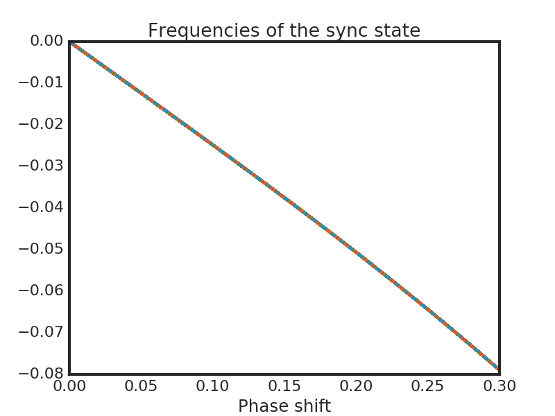
(a) Instantaneous frequency

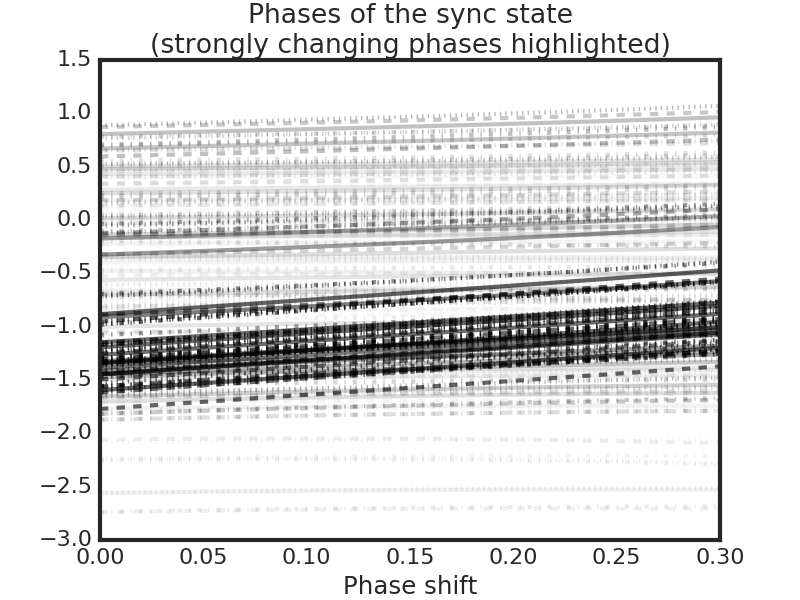
(b) Phases

Figure 5: Synchronous regime. Variation of the synchronous frequency (a) and phases (b) with increasing phase shift $\alpha$.

Circle Model of the Power Grid

In this section we consider an abstract power grid organization, the so-called circle model, which demonstrates the main features we find responsible for prompt desynchronization. In this model, the desired synchronized state exists and is stable. However, the model itself appears to be genuinely multistable. There arise indeed many other, so-called solitary states in which one or a few power grid units start to behave differently with respect to all others perfectly synchronized such that not only the phase but also the average frequency deviates from the synchronous behaviour. Remarkably, these solitary states are Lyapunov stable too and hence, they cannot be excluded from the global system dynamics even by an essential increase of the inner network connectivity (as it would be naturally expected). Furthermore, it is found that this kind of network multistability arises under realistic operating parameters applied to power grids. If so, there is always a danger that sudden non-small disturbances associated e.g. with fluctuations in production or demand may trigger desynchronization of one or several power generators/consumers even if the synchronous state is perfectly operating in a stable regime. While our model is topologically simplified and does not account for complication of the real power grid structure, we show through extensive numerical experiments that our predictions remain robust when including these effects for the Scandinavian power grid.

Define the circle power grid as follows. Let it contains $N$ units and let a half of them, $N/2$, be identical generators (representing power plants) and the other half identical motors (representing consumers). Place all of them on a ring with the ”alternative” disposition, Fig. 1(b), and assume that each unit is connected with $R$ of its nearest neighbours to the left and to the right, and with an equal coupling strength $K$. In the case, all units obey the same type of equation of motion, the Kuramoto model with inertia, of the form

$$\ddot{\phi}_{i}+\epsilon\dot{\phi}_{i} =(-1)^{i+1}\Omega+2RK\sin\alpha+K\sum\limits_{j=i-R,j\neq{i}}^{i+R}\sin(\phi_{j}-\phi_{i}+\alpha)\;$$ (5)

($i=1,\dots,N$), where the term $K\sin\alpha$ in the right-hand side arises due to assigned self-coupling topology of the model connectivity. It shifts the oscillator eigenfrequency $\Omega$ up or down depending on the sign of the parameter $\alpha$.

Here, we use the notation

$$\begin{split}\Omega&:=|P_{i}|/H,\;\;\forall\;i\\ \epsilon&:=D_{i}/H,\;\;\forall\;i\\ K&:=K_{ij}/H,\;\;\forall\;i,j\;.\end{split}$$ (6)

In the lossless case $\alpha=0$ this term disappears and one comes to the classical Kuramoto model with bi-modal frequency distribution

$$\ddot{\phi}_{i}+\epsilon\dot{\phi}_{i} =(-1)^{i+1}\Omega+K\sum\limits_{j=i-R}^{i+R}\sin(\phi_{j}-\phi_{i})\;$$ (7)

which dynamics is comparably simpler. Introducing non-zero $\alpha$, however, makes the global network behaviour more involved due to multiple appearance of solitary states, not avoidable even with large increase of the coupling strength $K$.

Synchronous State of the Circle Model

To identify a synchronous state of the circle power grid model (Eqn. 5), re-write it in a two-group form denoting the generators by $\theta_{i}$ and the consumers $\psi_{i},~{}i=1,\dots,N/2$:

$$\ddot{\theta}_{i}+\epsilon\dot{\theta}_{i} =+\Omega+2RK\sin\alpha+K\sum\limits_{j=i-R,j\neq{i}}^{i+R}\sin(\theta_{j}-\theta_{i}+\alpha),$$

$$\ddot{\psi}_{i}+\epsilon\dot{\psi}_{i} =-\Omega+2RK\sin\alpha+K\sum\limits_{j=i-R,j\neq{i}}^{i+R}\sin(\psi_{j}-\psi_{i}+\alpha).$$ (8)

Assume $\theta_{1}=\dots=\theta_{N/2}\equiv\theta$ and $\psi_{1}=\dots=\psi_{N/2}\equiv\psi$, and subtract the second equation from the first one. The following equation is obtained for the phase difference $\eta=\theta-\psi$:

$$\ddot{\eta}+\epsilon\dot{\eta}=2\Omega-RK(\sin(\eta+\alpha)+\sin(\eta-\alpha)),$$ (9)

By simple trigonometry, it can be re-written as

$$\ddot{\eta}+\epsilon\dot{\eta}=2\Omega-\mu\cos\alpha\sin\eta,$$ (10)

where a new coupling parameter $\mu=2RK$ is introduced. This is an equation of motion in the two-dimensional invariant manifold indicated by the conditions $\theta_{1}=\dots=\theta_{N/2}\equiv\theta$, $\psi_{1}=\dots=\psi_{N/2}\equiv\psi$ as above. Synchronous states of the original $N$-dim Eqn. 5 are given by the roots of its right-hand side, which are

$$\eta_{O}=\arcsin\frac{2\Omega}{\mu\cos\alpha},~{}~{}~{}~{}\eta_{S}=\pi-\arcsin\frac{2\Omega}{\mu\cos\alpha}$$ (11)

corresponding to stable node $O=(\eta_{O};0)$ and saddle $S=(\eta_{S};0)$ of the in-manifold scalar Eqn. 10. The states are born in a saddle-node bifurcation at the bifurcation curve

$$\mu_{sync}=\frac{2\Omega}{\cos\alpha},$$ (12)

and they exist for all $\mu>\mu_{sync}$, where node $O$ transforms into a stable focus soon after the bifurcation at $\mu_{foc}=\frac{2\Omega}{\cos\alpha}\sqrt{1+\epsilon^{4}/64}$.

The synchronous state we are looking for is given by the stable equilibrium $O$. The in-manifold stability, however, does not guarantee its transverse stability. Our numerics indicate, however, that the equilibrium $O$ is also stable in the whole $N$-dimensional space of the original model Eqn. 5.

We conclude that the synchronous state of the circle model (Eqn. 5) is born in a saddle-node bifurcation as the coupling strength $\mu$ exceeds the bifurcation value $\mu_{sync}$ and it preserves the stability with further increase of $\mu$. In the state, generators and consumers create two phase-synchronized groups with the phase shift between them equal $\eta_{O}$. At the saddle-node bifurcation curve $\mu=\mu_{sync}$, the phase shift is $\eta_{O}=\pi/2$ and it decreases to zero as $\mu\rightarrow\infty$. Frequency $\Omega_{O}$ of the synchronous state $O$ is obtained from Eqn. 5 as:

$$\Omega_{O}=-\frac{\mu\sin\alpha}{2\epsilon}(1-\sqrt{1-(\frac{2\Omega}{\mu\cos\alpha})^{2}})=-\frac{\mu(1-\cos\eta_{O})}{2\epsilon}\sin\alpha.$$ (13)

It follows therefore that synchronous frequency $\Omega_{O}$ is zero in the lossless case $\alpha=0$, negative for $\alpha>0$ and positive for $\alpha<0$.

Solitary states in mean-field coupled circle model

Solitary states can be derived analytically in the case of mean-field approximation of the circle model, i.e. when $R=N/2$ in Eqn. 5. For convenience, we write the mean-field model in the standard normalized form

$$\ddot{\phi}_{i}+\epsilon\dot{\phi}_{i} =(-1)^{i+1}\Omega+\frac{\mu}{N}\sum\limits_{j=1}^{N}\sin(\phi_{j}-\phi_{i}-\alpha)\;.$$ (14)

Here parameter $\alpha$ can be positive or negative. Due to the assigned symmetry, these two cases are reducing explicitly to each other by simple transformation $\alpha\rightarrow-\alpha,~{}\Omega\rightarrow-\Omega,~{}\phi_{i}\rightarrow-\phi_{i}$, at which the generators and consumers exchange their network disposition. Therefore, the system dynamics appears to be equivalent for $\alpha<0$ and $\alpha>0$ and if so, only one of the cases should be derived. The symmetry property is also valid for the general, non mean-field form of the circle power grid model (Eqn. 5), which is clearly demonstrated by our simulations. However, it is not the case for non-symmetric generator/consumer disposition as it is normally the case in real power grid networks, e.g. in the Scandinavian power grid.

The synchronous state $O$ of the mean field-model Eqn. 14 is obtained by the same procedure as in the previous section applied to the two-group representation Eqn. 8 including generators $\theta_{i}$ and consumers $\psi_{i}$:

$$\ddot{\theta}_{i}+\epsilon\dot{\theta}_{i} =+\Omega+\frac{\mu}{N}\sum\limits_{j=1}^{N/2}(\sin(\theta_{j}-\theta_{i}-\alpha)+\sin(\psi_{j}-\theta_{i}-\alpha)),$$

$$\ddot{\psi}_{i}+\epsilon\dot{\psi}_{i} =-\Omega+\frac{\mu}{N}\sum\limits_{j=1}^{N/2}(\sin(\psi_{j}-\psi_{i}-\alpha)+\sin(\theta_{j}-\psi_{i}-\alpha)).$$

So, it has the form

$$O:~{}\theta_{1}=\dots=\theta_{N/2}\equiv\theta,~{}~{}\psi_{1}=\dots=\psi_{N/2}\equiv\psi$$ (16)

with a constant phase shift $\eta_{O}=\theta-\psi$ between generators and consumers, where $\eta_{O}=\arcsin\frac{2\Omega}{\mu\cos\alpha}$; exists and is stable for all $\mu$ above the bifurcation curve as in 12.

Beyond the the existence of synchronous state $O$ which is phase and frequency synchronized, numerous solitary states of different configurations are typically arising in the mean-field model (Eqn. 14). They consist normally of several phase clusters, each rotating with its own frequency, manifesting in such a way a phenomenon of frequency clustering. This peculiar phenomenon differs from usual phase clustering well-known in (pure) phase oscillatory networks, cr. standard Kuramoto model. De facto, due to the presence of inertia, the system dynamics becomes much more involved. The main peculiarity is an enormous multistability, i.e., when the number of co-existing stable solitary and other states can grow exponentially with the system size $N$, moreover, in an essential domain of the system parameters. If so, spatial chaos Elphick et al. (1987); NIZHNIK et al. (2002); Omelchenko et al. (2011) becomes an inherent characteristic of the model. We are coming apparently to a new reality, still not comprehended, in the field of coupled oscillators with inertia.

The simplest but not trivial solitary-type behaviour is supplied by a 1-solitary state, where just one generator or consumer- let for definiteness it be a generator $\theta_{1}$ - splits off from the others, which are frequency synchronized consisting of two phase clusters: one of remaining generators and the other of all consumers, i.e.,

$$\Phi_{1-sol}:~{}\theta_{1}\equiv\gamma;~{}\theta_{2}=\dots=\theta_{N/2}\equiv\theta,~{}\psi_{1}=\dots=\psi_{N/2}\equiv\psi.$$ (17)

Examples of four different 1-solitary states for the mean-field model (Eqn. 14) are illustrated in Figure 6, for solitary generator (b,c) and consumer (a,d). Due to the model symmetry, the case with solitary consumers can be reduced to the generator one by simple parameter/variable change $\alpha\rightarrow-\alpha,~{}\Omega\rightarrow-\Omega,~{}\phi_{i}\rightarrow-\phi_{i}$. We skip it in the section and concentrate further on the states with a solitary generator as in Fig. 6.

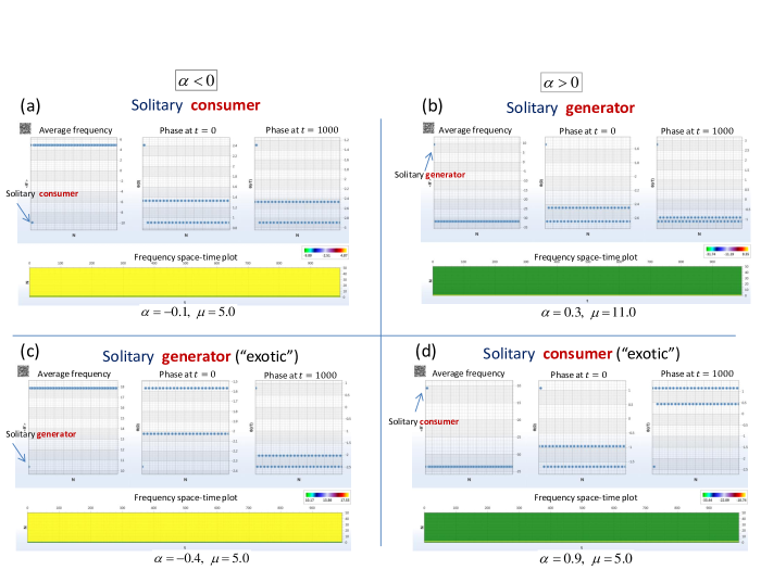
Figure 6: (colour online). 1-solitary states in mean-field coupled model (Eqn. 14). Mean frequency, and two phase snapshots are shown above, and frequency space-time plot is below. All simulation starting from random initial conditions, the behaviour is shown after transient $T=10^{4}$ time units. Parameters as in the main text.

As it is illustrated in Fig. 6, there are two types of 1-solitary states in which a generator is detached. Actually, what is happened in both cases, the generator continues to rotate close to its eigenfrequency $\Omega=10$ in the situation when all others units synchronize with smaller (b) or larger (c) mean frequency. The first situation (b) is maybe considered a ”normal”, as the desirable synchronous frequency should naturally be less then those of the generators, and it equals zero if $\alpha=0$ and deviates to negative values as $\alpha>0$. Another 1-solitary state shown in (c) obeys a counter-intuitive property: the mean frequency of the synchronous cluster appears to be larger then 10, we call this state an ”exotic”, and it exist for negative $\alpha$ only.

The parameter region for both, ”normal” and ”exotic” 1-solitary states (with a generator detached) are shown in Fig. 7. Analogous regions for the case with a consumer detached (see examples in Fig. 6 (a,d)) are symmetrically disposed with respect to the $\alpha=0$ axis.

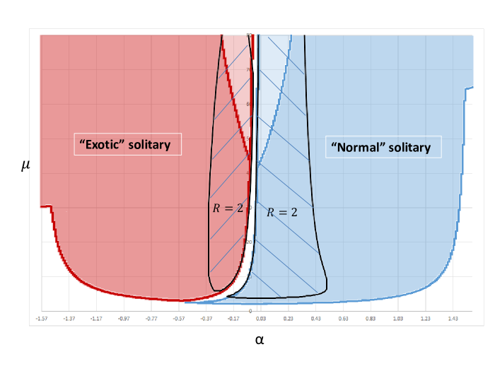
Figure 7: (colour online). Parameter regions for both, “normal” and “exotic” 1-solitary states in the mean-field coupled model Eqn. 14 (coloured) and the respective locally coupled model with coupling radius $R=2$ (dashed). Parameters as in the main text.

Reduction to Solitary Manifold

In the new variables $(\gamma,\theta,\psi)$ for 1-solitary state (Eqn. 17) the mean-field model (Eqn. 14) consists of only three equations:

$$\ddot{\gamma}+\epsilon\dot{\gamma} =+\Omega+\frac{\mu}{N}((\frac{N}{2}-1)\sin(\theta-\gamma-\alpha)+\frac{N}{2}\sin(\psi-\gamma-\alpha)+\sin(-\alpha)),$$

$$\ddot{\theta}+\epsilon\dot{\theta} =+\Omega+\frac{\mu}{N}(\frac{N}{2}\sin(\psi-\theta-\alpha)+\sin(\gamma-\theta-\alpha)+(\frac{N}{2}-1)\sin(-\alpha)),$$

$$\ddot{\psi}_{i}+\epsilon\dot{\psi}_{i} =-\Omega+\frac{\mu}{N}((\frac{N}{2}-1)\sin(\theta-\psi-\alpha)+\sin(\gamma-\psi-\alpha)+\frac{N}{2}\sin(-\alpha)).$$

This is a reduced model of three coupled virtual ”pendula” governing the dynamics in the respective 6-Dim solitary manifold. The pendula are linear but the coupling terms, however, are strongly non-linear (contain sinusoidal functions). This results in complex dynamical behaviour characterized by multiple solitary states and chaos. As coupling terms depend only on the phase differences, the system dimension can be further reduced by introducing phase difference variables $\nu=\gamma-\psi,~{}~{}\eta=\theta-\psi$. In the new variables, only two equations are left:

$$\ddot{\nu}+\epsilon\dot{\nu} =2\Omega+\frac{\mu}{2}((1-\frac{2}{N})\sin\alpha-\sin(\nu+\alpha)+\frac{2}{N}\sin(\nu-\alpha)+(1-\frac{2}{N})(\sin(\eta-\nu-\alpha)-\sin(\eta-\alpha))),$$

$$\ddot{\eta}+\epsilon\dot{\eta} =2\Omega+\frac{\mu}{N}\sin\alpha-\frac{\mu}{2}(\sin(\eta+\alpha)+(1-\frac{2}{N})\sin(\eta-\alpha))+\frac{\mu}{N}(\sin(\nu-\eta-\alpha)-\sin(\nu-\alpha)).$$

This is a system of only two coupled ”pendula”, maintaining on a 4-Dim invariant manifold of the whole $N$-dimensional phase space. It is complicated for analytic study, as each pendulum as well as all coupling terms are non-linear. However, the model is low-dimensional so it can be easily derived in a standard way with use of numerical simulations to identify 1-solitary states for the $N$-dimensional mean-field model (Eqn. 14), up to the thermodynamic limit $N\rightarrow\infty$. Note, that all in-manifold regimes which develop within the framework of the reduced system (Eqn. LABEL:1-sol_system-4) should be tested on the transverse stability with respect of out-of-manifold perturbations, to guarantee the existence in the whole $N$-dimensional model.

This approach is also applicable to $k$-solitary states, with any $k=2,3..$, of the form

$$\Phi_{k-sol}:~{}\theta_{1}=\dots=\theta_{k}\equiv\gamma;~{}\theta_{k+1}=\dots=\theta_{N/2}\equiv\theta,~{}\psi_{1}=\dots=\psi_{N/2}\equiv\psi.$$ (20)

Reduced low-dimensional systems for the $k$-solitary states can be obtained in a similar way as in the $k=1$ case above. They are slightly different with the system parameters however, their dimensions are the same. Note finally, that the behaviour of solitary states becomes even more puzzled if the synchronized elements, variables $\theta_{i}$ and $\psi_{i}$ in (Eqn. 20), split off by more then two clusters. Above reduced procedure still works, however, the dimension of the ”solitary” manifold becomes larger then $4$. Nevertheless, the study in this case is yet much simpler then the original $N$-dimensional model.

Homoclinic Bifurcation of Solitary Oscillations

As can be seen for instance in Fig. 4, solitary oscillations cease to exist beyond a critical value for the losses $\alpha$ (at fixed coupling strength). Our numerical studies give a strong indication that the underlying mechanism is a homoclinic bifurcation of the solitary limit cycle towards synchronisation. Furthermore, this is also suggested by our analogy with the infinite-bus-model. The numerical procedure is as follows: The period of the solitary oscillation is estimated as the inverse time average of the phase velocity $\omega_{s}$ at the solitary node with index $s$:

$$\tau=\frac{2\pi}{\overline{\omega_{s}}}=2\pi T\left(\int\limits_{0}^{T}~{}dt\;\omega_{s}(t)\right)^{-1}$$ (21)

for some large enough $T$ such that we can be sure to measure several periods. Varying the phase lag $\alpha$ as the control parameter, we used the period $\tau$ estimated at one parameter value to set $T=10\tau$ for the next (updated) parameter value. The numerical integration is performed using SciPy’s CVode solver with step size $10^{-3}$.

In case of a homoclinic bifurcation, it is expected that the period $\tau$ scales logarithmically with the parameter in proximity to the bifurcation point $\alpha_{c}$, i.e. $\tau\simeq\log|\alpha_{c}-\alpha|$ (see for instance Strogatz (2018)).

]

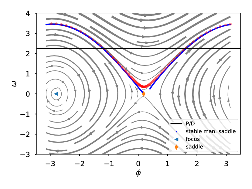
(a)

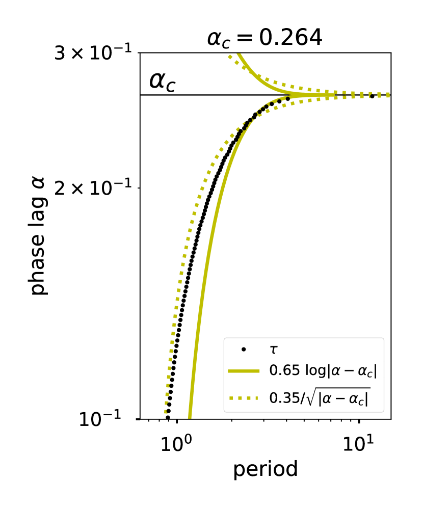
(b)

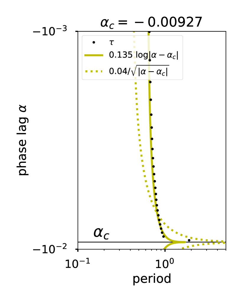
(c)

Figure 8: Bifurcation analysis. a Phase space of the infinite bus model $P=1$, $D=0.1$, $K=2$, $H=1$. The positions of the stable focus, the saddle and its stable manifold are indicated. The horizontal black line indicates the value of $\omega_{lc}^{\prime}$. See the text for further discussion. b Bifurcation analysis of the infinite bus model with above parameters. c Bifurcation analysis of the circle model with standard parameters and control. b,c The yellow lines depict logarithmic and square root scaling laws with suitable parameters as visual guidance.

Consider the phase portrait of the infinite bus model ($P=1$, $D=0.1$, $K=2$, $H=1$) close to the bifurcation point at $\alpha_{c}\approx 0.263$ pictured in Fig. 8(a). The red circles correspond to 100 initial conditions equally spaced on the limit cycle. Firstly, the locus of the limit cycle is close to the stable manifold of the saddle point (determined by backward integration) before they merge into a homoclinic orbit at $\alpha_{c}$. Secondly, the distribution of points clusters near the saddle, indicating an increase of $\tau$ close to $\alpha_{c}$ due to a slowing down of trajectories. The numerically determined values of $\tau$ are given in Fig. 8(b). As a guidance to the eye, the solid yellow line depicts a logarithmic scaling as expected for the homoclinic bifurcation in the infinite bus model. For comparison, the dashed yellow line gives a square root scaling in the case of an infinite-period bifurcation. It appears that close to $\alpha_{c}$ the logarithmic function is a better candidate for the scaling $\tau(\alpha)$, the onset of the divergence is much steeper than expected for the square root case. Analogously, $\tau(\alpha)$ is estimated for the circle model, here for the standard parametrization and control. From Fig. 4(a) at $K=6$, one expects a bifurcation at slightly negative $\alpha_{c}\approx-0.009$ from normal solitary oscillations to synchronisation. Repeating our analysis from the infinite bus model for the circle indeed strongly suggests a homoclinic bifurcation (Fig. 8(c)). In summary, our numerical investigations and the analogy to the infinite bus approximation support the hypothesis that the global bifurcation curves in the parameter plane of the circle model are homoclinic.

Additional Parameter Plane Studies

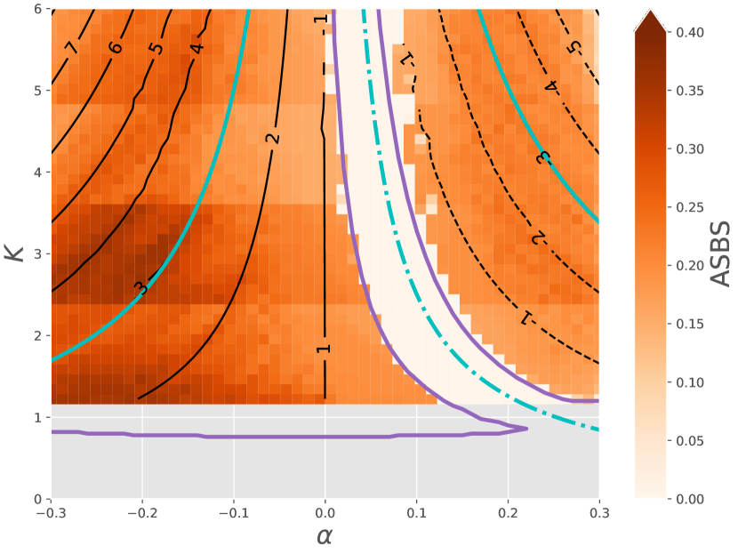
(a) Producer, standard parametrization

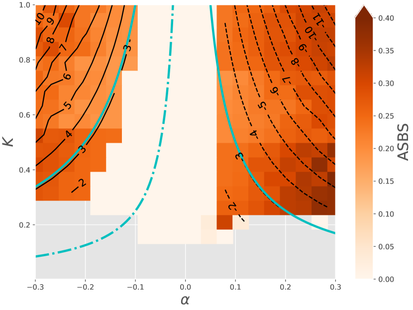
(b) Consumer, enhanced control

Figure 10: Existence regions. a,b As Fig. 4, with producer/conusmer exchanged.

Additional Basin Stability Studies

The simulation results analysed with the sign opposed exotic solitaries marked separately. For both, the average single node basin stability (ASBS) and the global basin stability (global BS) the final state is clustered according to frequency. The mean and maximum observed number of frequency clusters is shown in the second column, the total number of oscillators outside the largest cluster in the third column.

Figure 11: Scandinavian topology, strong control, standard coupling

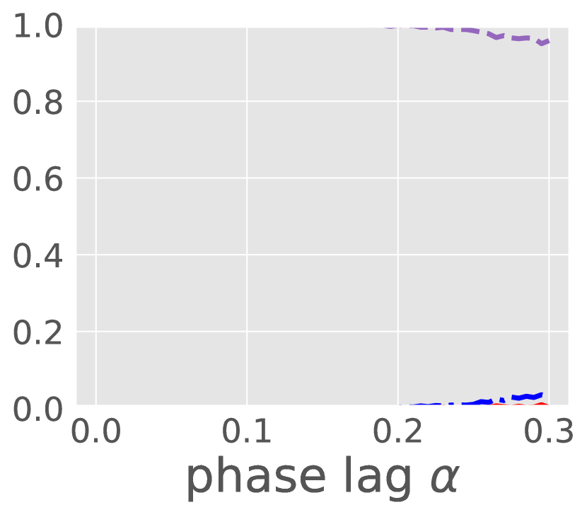
(a) ASBS

(b) Expected no. of frequency clusters

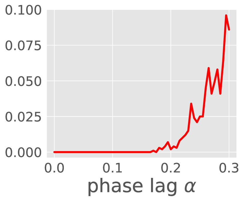
(c) Expected no. of desync oscillators

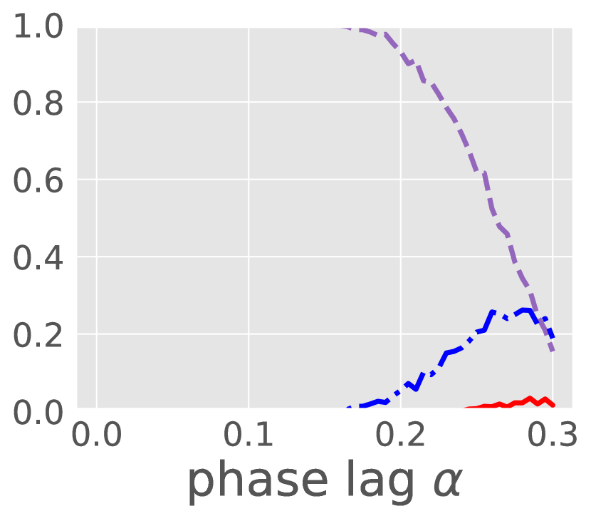
(d) global BS

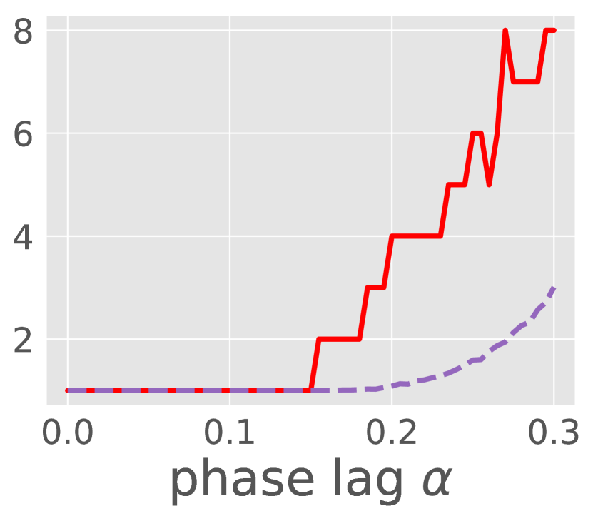
(e) Expected no. of frequency clusters

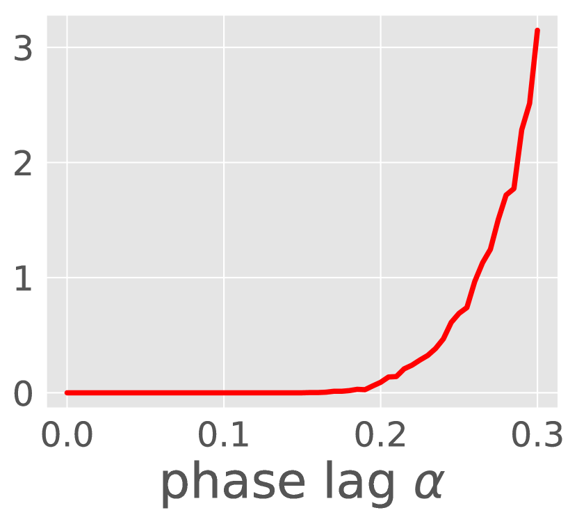
(f) Expected no. of desync oscillators