Simple Local Polynomial Density Estimators

Abstract

This paper introduces an intuitive and easy-to-implement nonparametric density estimator based on local polynomial techniques. The estimator is fully boundary adaptive and automatic, but does not require pre-binning or any other transformation of the data. We study the main asymptotic properties of the estimator, and use these results to provide principled estimation, inference, and bandwidth selection methods. As a substantive application of our results, we develop a novel discontinuity in density testing procedure, an important problem in regression discontinuity designs and other program evaluation settings. An illustrative empirical application is given. Two companion Stata and R software packages are provided.

Keywords: density estimation, local polynomial methods, regression discontinuity, manipulation test.

1 Introduction

Flexible (nonparametric) estimation of a probability density function features prominently in empirical work in statistics, economics, and many other disciplines. Sometimes the density function is the main object of interest, while in other cases it is a useful ingredient in forming two-step nonparametric or semiparametric procedures. In program evaluation and causal inference settings, for example, nonparametric density estimators are used for manipulation testing, distributional treatment effect and counterfactual analysis, instrumental variables treatment effect specification and heterogeneity analysis, and common support/overlap testing. See Imbens and Rubin (2015) and Abadie and Cattaneo (2018) for reviews and further references.

A common problem faced when implementing density estimators in empirical work is the presence of evaluation points that lie on the boundary of the support of the variable of interest: whenever the density estimator is constructed at or near boundary points, which may or may not be known by the researcher, the finite- and large-sample properties of the estimator are affected. Standard kernel density estimators are invalid at or near boundary points, while other methods may remain valid but usually require choosing additional tuning parameters, transforming the data, a priori knowledge of the boundary point location, or some other boundary-related specific information or modification. Furthermore, it is usually the case that one type of density estimator is used for evaluation points at or near the boundary, while a different type is used for interior points.

We introduce a novel nonparametric estimator of a density function constructed using local polynomial techniques (Fan and Gijbels, 1996). The estimator is intuitive, easy to implement, does not require pre-binning of the data, and enjoys all the desirable features associated with local polynomial regression estimation. In particular, the estimator automatically adapts to the boundaries of the support of the density without requiring specific data modification or additional tuning parameter choices, a feature that is unavailable for most other density estimators in the literature: see Karunamuni and Alberts (2005) for a review on this topic. The most closely related approaches currently available in the literature are the local polynomial density estimators of Cheng et al. (1997) and Zhang and Karunamuni (1998), which require knowledge of the boundary location and pre-binning of the data (or, more generally, pre-estimation of the density near the boundary), and hence introduce additional tuning parameters that need to be chosen.

The heuristic idea underlying our estimator, and differentiating it from other existing ones, is simple to explain: whereas other nonparametric density estimators are constructed by smoothing out a histogram-type estimator of the density, our estimator is constructed by smoothing out the empirical distribution function using local polynomial techniques. Accordingly, our density estimator is constructed using a preliminary tuning-parameter-free and $\sqrt{n}$-consistent distribution function estimator (where $n$ denotes the sample size), implying in particular that the only tuning parameter required by our approach is the bandwidth associated with the local polynomial fit at each evaluation point. For the resulting density estimator, we provide (i) asymptotic expansions of the leading bias and variance, (ii) asymptotic Gaussian distributional approximation and valid statistical inference, (iii) consistent standard error estimators, and (iv) consistent data-driven bandwidth selection based on an asymptotic mean squared error (MSE) expansion. All these results apply to both interior and boundary points in a fully automatic and data-driven way, without requiring boundary-specific transformations of the estimator or of the data, and without employing additional tuning parameters (beyond the main bandwidth present in any kernel-based nonparametric method).

As a substantive methodological application of our proposed density estimator, we develop a novel discontinuity in density testing procedure. In a seminal paper, McCrary (2008) proposed the idea of manipulation testing via discontinuity in density testing for regression discontinuity (RD) designs, and developed an implementation thereof using the density estimator of Cheng et al. (1997), which requires pre-binning of the data and choosing two tuning parameters. On the other hand, the new proposed discontinuity in density test employing our density estimator only requires the choice of one tuning parameter, and enjoys other features associated with local polynomials methods. We also illustrate its performance with an empirical application employing the canonical Head Start data in the context of RD designs (Ludwig and Miller, 2007). For introductions to RD designs, and further references, see Imbens and Lemieux (2008), Lee and Lemieux (2010), and Cattaneo et al. (2017). For recent papers on modern RD methodology see, for example, Arai and Ichimura (2018), Ganong and Jäger (2018), Hyytinen et al. (2018), Dong et al. (2019), and references therein.

Finally, we provide two general purpose software packages, for Stata and R, implementing the main results discussed in the paper. Cattaneo et al. (2018) discusses the package rddensity, which is specifically tailored to manipulation testing (i.e., two-sample discontinuity in density testing), while Cattaneo et al. (2019) discusses the package lpdensity, which provides generic density estimation over the support of the data.

The rest of the paper is organized as follows. Section 2 introduces the density estimator and Section 3 gives the main technical results. Section 4 applies these results to nonparametric discontinuity in density testing (i.e., manipulation testing), while Section 5 illustrates the new method with an empirical application. Section 6 discusses extensions and concludes. The supplemental appendix (SA hereafter) contains additional methodological and technical results and reports all theoretical proofs. In addition, to conserve space, we relegate to the SA and to our two companion software articles the presentation of simulation evidence highlighting the finite sample properties of our proposed density estimator.

2 Boundary Adaptive Density Estimation

Suppose $\{x_{1},x_{2},\cdots,x_{n}\}$ is a random sample, where $x_{i}$ is a continuous random variable with a smooth cumulative distribution function over its support $\mathcal{X}\subseteq\mathbb{R}$. The probability density function is $f(x)=\frac{\partial}{\partial x}\mathbb{P}[x_{i}\leq x]$, where the derivative is interpreted as a one-sided derivative at a boundary point of $\mathcal{X}$. Our results apply to bounded or unbounded support $\mathcal{X}$, which is an important feature in empirical applications employing density estimators.

Letting $\hat{F}(x)=\frac{1}{n}\sum_{i=1}^{n}{\rm 1\rule{0.43057pt}{6.54443pt}\hskip 0.86108pt}(x_{i}\leq x)$ denote the classical empirical distribution function, our proposed local polynomial density estimator is

$$\hat{f}(x)=\mathbf{e}_{1}^{\prime}\mathbf{\hat{\beta}}(x),\qquad\mathbf{\hat{\beta}}(x)=\underset{\mathbf{b}\in\mathbb{R}^{p+1}}{\operatorname{argmin}}\sum_{i=1}^{n}\left[\hat{F}(x_{i})-\mathbf{r}_{p}(x_{i}-x)^{\prime}\mathbf{b}\right]^{2}K\left(\frac{x_{i}-x}{h}\right),$$

where $\mathbf{e}_{1}=(0,1,0,\cdots,0)^{\prime}$ is the second $(p+1)$-dimensional unit vector, $\mathbf{r}_{p}(u)=(1,u,u^{2},\cdots,u^{p})^{\prime}$ is a $p$-th order polynomial expansion, $K(\cdot)$ denotes a kernel function, $h$ is a positive bandwidth, and $p\geq 1$. In other words, we take the empirical distribution function $\hat{F}$ as the starting point, then construct a smooth local approximation to $\hat{F}$ using a polynomial expansion, and finally obtain the density estimator $\hat{f}$ as the slope coefficient in the local polynomial regression.

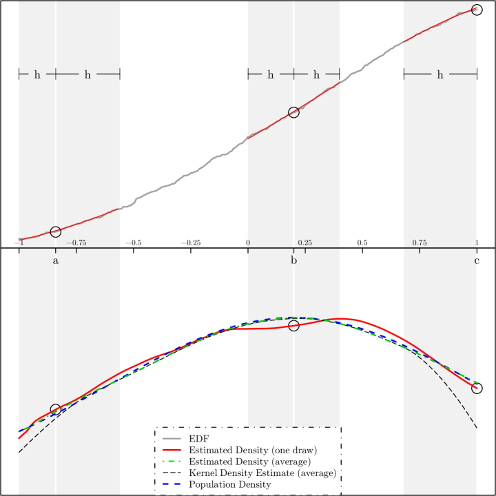
Figure 1: Graphical Illustration of Density Estimator.

The idea behind the density estimator $\hat{f}(x)$ is explained graphically in Figure 1. In this figure, we consider three distinct evaluation points on $\mathcal{X}=[-1,1]$: $a$ is near the lower boundary, $b$ is an interior point, and $c=1$ is the upper boundary. The conventional kernel density estimator, $\hat{f}_{\mathtt{KD}}(x)=\frac{1}{nh}\sum_{i=1}^{n}K\left(\frac{x_{i}-x}{h}\right)$, is valid for interior points, but otherwise inconsistent. See, e.g., Wand and Jones (1995) for a classical reference. On the other hand, our density estimator $\hat{f}(x)$ is valid for all evaluation points $x\in\mathcal{X}$ and can be used directly, without any modifications to approximate the unknown density. Figure 1 is constructed using $n=500$ observations. The top panel plots one realization of the empirical distribution function $\hat{F}(x)$ in dark gray, and the local polynomial fits for the three evaluation points $x\in\{a,b,c\}$ in red, the latter implemented with $p=2$ (quadratic approximation) and bandwidth $h$ (different value for each evaluation point considered). The vertical light gray areas highlight the localization region controlled by the bandwidth choice, that is, only observations falling in these regions are used to smooth out the empirical distribution function via local polynomial approximation, depending on the evaluation point. The estimator $\hat{f}(x)$ is the slope coefficient accompanying the first-order term in the local polynomial approximation, which is depicted in the bottom panel of Figure 1 as the solid line in red. The bottom panel also plots three other curves: dashed blue line corresponding to the population density function, dash-dotted green line corresponding to the average of our density estimate over simulations, and dashed black line corresponding to the average of the standard kernel density estimates $\hat{f}_{\mathtt{KD}}(x)$.

Figure 1 illustrates how our proposed density estimator adapts to (near) boundary points automatically, showing graphically its good performance in repeated samples. Evaluation point $b$ is an interior point and, consequently, a symmetric smoothing around that point is employed, just like the standard estimator $\hat{f}_{\mathtt{KD}}(x)$ does. On the other hand, evaluation points $a$ and $c$ both exhibit boundary bias if the standard kernel density estimator is used: point $a$ is near the boundary and hence employs asymmetric smoothing, while point $c$ is at the upper boundary and hence employs one-sided smoothing. In contrast, our proposed density estimator $\hat{f}(x)$ automatically adapts to the boundary point, as the bottom panel in Figure 1 illustrates.

3 Main Technical Results

We summarize two main large sample results concerning the proposed density estimator: (i) an asymptotic distributional approximation with precise leading bias and variance characterizations, and (ii) a consistent standard error estimator, which is also data-driven and fully automatic. Both results are boundary adaptive and do not require prior knowledge of the shape of $\mathcal{X}$. We report preliminary technical lemmas, additional theoretical results, and detailed proofs in the SA to conserve space. Extensions and other applications of our methods are mentioned in Section 6.

Assumption 1 (DGP)

$\{x_{1},x_{2},\cdots,x_{n}\}$ is a random sample with distribution function $F$ that is $p+1$ times continuously differentiable for some $p\geq 1$ in a neighborhood of the evaluation point $x$, and the probability density function of $x_{i}$, denoted by $f$, is positive at $x$.

This assumption imposes basic regularity conditions on the data generating process, ensuring that $f(x)$ is well-defined and possesses enough smoothness.

Assumption 2 (Kernel)

The kernel function $K(\cdot)$ is nonnegative, symmetric, and continuous on its support $[-1,1]$.

This assumption is standard in nonparametric estimation, and is satisfied for common kernel functions. We exclude kernels with unbounded support (e.g., Gaussian kernel) for simplicity, since such kernels will always hit boundaries. Our results, however, can be extended to accommodate kernel functions with unbounded support, albeit more cumbersome notation would be needed.

The following theorem gives a characterization of the asymptotic bias and variance of $\hat{f}(x)$, as well as a valid distributional approximation. All limits are taken as $n\rightarrow\infty$ (and $h\rightarrow 0$) unless explicitly stated otherwise, $\rightsquigarrow$ denotes weak convergence, and $F^{(s)}(x)=\partial^{s}F(x)/\partial x^{s}$ denotes the derivative, or one-sided derivative if at a boundary point, of $F(x).$

Theorem 1 (Distributional Approximation)

Suppose Assumption 1 and 2 hold. If $nh^{2}\rightarrow\infty$ and $nh^{2p+1}=O(1)$, then

$$\frac{\hat{f}(x)-f(x)-h^{p}\mathcal{B}(x)}{\sqrt{\frac{1}{nh}\mathcal{V}(x)}}\rightsquigarrow\mathcal{N}(0,1),$$

where, defining

$$\mathbf{A}(x) =f(x)\int_{h^{-1}(\mathcal{X}-x)}\mathbf{r}_{p}(u)\mathbf{r}_{p}(u)^{\prime}K(u)\mathrm{d}u,\qquad\mathbf{a}(x)=f(x)\frac{F^{(p+1)}(x)}{(p+1)!}\int_{h^{-1}(\mathcal{X}-x)}u^{p+1}\mathbf{r}_{p}(u)K(u)\mathrm{d}u,$$

$$\mathbf{B}(x) =f(x)^{3}\iint_{h^{-1}(\mathcal{X}-x)}\min\{u,v\}\mathbf{r}_{p}(u)\mathbf{r}_{p}(v)^{\prime}K(u)K(v)\text{d}u\mathrm{d}v,$$

the asymptotic bias and variance are $\mathcal{B}(x)=\mathbf{e}_{1}^{\prime}\mathbf{A}(x)^{-1}\mathbf{a}(x)$ and $\mathcal{V}(x)=\mathbf{e}_{1}^{\prime}\mathbf{A}(x)^{-1}\mathbf{B}(x)\mathbf{A}(x)^{-1}\mathbf{e}_{1}$, respectively.

In this theorem, the integration region reflects the effect of boundaries. Because $K(\cdot)$ is compactly supported, if $x$ is an interior point, we have $h^{-1}(\mathcal{X}-x)\supset[-1,1]$ for $h$ small enough, thus ensuring the kernel function is not truncated and the local approximation is symmetric around $x$. On the other hand, for $x$ near or at a boundary of $\mathcal{X}$ (i.e., for $h$ not small enough relative to the distance of $x$ to the boundary), we have $h^{-1}(\mathcal{X}-x)\not\supset[-1,1]$, and the local approximation is asymmetric (or one-sided). It follows that the density estimator $\hat{f}(x)$ is boundary adaptive and design adaptive, as in the case of local polynomial regression (Fan and Gijbels, 1996).

A simple and automatic variance estimator is $\hat{\mathcal{V}}(x)=\mathbf{e}_{1}^{\prime}\mathbf{\hat{A}}(x)^{-1}\mathbf{\hat{B}}(x)\mathbf{\hat{A}}(x)^{-1}\mathbf{e}_{1}$, where

$$\hat{\mathbf{A}}(x) =\frac{1}{nh}\sum_{i=1}^{n}\mathbf{r}_{p}\left(\check{x}_{i}\right)\mathbf{r}_{p}\left(\check{x}_{i}\right)^{\prime}K\left(\check{x}_{i}\right)$$

$$\hat{\mathbf{B}}(x) =\frac{1}{n^{3}h^{3}}\sum_{i,j,k=1}^{n}\mathbf{r}_{p}\left(\check{x}_{j}\right)\mathbf{r}_{p}\left(\check{x}_{k}\right)^{\prime}K\left(\check{x}_{j}\right)K\left(\check{x}_{k}\right)\left[{\rm 1\rule{0.43057pt}{6.54443pt}\hskip 0.86108pt}(x_{i}\leq x_{j})-\hat{F}(x_{j})\right]\left[{\rm 1\rule{0.43057pt}{6.54443pt}\hskip 0.86108pt}(x_{i}\leq x_{k})-\hat{F}(x_{k})\right],$$

with $\check{x}_{i}=h^{-1}(x_{i}-x)$ denoting the normalized observations to save notation. Let $\rightarrow_{\mathbb{P}}$ denote convergence in probability.

Theorem 2 (Variance Estimation)

If the conditions in Theorem 1 hold, then $\hat{\mathcal{V}}(x)\rightarrow_{\mathbb{P}}\mathcal{V}(x)$.

As shown in this theorem, the variance estimator $\hat{\mathcal{V}}(x)$ does not require knowledge of the relative positioning of the evaluation point to boundaries of $\mathcal{X}$, that is, $\hat{\mathcal{V}}(x)$ is also boundary adaptive. A boundary adaptive bias estimator $\mathcal{\hat{B}}(x)$ can also be constructed easily, as shown in the SA.

Using the results above, and under mild regularity conditions, it follows that a pointwise approximate MSE-optimal bandwidth choice for our proposed density estimator $\hat{f}(x)$ is

$$h_{\mathtt{MSE}}(x)=\left(\frac{\mathcal{V}(x)}{2p\mathcal{B}(x)^{2}}\right)^{1/(1+2p)}n^{-1/(1+2p)}\text{,}$$

which can be easily implemented by replacing $\mathcal{B}(x)$ and $\mathcal{V}(x)$ with preliminary consistent estimators $\mathcal{\hat{B}}(x)$ and $\mathcal{\hat{V}}(x)$. The SA offers details on implementation and consistency of this MSE-optimal bandwidth selector, which can be used to establish its optimality in the sense of Li (1987), and also bandwidth selection for estimating higher-order density derivatives. We omit these results here due to space limitations.

Finally, we recommend implementing the density estimator $\hat{f}(x)$ with $p=2$, which corresponds to the minimal odd polynomial order choice (i.e., analogous to local linear regression). Higher-order local polynomials could be used, but they typically exhibit erratic behavior near boundary points, and lead to counter-intuitive weighting schemes. See (Fan and Gijbels, 1996, Chapter 3.3) for an automatic polynomial order selection methods that can be applied to our estimator as well.

4 Application to Manipulation Testing

Testing for manipulation is useful when units are assigned to two (or more) distinct groups using a hard-thresholding rule based on an observable variable, as it provides an intuitive and simple method to check empirically whether units are able to alter (i.e., manipulate) their assignment. Manipulation tests are used in empirical work both as falsification tests of regression discontinuity (RD) designs and as empirical tests with substantive implications in other program evaluation settings. Available methods from the RD literature include the original implementation of McCrary (2008) based on Cheng et al. (1997), the empirical likelihood testing procedure of Otsu et al. (2014) based on boundary-corrected kernels, and the finite sample binomial test presented in Cattaneo et al. (2017) based on local randomization ideas.

In this section, we introduce a new manipulation testing procedure based on our proposed local polynomial density estimator. Our method requires choosing only one tuning parameter, avoids pre-binning the data, and permits the use of simple well-known weighting schemes (e.g., uniform or triangular kernel), thereby avoiding the need of choosing the length and positions of bins for pre-binning or employing more complicated boundary kernels. In addition, our method is intuitive, easy-to-implement, and fully data-driven: bandwidth selection methods are formally developed and implemented, along with valid inference methods based on robust bias correction.

To describe the manipulation testing setup, suppose units are assigned to one group (“control”) if $x_{i}<\bar{x}$ and to another group (“treatment”) if $x_{i}\geq\bar{x}$. For example, in the application discussed below, we employ the Head Start data, where $x_{i}$ is a poverty index at the county level, $\bar{x}=59.1984$ is a fixed cutoff determining eligibility to the program. The goal is to test formally whether the density $f(x)$ is continuous at $\bar{x}$, using the two subsamples $\{x_{i}:x_{i}<\bar{x}\}$ and $\{x_{i}:x_{i}\geq\bar{x}\}$, and thus the null and alternative hypotheses are:

$$\mathsf{H}_{0}:\lim_{x\uparrow\bar{x}}f(x)=\lim_{x\downarrow\bar{x}}f(x)\qquad\text{vs}\qquad\mathsf{H}_{1}:\lim_{x\uparrow\bar{x}}f(x)\neq\lim_{x\downarrow\bar{x}}f(x).$$

This hypothesis testing problem induces a nonparametric boundary point at $x=\bar{x}$ because two distinct densities need to be estimated, one from the left and the other from the right. Our proposed density estimator $\hat{f}(x)$ is readily applicable because it is boundary adaptive and fully automatic, and it can also be used to plot the density near the cutoff in an automatic way: see Figure 2 below for an example using the Head Start data.

Let $\hat{F}_{-}$ and $\hat{F}_{+}$ be the empirical distribution functions constructed using only units with $x_{i}<\bar{x}$ and with $x_{i}\geq\bar{x}$, respectively. Then, $\hat{f}$ can be applied twice, to the data below and above the cutoff, to obtain two estimators of the density at the boundary point $\bar{x}$, which we denote by $\hat{f}_{-}(\bar{x})$ and $\hat{f}_{+}(\bar{x})$, respectively. Thus, our proposed manipulation test statistic takes the form:

$$T_{p}(h)=\frac{\frac{n_{+}}{n}\hat{f}_{+}(\bar{x})-\frac{n_{-}}{n}\hat{f}_{-}(\bar{x})}{\sqrt{\frac{n_{+}}{n}\frac{1}{nh_{+}}\mathcal{\hat{V}}_{+}(\bar{x})+\frac{n_{-}}{n}\frac{1}{nh_{-}}\mathcal{\hat{V}}_{-}(\bar{x})}},$$

where $n_{-}=\sum_{i=1}^{n}{\rm 1\rule{0.43057pt}{6.54443pt}\hskip 0.86108pt}(x_{i}<x)$ and $n=n_{-}+n_{+}$, $\mathcal{\hat{V}}_{-}(x)$ and $\mathcal{\hat{V}}_{+}(x)$ denote the variance estimators mentioned previously but now computed for the two subsamples $x_{i}<\bar{x}$ and $x_{i}\geq\bar{x}$, respectively, and $h_{-}$ and $h_{+}$ denote the bandwidths used below and above $\bar{x}$. Employing our main theoretical results, we provide precise conditions so that the finite sample distribution of $T_{p}(h)$ can be approximated by the standard normal distribution, which leads to the following result: under the regularity conditions given above, and if $n\min\{h_{-}^{2},h_{+}^{2}\}\rightarrow\infty$ and $n\max\{h_{-}^{1+2p},h_{+}^{1+2p}\}\rightarrow 0$, then

$$\text{Under }\mathsf{H}_{0} :\lim_{n\rightarrow\infty}\mathbb{P}[|T_{p}(h)|\geq\Phi_{1-\alpha/2}]=\alpha,$$

$$\text{Under }\mathsf{H}_{1} :\lim_{n\rightarrow\infty}\mathbb{P}[|T_{p}(h)|\geq\Phi_{1-\alpha/2}]=1,$$

where $\Phi_{\alpha}$ denotes the $\alpha$-quantile of the standard Gaussian distribution, $\alpha\in(0,1)$. This establishes asymptotic validity and consistency of the $\alpha$-level testing procedure that rejects $\mathsf{H}_{0}$ iff $|T(h)|\geq\Phi_{1-\alpha/2}$. The SA includes detailed proofs, and related implementation details.

A key implementation issue of our manipulation test is the choice of bandwidth $h$, a problem common to all nonparametric manipulation tests available in the literature. To select $h$ in an automatic and data-driven way, we obtain an approximate MSE-optimal bandwidth choice for the point estimator $\hat{f}_{+}(\bar{x})-\hat{f}_{-}(\bar{x})$, and then propose a consistent implementation thereof, which is denoted by $\hat{h}_{p}$. We give the details in the SA, where we also present alternative MSE-optimal bandwidth selectors for each-side density estimator separately. Given the data-driven bandwidth choice $\hat{h}_{p}$, or its theoretical (infeasible) counterpart $h_{p}$, we propose a simple robust bias-corrected test statistic implementation following ideas in Calonico et al. (2014) and Calonico et al. (2018); see the latter reference for theoretical results on higher-order refinements and the important role of pre-asymptotic variance estimation in the context of local polynomial regression estimation. Specifically, our proposed data-driven robust bias-corrected test statistic is $T_{p+1}(\hat{h}_{p})$, which rejects $\mathsf{H}_{0}$ iff $|T_{p+1}(\hat{h}_{p})|\geq\Phi_{1-\alpha/2}$ for a nominal $\alpha$-level test. This approach corresponds to a special case of manual bias-correction together with the corresponding adjustment of Studentization. A natural choice is $p=2$, and this is the default in our companion Stata and R software implementations.

5 Empirical Illustration

We apply our manipulation test to the data of Ludwig and Miller (2007) on the original Head Start implementation in the U.S. In this empirical application, a discontinuity on access to program funds at the county level occurred in $1965$ when the program was first implemented: the federal government provided grant writing assistance to the $300$ poorest counties as measured by a poverty index, which was computed in $1965$ using $1960$ Census variables, thus creating a discontinuity in program elegibility. Using our notation, $x_{i}$ denotes the poverty index for county $i$, and $\bar{x}=59.1984$ is the cutoff point (i.e., the poverty index of the $300$-th poorest municipality).

A manipulation test in this context amounts to testing whether there is a disproportional number of counties are situated above $\bar{x}$ relative to those present below the cutoff. Figure 2 presents the histogram of counties below and above the cutoff together with our local polynomial density estimate and associated pointwise robust bias-corrected confidence intervals over a grid of points near the cutoff $\bar{x}$, implemented using $p=2$ and the MSE-optimal data-driven bandwidth estimate. Table 1 presents the empirical results from our manipulation test. We consider two main approaches, both covered by our theoretical work and available in our software implementation: (i) using two distinct bandwidths on each side of the cutoff ($h_{-}\neq h_{+}$), and (ii) using a common bandwidth for each side of the cutoff ($h_{-}=h_{+}$), with $h_{-}$ and $h_{+}$ denoting the bandwidth on the left and on the right, respectively. For each case, we consider three distinct implementations of our manipulation test, which varies the degree of polynomial approximation used to smooth out the empirical distribution function: $T_{q}(h_{p})$ denotes the test statistic constructed using a $q$-th order local polynomial density estimator, with bandwidth choice that is MSE-optimal for $p$-th order local polynomial density estimator. For example, our recommended choice is $T_{3}(h_{2})$, with either common bandwidth or two different bandwidths, which amounts to first choosing MSE-optimal bandwidth(s) for a local quadratic fit, and then conducting inference using a cubic approximation. This approach is the simplest implementation of the robust bias correction inference: $T_{p}(h_{p})$ does not lead to a valid inference approach because a first-order bias will make the test over-reject the null hypothesis. We also report the original implementation of the McCrary test for comparison.

Our empirical results show no evidence of manipulation. In fact, this finding is consistent with the underlying institutional knowledge of the program: the poverty index was constructed in $1965$ at the federal level using county level information from the $1960$ Census, which implies it is indeed highly implausible that individual counties could have manipulated their assigned poverty index. Our findings are robust to different bandwidth and local polynomial order specifications. Finally, we note two theory-based empirical findings: (i) our proposed manipulation test employs robust bias-corrected methods, and hence leads to asymmetric confidence intervals (not necessarily centered around the density point estimator); and (ii) the effective sample size of the original McCrary test is much smaller than our proposed manipulation test because of the pre-binning of the data, and hence can lead to important reduction in power of the test.

6 Conclusion

We introduced a boundary adaptive kernel-based density estimator employing local polynomial methods, which requires choosing only one tuning parameter and does not require boundary-specific data transformations (such as pre-binning). We studied the main asymptotic properties of the estimator, and used these results to developed a new manipulation test via discontinuity in density testing. Several extensions and generalizations of our results are underway in ongoing work, and two distinct general purpose software packages in Stata and R are readily available Cattaneo et al. (2018, 2019).

Notes: (i) Constructed using companion R (and Stata) package described in Cattaneo et al. (2019) with simulated data.

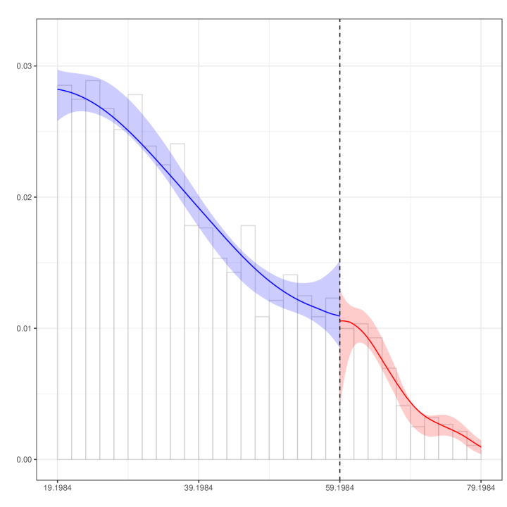
Figure 2: Manipulation Testing, Head Start Data.

Notes: (i) Histogram estimate (light grey in background) of the running variable (poverty index) computed with default values in R; (ii) local polynomial density estimate (solid blue and red) and robust bias corrected confidence intervals (shaded blue and red) computed using companion R (and Stata) package described in Cattaneo et al. (2018); and (ii) $n_{-}=2,504$, $n_{+}=300$, and $\bar{x}=59.1984$.

Table 1: Manipulation Testing, Head Start Data.

	Pre-binning			Bandwidths			Eff. $n$			Test
	left	right		left	right		left	right		$T$	$p$-val
$h_{-}\neq h_{+}$
$T_{2}(\hat{h}_{1})$				$15.771$	$2.326$		$581$	$65$		$0.024$	$0.981$
$T_{3}(\hat{h}_{2})$				$19.776$	$8.296$		$762$	$210$		$-1.146$	$0.252$
$T_{4}(\hat{h}_{3})$				$32.487$	$10.808$		$1598$	$232$		$-1.083$	$0.279$
$h_{-}=h_{+}$
$T_{2}(\hat{h}_{1})$				$3.274$	$3.274$		$99$	$95$		$-1.355$	$0.175$
$T_{3}(\hat{h}_{2})$				$9.213$	$9.213$		$316$	$221$		$-0.515$	$0.607$
$T_{4}(\hat{h}_{3})$				$12.270$	$12.270$		$419$	$243$		$-0.712$	$0.477$
McCrary	$76$	$60$		$13.950$	$13.950$		$24$	$24$		$0.142$	$0.887$

Notes: (i) $T_{p}(h)$ denotes the manipulation test statistic using $p$-th order density estimators with bandwidth choice $h$ (which could be common on both sides or different on either side of the cutoff), and $\hat{h}_{p}$ denotes the estimated MSE-optimal bandwidths for $p$-th order density estimator or difference of estimators (depending on the case considered); (ii) Columns under “Bandwidths” report estimated MSE-optimal bandwidths, Columns under “Eff. $n$” report effective sample size on either side of the cutoff, and Columns under “Test” report value of test statistic ($T$) and two-sided p-value ($p$-val); (iii) first three rows allow for different bandwidths on each side of the cutoff, while the next three rows employ a common bandwidth on both sides of the cutoff (chosen to be MSE-optimal for the difference of density estimates). All estimates are obtained using companion R (and Stata) package described in Cattaneo et al. (2018); and (iv) the last row, labeled “McCrary”, corresponds to the original implementation of McCrary (2008), and therefore columns under “Pre-binning” report the total number of bins used for pre-bining of the data and columns under “Eff. $n$” report the number of bins used for local linear density estimation.

References

- Abadie and Cattaneo (2018) Abadie, A., and Cattaneo, M. D. (2018), “Econometric Methods for Program Evaluation,” Annual Review of Economics, 10, 465–503.
- Arai and Ichimura (2018) Arai, Y., and Ichimura, H. (2018), “Simultaneous Selection of Optimal Bandwidths for the Sharp Regression Discontinuity Estimator,” Quantitative Economics, 9, 441–482.
- Calonico et al. (2018) Calonico, S., Cattaneo, M. D., and Farrell, M. H. (2018), “On the Effect of Bias Estimation on Coverage Accuracy in Nonparametric Inference,” Journal of the American Statistical Association, 113, 767–779.
- Calonico et al. (2014) Calonico, S., Cattaneo, M. D., and Titiunik, R. (2014), “Robust Nonparametric Confidence Intervals for Regression-Discontinuity Designs,” Econometrica, 82, 2295–2326.
- Cattaneo et al. (2018) Cattaneo, M. D., Jansson, M., and Ma, X. (2018), “Manipulation Testing based on Density Discontinuity,” Stata Journal, 18, 234–261.
- Cattaneo et al. (2019) (2019), “lpdensity: Local Polynomial Density Estimation and Inference,” working paper.
- Cattaneo et al. (2017) Cattaneo, M. D., Titiunik, R., and Vazquez-Bare, G. (2017), “Comparing Inference Approaches for RD Designs: A Reexamination of the Effect of Head Start on Child Mortality,” Journal of Policy Analysis and Management, 36, 643–681.
- Cheng et al. (1997) Cheng, M.-Y., Fan, J., and Marron, J. S. (1997), “On Automatic Boundary Corrections,” Annals of Statistics, 25, 1691–1708.
- Dong et al. (2019) Dong, Y., Lee, Y.-Y., and Gou, M. (2019), “Regression Discontinuity Designs with a Continuous Treatment,” SSRN working paper No. 3167541.
- Fan and Gijbels (1996) Fan, J., and Gijbels, I. (1996), Local Polynomial Modelling and Its Applications, New York: Chapman & Hall/CRC.
- Ganong and Jäger (2018) Ganong, P., and Jäger, S. (2018), “A Permutation Test for the Regression Kink Design,” Journal of the American Statistical Association, 113, 494–504.
- Hyytinen et al. (2018) Hyytinen, A., Meriläinen, J., Saarimaa, T., Toivanen, O., and Tukiainen, J. (2018), “When Does Regression Discontinuity Design Work? Evidence from Random Election Outcomes,” Quantitative Economics, 9, 1019–1051.
- Imbens and Lemieux (2008) Imbens, G., and Lemieux, T. (2008), “Regression Discontinuity Designs: A Guide to Practice,” Journal of Econometrics, 142, 615–635.
- Imbens and Rubin (2015) Imbens, G. W., and Rubin, D. B. (2015), Causal Inference in Statistics, Social, and Biomedical Sciences, Cambridge University Press.
- Karunamuni and Alberts (2005) Karunamuni, R., and Alberts, T. (2005), “On Boundary Correction in Kernel Density Estimation,” Statistical Methodology, 2, 191–212.
- Lee and Lemieux (2010) Lee, D. S., and Lemieux, T. (2010), “Regression Discontinuity Designs in Economics,” Journal of Economic Literature, 48, 281–355.
- Li (1987) Li, K.-C. (1987), “Asymptotic Optimality for , , Cross-validation and Generalized Cross-validation: Discrete Index Set,” Annals of Statistics, 15, 958–975.
- Ludwig and Miller (2007) Ludwig, J., and Miller, D. L. (2007), “Does Head Start Improve Children’s Life Chances? Evidence from a Regression Discontinuity Design,” Quarterly Journal of Economics, 122, 159–208.
- McCrary (2008) McCrary, J. (2008), “Manipulation of the Running Variable in the Regression Discontinuity Design: A Density Test,” Journal of Econometrics, 142, 698–714.
- Otsu et al. (2014) Otsu, T., Xu, K.-L., and Matsushita, Y. (2014), “Estimation and Inference of Discontinuity in Density,” Journal of Business and Economic Statistics, 31, 507–524.
- Wand and Jones (1995) Wand, M., and Jones, M. (1995), Kernel Smoothing, Florida: Chapman & Hall/CRC.
- Zhang and Karunamuni (1998) Zhang, S., and Karunamuni, R. J. (1998), “On Kernel Density Estimation Near Endpoints,” Journal of Statistical Planning and Inference, 70, 301–316.