Topological optimization via cost penalization

Abstract

We consider general shape optimization problems governed by Dirichlet boundary value problems. The proposed approach may be extended to other boundary conditions as well. It is based on a recent representation result for implicitly defined manifolds, due to the authors, and it is formulated as an optimal control problem. The discretized approximating problem is introduced and we give an explicit construction of the associated discrete gradient. Some numerical examples are also indicated.

Keywords: geometric optimization; optimal design; topological variations; optimal control methods; discrete gradient

1 Introduction

Shape optimization is a relatively young branch of mathematics, with important modern applications in engineering and design. Certain optimization problems in mechanics, thickness optimization for plate or rods, geometric optimization of shells, curved rods, drag minimization in fluid mechanics, etc are some examples. Many appear naturally in the form of control by coefficients problems, due to the formulation of the mechanical models, with the geometric characteristics entering the coefficients of the differential operators. See [15], Ch. 6, where such questions are discussed in details.

It is the aim of this article to develop an optimal control approach, using penalization methods, to general shape optimization problems as investigated in [20], [23], [5], [10], [8], etc. We underline that our methodology allows simultaneous topological and boundary variations.

Here, we fix our attention on the case of Dirichlet boundary conditions and we study the typical problem (denoted by ($\mathcal{P}$)):

$$\min_{\Omega}\int_{E}j\left(\mathbf{x},y_{\Omega}(\mathbf{x})\right)d\mathbf{x},$$ (1.1)

$$-\Delta y_{\Omega}=f\hbox{ in }\Omega,$$ (1.2)

$$y_{\Omega}=0\hbox{ on }\partial\Omega,$$ (1.3)

where $E\subset\subset D\subset\mathbb{R}^{2}$ are given bounded domains, $D$ is of class $\mathcal{C}^{1,1}$ and the minimization parameter, the unknown domain $\Omega$, satisfies $E\subset\Omega\subset D$ and other possible conditions defining a class of admissible domains. Notice that the case of dimension two is of interest in shape optimization. Moreover, $f\in L^{2}(D)$, $j:D\times\mathbb{R}\rightarrow\mathbb{R}$ is some Carathéodory mapping. More assumptions or constraints will be imposed later. Other boundary conditions or differential operators may be handled as well via this control approach and we shall examine such questions in a subsequent paper.

For fundamental properties and methods in optimal control theory, we quote [12], [7], [2], [16]. The problem (1.1)-(1.3) and its approximation are strongly non convex and challenging both from the numerical and theoretical points of view. The investigation from this paper continues the one in [26] and is essentially based on the recent implicit parametrization method as developed in [25], [18], [24], that provides an efficient analytic representation of the unknown domains.

The Hamiltonian approach to implicitly defined manifolds will be briefly recalled together with other preliminaries in Section 2. The precise formulation of the problem and its approximation is analyzed in Section 3 together with its differentiability properties. In Section 4, we study the discretized version and find the general form of the discrete gradient. The last section is devoted to some numerical experiments, using this paper approach.

The method studied in this paper has a certain complexity due to the use of Hamiltonian systems and its main advantage is the possibility to extend it to other boundary conditions or boundary observation problems. This will be performed in a subsequent article.

2 Preliminaries

Consider the Hamiltonian system

$$x_{1}^{\prime}(t) = -\frac{\partial g}{\partial x_{2}}\left(x_{1}(t),x_{2}(t)\right),\quad t\in I,$$ (2.1)

$$x_{2}^{\prime}(t) = \frac{\partial g}{\partial x_{1}}\left(x_{1}(t),x_{2}(t)\right),\quad t\in I,$$ (2.2)

$$\left(x_{1}(0),x_{2}(0)\right) = \left(x_{1}^{0},x_{2}^{0}\right),$$ (2.3)

where $g:D\rightarrow\mathbb{R}$ is in $\mathcal{C}^{1}(\overline{D})$, $\left(x_{1}^{0},x_{2}^{0}\right)\in D$ and $I$ is the local existence interval for (2.1)–(2.3), around the origin, obtained via the Peano theorem. The conservation property [24] of the Hamiltonian gives:

Proposition 2.1

We have

$$g\left(x_{1}(t),x_{2}(t)\right)=g\left(x_{1}^{0},x_{2}^{0}\right),\quad t\in I.$$ (2.4)

In the sequel, we assume that

$$g\left(x_{1}^{0},x_{2}^{0}\right)=0,\quad\nabla g\left(x_{1}^{0},x_{2}^{0}\right)\neq 0.$$ (2.5)

Under condition (2.5), i.e. in the noncritical case, it is known that the solution of (2.1)–(2.3) is also unique (by applying the implicit functions theorem to (2.4), [4]).

Remark 2.1

In higher dimension, iterated Hamiltonian systems were introduced in [25] and uniqueness and regularity properties are proved. Some relevant examples in dimension three are discussed in [18]. In the critical case, generalized solutions can be obtained [24], [25].

We define now the family $\mathcal{F}$ of admissible functions $g\in\mathcal{C}^{2}(\overline{D})$ that satisfy the conditions:

$$g(x_{1},x_{2}) > 0,\quad\hbox{on }\partial D,$$ (2.6)

$$|\nabla g(x_{1},x_{2})| > 0,\quad\hbox{on }\mathcal{G}=\left\{(x_{1},x_{2})\in D;\ g(x_{1},x_{2})=0\right\},$$ (2.7)

$$g(x_{1},x_{2}) < 0,\quad\hbox{on }\overline{E}.$$ (2.8)

Condition (2.6) says that $\mathcal{G}\cap\partial D=\emptyset$ and condition (2.7) is an extension of (2.5). In fact, it is related to the hypothesis on the non existence of equilibrium points in the Poincare-Bendixson theorem, [11], Ch. 10, and the same is valid for the next proposition. The family $\mathcal{F}$ defined by (2.6)–(2.8) is obviously very rich, but it is not “closed” (we have strict inequalities). Our approach here, gives a descent algorithm for the shape optimization problem ($\mathcal{P}$) and existence of optimal shapes is not discussed.

Following [26], we have the following two propositions:

Proposition 2.2

Under hypotheses (2.6), (2.7), $\mathcal{G}$ is a finite union of closed curves of class $\mathcal{C}^{2}$, without self intersections, parametrized by (2.1)–(2.3), when some initial point $(x_{1}^{0},x_{2}^{0})$ is chosen on each component of $\mathcal{G}$.

If $r\in\mathcal{F}$ as well, we define the perturbed set

$$\mathcal{G}_{\lambda}=\left\{(x_{1},x_{2})\in D;\ (g+\lambda r)(x_{1},x_{2})=0,\ \lambda\in\mathbb{R}\right\}.$$ (2.9)

We also introduce the neighborhood $V_{\epsilon}$, $\epsilon>0$

$$V_{\epsilon}=\left\{(x_{1},x_{2})\in D;\ d[(x_{1},x_{2}),\mathcal{G}]<\epsilon\right\},$$ (2.10)

where $d[(x_{1},x_{2}),\mathcal{G}]$ is the distance from a point to $\mathcal{G}$.

Proposition 2.3

If $\epsilon>0$ is small enough, there is $\lambda(\epsilon)>0$ such that, for $|\lambda|<\lambda(\epsilon)$ we have $\mathcal{G}_{\lambda}\subset V_{\epsilon}$ and $\mathcal{G}_{\lambda}$ is a finite union of class $\mathcal{C}^{2}$ closed curves.

Remark 2.2

The inclusion $\mathcal{G}_{\lambda}\subset V_{\epsilon}$ shows that $\mathcal{G}_{\lambda}\rightarrow\mathcal{G}$ for $\lambda\rightarrow 0$, in the Hausdorff-Pompeiu metric [15]. In a ”small” neighborhood of each component of $\mathcal{G}$ there is exactly one component of $\mathcal{G}_{\lambda}$ if $|\lambda|<\lambda(\epsilon)$, due to this convergence property and the implicit functions theorem applied in the initial condition of the perturbed Hamiltonian system derived from (2.1)–(2.3) .

Proposition 2.4

Denote by $T_{g}$, $T_{g+\lambda r}$ the periods of the trajectories of (2.1)–(2.3), corresponding to $g$, $g+\lambda r$ respectively. Then $T_{g+\lambda r}\rightarrow T_{g}$ as $\lambda\rightarrow 0$.

Proof. If $(x_{1},x_{2})$, respectively $(x_{1\lambda},x_{2\lambda})$ are the corresponding trajectories of (2.1)–(2.3) respectively, then they are bounded by Proposition 2.3, if $|\lambda|<\lambda(\epsilon)$. Consequently, $\nabla g$ may be assumed Lipschitzian with constant $L_{g}$ and we have

$$|(x_{1},x_{2})-(x_{1\lambda},x_{2\lambda})|(t)\leq\lambda C+L_{g}\int_{0}^{t}|(x_{1},x_{2})-(x_{1\lambda},x_{2\lambda})|dt,$$ (2.11)

where we also use that $\nabla r(x_{1\lambda},x_{2\lambda})$ is bounded since $(x_{1\lambda},x_{2\lambda})$ is bounded on $\mathbb{R}$. We infer by (2.11) that

$$|(x_{1},x_{2})-(x_{1\lambda},x_{2\lambda})|(t)\leq\lambda\,ct,t\in\mathbb{R},$$ (2.12)

$$|(x_{1}^{\prime},x_{2}^{\prime})-(x_{1\lambda}^{\prime},x_{2\lambda}^{\prime})|(t)\leq\lambda\,ct,t\in\mathbb{R},$$ (2.13)

for $|\lambda|<\lambda(\epsilon)$ and with some constant independent of $\lambda$, by Gronwall lemma.

Both trajectories start from $(x_{1}^{0},x_{2}^{0})$, surround $\overline{E}$, have no self intersections ( but $(x_{1\lambda},x_{2\lambda})$ may intersect $(x_{1},x_{2})$ even on infinity of times). We study them on $[0,jT_{g}]$, $j<2$, for instance.

Assume that $(x_{1\lambda},x_{2\lambda})$ has the period $T_{g+\lambda r}>jT_{g}$. Since $(x_{1},x_{2})$ is periodic with period $T_{g}$ and relations (2.12)–(2.13) show that $(x_{1\lambda},x_{2\lambda})$ is very close to $(x_{1},x_{2})$ in every $t\in[0,jT_{g}]$ it yields that $(x_{1\lambda},x_{2\lambda})$ is, as well, surrounding $\overline{E}$ at least once. As it may have no self intersections, it yields that $(x_{1\lambda},x_{2\lambda})$ is as a limit cycle around $\overline{E}$. Such arguments appear in the proof of the Poincaré-Bendixson theorem, [11], Ch. 10. That is $(x_{1\lambda},x_{2\lambda})$ cannot be periodic - and this is a false conclusion due to Proposition 2.3.

Consequently, we get

$$T_{g+\lambda r}\leq jT_{g},\ |\lambda|<\lambda(\epsilon).$$ (2.14)

On a subsequence, by (2.14), we obtain $T_{g+\lambda r}\rightarrow T^{*}\leq jT_{g}$. We assume that $T^{*}\neq T_{g}$. It is clear that $\left(x_{1}(T^{*}),x_{2}(T^{*})\right)\neq\left(x_{1}(T_{g}),x_{2}(T_{g})\right)$ by the definition of the period. However, relation (2.12) and the related convergence properties give the opposite conclusion. This contradiction shows that $T^{*}=T_{g}$ and the convergence is valid on the whole sequence. $\Box$

Remark 2.3

Usually, the perturbation of a periodic solution may not be periodic and just asymptotic convergence properties are valid, under certain assumptions, Sideris [22]. A natural question, taking into account (2.12)–(2.13), is whether $|T_{g+\lambda r}-T_{g}|\leq c|\lambda|$, for $c>0$ independent of $\lambda$, $|\lambda|<\lambda(\epsilon)$.

3 The optimization problem and its approximation

Starting from the family $\mathcal{F}$ of admissible functions, we define the family $\mathcal{O}$ of admissible domains in the shape optimization problem (1.1)-(1.3) as the connected component of the open set $\Omega_{g}$, $g\in\mathcal{F}$

$$\Omega_{g}=\left\{(x_{1},x_{2})\in D;\ g(x_{1},x_{2})<0\right\}$$ (3.1)

that contains $E$. Clearly $E\subset\Omega_{g}$ by (2.8). Notice as well that the domain $\Omega_{g}$ defined by (3.1) (we use this notation for the domain as well) is not simply connected, in general. This is the reason why the approach to (1.1)-(1.3) that we discuss here is related to topological optimization in optimal design problems. But, it also combines topological and boundary variations.

The penalized problem, $\epsilon>0$, is given by:

$$\min_{g\in\mathcal{F},\,u\in L^{2}(D)}\left\{\int_{E}j\left(\mathbf{x},y_{\epsilon}(\mathbf{x})\right)d\mathbf{x}+\frac{1}{\epsilon}\int_{I_{g}}\left(y_{\epsilon}(\mathbf{z}_{g}(t))\right)^{2}|\mathbf{z}_{g}^{\prime}(t)|dt\right\}$$ (3.2)

subject to

$$-\Delta y_{\epsilon} = f+(g+\epsilon)_{+}^{2}u,\quad\hbox{in }D,$$ (3.3)

$$y_{\epsilon} = 0,\quad\hbox{on }\partial D,$$ (3.4)

where $\mathbf{z}_{g}=(z_{g}^{1},z_{g}^{2})$ satisfies the Hamiltonian system (2.1)-(2.3) in $I_{g}$ with some $(x_{1}^{0},x_{2}^{0})\in D\setminus\overline{E}$ such that $g(x_{1}^{0},x_{2}^{0})=0$

$$\left(z_{g}^{1}\right)^{\prime}(t) = -\frac{\partial g}{\partial x_{2}}\left(\mathbf{z}_{g}(t)\right),\quad t\in I_{g},$$ (3.5)

$$\left(z_{g}^{2}\right)^{\prime}(t) = \frac{\partial g}{\partial x_{1}}\left(\mathbf{z}_{g}(t)\right),\quad t\in I_{g},$$ (3.6)

$$\mathbf{z}_{g}(0) = \left(x_{1}^{0},x_{2}^{0}\right)$$ (3.7)

and $I_{g}=[0,T_{g}]$ is the period interval for (3.5)-(3.7), due to Proposition 2.2.

The problem (3.2)-(3.7) is an optimal control problem with controls $g\in\mathcal{F}$ and $u\in L^{2}(D)$ distributed in $D$. The state is given by $[y_{\epsilon},z_{g}^{1},z_{g}^{2}]\in H^{2}(D)\times\left(C^{2}(I_{g})\right)^{2}$. We also have $y_{\epsilon}\in H_{0}^{1}(D)$. In case the corresponding domain $\Omega_{g}$ is not simply connected, in (3.7) one has to choose initial conditions on each component of $\partial\Omega_{g}$ and the penalization term becomes a finite sum due to Proposition 2.2. The method enters the class of fixed domain methods in shape optimization and can be compared with [13], [14], [17]. It is essentially different from the level set method of Osher and Sethian [19], Allaire [1] or the SIMP approach of Bendsoe and Sigmund [3]. From the computational point of view, it is easy to find initial condition (3.7) on each component of $\mathcal{G}$ and the corresponding period intervals $I_{g}$ associated to (3.5)-(3.7). See the last section as well.

We have the following general suboptimality property:

Proposition 3.1

Let $j(\cdot,\cdot)$ be a Carathéodory function on $D\times\mathbb{R}$, bounded from below by a constant. Denote by $[y_{n}^{\epsilon},g_{n}^{\epsilon},u_{n}^{\epsilon}]$ a minimizing sequence in (3.2)-(3.7). Then, on a subsequence $n(m)$ the (not necessaryly admissible pairs) $[\Omega_{g_{n(m)}^{\epsilon}},y_{n(m)}^{\epsilon}]$ give a minimizing sequence in (1.1), $y_{n(m)}^{\epsilon}$ satisfies (1.2) in $\left\{(x_{1},x_{2})\in D;\ g(x_{1},x_{2})<-\epsilon\right\}$ and (1.3) is fulfilled with a perturbation of order $\epsilon^{1/2}$.

Proof. Let $[y_{g_{m}},g_{m}]\in H^{2}(\Omega_{g_{m}})\times\mathcal{F}$ be a minimizing sequence in the problem (1.1)-(1.3), (3.1). By the trace theorem, since $\partial\Omega_{g_{m}}$ and $D$ are at least $\mathcal{C}^{1,1}$ under our assumptions, there is $\widetilde{y}_{g_{m}}\in H^{2}(D)\cap H_{0}^{1}(D)$, not unique, such that $\widetilde{y}_{g_{m}}=y_{g_{m}}$ in $\Omega_{g_{m}}$. We define the control $u_{g_{m}}\in L^{2}(D)$ as following:

$$u_{g_{m}} = 0,\quad\hbox{in }\Omega_{g_{m}},$$

$$u_{g_{m}} = -\frac{\Delta\widetilde{y}_{g_{m}}+f}{(g_{m}+\epsilon)_{+}^{2}},\quad\hbox{in }\partial D\setminus\Omega_{g_{m}},$$

where $\Omega_{g_{m}}$ is the open set defined in (3.1). Notice that on the second line in the above formula, we have no singularity. It is clear that the triple $[\widetilde{y}_{g_{m}},g_{m},u_{g_{m}}]$ is admissible for the problem (3.2)-(3.7) with the same cost as in the original problem (1.1)-(1.3) since the penalization term in (3.2) is null due to the boundary condition (1.3) satisfied by $\widetilde{y}_{g_{m}}$. Consequently, there is $n(m)$ sufficient big, such that

$$\int_{E}j\left(\mathbf{x},y_{n(m)}^{\epsilon}(\mathbf{x})\right)d\mathbf{x}+\frac{1}{\epsilon}\int_{I_{g_{n(m)}^{\epsilon}}}\left(y_{n(m)}^{\epsilon}(\mathbf{z}_{g_{n(m)}^{\epsilon}}(t))\right)^{2}|\mathbf{z}_{g_{n(m)}^{\epsilon}}^{\prime}(t)|dt$$

$$\leq \int_{E}j\left(\mathbf{x},\widetilde{y}_{g_{m}}(\mathbf{x})\right)d\mathbf{x}=\int_{E}j\left(\mathbf{x},y_{g_{m}}(\mathbf{x})\right)d\mathbf{x}\rightarrow\inf(\mathcal{P}).$$

Since $j$ is bounded from below, we get from (3):

$$\int_{\partial\Omega_{g_{m}}}\left(y_{n(m)}^{\epsilon}\right)^{2}d\sigma\leq C\epsilon$$ (3.9)

with $C$ a constant independent of $\epsilon>0$. Then, (3.9) shows that (1.3) is fulfilled with a perturbation of order $\epsilon^{1/2}$.

Moreover, again by (3), we see the minimizing property of $\{y_{n(m)}^{\epsilon}\}$ in the original problem $(\mathcal{P})$.

We notice that in the state equation (3.3), the right-hand side coincides with $f$ in the set $\left\{(x_{1},x_{2})\in D;\ g(x_{1},x_{2})<-\epsilon\right\},$ which is an approximation of $\Omega_{g_{n(m)}^{\epsilon}}$. Namely, we notice that for any $g\in\mathcal{F}$, the open sets $\left\{(x_{1},x_{2})\in D;\ g(x_{1},x_{2})<-\epsilon\right\}$ form a nondecreasing sequence contained in $\overline{\Omega}_{g}$, when $\epsilon\rightarrow 0$. Take $(x_{1},x_{2})$ such that $g(x_{1},x_{2})=0$ and take some sequence $(x_{1}^{n},x_{2}^{n})\rightarrow(x_{1},x_{2})$, $(x_{1}^{n},x_{2}^{n})\in\Omega_{g}$. We have $g(x_{1}^{n},x_{2}^{n})<0$ by (3.1) and $g(x_{1}^{n},x_{2}^{n})\rightarrow 0$. Moreover, $(x_{1}^{n},x_{2}^{n})\in\Omega_{\epsilon_{n}}=\Omega_{g+\epsilon_{n}}$, for $\epsilon_{n}>0$ sufficiently small. Consequently, we have the desired convergence property by [15], p. 461. This ends the proof.  $\Box$

Remark 3.1

A detailed study of the approximation properties in the penalized problem is performed in [26], in a slightly different case.

We consider now variations $u+\lambda v$, $g+\lambda r$, where $\lambda\in\mathbb{R}$, $u,v\in L^{2}(D)$, $g,r\in\mathcal{F}$, $g(x_{1}^{0},x_{2}^{0})=r(x_{1}^{0},x_{2}^{0})=0$. Notice that $u+\lambda v\in L^{2}(D)$ and $g+\lambda r\in\mathcal{F}$ for $|\lambda|$ sufficiently small . The conditions (2.6), (2.7), (2.8) from the definition of $\mathcal{F}$ are satisfied for $|\lambda|$ sufficiently small (depending on $g$) due to the Weierstrass theorem and the fact that $\overline{E}$, $\partial D$ and $\mathcal{G}$ are compacts. Here, we also use Proposition 2.3. Consequently, we assume $|\lambda|$ “small”. We study first the differentiability properties of the state system (3.3)-(3.7):

Proposition 3.2

The system of variations corresponding to (3.3)-(3.7) is

$$-\Delta q_{\epsilon} = (g+\epsilon)_{+}^{2}v+2(g+\epsilon)_{+}u\,r,\quad\hbox{in }D,$$ (3.10)

$$q_{\epsilon} = 0,\quad\hbox{on }\partial D,$$ (3.11)

$$w_{1}^{\prime} = -\nabla\partial_{2}g(\mathbf{z}_{g})\cdot\mathbf{w}-\partial_{2}r(\mathbf{z}_{g}),\quad\hbox{in }I_{g},$$ (3.12)

$$w_{2}^{\prime} = \nabla\partial_{1}g(\mathbf{z}_{g})\cdot\mathbf{w}+\partial_{1}r(\mathbf{z}_{g}),\quad\hbox{in }I_{g},$$ (3.13)

$$w_{1}(0) = 0,\ w_{2}(0)=0,$$ (3.14)

where $q_{\epsilon}=\lim_{\lambda\rightarrow 0}\frac{y_{\epsilon}^{\lambda}-y_{\epsilon}}{\lambda}$, $\mathbf{w}=[w_{1},w_{2}]=\lim_{\lambda\rightarrow 0}\frac{\mathbf{z}_{g+\lambda r}-\mathbf{z}_{g}}{\lambda}$ with $y_{\epsilon}^{\lambda}\in H^{2}(D)\cap H^{1}_{0}(D)$ being the solution of (3.3)-(3.4) corresponding to $g+\lambda r$, $u+\lambda v$, and $\mathbf{z}_{g+\lambda r}\in\mathcal{C}^{1}(I_{g})^{2}$ is the solution of (3.5)-(3.7) corresponding to $g+\lambda r$. The limits exist in the above spaces. We denote by “$\cdot$” the scalar product on $\mathbb{R}^{2}$.

Proof. We subtract the equations corresponding to $y_{\epsilon}^{\lambda}$ and $y_{\epsilon}$ and divide by $\lambda\neq 0$, small:

$$-\Delta\frac{y_{\epsilon}^{\lambda}-y_{\epsilon}}{\lambda}=\frac{1}{\lambda}\left[(g+\lambda r+\epsilon)_{+}^{2}(u+\lambda v)-(g+\epsilon)_{+}^{2}u\right],\quad\hbox{in }D,$$ (3.15)

with 0 boundary conditions on $\partial D$. The regularity conditions on $\mathcal{F}$ and $u,v\in L^{2}(D)$ give the convergence of the right-hand side in (3.15) to the right-hand side in (3.10) (strongly in $L^{2}(D)$) via some calculations. Then, by elliptic regularity, we have $\frac{y_{\epsilon}^{\lambda}-y_{\epsilon}}{\lambda}\rightarrow q_{\epsilon}$ strongly in $H^{2}(D)\cap H^{1}_{0}(D)$ and (3.10), (3.11) follows.

For (3.12)-(3.14), the argument is the same as in Proposition 6, [24]. The convergence of the ratio $\frac{\mathbf{z}_{g+\lambda r}-\mathbf{z}_{g}}{\lambda}$ is in $\mathcal{C}^{1}(I_{g})^{2}$ on the whole sequence $\lambda\rightarrow 0$, due to the uniqueness property of the linear system (3.12)-(3.14). Here, we also use Remark 2.2, on the convergence $\mathcal{G}_{\lambda}\rightarrow\mathcal{G}$ and the continuity with respect to the perturbations of $g$ in the Hamiltonian system (2.1)-(2.3), according to [24].  $\Box$

Remark 3.2

We have as well imposed the condition

$$g(x_{1}^{0},x_{2}^{0})=0,\quad\forall g\in\mathcal{F},$$ (3.16)

where $(x_{1}^{0},x_{2}^{0})\in D\setminus E$ is some given point. Similarly, constraints like (3.16) may be imposed on a finite number of points or on some curves in $D\setminus E$ and their geometric meaning is that the boundary $\partial\Omega_{g}$ of the admissible unknown domains should contain these points, curves, etc.

Proposition 3.3

Assume that $f\in L^{p}(D)$, $j(\mathbf{x},\cdot)$ is of class $\mathcal{C}^{1}(\mathbb{R})$ and bounded, $g\in\mathcal{F}$, $u\in L^{p}(D)$, $p>2$ and $y_{\epsilon}(z_{g}(t))=0$ in $[0,T_{g}]$. Then, for any direction $[r,v]\in\mathcal{F}\times L^{p}(D)$, the derivative of the penalized cost (3.2) is given by:

$$\quad\int_{E}\partial_{2}j\left(\mathbf{x},y_{\epsilon}(\mathbf{x})\right)q_{\epsilon}(\mathbf{x})d\mathbf{x}+\frac{2}{\epsilon}\int_{I_{g}}y_{\epsilon}(\mathbf{z}_{g}(t))q_{\epsilon}(\mathbf{z}_{g}(t))|\mathbf{z}_{g}^{\prime}(t)|dt$$

$$+ \frac{2}{\epsilon}\int_{I_{g}}y_{\epsilon}(\mathbf{z}_{g}(t))\nabla y_{\epsilon}(\mathbf{z}_{g}(t))\cdot\mathbf{w}(t)|\mathbf{z}_{g}^{\prime}(t)|dt+\frac{1}{\epsilon}\int_{I_{g}}\left(y_{\epsilon}(\mathbf{z}_{g}(t))\right)^{2}\frac{\mathbf{z}_{g}^{\prime}(t)\cdot\mathbf{w}^{\prime}(t)}{|\mathbf{z}_{g}^{\prime}(t)|}dt$$

where $q_{\epsilon}\in W^{2,p}(D)\cap W_{0}^{1,p}(D)$, $\mathbf{w}\in\mathcal{C}^{1}(I_{g})^{2}$, $\mathbf{z}_{g}\in\mathcal{C}^{1}(I_{g})^{2}$ satisfy (3.10)-(3.14) and (2.1)-(2.3) respectively, and $I_{g}=[0,T_{g}]$ is the period interval for $\mathbf{z}_{g}(\cdot)$.

Proof. In the notations of Proposition 3.2, we compute

$$\lim_{\lambda\rightarrow 0}\left\{\frac{1}{\lambda}\int_{E}\left[j\left(\mathbf{x},y_{\epsilon}^{\lambda}(\mathbf{x})\right)-j\left(\mathbf{x},y_{\epsilon}(\mathbf{x})\right)\right]d\mathbf{x}\right.$$ (3.18)

$$\left.+\frac{1}{\epsilon\lambda}\int_{I_{g}}\left[\left(y_{\epsilon}^{\lambda}(\mathbf{z}_{g+\lambda r}(t)\right)^{2}|\mathbf{z}_{g+\lambda h}^{\prime}(t)|-\left(y_{\epsilon}(\mathbf{z}_{g}(t)\right)^{2}|\mathbf{z}_{g}^{\prime}(t)|\right]dt\right\}.$$

In (3.18), $\lambda>0$ is “small” and Proposition 2.3 ensures that $g+\lambda r\in\mathcal{F}$ (see [25] as well). By Proposition 2.2 we know that the trajectories associated to $g+\lambda h$ are periodic, that is the functions in the second integrals are defined on $I_{g}$. Moreover, since $f,u\in L^{p}(D)$, then $y_{\epsilon}^{\lambda},\ y_{\epsilon}$ defined as in (3.3), (3.4) are in $W^{2,p}(D)\subset\mathcal{C}^{1}(\overline{D})$, by the Sobolev theorem and elliptic regularity. Consequently, all the integrals appearing in (3.3), (3.18) make sense.

Moreover, in (3.18), we have neglected the term

$$L = \lim_{\lambda\rightarrow 0}\frac{1}{\lambda\epsilon}\int_{T_{g}}^{T_{g+\lambda r}}y_{\epsilon}^{\lambda}\left(\mathbf{z}_{g+\lambda r}(t)\right)^{2}|\mathbf{z}_{g+\lambda r}^{\prime}(t)|dt$$

$$= \lim_{\lambda\rightarrow 0}\frac{1}{\lambda\epsilon}\int_{T_{g}}^{T_{g+\lambda r}}\left[y_{\epsilon}^{\lambda}\left(\mathbf{z}_{g+\lambda r}(t)\right)^{2}|\mathbf{z}_{g+\lambda r}^{\prime}(t)|-y_{\epsilon}\left(\mathbf{z}_{g}(t)\right)^{2}|\mathbf{z}_{g}^{\prime}(t)|\right]dt$$

due to the hypothesis on $y_{\epsilon}\left(\mathbf{z}_{g}(t)\right)$. We can study term by term:

$$\int_{T_{g}}^{T_{g+\lambda r}}\left[\frac{y_{\epsilon}^{\lambda}\left(\mathbf{z}_{g+\lambda r}(t)\right)^{2}-y_{\epsilon}\left(\mathbf{z}_{g+\lambda r}(t)\right)^{2}}{\lambda}|\mathbf{z}_{g+\lambda r}^{\prime}(t)|\right]dt,$$

$$\int_{T_{g}}^{T_{g+\lambda r}}\left[\frac{y_{\epsilon}\left(\mathbf{z}_{g+\lambda r}(t)\right)^{2}-y_{\epsilon}\left(\mathbf{z}_{g}(t)\right)^{2}}{\lambda}|\mathbf{z}_{g+\lambda r}^{\prime}(t)|\right]dt,$$

$$\int_{T_{g}}^{T_{g+\lambda r}}\left[y_{\epsilon}\left(\mathbf{z}_{g}(t)\right)^{2}\frac{|\mathbf{z}_{g+\lambda r}^{\prime}(t)|-|\mathbf{z}_{g}^{\prime}(t)|}{\lambda}\right]dt.$$

By Proposition 3.2, each of the above three integrands are uniformly bounded and their limits can be easily computed, for instance on $[0,2T_{g}]$ due to Proposition 2.4. Notice, in the last term, that $|\mathbf{z}_{g}^{\prime}(t)|=|\nabla g\left(\mathbf{z}_{g}(t)\right)|\neq 0$ due to (3.5), (3.6) and (3.7), that is we can differentiate here as well.

Again by Proposition 2.4 and the above uniform boundedness, we infer that each of the above three terms has null limit as $\lambda\rightarrow 0$, i.e. $L=0$. Consequently, it is enough to study the limit (3.18).

We also have $y_{\epsilon}^{\lambda}\rightarrow y_{\epsilon}$ in $\mathcal{C}^{1}(\overline{D})$, for $\lambda\rightarrow 0$, by elliptic regularity. Then, under the assumptions on $j(\cdot,\cdot)$, we get

$$\frac{1}{\lambda}\int_{E}\left[j\left(\mathbf{x},y_{\epsilon}^{\lambda}(\mathbf{x})\right)-j\left(\mathbf{x},y_{\epsilon}(\mathbf{x})\right)\right]d\mathbf{x}\rightarrow\int_{E}\partial_{2}j\left(\mathbf{x},y_{\epsilon}(\mathbf{x})\right)q_{\epsilon}(\mathbf{x})d\mathbf{x}.$$ (3.19)

For the second integral in (3.18), we intercalate certain intermediary terms and we compute their limits for $\lambda\rightarrow 0$:

$$\lim_{\lambda\rightarrow 0}\frac{1}{\epsilon\lambda}\int_{I_{g}}\left[\left(y_{\epsilon}^{\lambda}(\mathbf{z}_{g+\lambda r}(t)\right)^{2}|\mathbf{z}_{g+\lambda r}^{\prime}(t)|-\left(y_{\epsilon}(\mathbf{z}_{g+\lambda r}(t)\right)^{2}|\mathbf{z}_{g+\lambda r}^{\prime}(t)|\right]dt$$

$$= \frac{2}{\epsilon}\int_{I_{g}}y_{\epsilon}(\mathbf{z}_{g}(t))q_{\epsilon}(\mathbf{z}_{g}(t))|\mathbf{z}_{g}^{\prime}(t)|dt$$

due to the convergence $\mathbf{z}_{g+\lambda r}\rightarrow\mathbf{z}_{g}$ in $\mathcal{C}^{1}(I_{g})^{2}$ by $g,r\in\mathcal{C}^{2}(\overline{D})$ and the continuity properties in (2.1)-(2.3);

$$\lim_{\lambda\rightarrow 0}\frac{1}{\epsilon\lambda}\int_{I_{g}}\left[\left(y_{\epsilon}(\mathbf{z}_{g+\lambda r}(t)\right)^{2}|\mathbf{z}_{g+\lambda r}^{\prime}(t)|-\left(y_{\epsilon}(\mathbf{z}_{g}(t)\right)^{2}|\mathbf{z}_{g+\lambda r}^{\prime}(t)|\right]dt$$

$$= \frac{2}{\epsilon}\int_{I_{g}}y_{\epsilon}(\mathbf{z}_{g}(t))\nabla y_{\epsilon}(\mathbf{z}_{g}(t))\cdot\mathbf{w}(t)|\mathbf{z}_{g}^{\prime}(t)|dt,$$

where $\mathbf{w}=(w_{1},w_{2})$ satisfies (3.12)-(3.14) and again we use the regularity and the convergence properties in $\mathcal{C}^{1}(D)$, respectively $\mathcal{C}^{1}(I_{g})^{2}$.

$$\lim_{\lambda\rightarrow 0}\frac{1}{\epsilon\lambda}\int_{I_{g}}\left[\left(y_{\epsilon}(\mathbf{z}_{g}(t)\right)^{2}|\mathbf{z}_{g+\lambda r}^{\prime}(t)|-\left(y_{\epsilon}(\mathbf{z}_{g}(t)\right)^{2}|\mathbf{z}_{g}^{\prime}(t)|\right]dt$$

$$= \frac{1}{\epsilon}\int_{I_{g}}\left(y_{\epsilon}(\mathbf{z}_{g}(t))\right)^{2}\frac{\mathbf{z}_{g}^{\prime}(t)\cdot\mathbf{w}^{\prime}(t)}{|\mathbf{z}_{g}^{\prime}(t)|}dt,$$

where we recall that $|\mathbf{z}_{g}^{\prime}(t)|=\sqrt{(z_{g}^{1})^{\prime}(t)^{2}+(z_{g}^{2})^{\prime}(t)^{2}}$ is non zero by (2.7) and the Hamiltonian system, and standard derivation rules may be applied under our regularity conditions.

By summing up (3.19)-(3), we end the proof of (3.3).  $\Box$

Remark 3.3

In the case that $\Omega_{g}$ is not simply connected, the penalization integral in (3.2) is in fact a finite sum and each of these terms can be handled separately, in the same way as above, due to Proposition 2.3 and Remark 2.2. The significance of the hypothesis $y_{\epsilon}(\mathbf{z}_{g}(t))=0$, is that one should first minimize the penalization term with respect to the control $u$ (this is possible due to the arguments in the proof of Proposition 3.1). Then, the obtained control should be fixed and the minimization with respect to $g\in\mathcal{F}$ is to be performed. In case $T_{g+\lambda r}$ can be evaluated as in Remark 2.3, then the hypothesis can be relaxed to $y_{\epsilon}(x_{1}^{0},x_{2}^{0})=0$ via a variant of the above arguments.

Now, we denote by $A:\mathcal{C}^{2}(\overline{D})\times L^{p}(D)\rightarrow W^{2,p}(D)\cap W_{0}^{1,p}(D)$ the linear continuous operator given by $r,v\rightarrow q_{\epsilon}$, defined in (3.10), (3.11). We also denote by $B:\mathcal{C}^{2}(\overline{D})\rightarrow\mathcal{C}^{1}(I_{g})^{2}$ the linear continuous operator given by (3.12)-(3.14), $Br=[w_{1},w_{2}]$. In these definitions, $g\in\mathcal{C}^{2}(\overline{D})$ and $u\in L^{p}(D)$ are fixed. We have:

Corollary 3.1

The relation (3.3) can be rewritten as:

$$\int_{E}\partial_{2}j\left(\mathbf{x},y_{\epsilon}(\mathbf{x})\right)A(r,v)(\mathbf{x})d\mathbf{x}+\frac{2}{\epsilon}\int_{I_{g}}y_{\epsilon}(\mathbf{z}_{g}(t))A(r,v)(\mathbf{z}_{g}(t))|\mathbf{z}_{g}^{\prime}(t)|dt$$ (3.23)

$$+\frac{2}{\epsilon}\int_{I_{g}}y_{\epsilon}(\mathbf{z}_{g}(t))\nabla y_{\epsilon}(\mathbf{z}_{g}(t))\cdot Br(t)|\mathbf{z}_{g}^{\prime}(t)|dt$$

$$+\frac{1}{\epsilon}\int_{I_{g}}\frac{\left(y_{\epsilon}(\mathbf{z}_{g}(t))\right)^{2}}{|\mathbf{z}_{g}^{\prime}(t)|}\mathbf{z}_{g}^{\prime}(t)\cdot[-\partial_{2}r,\partial_{1}r](\mathbf{z}_{g}(t))dt$$

$$+\frac{1}{\epsilon}\int_{I_{g}}\frac{\left(y_{\epsilon}(\mathbf{z}_{g}(t))\right)^{2}}{|\mathbf{z}_{g}^{\prime}(t)|}C(t)\cdot\mathbf{w}(t)dt,$$

where the vector $C(t)$ is explained below.

Proof. In the last integral in (3.3), we replace $\mathbf{w}^{\prime}(t)$ by the right-hand side in (3.12), (3.13). We compute:

$$\mathbf{z}_{g}^{\prime}(t)\cdot\mathbf{w}^{\prime}(t)$$

$$= \mathbf{z}_{g}^{\prime}(t)\cdot[-\nabla\partial_{2}g(\mathbf{z}_{g}(t))\cdot\mathbf{w}(t)-\partial_{2}r(\mathbf{z}_{g}(t)),\nabla\partial_{1}g(\mathbf{z}_{g}(t))\cdot\mathbf{w}(t)+\partial_{1}r(\mathbf{z}_{g}(t))]$$

$$= \mathbf{z}_{g}^{\prime}(t)\cdot[-\partial_{2}r(\mathbf{z}_{g}(t)),\partial_{1}r(\mathbf{z}_{g}(t))]$$

$$+ \mathbf{z}_{g}^{\prime}(t)\cdot[-\partial_{1,2}^{2}g(\mathbf{z}_{g}(t))w_{1}(t),\partial_{1,1}^{2}g(\mathbf{z}_{g}(t))w_{1}(t)]$$

$$+ \mathbf{z}_{g}^{\prime}(t)\cdot[-\partial_{2,2}^{2}g(\mathbf{z}_{g}(t))w_{2}(t),\partial_{2,1}^{2}g(\mathbf{z}_{g}(t))w_{2}(t)].$$

We denote by $C(t)$ the (known) vector

$$C(t) = [-(z_{g}^{1})^{\prime}(t)\partial_{1,2}^{2}g(\mathbf{z}_{g}(t))+(z_{g}^{2})^{\prime}(t)\partial_{1,1}^{2}g(\mathbf{z}_{g}(t)),$$

$$-(z_{g}^{1})^{\prime}(t)\partial_{2,2}^{2}g(\mathbf{z}_{g}(t))+(z_{g}^{2})^{\prime}(t)\partial_{2,1}^{2}g(\mathbf{z}_{g}(t))]$$

and together with (3), we get (3.23). This ends the proof.  $\Box$

4 Finite element discretization

We assume that $D$ and $E$ are polygonal. Let $\mathcal{T}_{h}$ be a triangulation of $D$ with vertices $A_{i}$, $i\in I=\{1,\dots,n\}$. We consider that $\mathcal{T}_{h}$ is compatible with $E$, i.e.

$$\forall T\in\mathcal{T}_{h},T\subset\overline{E}\hbox{ or }T\subset\overline{D\setminus E}$$

where $T$ designs a triangle of $\mathcal{T}_{h}$ and $h$ is the size of $\mathcal{T}_{h}$. We consider a triangle as a closed set. For simplicity, we employ piecewise linear finite element and we denote

$$\mathbb{W}_{h}=\{\varphi_{h}\in\mathcal{C}(\overline{D});\ {\varphi_{h}}_{|T}\in\mathbb{P}_{1}(T),\ \forall T\in\mathcal{T}_{h}\}.$$

We use a standard basis of $\mathbb{W}_{h}$, $\{\phi_{i}\}_{i\in I}$, where $\phi_{i}$ is the hat function associated to the vertex $A_{i}$, see for example [6], [21]. The finite element approximations of $g$ and $u$ are $g_{h}(\mathbf{x})=\sum_{i\in I}G_{i}\phi_{i}(\mathbf{x})$, $u_{h}(\mathbf{x})=\sum_{i\in I}U_{i}\phi_{i}(\mathbf{x})$, for all $\mathbf{x}\in\overline{D}$. We set the vectors $G=(G_{i})_{i\in I}^{T}\in\mathbb{R}^{n}$, $U=(U_{i})_{i\in I}^{T}\in\mathbb{R}^{n}$ and $g_{h}$ can be identified by $G$, etc. The function $u$ is in $L^{p}(D)$, as in Proposition 3.3. Alternatively, for $u_{h}$, we can use discontinuous piecewise constant finite element $\mathbb{P}_{0}$. In order to approach $g\in\mathcal{C}^{2}(\overline{D})$, we can use high order finite elements.

4.1 Discretization of the optimization problem

We introduce

$$\mathbb{V}_{h}=\{\varphi_{h}\in\mathbb{W}_{h};\ \varphi_{h}=0\hbox{ on }\partial D\},$$

$I_{0}=\{i\in I;\ A_{i}\notin\partial D\}$ and $n_{0}=card(I_{0})$. The finite element weak formulation of (3.3)-(3.4) is: find $y_{h}\in\mathbb{V}_{h}$ such that

$$\int_{D}\nabla y_{h}\cdot\nabla\varphi_{h}d\mathbf{x}=\int_{D}\left(f+(g_{h}+\epsilon)_{+}^{2}u_{h}\right)\varphi_{h}d\mathbf{x},\quad\forall\varphi_{h}\in\mathbb{V}_{h}.$$ (4.1)

As before, for $y_{h}(\mathbf{x})=\sum_{j\in I_{0}}Y_{j}\phi_{j}(\mathbf{x})$, we set $Y=(Y_{j})_{j\in I_{0}}^{T}\in\mathbb{R}^{n_{0}}$. In order to obtain the linear system, we take the basis functions $\varphi_{h}=\phi_{i}$ in (4.1) for $i\in I_{0}$. Let us consider the vector

$$F=\left(\int_{D}f\phi_{i}d\mathbf{x}\right)_{i\in I_{0}}^{T}\in\mathbb{R}^{n_{0}},$$

the $n_{0}\times n_{0}$ matrix $K$ defined by

$$K=(K_{ij})_{i\in I_{0},j\in I_{0}},\quad K_{ij}=\int_{D}\nabla\phi_{j}\cdot\nabla\phi_{i}d\mathbf{x}$$

and the $n_{0}\times n$ matrix $B^{1}(G,\epsilon)$ defined by

$$B^{1}(G,\epsilon)=(B_{ij}^{1})_{i\in I_{0},j\in I},\quad B_{ij}^{1}=\int_{D}(g_{h}+\epsilon)_{+}^{2}\phi_{j}\phi_{i}d\mathbf{x}.$$

The matrix $K$ is symmetric, positive definite. The finite element approximation of the state system (3.3)-(3.4) is the linear system:

$$KY=F+B^{1}(G,\epsilon)U.$$ (4.2)

Now, we shall discretize the objective function (3.2). We denote $I_{E}=\{i\in I;\ A_{i}\in\overline{E}\}$ and $n_{E}=card(I_{E})$. For the first term of (3.2), we introduce

$$J_{1}(Y)=\int_{E}j(\mathbf{x},y_{h}(\mathbf{x}))d\mathbf{x}.$$

We shall study the second term of (3.2). In order to solve numerically the ODE system (3.5)-(3.7), we use a partition $[t_{0},\dots,t_{k},\dots,t_{m}]$ of $[0,T_{g}]$, with $t_{0}=0$ and $t_{m}=T_{g}$. We can use the forward Euler scheme:

$$Z_{k+1}^{1} = Z_{k}^{1}-(t_{k+1}-t_{k})\frac{\partial g_{h}}{\partial x_{2}}\left(Z_{k}^{1},Z_{k}^{2}\right),$$ (4.3)

$$Z_{k+1}^{2} = Z_{k}^{2}+(t_{k+1}-t_{k})\frac{\partial g_{h}}{\partial x_{1}}\left(Z_{k}^{1},Z_{k}^{2}\right),$$ (4.4)

$$(Z_{0}^{1},Z_{0}^{2}) = \left(x_{1}^{0},x_{2}^{0}\right),$$ (4.5)

for $k=0,\dots,m-2$. We set $Z_{k}=(Z_{k}^{1},Z_{k}^{2})$ and we impose $Z_{m}=Z_{0}$. In fact, $Z_{k}$ is an approximation of $\mathbf{z}_{g}(t_{k})$. We do not need to stock $Z_{0}$ and we set $Z=(Z^{1},Z^{2})\in\mathbb{R}^{m}\times\mathbb{R}^{m}$, with $Z^{1}=(Z_{k}^{1})_{1\leq k\leq m}^{T}$ and $Z^{2}=(Z_{k}^{2})_{1\leq k\leq m}^{T}$. In the applications, one can use more performant numerical methods for the ODE’s, like explicit Runge-Kutta or backward Euler, but here we want to avoid a too tedious exposition.

Without risk of confusion, we introduce the function $Z:[0,T_{g}]\rightarrow\mathbb{R}^{2}$ defined by

$$Z(t)=\frac{t_{k+1}-t}{(t_{k+1}-t_{k})}Z_{k}+\frac{t-t_{k}}{(t_{k+1}-t_{k})}Z_{k+1},\quad t_{k}\leq t<t_{k+1}$$

for $k=0,1,\dots,m-1$. We have $Z(t_{k})=Z_{k}$ and we can identify the function $Z(\cdot)$ by the vector $Z\in\mathbb{R}^{m}\times\mathbb{R}^{m}$. We remark that $Z(\cdot)$ is derivable on each interval $(t_{k},t_{k+1})$ and $Z^{\prime}(t)=\frac{1}{(t_{k+1}-t_{k})}(Z_{k+1}^{1}-Z_{k}^{1},Z_{k+1}^{2}-Z_{k}^{2})$ for $t_{k}\leq t<t_{k+1}$.

We introduce the $n_{0}\times n_{0}$ matrix $N(Z)$ defined by

$$N(Z)=\left(\int_{0}^{T_{g}}\phi_{j}(Z(t))\phi_{i}(Z(t))|Z^{\prime}(t)|dt\right)_{i\in I_{0},j\in I_{0}}$$

and the second term of (3.2) is approached by $\frac{1}{\epsilon}Y^{T}N(Z)Y$, then the discrete form of the optimization problem (3.2)-(3.7) is

$$\min_{G,U\in\mathbb{R}^{n}}J(G,U)=J_{1}(Y)+\frac{1}{\epsilon}Y^{T}N(Z)Y$$ (4.6)

subject to (4.2). We point out that $Y$ depends on $G$ and $U$ by (4.2) and $Z$ depends on $G$ by (4.3)-(4.5).

4.2 Discretization of the derivative of the objective function

Let $r_{h},v_{h}$ be in $\mathbb{W}_{h}$ and $R,V\in\mathbb{R}^{n}$ be the associated vectors. The finite element weak formulation of (3.10)-(3.11) is: find $q_{h}\in\mathbb{V}_{h}$ such that

$$\int_{D}\nabla q_{h}\cdot\nabla\varphi_{h}d\mathbf{x}=\int_{D}\left((g_{h}+\epsilon)_{+}^{2}v_{h}+2(g_{h}+\epsilon)_{+}u_{h}r_{h}\right)\varphi_{h}d\mathbf{x},\quad\forall\varphi_{h}\in\mathbb{V}_{h}.$$ (4.7)

Let $Q\in\mathbb{R}^{n_{0}}$ be the associated vector to $q_{h}$ and we construct the $n_{0}\times n$ matrix $C^{1}(G,\epsilon,U)$ defined by

$$C^{1}(G,\epsilon,U)=\left(\int_{D}2(g_{h}+\epsilon)_{+}u_{h}\phi_{j}\phi_{i}d\mathbf{x}\right)_{i\in I_{0},j\in I}.$$

The linear system of (4.7) is

$$KQ=B^{1}(G,\epsilon)V+C^{1}(G,\epsilon,U)R.$$ (4.8)

In order to approximate $\partial_{2}j(\mathbf{x},y_{\epsilon}(\mathbf{x}))$, $y_{\epsilon}$ given by (3.3)-(3.4), we consider the nonlinear application

$$Y\in\mathbb{R}^{n_{0}}\rightarrow L(Y)\in\mathbb{R}^{n_{E}}$$

such that $\partial_{2}j(\mathbf{x},y_{h}(\mathbf{x}))=\sum_{i\in I_{E}}\left(L(Y)\right)_{i}{\phi_{i}}_{|E}(\mathbf{x})$ where ${\phi_{i}}_{|E}$ is the restriction of $\phi_{i}$ to $E$. We define the $n_{E}\times n_{0}$ matrix $M_{ED}$ defined by

$$M_{ED}=\left(\int_{D}\phi_{i}\phi_{j}d\mathbf{x}\right)_{i\in I_{E},j\in I_{0}}.$$

The first term of (3.3) is approached by

$$\left(L(Y)\right)^{T}M_{ED}Q$$ (4.9)

and the second term of (3.3) is approached by

$$\frac{2}{\epsilon}Y^{T}N(Z)Q$$ (4.10)

where the matrix $N(Z)$ was introduced in the previous subsection.

Next, we introduce the partial derivative for a piecewise linear function. Let $g_{h}\in\mathbb{W}_{h}$ and $G\in\mathbb{R}^{n}$ its associated vector, i.e. $g_{h}(\mathbf{x})=\sum_{i\in I}G_{i}\phi_{i}(\mathbf{x})$. Let $\Pi_{h}^{1}G\in\mathbb{R}^{n}$ defined by

$$\left(\Pi_{h}^{1}G\right)_{i}=\frac{1}{\sum_{j\in J_{i}}area(T_{j})}\sum_{j\in J_{i}}area(T_{j})\partial_{1}{g_{h}}_{|T_{j}}$$

where $J_{i}$ is the set of index $j$ such that the triangle $T_{j}$ has the vertex $A_{i}$. Since $g_{h}$ is a linear function in each triangle $T_{j}$, then $\partial_{1}{g_{h}}_{|T_{j}}$ is constant. Similarly, we construct $\Pi_{h}^{2}G\in\mathbb{R}^{n}$ for $\partial_{2}$. In fact, $\Pi_{h}^{1}$ and $\Pi_{h}^{2}$ are two $n\times n$ matrices depending on $\mathcal{T}_{h}$.

Then, we set

$$\partial_{1}^{h}g_{h}(\mathbf{x})=\sum_{i\in I}\left(\Pi_{h}^{1}G\right)_{i}\phi_{i}(\mathbf{x})$$

and similarly for $\partial_{2}^{h}g_{h}$. Finally, we put $\nabla_{h}g_{h}=(\partial_{1}^{h}g_{h},\partial_{2}^{h}g_{h})$. Since $y_{h}\in\mathbb{V}_{h}\subset\mathbb{W}_{h}$, we can define $\partial_{1}^{h}y_{h}$ and $\partial_{2}^{h}y_{h}$.

Example 4.1

We shall give a simple example to understand the discrete derivative of $\mathbb{W}_{h}$ functions. We consider the square $[A_{1}A_{2}A_{4}A_{3}]$ of vertices $A_{1}=(0,0)$, $A_{2}=(1,0)$, $A_{4}=(1,1)$, $A_{3}=(0,1)$ and the triangulation of two triangles $T_{1}=[A_{1}A_{2}A_{4}]$ and $T_{2}=[A_{1}A_{4}A_{3}]$. We shall present the discrete derivative of the hat function

$$\phi_{4}(x_{1},x_{2})=\left\{\begin{array}[]{ll}x_{2}&\hbox{ in }T_{1}\\ x_{1}&\hbox{ in }T_{2}.\end{array}\right.$$

We have $J_{1}=\{1,2\}$ and

$$\left(\Pi_{h}^{1}\phi_{4}\right)_{1} = \frac{1}{area(T_{1})+area(T_{2})}\left(area(T_{1})\partial_{1}{\phi_{4}}_{|T_{1}}+area(T_{2})\partial_{1}{\phi_{4}}_{|T_{2}}\right)$$

$$= \frac{1}{1/2+1/2}\left(1/2\times 0+1/2\times 1\right)=1/2.$$

Similarly, $J_{2}=\{1\}$, $J_{3}=\{2\}$, $J_{4}=\{1,2\}$,

$$\left(\Pi_{h}^{1}\phi_{4}\right)_{2} = \frac{1}{1/2}\left(1/2\times 0\right)=0,$$

$$\left(\Pi_{h}^{1}\phi_{4}\right)_{3} = \frac{1}{1/2}\left(1/2\times 1\right)=1/2,$$

$$\left(\Pi_{h}^{1}\phi_{4}\right)_{4} = \frac{1}{1/2+1/2}\left(1/2\times 0+1/2\times 1\right)=1/2$$

then

$$\partial_{1}^{h}\phi_{4}(x_{1},x_{2})=1/2\times\phi_{1}(x_{1},x_{2})+0\times\phi_{2}(x_{1},x_{2})+1\times\phi_{3}(x_{1},x_{2})+1/2\times\phi_{4}(x_{1},x_{2}).$$

In order to solve the ODE system (3.12)-(3.14), we use the forward Euler scheme on the same partition as for (4.3)-(4.5):

$$W_{k+1}^{1} = W_{k}^{1}-(t_{k+1}-t_{k})\nabla_{h}\partial_{2}^{h}g_{h}(Z_{k})\cdot(W_{k}^{1},W_{k}^{2})$$

$$-(t_{k+1}-t_{k})\partial_{2}^{h}r_{h}(Z_{k}),$$

$$W_{k+1}^{2} = W_{k}^{2}+(t_{k+1}-t_{k})\nabla_{h}\partial_{1}^{h}g_{h}\left(Z_{k}\right)\cdot(W_{k}^{1},W_{k}^{2})$$

$$+(t_{k+1}-t_{k})\partial_{1}^{h}r_{h}\left(Z_{k}\right),$$

$$W_{0}^{1} = 0,\ W_{0}^{2}=0,$$ (4.13)

for $k=0,\dots,m-1$. We set $W_{k}=(W_{k}^{1},W_{k}^{2})$ and now we have $W_{m}\neq W_{0}$ generally. In fact, $W_{k}$ is an approximation of $\mathbf{w}(t_{k})$. We do not need to stock $W_{0}$ and we set $W=(W^{1},W^{2})\in\mathbb{R}^{m}\times\mathbb{R}^{m}$, with $W^{1}=(W_{k}^{1})_{1\leq k\leq m}^{T}$ and $W^{2}=(W_{k}^{2})_{1\leq k\leq m}^{T}$. As mentioned before, we can use more performant numerical methods for the ODE, like explicit Runge-Kutta or backward Euler.

We construct $W:[0,T_{g}]\rightarrow\mathbb{R}^{2}$ in the same way as for $Z(t)$

$$W(t)=\frac{t_{k+1}-t}{(t_{k+1}-t_{k})}W_{k}+\frac{t-t_{k}}{(t_{k+1}-t_{k})}W_{k+1},\quad t_{k}\leq t<t_{k+1}$$

for $k=0,1,\dots,m-1$. We have $W(t_{k})=W_{k}$ and $W^{\prime}(t)=\frac{1}{(t_{k+1}-t_{k})}(W_{k+1}^{1}-W_{k}^{1},W_{k+1}^{2}-W_{k}^{2})$ for $t_{k}\leq t<t_{k+1}$. If $\psi_{k}$ is the one-dimensional piecewise linear hat function associated to the point $t_{k}$ of the partition $[t_{0},\dots,t_{k},\dots,t_{m}]$, we can write equivalently $W(t)=\sum_{k=0}^{m}W_{k}\psi_{k}(t)$ for $t\in[0,T_{g}]$. The third term of (3.3) is approached by

$$\frac{2}{\epsilon}\sum_{k=0}^{m-1}\int_{t_{k}}^{t_{k+1}}y_{h}(Z(t))\nabla_{h}y_{h}(Z(t))\cdot W(t)|Z^{\prime}(t)|dt$$

$$= \frac{2}{\epsilon}\sum_{k=0}^{m-1}\int_{t_{k}}^{t_{k+1}}y_{h}(Z(t))\nabla_{h}y_{h}(Z(t))\cdot\left(W_{k}\psi_{k}(t)+W_{k+1}\psi_{k+1}(t)\right)|Z^{\prime}(t)|dt$$

$$= \frac{2}{\epsilon}\sum_{k=0}^{m-1}\int_{t_{k}}^{t_{k+1}}y_{h}(Z(t))\partial_{1}^{h}y_{h}(Z(t))\left(W_{k}^{1}\psi_{k}(t)+W_{k+1}^{1}\psi_{k+1}(t)\right)\frac{|Z_{k}Z_{k+1}|}{(t_{k+1}-t_{k})}dt$$

$$+ \frac{2}{\epsilon}\sum_{k=0}^{m-1}\int_{t_{k}}^{t_{k+1}}y_{h}(Z(t))\partial_{2}^{h}y_{h}(Z(t))\left(W_{k}^{2}\psi_{k}(t)+W_{k+1}^{2}\psi_{k+1}(t)\right)\frac{|Z_{k}Z_{k+1}|}{(t_{k+1}-t_{k})}dt$$

where $|Z_{k}Z_{k+1}|$ is the length of the segment in $\mathbb{R}^{2}$ with ends $Z_{k}$ and $Z_{k+1}$.

We have

$$\quad\int_{t_{k}}^{t_{k+1}}y_{h}(Z(t))\partial_{1}^{h}y_{h}(Z(t))\left(W_{k}^{1}\psi_{k}(t)+W_{k+1}^{1}\psi_{k+1}(t)\right)\frac{|Z_{k}Z_{k+1}|}{(t_{k+1}-t_{k})}dt$$

$$= W_{k}^{1}\int_{t_{k}}^{t_{k+1}}\left(\sum_{i\in I_{0}}Y_{i}\phi_{i}(Z(t))\right)\left(\sum_{j\in I}(\Pi_{h}^{1}Y)_{j}\phi_{j}(Z(t))\right)\psi_{k}(t)\frac{|Z_{k}Z_{k+1}|}{(t_{k+1}-t_{k})}dt$$

$$+ W_{k+1}^{1}\int_{t_{k}}^{t_{k+1}}\left(\sum_{i\in I_{0}}Y_{i}\phi_{i}(Z(t))\right)\left(\sum_{j\in I}(\Pi_{h}^{1}Y)_{j}\phi_{j}(Z(t))\right)\psi_{k+1}(t)\frac{|Z_{k}Z_{k+1}|}{(t_{k+1}-t_{k})}dt.$$

We introduce the $n_{0}\times n$ matrices $N_{k}^{[k,k+1]}(Z)$ and $N_{k+1}^{[k,k+1]}(Z)$ defined by

$$N_{k}^{[k,k+1]}(Z) = \left(\int_{t_{k}}^{t_{k+1}}\phi_{i}(Z(t))\phi_{j}(Z(t))\psi_{k}(t)\frac{|Z_{k}Z_{k+1}|}{(t_{k+1}-t_{k})}dt\right)_{i\in I_{0},j\in I}$$

$$N_{k+1}^{[k,k+1]}(Z) = \left(\int_{t_{k}}^{t_{k+1}}\phi_{i}(Z(t))\phi_{j}(Z(t))\psi_{k+1}(t)\frac{|Z_{k}Z_{k+1}|}{(t_{k+1}-t_{k})}dt\right)_{i\in I_{0},j\in I}$$

then (4.2) can be rewritten as

$$Y^{T}\left(W_{k}^{1}N_{k}^{[k,k+1]}(Z)+W_{k+1}^{1}N_{k+1}^{[k,k+1]}(Z)\right)(\Pi_{h}^{1}Y)$$

and finally the third term of (3.3) is approached by

$$\frac{2}{\epsilon}Y^{T}\sum_{k=0}^{m-1}\left(W_{k}^{1}N_{k}^{[k,k+1]}(Z)+W_{k+1}^{1}N_{k+1}^{[k,k+1]}(Z)\right)(\Pi_{h}^{1}Y)$$

$$+ \frac{2}{\epsilon}Y^{T}\sum_{k=0}^{m-1}\left(W_{k}^{2}N_{k}^{[k,k+1]}(Z)+W_{k+1}^{2}N_{k+1}^{[k,k+1]}(Z)\right)(\Pi_{h}^{2}Y).$$

We can introduce the linear operators $T^{1}(Z)$ and $T^{2}(Z)$ by

$$\qquad W^{1}\in\mathbb{R}^{m}\rightarrow T^{1}(Z)W^{1} = \sum_{k=0}^{m-1}\left(W_{k}^{1}N_{k}^{[k,k+1]}(Z)+W_{k+1}^{1}N_{k+1}^{[k,k+1]}(Z)\right)$$ (4.17)

$$\qquad W^{2}\in\mathbb{R}^{m}\rightarrow T^{2}(Z)W^{2} = \sum_{k=0}^{m-1}\left(W_{k}^{2}N_{k}^{[k,k+1]}(Z)+W_{k+1}^{2}N_{k+1}^{[k,k+1]}(Z)\right)$$

then (4.2) can be rewritten as

$$\frac{2}{\epsilon}Y^{T}\left(T^{1}(Z)W^{1}\right)(\Pi_{h}^{1}Y)+\frac{2}{\epsilon}Y^{T}\left(T^{2}(Z)W^{2}\right)(\Pi_{h}^{2}Y).$$ (4.18)

The fourth term of term of (3.3) is approached by

$$\qquad\frac{1}{\epsilon}\sum_{k=0}^{m-1}\int_{t_{k}}^{t_{k+1}}\left(\sum_{i\in I_{0}}Y_{i}\phi_{i}(Z(t))\right)\left(\sum_{j\in I_{0}}Y_{j}\phi_{j}(Z(t))\right)\frac{Z^{\prime}(t)\cdot W^{\prime}(t)}{|Z^{\prime}(t)|}dt.$$ (4.19)

But $Z^{\prime}(t)$ and $W^{\prime}(t)$ are constants for $t_{k}\leq t<t_{k+1}$, then

$$\frac{Z^{\prime}(t)\cdot W^{\prime}(t)}{|Z^{\prime}(t)|}=\frac{(Z_{k+1}^{1}-Z_{k}^{1},Z_{k+1}^{2}-Z_{k}^{2})\cdot(W_{k+1}^{1}-W_{k}^{1},W_{k+1}^{2}-W_{k}^{2})}{(t_{k+1}-t_{k})|Z_{k}Z_{k+1}|}$$

where $|Z_{k}Z_{k+1}|$ is the length of the segment in $\mathbb{R}^{2}$ with ends $Z_{k}$ and $Z_{k+1}$. We introduce the $n_{0}\times n_{0}$ matrix $R_{k}(Z)$ defined by

$$R_{k}(Z)=\left(\int_{t_{k}}^{t_{k+1}}\phi_{i}(Z(t))\phi_{j}(Z(t))|Z^{\prime}(t)|dt\right)_{i\in I_{0},j\in I_{0}}$$

and the linear operators $T^{3}(Z)$

$$\qquad W\in\mathbb{R}^{m}\times\mathbb{R}^{m}\rightarrow T^{3}(Z)W$$ (4.20)

$$T^{3}(Z)W=\sum_{k=0}^{m-1}\frac{(Z_{k+1}^{1}-Z_{k}^{1},Z_{k+1}^{2}-Z_{k}^{2})\cdot(W_{k+1}^{1}-W_{k}^{1},W_{k+1}^{2}-W_{k}^{2})}{|Z_{k}Z_{k+1}|^{2}}R_{k}(Z).$$

The (4.19) can be rewritten as

$$\frac{1}{\epsilon}Y^{T}\left(T^{3}(Z)W\right)Y.$$ (4.21)

The study of this subsection can be resumed as following:

Proposition 4.1

The discret version of (3.3) is

$$\ \qquad dJ_{(G,U)}(R,V) = \left(L(Y)\right)^{T}M_{ED}Q+\frac{2}{\epsilon}Y^{T}N(Z)Q$$

$$+ \frac{2}{\epsilon}Y^{T}\left(T^{1}(Z)W^{1}\right)(\Pi_{h}^{1}Y)+\frac{2}{\epsilon}Y^{T}\left(T^{2}(Z)W^{2}\right)(\Pi_{h}^{2}Y)$$

$$+ \frac{1}{\epsilon}Y^{T}\left(T^{3}(Z)W\right)Y$$

which represents the derivative of $J$ at $(G,U)$ in the direction $(R,V)$.

Proof. We get (4.1) just by assembling (4.9), (4.10), (4.18) and (4.21).  $\Box$

4.3 Discretization of the formula (3.23)

From (4.8), we get

$$Q=K^{-1}B^{1}(G,\epsilon)V+K^{-1}C^{1}(G,\epsilon,U)R$$

and the discrete version of the operator $A$ in the Corollary 3.1 is

$$(R,V)\in\mathbb{R}^{n}\times\mathbb{R}^{n}\rightarrow A^{1}(R,V)=K^{-1}B^{1}(G,\epsilon)V+K^{-1}C^{1}(G,\epsilon,U)R.$$

Replacing $Q$ in the first two terms of (4.1), we get

$$\left(\left(L(Y)\right)^{T}M_{ED}+\frac{2}{\epsilon}Y^{T}N(Z)\right)K^{-1}B^{1}(G,\epsilon)V$$

$$+ \left(\left(L(Y)\right)^{T}M_{ED}+\frac{2}{\epsilon}Y^{T}N(Z)\right)K^{-1}C^{1}(G,\epsilon,U)R.$$

We denote

$$\Lambda_{1}(t) = y_{h}(Z(t))\nabla y_{h}(Z(t))|Z^{\prime}(t)|$$

$$\Lambda_{2}(t) = \frac{\left(y_{h}(Z(t))\right)^{2}}{|Z^{\prime}(t)|}Z^{\prime}(t)$$

$$\Lambda_{3}(t) = \frac{\left(y_{h}(Z(t))\right)^{2}}{|Z^{\prime}(t)|}C(t).$$

The third term of (3.23) is approached by

$$\frac{2}{\epsilon}\int_{0}^{T_{g}}\Lambda_{1}(t)\cdot W(t)\,dt$$

and using the trapezoidal quadrature formula on each sub-interval $[t_{k},t_{k+1}]$, we get

$$\frac{1}{\epsilon}\sum_{k=0}^{m-1}(t_{k+1}-t_{k})\left[\Lambda_{1}(t_{k})\cdot(W_{k}^{1},W_{k}^{2})+\Lambda_{1}(t_{k+1})\cdot(W_{k+1}^{1},W_{k+1}^{2})\right].$$ (4.24)

Similarly, for the 4th and 5th terms of (3.23), we get

$$\frac{1}{2\epsilon}\sum_{k=0}^{m-1}(t_{k+1}-t_{k})\left[\Lambda_{2}(t_{k})\cdot[-\partial_{2}^{h}r_{h},\partial_{1}^{h}r_{h}](Z_{k})+\Lambda_{2}(t_{k+1})\cdot[-\partial_{2}^{h}r_{h},\partial_{1}^{h}r_{h}](Z_{k+1})\right]$$ (4.25)

and

$$\frac{1}{2\epsilon}\sum_{k=0}^{m-1}(t_{k+1}-t_{k})\left[\Lambda_{3}(t_{k})\cdot(W_{k}^{1},W_{k}^{2})+\Lambda_{3}(t_{k+1})\cdot(W_{k+1}^{1},W_{k+1}^{2})\right].$$ (4.26)

In order to write (4.24)-(4.26) shorter, we introduce the vectors:
 $\widetilde{\Lambda}_{1}^{1}\in\mathbb{R}^{m}$ with first components $(t_{k+1}-t_{k-1})\Lambda_{1}^{1}(t_{k})$, $1\leq k\leq m-1$ and the last component $(t_{m}-t_{m-1})\Lambda_{1}^{1}(t_{m})$,
 $\widetilde{\Lambda}_{1}^{2}\in\mathbb{R}^{m}$ with first components $(t_{k+1}-t_{k-1})\Lambda_{1}^{2}(t_{k})$, $1\leq k\leq m-1$ and the last component $(t_{m}-t_{m-1})\Lambda_{1}^{2}(t_{m})$,
 $\widetilde{\Lambda}_{3}^{1}\in\mathbb{R}^{m}$ with first components $\frac{1}{2}(t_{k+1}-t_{k-1})\Lambda_{3}^{1}(t_{k})$, $1\leq k\leq m-1$ and the last component $\frac{1}{2}(t_{m}-t_{m-1})\Lambda_{3}^{1}(t_{m})$,
 $\widetilde{\Lambda}_{3}^{2}\in\mathbb{R}^{m}$ with first components $\frac{1}{2}(t_{k+1}-t_{k-1})\Lambda_{3}^{2}(t_{k})$, $1\leq k\leq m-1$ and the last component $\frac{1}{2}(t_{m}-t_{m-1})\Lambda_{3}^{2}(t_{m})$. Also, we introduce the vectors in $\mathbb{R}^{n}$:

$$\widetilde{\Lambda}_{2}^{1} = \frac{1}{2}\sum_{0\leq k\leq m-1}(t_{k+1}-t_{k})\left(\Lambda_{2}^{1}(t_{k})\Phi(Z_{k})+\Lambda_{2}^{1}(t_{k+1})\Phi(Z_{k+1})\right)$$

$$\widetilde{\Lambda}_{2}^{2} = \frac{1}{2}\sum_{0\leq k\leq m-1}(t_{k+1}-t_{k})\left(\Lambda_{2}^{2}(t_{k})\Phi(Z_{k})+\Lambda_{2}^{2}(t_{k+1})\Phi(Z_{k+1})\right)$$

where $\Phi(Z_{k})=(\phi_{i}(Z_{k}))_{i\in I}^{T}\in\mathbb{R}^{n}$.

Proposition 4.2

The discrete version of the (3.23) is

$$\qquad dJ_{(G,U)}(R,V) = \left(\left(L(Y)\right)^{T}M_{ED}+\frac{2}{\epsilon}Y^{T}N(Z)\right)K^{-1}B^{1}(G,\epsilon)V$$

$$+ \left(\left(L(Y)\right)^{T}M_{ED}+\frac{2}{\epsilon}Y^{T}N(Z)\right)K^{-1}C^{1}(G,\epsilon,U)R$$

$$+ \frac{1}{\epsilon}\left((\widetilde{\Lambda}_{1}^{1})^{T}W^{1}+(\widetilde{\Lambda}_{1}^{2})^{T}W^{2}\right)$$

$$+ \frac{1}{\epsilon}\left(-(\widetilde{\Lambda}_{2}^{1})^{T}(\Pi_{h}^{2}R)+(\widetilde{\Lambda}_{2}^{2})^{T}(\Pi_{h}^{1}R)\right)$$

$$+ \frac{1}{\epsilon}\left((\widetilde{\Lambda}_{3}^{1})^{T}W^{1}+(\widetilde{\Lambda}_{3}^{2})^{T}W^{2}\right).$$

Proof. We obtain (4.2) by summing (4.3)-(4.26).  $\Box$

Next, we give more details about the relationship between $W$ and $R$. Let us introduce the $2\times 2$ matrices

$$M_{2}(k)=\left(\begin{array}[]{cc}1-(t_{k+1}-t_{k})\partial_{1}^{h}\partial_{2}^{h}g_{h}(Z_{k})&-(t_{k+1}-t_{k})\partial_{2}^{h}\partial_{2}^{h}g_{h}(Z_{k})\\ (t_{k+1}-t_{k})\partial_{1}^{h}\partial_{1}^{h}g_{h}(Z_{k})&1+(t_{k+1}-t_{k})\partial_{2}^{h}\partial_{1}^{h}g_{h}(Z_{k})\end{array}\right),$$

$$I_{2}=\left(\begin{array}[]{cc}1&0\\ 0&1\end{array}\right)$$

and the $2\times n$ matrice

$$N_{2}(k)=\left(\begin{array}[]{r}-(t_{k+1}-t_{k})\Phi^{T}(Z_{k})\Pi_{h}^{2}\\ (t_{k+1}-t_{k})\Phi^{T}(Z_{k})\Pi_{h}^{1}\end{array}\right).$$

We remark that $M_{2}$ depends on $G$ and $Z$ and $N_{2}$ on $Z$. The system (4.2)-(4.2) can be written as

$$\left(\begin{array}[]{c}W_{k+1}^{1}\\ W_{k+1}^{2}\end{array}\right)=M_{2}(k)\left(\begin{array}[]{c}W_{k}^{1}\\ W_{k}^{2}\end{array}\right)+N_{2}(k)R.$$

Proposition 4.3

We have the following equality

$$\left(\begin{array}[]{c}\begin{array}[]{c}W_{1}^{1}\\ W_{1}^{2}\end{array}\\ \vdots\\ \begin{array}[]{c}W_{m}^{1}\\ W_{m}^{2}\end{array}\end{array}\right) = M_{2m}\times\left(\begin{array}[]{c}N_{2}(0)\\ N_{2}(1)\\ \vdots\\ N_{2}(m-1)\end{array}\right)R$$ (4.39)

where at the right-hand side, $M_{2m}$ is a $2m\times 2m$ matrix defined by

$$\left(\begin{array}[]{ccccc}I_{2}&0&\cdots&0&0\\ M_{2}(1)&I_{2}&\cdots&0&0\\ \vdots&\vdots&&\vdots&\vdots\\ M_{2}(m-1)\cdots M_{2}(1),&M_{2}(m-1)\cdots M_{2}(2),&\cdots&M_{2}(m-1),&I_{2}\end{array}\right)$$

and the size of the second matrix, which contains $N_{2}$, is $2m\times n$.

Proof. From (4.13) and the recurrent relation, we have

$$\left(\begin{array}[]{c}W_{1}^{1}\\ W_{1}^{2}\end{array}\right) = N_{2}(0)R$$

$$\left(\begin{array}[]{c}W_{2}^{1}\\ W_{2}^{2}\end{array}\right) = M_{2}(1)\left(\begin{array}[]{c}W_{1}^{1}\\ W_{1}^{2}\end{array}\right)+N_{2}(1)R=M_{2}(1)N_{2}(0)R+N_{2}(1)R$$

$$\vdots$$

$$\left(\begin{array}[]{c}W_{m-1}^{1}\\ W_{m-1}^{2}\end{array}\right) = M_{2}(m-2)\cdots M_{2}(1)N_{2}(0)R+M_{2}(m-2)\cdots M_{2}(2)N_{2}(1)R$$

$$+\cdots+M_{2}(m-2)N_{2}(m-3)R+N_{2}(m-2)R$$

$$\left(\begin{array}[]{c}W_{m}^{1}\\ W_{m}^{2}\end{array}\right) = M_{2}(m-1)\left(\begin{array}[]{c}W_{m-1}^{1}\\ W_{m-1}^{2}\end{array}\right)+N_{2}(m-1)R$$

$$= M_{2}(m-1)M_{2}(m-2)\cdots M_{2}(1)N_{2}(0)R$$

$$+M_{2}(m-1)M_{2}(m-2)\cdots M_{2}(2)N_{2}(1)R$$

$$+\cdots+M_{2}(m-1)M_{2}(m-2)N_{2}(m-3)R$$

$$+M_{2}(m-1)N_{2}(m-2)R+N_{2}(m-1)R$$

which gives (4.39).  $\Box$

Since $W$ depends on $R$ by (4.39), we can introduce the linear operator approximation of $B$ in the Corollary 3.1

$$R\in\mathbb{R}^{n}\rightarrow W=(W^{1},W^{2})=\left(B^{2}(G,Z)R,B^{3}(G,Z)R\right)\in\mathbb{R}^{m}\times\mathbb{R}^{m}.$$

If we denote by $\ell_{i}$ the i-th line of the matrix $M_{2m}$ at the right-hand side of (4.39), for $1\leq i\leq 2m$, then

$$B^{2}(G,Z)=\left(\begin{array}[]{c}\ell_{1}\\ \ell_{3}\\ \vdots\\ \ell_{2m-1}\end{array}\right)\left(\begin{array}[]{c}N_{2}(0)\\ N_{2}(1)\\ \vdots\\ N_{2}(m-1)\end{array}\right),$$

$$B^{3}(G,Z)=\left(\begin{array}[]{c}\ell_{2}\\ \ell_{4}\\ \vdots\\ \ell_{2m}\end{array}\right)\left(\begin{array}[]{c}N_{2}(0)\\ N_{2}(1)\\ \vdots\\ N_{2}(m-1)\end{array}\right)$$

and $B^{2}(G,Z)$, $B^{3}(G,Z)$ are $m\times n$ matrices. The size of the matrix containing $N_{2}$ is $2m\times n$.

4.4 Gradient type algorithm

We start by presenting the algorithm.

Step 1 Start with $k=0$, $\epsilon>0$ some given “small” parameter and select some initial $(G^{k},U^{k})$.

Step 2 Compute $Y^{k}$ the solution of (4.2) and $Z^{k}$ solution of (4.3)-(4.5).

Step 3 Find $(R^{k},V^{k})$ such that $dJ_{(G^{k},U^{k})}(R^{k},V^{k})<0$. We say that $(R^{k},V^{k})$ is a descent direction.

Step 4 Define $(G^{k+1},U^{k+1})=(G^{k},U^{k})+\lambda_{k}(R^{k},V^{k})$, where $\lambda_{k}>0$ is obtained via some line search

$$\lambda_{k}\in\arg\min_{\lambda>0}J\left((G^{k},U^{k})+\lambda(R^{k},V^{k})\right).$$

Step 5 If $|J(G^{k+1},U^{k+1})-J(G^{k},U^{k})|$ is below some prescribed tolerance parameter, then Stop. If not, update $k:=k+1$ and go to Step 3.

In the Step 3, we have to provide a descent direction.

We present in the following a partial result.

Let us introduce a simplified adjoint system: find $p_{h}\in\mathbb{V}_{h}$ such that

$$\int_{D}\nabla\varphi_{h}\cdot\nabla p_{h}d\mathbf{x}=\int_{E}\partial_{2}j(\mathbf{x},y_{h}(\mathbf{x}))\varphi_{h}d\mathbf{x}+\frac{2}{\epsilon}\int_{0}^{T_{g}}y_{h}(Z(t))\varphi_{h}(Z(t))|Z^{\prime}(t)|dt$$ (4.44)

for all $\varphi_{h}\in\mathbb{V}_{h}$ and with $Z(t)$ given by (4.3)-(4.5). We have $p_{h}(\mathbf{x})=\sum_{i\in I_{0}}P_{i}\phi_{i}(\mathbf{x})$ and $P=(P_{i})_{i\in I_{0}}^{T}\in\mathbb{R}^{n_{0}}$. The linear system associated to (4.44) is

$$KP=M_{ED}^{T}L(Y)+\frac{2}{\epsilon}N(Z)Y.$$

We recall that $K$ and $N(Z)$ are symmetric matrices.

Proposition 4.4

Given $g_{h},u_{h}\in\mathbb{W}_{h}$, let $y_{h}\in\mathbb{V}_{h}$ the solution of (4.1). If $r_{h}=-p_{h}u_{h}$ and $v_{h}=-p_{h}$, where $p_{h}\in\mathbb{V}_{h}$ is the solution of (4.44), then

$$\int_{E}\partial_{2}j(\mathbf{x},y_{h}(\mathbf{x}))q_{h}d\mathbf{x}+\frac{2}{\epsilon}\int_{0}^{T_{g}}y_{h}(Z(t))q_{h}(Z(t))|Z^{\prime}(t)|dt\leq 0,$$ (4.45)

where $q_{h}\in\mathbb{V}_{h}$ is the solution of (4.7) depending on $r_{h}$ and $v_{h}$.

Proof. Putting $\varphi_{h}=p_{h}$ in (4.7) and $\varphi_{h}=q_{h}$ in (4.44), we get

$$\int_{D}\left((g_{h}+\epsilon)_{+}^{2}v_{h}+2(g_{h}+\epsilon)_{+}u_{h}r_{h}\right)p_{h}d\mathbf{x}=\int_{D}\nabla q_{h}\cdot\nabla p_{h}d\mathbf{x}$$

$$= \int_{E}\partial_{2}j(\mathbf{x},y_{h}(\mathbf{x}))q_{h}d\mathbf{x}+\frac{2}{\epsilon}\int_{0}^{T_{g}}y_{h}(Z(t))q_{h}(Z(t))|Z^{\prime}(t)|dt.$$

For $v_{h}=-p_{h}$, we have

$$\int_{D}(g_{h}+\epsilon)_{+}^{2}v_{h}p_{h}d\mathbf{x}=-\int_{D}(g_{h}+\epsilon)_{+}^{2}p_{h}^{2}d\mathbf{x}\leq 0$$

and for $r_{h}=-p_{h}u_{h}$, we have

$$\int_{D}2(g_{h}+\epsilon)_{+}u_{h}r_{h}p_{h}d\mathbf{x}=-\int_{D}2(g_{h}+\epsilon)_{+}(u_{h}p_{h})^{2}d\mathbf{x}\leq 0$$

since $(g_{h}+\epsilon)_{+}\geq 0$ in $D$. This ends the proof.  $\Box$

Remark 4.1

The left-hand side of (4.45) represents the first two terms of (4.1). We can obtain a similar result as in Proposition 4.4, without using the adjoint system, by taking

$$(V^{*})^{T} = -\left(\left(L(Y)\right)^{T}M_{ED}+\frac{2}{\epsilon}Y^{T}N(Z)\right)K^{-1}B^{1}(G,\epsilon)$$

$$(R^{*})^{T} = -\left(\left(L(Y)\right)^{T}M_{ED}+\frac{2}{\epsilon}Y^{T}N(Z)\right)K^{-1}C^{1}(G,\epsilon,U),$$

in place of $V$ and $R$ in (4.3). In this case, (4.3) becames $-\|V^{*}\|_{\mathbb{R}^{n}}^{2}-\|R^{*}\|_{\mathbb{R}^{n}}^{2}\leq 0$. We point out that $(V^{*})^{T}=-P^{T}B^{1}(G,\epsilon)$ and $(R^{*})^{T}=-P^{T}C^{1}(G,\epsilon,U)$, so $(V^{*},R^{*})$ is different from the direction given by Proposition 4.4.

Now, we present a descent direction, obtained from the complete gradient of the discrete cost (4.1).

Proposition 4.5

For $(R^{**},V^{*})\in\mathbb{R}^{n}\times\mathbb{R}^{n}$ given by

$$(V^{*})^{T} = -\left(\left(L(Y)\right)^{T}M_{ED}+\frac{2}{\epsilon}Y^{T}N(Z)\right)K^{-1}B^{1}(G,\epsilon)$$

$$(R^{**})^{T} = -\left(\left(L(Y)\right)^{T}M_{ED}+\frac{2}{\epsilon}Y^{T}N(Z)\right)K^{-1}C^{1}(G,\epsilon,U)$$

$$-\frac{1}{\epsilon}\left((\widetilde{\Lambda}_{1}^{1})^{T}B^{2}(G,Z)+(\widetilde{\Lambda}_{1}^{2})^{T}B^{3}(G,Z)\right)$$

$$-\frac{1}{\epsilon}\left(-(\widetilde{\Lambda}_{2}^{1})^{T}\Pi_{h}^{2}+(\widetilde{\Lambda}_{2}^{2})^{T}\Pi_{h}^{1}\right)$$

$$-\frac{1}{\epsilon}\left((\widetilde{\Lambda}_{3}^{1})^{T}B^{2}(G,Z)+(\widetilde{\Lambda}_{3}^{2})^{T}B^{3}(G,Z)\right).$$

we obtain a descent direction for $J$ at $(G,U)$.

Proof. In (4.2), we replace $W^{1}$ by $B^{2}(G,Z)R$ and $W^{2}$ by $B^{3}(G,Z)R$, we obtain that $dJ_{(G,U)}(R,V)=-(V^{*})^{T}V-(R^{**})^{T}R$, then $dJ_{(G,U)}(R^{**},V^{*})=-\|V^{*}\|_{\mathbb{R}^{n}}^{2}-\|R^{**}\|_{\mathbb{R}^{n}}^{2}\leq 0$.  $\Box$

5 Numerical tests

Shape optimization problems and their penalization are strongly nonconvex. The computed optimal domain depends on the starting domain, but also on the penalization $\epsilon$ or other numerical parameters. It may be just a local optimal solution.

Moreover, the final computed value of the penalization integral is small, but not null. This allows differences between the optimal computed domain $\Omega_{g}$ and the zero level curves of the computed optimal state $y_{\epsilon}$. Consequently, we compare the obtained optimal cost in the penalized problem with the costs in the original problem (1.1) - (1.3) corresponding to the optimal computed domain $\Omega_{g}$ and the zero level curves of $y_{\epsilon}$. This is a standard procedure, to inject the approximating optimal solution in the original problem. Notice that in all the experiments, the cost corresponding to $\Omega_{g}$ is the best one, but the differences with respect to the other computed cost values are small. This shows that the rather complex approximation/penalization that we use is reasonable. Its advantage is that it may be used as well in the case of boundary observation or for Neumann boundary conditions and this will be performed in a subsequent paper.

In the examples, we have employed the software FreeFem++, [9].

Example 1.

The computational domain is $D=]-3,3[\times]-3,3[$ and the observation zone $E$ is the disk of center $(0,0)$ and radius $0.5$. The load is $f=1$, $j(g)=(y_{\epsilon}-y_{d})^{2}$, where $y_{d}(x_{1},x_{2})=-(x_{1}-0.5)^{2}-(x_{2}-0.5)^{2}+\frac{1}{16}$, then the cost function (3.2) becomes

$$\min_{g\in\mathcal{F},\,u\in L^{2}(D)}J(g,u)=\left\{\int_{E}(y_{\epsilon}-y_{d})^{2}d\mathbf{x}+\frac{1}{\epsilon}\int_{I_{g}}\left(y_{\epsilon}(\mathbf{z}_{g}(t))\right)^{2}|\mathbf{z}_{g}^{\prime}(t)|dt\right\}.$$ (5.1)

The mesh of $D$ has 73786 triangles and 37254 vertices. The penalization parameter is $\epsilon=10^{-3}$ and the tolerance parameter for the stopping test at the Step 5 of the algorithm is $tol=10^{-6}$. The initial domain is the disk of center $(0,0)$ and radius $2.5$ with a circular hole of center $(-1,-1)$ and radius $0.5$.

At the Step 3 of the Algorithm, we use $(R^{k},V^{k})$ given by Proposition 4.4. At the Step 4, in order to have $E\subset\Omega_{k}$, we use a projection $\mathcal{P}$ at the line search

$$\lambda_{k}\in\arg\min_{\lambda>0}J\left(\mathcal{P}(G^{k}+\lambda R^{k}),U^{k}+\lambda V^{k}\right)$$

and $G^{k+1}=\mathcal{P}(G^{k}+\lambda_{k}R^{k})$. If the value of $g_{h}^{k}+\lambda r_{h}^{k}$ at a vertex from $\overline{E}$ is positive, then we set this value to $-0.1$. We recall that the left-hand side of (4.45) represents only the first two terms of (4.1), not the whole gradient.

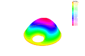
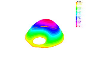
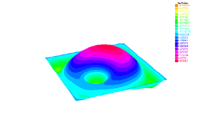
Figure 1: Example 1. The solution of the elliptic problem (1.2)-(1.3) in the domain $\Omega_{g}$ (left), in the domain bounded by the zero level sets of $y_{\epsilon}$ (right) and the final computed state $y_{\epsilon}$ in $D$ (bottom).

If $r_{h},\ v_{h}$ are given by Proposition 4.4 and $\gamma>0$ is a scaling parameter, then $\gamma r_{h}$ and $v_{h}$ verify (4.45), that is they also give a descent direction. We take the scaling parameter for $r_{h}$ given by $\gamma=\frac{1}{\max(r_{h})}$, that is a normalization of $r_{h}$. In this way we avoid the appearance of very high values of the objective function, that may stop the algorithm even in the first iteration. For the line search at the Step 4, we use $\lambda=\rho^{i}\lambda_{0}$, with $\lambda_{0}=1$, $\rho=0.5$ for $i=0,1,\dots,30$.

The stopping test is obtained for $k=94$ and some values of the objective function are: $J(G^{0},U^{0})=33110.5$, $J(G^{30},U^{30})=54.725$, $J(G^{94},U^{94})=14.9851$.

At the final iteration, the first term of the optimal objective function is $1.03796$ and $\int_{\partial\Omega_{g}}y_{\epsilon}^{2}(s)ds=1.39471\times 10^{-2}$. We point out that the optimal $\Omega_{g}$ has a hole and the penalization term is a sum of two integrals

$$\int_{\partial\Omega_{g}}y_{\epsilon}^{2}(s)ds=\sum_{j=1}^{2}\int_{I_{j}}\left(y_{\epsilon}(\mathbf{z}_{g}(t))\right)^{2}|\mathbf{z}_{g}^{\prime}(t)|dt$$

where the integral over $I_{1}$ corresponding to the exterior boundary of $\Omega_{g}$ and $I_{2}$ to the boundary of the hole. In Figure 1 in the bottom, we can see the computed optimal state $y_{\epsilon}$ in iteration 94. We also compute the costs $\int_{E}(y_{1}-y_{d})^{2}d\mathbf{x}=0.998189$ where $y_{1}$ is the solution of the initial elliptic problem (1.2)-(1.3) in the domain $\Omega_{g}$ with g obtained in iteration 94 and $\int_{E}(y_{2}-y_{d})^{2}d\mathbf{x}=1.04032$ where $y_{2}$ is the solution of the elliptic problem (1.2)-(1.3) in the domain bounded by the zero level sets of $y_{\epsilon}$ in iteration 94, see Figure 1.

Example 2.

The domains $D$, $E$ and the mesh of $D$ are the same as in Example 1. For $f=4$ and $y_{d}(x_{1},x_{2})=-x_{1}^{2}-x_{2}^{2}+1$, we have the exact optimal state $y=y_{d}$ defined in the disk of center $(0,0)$ and radius $1$, that gives an optimal domain of the problem (1.1)-(1.3).

We have used $\epsilon=10^{-1}$ and the starting configuration: the disk of center $(0,0)$ and radius $2.5$ with the circular hole of center $(-1,-1)$ and radius $0.5$. We use $(R^{k},V^{k})$ given by Proposition 4.4. The parameters for the line search and $\gamma$ are the same as in the precedent example.

The stopping test is obtained for $k=64$. The initial and the final computed values of the objective function are $5368.84$ and $11.2311$. We obtain a local minimum that is different from the above global solution. The first term of the final computed objective function is $0.472856$. The term $\int_{\partial\Omega_{g}}y_{\epsilon}^{2}(s)ds$ is $1.07583$ and it was computed over the exterior boundary as well as over the boundaries of two holes. The length of the total boundary of the optimal domain is $23.9714$ and of the initial domain is $2\pi(2.5+0.5)=18.8495$.

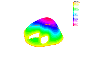
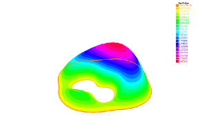
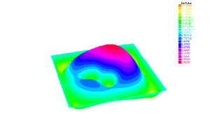
Figure 2: Example 2. The numerical solution of the elliptic problem (1.2)-(1.3) in the optimal domain $\Omega_{g}$ (left), in the domain bounded by the zero level sets of $y_{\epsilon}$ (right) and the computed optimal state $y_{\epsilon}$ (bottom).

The domain changes its topology. The computed optimal state $y_{\epsilon}$ is presented in Figure 2 in the bottom. At the left, we show $y_{1}$ the solution of the elliptic problem (1.2)-(1.3) in the domain $\Omega_{g}$ which gives $\int_{E}(y_{1}-y_{d})^{2}d\mathbf{x}=0.295178$, at the right we show $y_{2}$ the solution of the elliptic problem (1.2)-(1.3) in the domain bounded by the zero level sets of $y_{\epsilon}$, which gives $\int_{E}(y_{2}-y_{d})^{2}d\mathbf{x}=0.471788$.

Example 3.

We have also used the descent direction given by Proposition 4.5, for the starting configuration the disk of center $(0,0)$ and radius $1.5$, $\epsilon=10^{-1}$, $\gamma=\frac{1}{\|r_{h}\|_{\infty}}$ and a mesh of $D$ of 32446 triangles and 16464 vertices. For solving the ODE systems (4.3)-(4.5) and (4.2)-(4.13) we use $m=30$.

At the initial iteration, we have $\int_{E}(y_{\epsilon}-y_{d})^{2}d\mathbf{x}=72.3767$, $\int_{\partial\Omega_{g}}y_{\epsilon}^{2}(s)ds=658.459$ and the value of the objective function is $J_{0}=6656.98$. The algorithm stops after 12 iterations and we have at the final iteration $\int_{E}(y_{\epsilon}-y_{d})^{2}d\mathbf{x}=1.22861$, $\int_{\partial\Omega_{g}}y_{\epsilon}^{2}(s)ds=0.557556$ and the value of the penalized objective function is $J_{12}=6.80521$. The final domain is a perturbation of the initial one, the circular non-smooth curve in the top, left image of Figure 3. We have $\int_{E}(y_{1}-y_{d})^{2}d\mathbf{x}=1.20398$ for $y_{1}$ the solution of the elliptic problem (1.2)-(1.3) in the final domain $\Omega_{g}$ and $\int_{E}(y_{2}-y_{d})^{2}d\mathbf{x}=1.21767$ for $y_{2}$ the solution of the elliptic problem (1.2)-(1.3) in the domain bounded by the zero level sets of $y_{\epsilon}$, Figure 3 at the bottom, right.

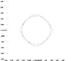
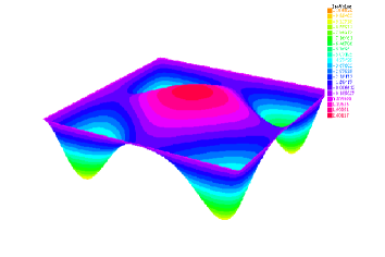
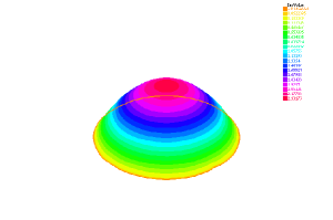
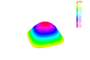
Figure 3: Example 3. The zero level sets of the computed optimal $g$, $y_{\epsilon}$ (top, left), the final state $y_{\epsilon}$ (top, right), the solution of the elliptic problem (1.2)-(1.3) in the domain $\Omega_{g}$ (bottom, left) and in the domain bounded by the zero level sets of $y_{\epsilon}$ (bottom, right).

Finally, we notice that the hypothesis of Proposition 3.3 is obviously fulfilled by the null level sets of $y_{\epsilon}$ with a corresponding parametrization. In an approximate sense, it is also fulfilled by the computed optimal domain $\Omega_{g}$ since the penalization integral is ”small” in all the examples.

References

- [1] E. G. Allaire, Shape optimization by the homogenization method. Springer, New York, 2002.
- [2] V. Barbu and Th. Precupanu, Convexity and optimization in Banach spaces. Mathematics and its Applications, 10. D. Reidel Publishing Co., Dordrecht; Editura Academiei, Bucharest, 1986.
- [3] M. Bendsoe and O. Sigmund, Topology Optimization: Theory, Methods and Applications. 2-nd edition, Engineering online library, Springer, Berlin, 2003.
- [4] F. Bouchut and L. Desvillets, On two-dimensional Hamiltonian transport equations with continuous coefficients. Differential and Integral Equations, 14 (2001) 1015–1024, N. 8, https://projecteuclid.org/euclid.die/1356123178.
- [5] D. Bucur and G. Buttazzo, Variational methods in shape optimization problems. Progress in Nonlinear Differential Equations and their Applications, 65. Birkhauser Boston, Inc., Boston, MA, 2005.
- [6] P. G. Ciarlet, The finite element method for elliptic problems. Classics in Applied Mathematics, 40. Society for Industrial and Applied Mathematics (SIAM), Philadelphia, PA, 2002.
- [7] F. H. Clarke, Optimization and nonsmooth analysis. Canadian Mathematical Society Series of Monographs and Advanced Texts. A Wiley-Interscience Publication. John Wiley & Sons, Inc., New York, 1983.
- [8] M. C. Delfour and J. P. Zolesio, Shapes and Geometries, Analysis, Differential Calculus and Optimization, SIAM, Philadelphia, 2001.
- [9] F. Hecht, New development in FreeFem++. J. Numer. Math. 20 (2012) 251–265. http://www.freefem.org
- [10] A. Henrot and M. Pierre, Variations et optimisation de formes. Une analyse géométrique, Springer, 2005.
- [11] M.W. Hirsch, S. Smale and R.L. Devaney, Differential equations, dynamical systems and an introduction to chaos., Elsevier, Academic Press, San Diego, 2004.
- [12] J.-L. Lions, Quelques méthodes de résolution des problèmes aux limites non linéaires. Dunod; Gauthier-Villars, Paris 1969.
- [13] R. Mäkinen, P. Neittaanmäki and D. Tiba, On a fixed domain approach for a shape optimization problem. In: W. F. Ames, P. J. van der Houwen (Eds), Computational and Applied Mathematics II: Differential Equations, North-Holland, Amsterdam, 1992, pp. 317–326.
- [14] P. Neittaanmäki, A. Pennanen and D. Tiba, Fixed domain approaches in shape optimization problems with Dirichlet boundary conditions, Inverse Problems 25 (2009) 1–18.
- [15] P. Neittaanmäki, J. Sprekels and D. Tiba, Optimization of elliptic systems. Theory and applications, Springer, New York, 2006.
- [16] P. Neittaanmäki and D. Tiba, Optimal control of nonlinear parabolic systems. Theory, algorithms, and applications. Monographs and Textbooks in Pure and Applied Mathematics, 179. Marcel Dekker, Inc., New York, 1994.
- [17] P. Neittaanmäki and D. Tiba, Fixed domain approaches in shape optimization problems, Inverse Problems 28 (2012) 1–35.
- [18] M. R. Nicolai and D. Tiba, Implicit functions and parametrizations in dimension three: generalized solutions. Discrete Contin. Dyn. Syst. 35 (2015), no. 6, 2701–2710.
- [19] S. Osher and J. Sethian, Fronts propagating with curvature-dependent speed. Journal of Computational Physics, 79 (1988) 12–49.
- [20] O. Pironneau, Optimal shape design for elliptic systems, Springer, Berlin, 1984.
- [21] P.-A. Raviart and J.-M. Thomas, Introduction à l’analyse numérique des équations aux dérivées partielles. Dunod, 2004.
- [22] T.C. Sideris, Ordinary differential equations and dynamical systems, Atlantis Press, Paris, 2013.
- [23] J. Sokolowski and J.P. Zolesio, Introduction to Shape Optimization. Shape Sensitivity Analysis, Springer, Berlin, 1992.
- [24] D. Tiba, The implicit function theorem and implicit parametrizations. Ann. Acad. Rom. Sci. Ser. Math. Appl. 5 (2013), no. 1–2, 193–208.
- [25] D. Tiba, Iterated Hamiltonian type systems and applications. J. Differential Equations 264 (2018), no. 8, 5465–5479.
- [26] D. Tiba, A penalization approach in shape optimization, Atti della Accad. Pelorit. Pericol. - Cl. Sci. Fis., Mat. Nat., 96 No.1, A8 (2018) DOI: 10.1478/AAPP.961A8.