Fully Discrete Positivity-Preserving and Energy-Dissipating Schemes for Aggregation-Diffusion Equations with a Gradient-Flow Structure

Abstract

We propose fully discrete, implicit-in-time finite-volume schemes for a general family of non-linear and non-local Fokker-Planck equations with a gradient-flow structure, usually known as aggregation-diffusion equations, in any dimension. The schemes enjoy the positivity-preservation and energy-dissipation properties, essential for their practical use. The first-order scheme verifies these properties unconditionally for general non-linear diffusions and interaction potentials, while the second-order scheme does so provided a CFL condition holds. Sweeping dimensional splitting permits the efficient construction of these schemes in higher dimensions while preserving their structural properties. Numerical experiments validate the schemes and show their ability to handle complicated phenomena typical in aggregation-diffusion equations, such as free boundaries, metastability, merging and phase transitions.

AMS Subject Classification — 35Q70; 35Q91; 45K05; 65M08.

Keywords — Gradient flows; finite-volume methods; fully discrete schemes; positivity preservation; energy dissipation; integro-differential equations.

1 Introduction

This work concerns the family of non-linear and non-local aggregation-diffusion equations

$$\left\{\begin{aligned} &\partial_{t}\rho=\nabla\cdot[\rho\nabla(H^{\prime}(\rho)+V+W\ast\rho)],\quad\mathbf{x}\in{\mathbb{R}^{d}},\ t>0,\\ &\rho(0,\mathbf{x})=\rho_{0}(\mathbf{x}),\end{aligned}\right.$$ (1.1)

where $\rho=\rho(t,\mathbf{x})\geq 0$ is the unknown particle density, $H(\rho)$ is the density of internal energy, $V(\mathbf{x})$ is the confinement potential, and $W(\mathbf{x})$ is the so-called interaction potential; see [34, 63]. $H$ is a convex function by definition, in order to ensure that the first term, $\nabla\cdot[\rho H^{\prime\prime}(\rho)\nabla\rho]$, is a (possibly degenerate) non-linear density-dependent diffusion. The drift terms $\nabla\cdot[\rho\nabla V]$ and $\nabla\cdot[\rho\nabla(W\ast\rho)]$ correspond respectively to forces acting on the particles due to external sources $V(\mathbf{x})$, and to attractive-repulsive forces between particles given by a potential $W(\mathbf{x})$.

These equations can be derived as mean-field limits of particle systems or as upscalings of cellular automata, and have applications in granular materials [7, 8, 6], cell migration and chemotaxis [15, 18, 49, 25], collective motion of animals (swarming) [59, 48, 30], opinion formation [51, 43], self-assembly of nanoparticles [46], and mathematical finance [42], among others. In the case of linear diffusion, these models correspond to macroscopic limits of interacting particle systems in terms of Fokker-Planck type equations; see, for instance, [58, 12] and the references therein. They can lead to interesting evolutionary phenomena, such as noise-induced phase transitions or metastability behaviour [4, 44, 5], present too in non-linear diffusion models [17, 22, 25]. Typical interaction potentials $W(\mathbf{x})$ which appear in applications are radial, and can be fully attractive, such as the Newtonian and Bessel potentials in chemotaxis [25] or power-laws in granular materials [34]; repulsive in the short range and attractive in the long range, such as combinations of power-law or Morse-type potentials in swarming [59, 33]; or compactly supported potentials in many biological applications, such as networks and cell sorting [5, 23].

Equation 1.1 possesses interesting properties. First, its solution is always a non-negative density. Second, it has a variational structure: it is the gradient flow of a free energy, as discovered in [34]. We can define the free-energy functional by

$$E(\rho)=\int_{{\mathbb{R}^{d}}}[H(\rho)+V\rho+\frac{1}{2}(W\ast\rho)\rho]\,\mathop{}\!\mathrm{d}{\mathbf{x}}\,,$$ (1.2)

whose formal variation for zero mass perturbations is given by $\xi:=\frac{\delta E}{\delta\rho}=H^{\prime}(\rho)+V+W\ast\rho$; the evolution of the free energy along a solution of (1.1) is given by

$$\frac{\mathop{}\!\mathrm{d}{E}}{\mathop{}\!\mathrm{d}{t}}=\int_{{\mathbb{R}^{d}}}\frac{\delta E}{\delta\rho}\frac{\partial\rho}{\partial t}\,\mathop{}\!\mathrm{d}{\mathbf{x}}=\int_{{\mathbb{R}^{d}}}\xi\nabla\cdot[\rho\nabla\xi]\,\mathop{}\!\mathrm{d}{\mathbf{x}}=-\int_{{\mathbb{R}^{d}}}\rho|\nabla\xi|^{2}\,\mathop{}\!\mathrm{d}{\mathbf{x}}\leq 0.$$ (1.3)

This dissipation property has another interpretation: the solution to (1.1) is the gradient flow or the curve of steepest descent for the free energy functional $E$ in the sense of the Euclidean transport distance between probability measures, as discussed in [2, 34, 25] and the references therein. We remark that these structural properties persist when the equation is solved in a bounded domain $\Omega$ with no-flux boundary conditions, provided the convolution is understood by extending the density as zero outside $\Omega$, and that $\nabla\xi\cdot\eta(x)=0$ is satisfied for all $x\in\partial\Omega$, where $\eta(x)$ is the outwards unit normal vector to the boundary of $\Omega$.

It is important to notice that the dissipation property entails a full characterisation of the set of stationary states: they are given by non-negative densities such that $\xi$ is constant (possibly different) in each connected component of their support. Therefore, the free energy is a Lyapunov functional for (1.1), and will be useful to discuss the stability of the equilibria in many particular cases, see [34, 32].

These non-linear Fokker-Planck equations have drawn much attention by the numerical analysis and simulation communities in recent times. Indeed, a central question has been the design of numerical schemes capable of preserving the structural properties of the gradient flow (1.1): the non-negativity of the solution, the dissipation property (1.3), and a corresponding discrete set of stationary states which accurately capture the long-time asymptotics of these equations. First and second-order-accurate finite-volume schemes which treat Eq. 1.1 as a non-linear continuity equation (with a vector field given by $-\nabla\xi$) were proposed in [9] for non-linear diffusions, and in [22] for aggregation-diffusion equations. Their explicit discretisations preserve the positivity-preservation property under a CFL condition; entropy dissipation is shown for the semi-discrete schemes (continuous in time). A generalisation of these ideas for high-order approximations has been proposed in [57], using a discontinuous Galerkin approach with a suitable quadrature rule which employs Gauss-Lobatto formulas.

In the case of linear diffusion, schemes which enjoy the semi-discrete energy-dissipation property were known for Fokker-Planck equations in granular media [13, 14], based on the Chang-Cooper discretisation approach [37]. Such schemes have been generalised and improved for equations of the form (1.1) in [52], leading to second-order-accurate finite-difference schemes, again with a semi-discrete dissipation. Linear Fokker-Planck equations have many other entropies; for instance, spectral schemes were used in [45] to achieve the dissipation of the weighted $L^{2}$ entropies. Finally, implicit-in-time semi-discretisations were proposed in [3, 31] which dissipate the discrete-in-time energy for non-linear Fokker-Planck equations corresponding to (1.1) with $W=0$. These schemes are reminiscent of the convex splitting ideas in the variational $L^{2}$ framework, as developed in [55]; however, they are not directly applicable in the setting of gradient flows with respect to measures. Other numerical schemes used for non-linear Fokker-Planck equations include finite-element schemes [16]; particle/blob methods [40, 19, 24]; and approaches based on the gradient flow formulation, in terms of the steepest descent of Euclidean transport distances [11, 35, 50, 47, 36, 29].

In a recent work [1], several fully discrete, implicit-in-time discretisations have been proposed for the Keller-Segel model in one dimension (with linear diffusion and non-linear chemosensitivity) which possess the energy dissipation property. Among them, they presented an implicit-in-time, fully discrete scheme based on the gradient flow ideas of [17, 22, 57]. In the present work we generalise these ideas proposing fully discrete (in both space and time), implicit finite-volume schemes for Equation 1.1 which are both positivity-preserving and energy-dissipating; these properties are met unconditionally by a scheme with first-order accuracy in time and space, and met under a parabolic CFL condition by a second-order-in-space scheme. Both schemes work for general non-linear diffusions and general interaction potentials $W$, through a careful combination of the implicit-in-time discretisations as hinted in [1]. Special care has to be taken in using the implicit schemes as the Jacobian matrix can be ill-conditioned in the presence of vacuum, due to the non-linear diffusion terms. A detailed study of the positivity for these schemes is done via M-matrix arguments.

Our next contribution is to propose for the first time a combination of these gradient-flow schemes with a generalised dimensional splitting technique; this results in fully discrete, implicit finite-volume schemes for Eq. 1.1, which are positivity-preserving and energy-dissipating in higher dimensions with a reasonable computational cost. We remark that a direct generalisation of the one-dimensional schemes presented here and in [1] to multiple dimensions is possible, but comes with a very high computational cost caused by the inversion of large Jacobian matrices. Our approach takes advantage of the dimensional splitting to drastically reduce this cost without sacrificing the fundamental properties of the scheme.

The rest of this work is organised as follows: Section 2 will discuss the time discretisation for (1.1) in a way that preserves the energy dissipation for general non-linearities and interaction potentials; Section 3 is devoted to the fully discrete scheme in the one-dimensional setting; Sections 4 and 5 respectively introduce the dimensional splitting and the sweeping dimensional splitting formulations for higher dimensions; Section 6 is aimed at validating the numerical scheme on explicit solutions for both non-linear diffusions and aggregations; finally, Section 7 presents numerical experiments that showcase the effectiveness of the new scheme in dealing with complicated phenomena, such as metastability or phase transitions, both in one and two dimensions, with linear and non-linear diffusions.

2 Time Discretisation

The choice of time discretisation is an integral step in the construction a fully discrete, energy-dissipating scheme. In this section, we shall consider two discretisations, which will lead to two fully discrete schemes, discussed later in the work.

To begin, we define the semi-discrete energy at time $t^{n}$ as follows:

$$E(\rho^{n})=\int_{{\mathbb{R}^{d}}}H(\rho^{n})+V\rho^{n}+\frac{1}{2}(W\ast\rho^{n})\rho^{n}\,\mathop{}\!\mathrm{d}{\mathbf{x}}.$$ (2.1)

For the sake of generality, consider the following first-order scheme:

$$\frac{\rho^{n+1}-\rho^{n}}{\Delta t}=\nabla\cdot(\rho^{*}\nabla(H^{\prime}(\rho^{n+1})+V+W\ast\rho^{**})),$$ (2.2)

where $\rho^{*}$ and $\rho^{**}$ can be either $\rho^{n}$ or $\rho^{n+1}$ and will be specified later. Here, we have chosen $H^{\prime}(\rho^{n+1})$ over $H^{\prime}(\rho^{n})$ because the explicit case has been explored in [3, 31] and does not lead to a fully discrete dissipation of the free energy. We now attempt to show that scheme (2.2) verifies $E(\rho^{n+1})\leq E(\rho^{n})$, provided $\rho^{n}\geq 0$, at any time step $t^{n}$. To this end, we first multiply both sides of (2.2) by $H^{\prime}(\rho^{n+1})+V+W\ast\rho^{**}$ and integrate to obtain

$$\int_{{\mathbb{R}^{d}}}(\rho^{n+1}-\rho^{n})(H^{\prime}(\rho^{n+1})+V+W\ast\rho^{**})\,\mathop{}\!\mathrm{d}{\mathbf{x}}$$ (2.3)

$$=-\Delta t\int_{{\mathbb{R}^{d}}}\rho^{*}|\nabla(H^{\prime}(\rho^{n+1})+V+W\ast\rho^{**})|^{2}\,\mathop{}\!\mathrm{d}{\mathbf{x}},$$ (2.4)

using integration by parts on the right-hand side. From (2.4), we have

$$\int_{{\mathbb{R}^{d}}}(\rho^{n+1}-\rho^{n})V\,\mathop{}\!\mathrm{d}{\mathbf{x}} =-\int_{{\mathbb{R}^{d}}}(\rho^{n+1}-\rho^{n})(H^{\prime}(\rho^{n+1})+W\ast\rho^{**})\,\mathop{}\!\mathrm{d}{\mathbf{x}}$$ (2.5)

$$\quad-\Delta t\int_{{\mathbb{R}^{d}}}\rho^{*}|\nabla(H^{\prime}(\rho^{n+1})+V+W\ast\rho^{**})|^{2}\,\mathop{}\!\mathrm{d}{\mathbf{x}}.$$ (2.6)

Then,

$$E(\rho^{n+1})-E(\rho^{n})$$ (2.7)

$$=\int_{{\mathbb{R}^{d}}}H(\rho^{n+1})-H(\rho^{n})+(\rho^{n+1}-\rho^{n})V+\frac{1}{2}(W\ast\rho^{n+1})\rho^{n+1}-\frac{1}{2}(W\ast\rho^{n})\rho^{n}\,\mathop{}\!\mathrm{d}{\mathbf{x}}$$ (2.8)

$$=\int_{{\mathbb{R}^{d}}}H(\rho^{n+1})-H(\rho^{n})-(\rho^{n+1}-\rho^{n})H^{\prime}(\rho^{n+1})\,\mathop{}\!\mathrm{d}{\mathbf{x}}$$ (2.9)

$$\quad+\int_{{\mathbb{R}^{d}}}\frac{1}{2}(W\ast\rho^{n+1})\rho^{n+1}-\frac{1}{2}(W\ast\rho^{n})\rho^{n}-(\rho^{n+1}-\rho^{n})(W\ast\rho^{**})\,\mathop{}\!\mathrm{d}{\mathbf{x}}$$ (2.10)

$$\quad-\Delta t\int_{{\mathbb{R}^{d}}}\rho^{*}|\nabla(H^{\prime}(\rho^{n+1})+V+W\ast\rho^{**})|^{2}\,\mathop{}\!\mathrm{d}{\mathbf{x}}$$ (2.11)

$$=I+II+III,$$ (2.12)

having used (2.6) in the second equality. Here,

$$I :=\int_{{\mathbb{R}^{d}}}H(\rho^{n+1})-H(\rho^{n})-(\rho^{n+1}-\rho^{n})H^{\prime}(\rho^{n+1})\,\mathop{}\!\mathrm{d}{\mathbf{x}};$$ (2.13)

$$II :=\int_{{\mathbb{R}^{d}}}\frac{1}{2}(W\ast\rho^{n+1})\rho^{n+1}-\frac{1}{2}(W\ast\rho^{n})\rho^{n}-(\rho^{n+1}-\rho^{n})(W\ast\rho^{**})\,\mathop{}\!\mathrm{d}{\mathbf{x}};$$ (2.14)

$$III :=-\Delta t\int_{{\mathbb{R}^{d}}}\rho^{*}|\nabla(H^{\prime}(\rho^{n+1})+V+W\ast\rho^{**})|^{2}\,\mathop{}\!\mathrm{d}{\mathbf{x}}.$$ (2.15)

Our goal is to show that $I+II+III\leq 0$ in order to arrive at $E(\rho^{n+1})\leq E(\rho^{n})$. In part $I$,

$$H(\rho^{n+1})-H(\rho^{n})\leq(\rho^{n+1}-\rho^{n})H^{\prime}(\rho^{n+1}),$$ (2.16)

which follows from the convexity of $H$; hence, $I\leq 0$, as already pointed out in [3, 31].

In part $II$, there are several possible choices for $\rho^{**}$, explored below.

Explicit Case.

If $\rho^{**}=\rho^{n}$, we have

$$II(\rho^{n}) :=\int_{{\mathbb{R}^{d}}}\frac{1}{2}(W\ast\rho^{n+1})\rho^{n+1}-\frac{1}{2}(W\ast\rho^{n})\rho^{n}-(\rho^{n+1}-\rho^{n})(W\ast\rho^{n})\,\mathop{}\!\mathrm{d}{\mathbf{x}}$$

$$=\frac{1}{2}\int_{{\mathbb{R}^{d}}}\left[(W\ast\rho^{n+1})\rho^{n+1}-2(W\ast\rho^{n})\rho^{n+1}+(W\ast\rho^{n})\rho^{n}\right]\,\mathop{}\!\mathrm{d}{\mathbf{x}}$$

$$=\frac{1}{2}\iint_{\mathbb{R}^{2d}}W(\mathbf{x}-\mathbf{y})(\rho^{n+1}(\mathbf{x})-\rho^{n}(\mathbf{x}))(\rho^{n+1}(\mathbf{y})-\rho^{n}(\mathbf{y}))\,\mathop{}\!\mathrm{d}{\mathbf{x}}\mathop{}\!\mathrm{d}{\mathbf{y}},$$ (2.17)

since $W$ is symmetric. If $W(\mathbf{x})=\frac{|\mathbf{x}|^{2}}{2}$:

$$II(\rho^{n}) =\frac{1}{2}\iint_{\mathbb{R}^{2d}}\left(\frac{|\mathbf{x}|^{2}}{2}-\mathbf{x}\cdot\mathbf{y}+\frac{|\mathbf{y}|^{2}}{2}\right)(\rho^{n+1}(\mathbf{x})-\rho^{n}(\mathbf{x}))(\rho^{n+1}(\mathbf{y})-\rho^{n}(\mathbf{y}))\,\mathop{}\!\mathrm{d}{\mathbf{x}}\mathop{}\!\mathrm{d}{\mathbf{y}}$$ (2.18)

$$=\frac{1}{2}\left[\left(\int_{{\mathbb{R}^{d}}}\frac{|\mathbf{x}|^{2}}{2}(\rho^{n+1}(\mathbf{x})-\rho^{n}(\mathbf{x}))\,\mathop{}\!\mathrm{d}{\mathbf{x}}\right)\left(\int_{{\mathbb{R}^{d}}}\rho^{n+1}(\mathbf{y})-\rho^{n}(\mathbf{y})\,\mathop{}\!\mathrm{d}{\mathbf{y}}\right)\right.$$ (2.19)

$$\quad+\left(\int_{{\mathbb{R}^{d}}}\frac{|\mathbf{y}|^{2}}{2}(\rho^{n+1}(\mathbf{y})-\rho^{n}(\mathbf{y}))\,\mathop{}\!\mathrm{d}{\mathbf{y}}\right)\left(\int_{{\mathbb{R}^{d}}}\rho^{n+1}(\mathbf{x})-\rho^{n}(\mathbf{x})\,\mathop{}\!\mathrm{d}{\mathbf{x}}\right)$$ (2.20)

$$\quad\left.-\left(\int_{{\mathbb{R}^{d}}}\mathbf{x}(\rho^{n+1}(\mathbf{x})-\rho^{n}(\mathbf{x}))\,\mathop{}\!\mathrm{d}{\mathbf{x}}\right)\cdot\left(\int_{{\mathbb{R}^{d}}}\mathbf{y}(\rho^{n+1}(\mathbf{y})-\rho^{n}(\mathbf{y}))\,\mathop{}\!\mathrm{d}{\mathbf{y}}\right)\right]$$ (2.21)

$$=-\frac{1}{2}\left|\int_{{\mathbb{R}^{d}}}\mathbf{x}(\rho^{n+1}(\mathbf{x})-\rho^{n}(\mathbf{x}))\,\mathop{}\!\mathrm{d}{\mathbf{x}}\right|^{2}\leq 0,$$ (2.22)

where we used the conservation of mass property,

$$\int_{{\mathbb{R}^{d}}}\rho^{n+1}(\mathbf{x})\,\mathop{}\!\mathrm{d}{\mathbf{x}}=\int_{{\mathbb{R}^{d}}}\rho^{n}(\mathbf{x})\,\mathop{}\!\mathrm{d}{\mathbf{x}}.$$ (2.23)

If $\hat{W}(\xi)\leq 0$, where $\hat{W}(\xi)$ is the Fourier transform of $W(\mathbf{x})$:

$$II(\rho^{n}) =\frac{1}{2}\int_{{\mathbb{R}^{d}}}(W\ast(\rho^{n+1}-\rho^{n}))(\mathbf{x})(\rho^{n+1}(\mathbf{x})-\rho^{n}(\mathbf{x}))\,\mathop{}\!\mathrm{d}{\mathbf{x}},$$ (2.24)

$$=\frac{1}{2}\iint_{\mathbb{R}^{2d}}\hat{W}(\xi)(\hat{\rho}^{n+1}(\xi)-\hat{\rho}^{n}(\xi))(\rho^{n+1}(\mathbf{x})-\rho^{n}(\mathbf{x}))e^{2\pi i\mathbf{x}\cdot\xi}\,\mathop{}\!\mathrm{d}{\xi}\,\mathop{}\!\mathrm{d}{\mathbf{x}},$$

$$=\frac{1}{2}\int_{\mathbb{R}^{d}}\hat{W}(\xi)(\hat{\rho}^{n+1}(\xi)-\hat{\rho}^{n}(\xi))(\hat{\rho}^{n+1}(-\xi)-\hat{\rho}^{n}(-\xi))\,\mathop{}\!\mathrm{d}{\xi},$$

$$=\frac{1}{2}\int_{\mathbb{R}^{d}}\hat{W}(\xi)(\hat{\rho}^{n+1}(\xi)-\hat{\rho}^{n}(\xi))(\overline{\hat{\rho}^{n+1}(\xi)}-\overline{\hat{\rho}^{n}(\xi)})\,\mathop{}\!\mathrm{d}{\xi},$$

$$=\frac{1}{2}\int_{{\mathbb{R}^{d}}}\hat{W}(\xi)|\hat{\rho}^{n+1}(\xi)-\hat{\rho}^{n}(\xi)|^{2}\,\mathop{}\!\mathrm{d}{\xi}\leq 0.$$

Implicit Case.

If $\rho^{**}=\rho^{n+1}$, we have

$$II(\rho^{n+1}) :=\int_{{\mathbb{R}^{d}}}\frac{1}{2}(W\ast\rho^{n+1})\rho^{n+1}-\frac{1}{2}(W\ast\rho^{n})\rho^{n}-(\rho^{n+1}-\rho^{n})(W\ast\rho^{n+1})\,\mathop{}\!\mathrm{d}{\mathbf{x}},$$

$$=-\frac{1}{2}\int_{{\mathbb{R}^{d}}}\left[(W\ast\rho^{n+1})\rho^{n+1}-2(W\ast\rho^{n})\rho^{n+1}+(W\ast\rho^{n})\rho^{n}\right]\,\mathop{}\!\mathrm{d}{\mathbf{x}},$$

$$=-\frac{1}{2}\iint_{\mathbb{R}^{2d}}W(\mathbf{x}-\mathbf{y})(\rho^{n+1}(\mathbf{x})-\rho^{n}(\mathbf{x}))(\rho^{n+1}(\mathbf{y})-\rho^{n}(\mathbf{y}))\,\mathop{}\!\mathrm{d}{\mathbf{x}}\mathop{}\!\mathrm{d}{\mathbf{y}}=-II(\rho^{n}),$$ (2.25)

which is just the negative of the previous case. Thus, we conclude $II(\rho^{n+1})\leq 0$ for $W(\mathbf{x})=-\frac{|\mathbf{x}|^{2}}{2}$ and $\hat{W}(\xi)\geq 0$.

Unconditional Case.

If $\rho^{**}=(\rho^{n+1}+\rho^{n})/{2}$, we have

$$II=\int_{{\mathbb{R}^{d}}}\frac{1}{2}(W\ast\rho^{n+1})\rho^{n+1}-\frac{1}{2}(W\ast\rho^{n})\rho^{n}-\frac{1}{2}(\rho^{n+1}-\rho^{n})(W\ast(\rho^{n+1}+\rho^{n}))\,\mathop{}\!\mathrm{d}{\mathbf{x}}=0.$$

Therefore, $II$ is exactly zero regardless of the choice of $W$.

Finally, $III\leq 0$ follows from the positivity of $\rho^{*}$, chosen as either $\rho^{n}$ or $\rho^{n+1}$. We now remark that the computations above remain unaltered when considered over a bounded domain $\Omega$ with no-flux boundary conditions. It is a simple exercise to check that the boundary terms left by the integration by parts vanish.

Henceforth, an interaction $W$ satisfying $II(\rho^{n})=-II(\rho^{n+1})\leq 0$ (respectively $II(\rho^{n})=-II(\rho^{n+1})\geq 0$) will be referred as a negative-definite (resp. positive-definite) interaction potential. We have just shown that attractive (resp. repulsive) quadratic potentials, as well as certain catastrophic (resp. H-stable) potentials (according to the notation of classical statistical mechanics in [54]), are negative definite (resp. positive definite). These potentials are very relevant in applications for the existence of both steady states and phase transitions, with and without (linear or non-linear) diffusion terms; see [20, 26, 27, 38, 5, 32] and the references therein.

To summarise, a suitable choice of $\rho^{**}$, given $W$, always exists, and we have obtained two time discretisation methods which satisfy an energy dissipation property:

Proposition 2.1.

1. The implicit time discretisation

   $$\frac{\rho^{n+1}-\rho^{n}}{\Delta t}=\nabla\cdot(\rho^{n}\nabla(H^{\prime}(\rho^{n+1})+V+W\ast\rho^{**})),$$ (2.26)

   satisfies the energy dissipation property, i.e., $E(\rho^{n+1})\leq E(\rho^{n})$, if one of the following conditions holds:

   1. $\rho^{**}=(\rho^{n+1}+\rho^{n})/{2}$;

   2. $\rho^{**}=\rho^{n}$ and $W$ is a negative-definite interaction potential;

   3. $\rho^{**}=\rho^{n+1}$ and $W$ is a positive-definite interaction potential.

2. The implicit time discretisation

   $$\frac{\rho^{n+1}-\rho^{n}}{\Delta t}=\nabla\cdot(\rho^{n+1}\nabla(H^{\prime}(\rho^{n+1})+V+W\ast\rho^{**})),$$ (2.27)

   satisfies the energy dissipation property, i.e., $E(\rho^{n+1})\leq E(\rho^{n})$, if one of the following conditions holds:

   1. $\rho^{**}=(\rho^{n+1}+\rho^{n})/{2}$;

   2. $\rho^{**}=\rho^{n}$ and $W$ is a negative-definite interaction potential;

   3. $\rho^{**}=\rho^{n+1}$ and $W$ is a positive-definite interaction potential.

It is an interesting open problem to show that the schemes (2.26) and (2.27) are well posed in the set of non-negative densities, for small enough $\Delta t$, under reasonable assumptions on the potentials.

3 Fully Discrete Schemes in One Dimension

In this section we present fully discrete schemes in one dimension, by coupling the time discretisations of Section 2 with the finite-volume method in space. We introduce two schemes, corresponding to the discretisations (2.26) and (2.27).

To begin, we consider a large computational domain $\Omega=[-L,L]$, for $L>0$, and divide it into $2M$ uniform cells of size $\Delta x=L/M$. We denote the $i$-th cell by $C_{i}=[x_{i-1/2},x_{i+1/2}]$ for $i=1,\dots,2M$; the cell centre is $x_{i}=-L+\Delta x(i-1/2)$. No-flux boundary conditions are assumed at the boundaries.

3.1 Scheme 1 (S1)

This scheme is based on the implicit time discretisation (2.26). The spatial discretisation follows the fully explicit finite-volume method in [22], where only semi-discrete energy dissipation was shown (continuous in time). By modifying certain terms into implicit form, we obtain a fully discrete, energy-dissipating scheme with second-order accuracy in space.

Assume $\rho_{i}$ is the cell average on $C_{i}$; the scheme reads

$$\begin{split}&\frac{\rho_{i}^{n+1}-\rho_{i}^{n}}{\Delta t}+\frac{F_{i+1/2}^{n+1}-F_{i-1/2}^{n+1}}{\Delta x}=0,\\ &F_{i+1/2}^{n+1}=\rho_{i}^{E}(u_{i+1/2}^{n+1})^{+}+\rho_{i+1}^{W}(u_{i+1/2}^{n+1})^{-},\\ &(u_{i+1/2}^{n+1})^{+}=\max(u_{i+1/2}^{n+1},0),\qquad(u_{i+1/2}^{n+1})^{-}=\min(u_{i+1/2}^{n+1},0),\\ &u_{i+1/2}^{n+1}=-\frac{\xi_{i+1}^{n+1}-\xi_{i}^{n+1}}{\Delta x},\quad\\ &\xi_{i}^{n+1}=H^{\prime}(\rho_{i}^{n+1})+V_{i}+(W\ast\rho^{**})_{i},\\ &\rho_{i}^{E}=\rho_{i}^{n}+\frac{\Delta x}{2}(\rho_{x})^{n}_{i},\qquad\rho_{i}^{W}=\rho_{i}^{n}-\frac{\Delta x}{2}(\rho_{x})^{n}_{i},\\ &(\rho_{x})^{n}_{i}=\text{minmod}\left(\theta\frac{\rho_{i+1}^{n}-\rho_{i}^{n}}{\Delta x},\frac{\rho_{i+1}^{n}-\rho_{i-1}^{n}}{2\Delta x},\theta\frac{\rho_{i}^{n}-\rho_{i-1}^{n}}{\Delta x}\right),\end{split}$$ (3.1)

for a symmetric potential $W$. As suggested previously, $\rho^{**}$ could be $\rho^{n}$, $\rho^{n+1}$, or $(\rho^{n+1}+\rho^{n})/{2}$. The confining potential terms are defined as $V_{i}=V(x_{i})$, and the convolution is given by $(W\ast\rho^{**})_{i}=\sum_{k=1}^{2M}W_{i-k}\rho_{k}^{**}\Delta x$, where $W_{i-k}=W(x_{i}-x_{k})$. The minmod limiter is defined as

$$\text{minmod}(z_{1},z_{2}\cdots):=\left\{\begin{aligned} &\min(z_{1},z_{2},\cdots),&&\text{if}\ \text{all }z_{i}>0,\\ &\max(z_{1},z_{2},\cdots),&&\text{if}\ \text{all }z_{i}<0,\\ &0&&\text{otherwise};\end{aligned}\right.$$ (3.2)

we choose $\theta=2$.

Remark 3.1.

One might be interested in potentials $W$ with an integrable singularity at the origin, as is the case in [22]. In that situation, the definition of $W_{i-k}$ is modified to an integral form,

$$W_{i-k}=\frac{1}{\Delta x}\int_{C_{k}}W(x_{i}-s)\,\mathop{}\!\mathrm{d}{s},$$ (3.3)

along the corresponding cell.

3.1.1 Positivity Preservation Property

Theorem 3.2.

Scheme (3.1) is positivity preserving: if $\rho_{i}^{n}\geq 0$ for all $i$, then $\rho_{i}^{n+1}\geq 0$ for all $i$, provided the following CFL condition is satisfied:

$$\Delta t\leq\frac{\Delta x}{2\max_{i}\left\{(u_{i+1/2}^{n+1})^{+},-(u_{i+1/2}^{n+1})^{-}\right\}}.$$ (3.4)

Proof.

From the definition of the scheme in (3.1), we have

$$\frac{\rho_{i}^{n+1}-\rho_{i}^{n}}{\Delta t}+\frac{\rho_{i}^{E}(u_{i+1/2}^{n+1})^{+}+\rho_{i+1}^{W}(u_{i+1/2}^{n+1})^{-}-\rho_{i-1}^{E}(u_{i-1/2}^{n+1})^{+}-\rho_{i}^{W}(u_{i-1/2}^{n+1})^{-}}{\Delta x}=0.$$ (3.5)

Hence,

$$\rho_{i}^{n+1} =\frac{1}{2}(\rho_{i}^{E}+\rho_{i}^{W})-\frac{\Delta t}{\Delta x}(\rho_{i}^{E}(u_{i+1/2}^{n+1})^{+}+\rho_{i+1}^{W}(u_{i+1/2}^{n+1})^{-}-\rho_{i-1}^{E}(u_{i-1/2}^{n+1})^{+}-\rho_{i}^{W}(u_{i-1/2}^{n+1})^{-})$$ (3.6)

$$=\frac{\Delta t}{\Delta x}(u_{i-1/2}^{n+1})^{+}\rho_{i-1}^{E}+\left(\frac{1}{2}-\frac{\Delta t}{\Delta x}(u_{i+1/2}^{n+1})^{+}\right)\rho_{i}^{E}$$ (3.7)

$$\quad+\left(\frac{1}{2}+\frac{\Delta t}{\Delta x}(u_{i-1/2}^{n+1})^{-}\right)\rho_{i}^{W}-\frac{\Delta t}{\Delta x}(u_{i+1/2}^{n+1})^{-}\rho_{i+1}^{W}.$$ (3.8)

By construction, if $\rho^{n}_{i}\geq 0$, then $\rho_{i}^{E},\rho_{i}^{W}\geq 0$. Moreover, $(u_{i-1/2}^{n+1})^{+}\geq 0$, $(u_{i-1/2}^{n+1})^{-}\leq 0$. Provided condition (3.4) is satisfied, $\rho_{i}^{n+1}$ is a sum of non-negative values, hence $\rho_{i}^{n+1}\geq 0$. ∎

Remark 3.3.

For the equivalent first-order scheme, where $\rho_{i}^{E}=\rho_{i}^{W}=\rho_{i}^{n}$, Eq. 3.5 becomes

$$\frac{\rho_{i}^{n+1}-\rho_{i}^{n}}{\Delta t}+\frac{\rho_{i}^{n}(u_{i+1/2}^{n+1})^{+}+\rho_{i+1}^{n}(u_{i+1/2}^{n+1})^{-}-\rho_{i-1}^{n}(u_{i-1/2}^{n+1})^{+}-\rho_{i}^{n}(u_{i-1/2}^{n+1})^{-}}{\Delta x}=0,$$ (3.9)

which yields

$$\rho_{i}^{n+1}=\left(1-\frac{\Delta t}{\Delta x}(u_{i+1/2}^{n+1})^{+}+\frac{\Delta t}{\Delta x}(u_{i-1/2}^{n+1})^{-}\right)\rho_{i}^{n}+\frac{\Delta t}{\Delta x}\rho_{i-1}^{n}(u_{i-1/2}^{n+1})^{+}-\frac{\Delta t}{\Delta x}\rho_{i+1}^{n}(u_{i+1/2}^{n+1})^{-}.$$ (3.10)

Hence, a sufficient CFL condition to guarantee positivity can be

$$\Delta t\leq\frac{\Delta x}{\max_{i}\left\{(u_{i+1/2}^{n+1})^{+}-(u_{i-1/2}^{n+1})^{-}\right\}}.$$ (3.11)

Remark 3.4.

Since $u_{i+1/2}^{n+1}=\mathcal{O}(\Delta x^{-1})$, a parabolic CFL condition $\Delta t=\mathcal{O}(\Delta x^{2})$ is normally required for the scheme (in either its first or its second-order version) to guarantee the positivity preservation property.

3.1.2 Energy Dissipation Property

We shall define the fully discrete free energy at time $t^{n}$ by

$$E_{\Delta}(\rho^{n})=\Delta x\left(\sum_{i=1}^{2M}H(\rho_{i}^{n})+\sum_{i=1}^{2M}V_{i}\rho_{i}^{n}+\frac{\Delta x}{2}\sum_{i,k=1}^{2M}W_{i-k}\rho_{i}^{n}\rho_{k}^{n}\right).$$ (3.12)

We would like to show that $E_{\Delta}(\rho^{n})$ decreases at each time step. To that end, it is useful to introduce a classification for interaction potentials, following the discussion in Section 2:

Definition 3.5 (Positive and negative-definite potential).

Assume $\rho_{i}^{n}\geq 0$ on the interval $[-L,L]$ and zero outside of it at any time $t^{n}$. An interaction potential $W$ such that

$$\sum_{i,k=1}^{2M}W_{i-k}(\rho_{i}^{n+1}-\rho_{i}^{n})(\rho_{k}^{n+1}-\rho_{k}^{n})\leq 0\qquad(\textrm{respectively }\geq 0)$$ (3.13)

is called a negative-definite (resp. positive-definite) potential.

We can classify the following potentials:

Proposition 3.6.

1. A quadratic potential $W(x)={x^{2}}/{2}$ is negative definite.

2. A quadratic potential $W(x)=-{x^{2}}/{2}$ is positive definite.

3. A potential such that $\hat{W}_{l}\leq 0$ (resp. $\hat{W}_{l}\geq 0$) for all $l=1,\dots,4M$, where

   $$\hat{W}_{l}=\sum_{k=-M+1}^{3M}W_{k}\exp\left\{-2\pi i\frac{(k+M-1)(l-1)}{4M}\right\}$$ (3.14)

   is the discrete Fourier transform of the sequence $W_{k}=W(x_{k})$ defined on $[-2L,2L]$, is negative definite (resp. positive definite).

Proof.

If $W(x)={x^{2}}/{2}$, then

$$\sum_{i,k=1}^{2M}W_{i-k}(\rho^{n+1}_{i}-\rho^{n}_{i})(\rho_{k}^{n+1}-\rho_{k}^{n})$$ (3.15)

$$= \sum_{i,k=1}^{2M}\frac{(x_{i}-x_{k})^{2}}{2}(\rho^{n+1}_{i}-\rho^{n}_{i})(\rho_{k}^{n+1}-\rho_{k}^{n}),$$ (3.16)

$$= \sum_{i=1}^{2M}x_{i}^{2}(\rho_{i}^{n+1}-\rho_{i}^{n})\sum_{k=1}^{2M}(\rho_{k}^{n+1}-\rho_{k}^{n})-\left(\sum_{i=1}^{2M}x_{i}(\rho_{i}^{n+1}-\rho_{i}^{n})\right)^{2},$$ (3.17)

$$= -\left(\sum_{i=1}^{2M}x_{i}(\rho_{i}^{n+1}-\rho_{i}^{n})\right)^{2}\leq 0,$$ (3.18)

where we have used the fact that the scheme (3.1) conserves the mass, $\sum_{i=1}^{2M}\rho_{i}^{n}=\sum_{i=1}^{2M}\rho_{i}^{n+1}$, under the no-flux boundary condition.

If $W(x)$ is such that $\hat{W}_{l}\leq 0$ for all $l=1,\dots,4M$, then

$$\sum_{j,k=1}^{2M}W_{j-k}(\rho^{n+1}_{j}-\rho^{n}_{j})(\rho_{k}^{n+1}-\rho_{k}^{n})$$ (3.19)

$$= \sum_{j=-M+1}^{3M}\sum_{k=-M+1}^{3M}W_{j-k}(\rho^{n+1}_{j}-\rho^{n}_{j})(\rho_{k}^{n+1}-\rho_{k}^{n}),$$ (3.20)

$$= \frac{1}{4M}\sum_{j=-M+1}^{3M}\sum_{l=1}^{4M}\hat{W}_{l}(\hat{\rho}^{n+1}_{l}-\hat{\rho}^{n}_{l})e^{2\pi i\frac{(j+M-1)(l-1)}{4M}}(\rho^{n+1}_{j}-\rho^{n}_{j}),$$ (3.21)

$$= \frac{1}{4M}\sum_{l=1}^{4M}\hat{W}_{l}(\hat{\rho}^{n+1}_{l}-\hat{\rho}^{n}_{l})\overline{(\hat{\rho}_{l}^{n+1}-\hat{\rho}_{l}^{n})},$$ (3.22)

$$= \frac{1}{4M}\sum_{l=1}^{4M}\hat{W}_{l}|\hat{\rho}^{n+1}_{l}-\hat{\rho}^{n}_{l}|^{2}\leq 0,$$ (3.23)

where the first equality extends summation to the interval $[-2L,2L]$, since $\rho^{n}_{i}=0$ outside $[-L,L]$, and the second equality uses the discrete circular convolution theorem by assuming that the sequence $W_{i}$ defined on $[-2L,2L]$ is periodically extended to the whole space $\mathbb{R}$. ∎

We can now state the following:

Theorem 3.7.

Under the CFL condition (3.4), scheme (3.1) satisfies the energy dissipation property, i.e., $E_{\Delta}(\rho^{n+1})\leq E_{\Delta}(\rho^{n})$, if one of the following conditions holds:

1. $\rho^{**}=(\rho^{n+1}+\rho^{n})/{2}$;

2. $\rho^{**}=\rho^{n}$ and the potential $W$ is negative definite;

3. $\rho^{**}=\rho^{n+1}$ and the potential $W$ is positive definite.

Proof.

From the definition of scheme (3.1), it follows

$$\sum_{i=1}^{2M}(\rho_{i}^{n+1}-\rho_{i}^{n})\xi_{i}^{n+1}=-\frac{\Delta t}{\Delta x}\sum_{i=1}^{2M}(F_{i+1/2}^{n+1}-F_{i-1/2}^{n+1})\xi_{i}^{n+1},$$ (3.24)

with $\xi_{i}^{n+1}=H^{\prime}(\rho_{i}^{n+1})+V_{i}+\sum_{k=1}^{2M}W_{i-k}\rho_{k}^{**}\Delta x$. We can rewrite it, as in (2.6), to obtain

$$\sum_{i=1}^{2M}(\rho_{i}^{n+1}-\rho_{i}^{n})V_{i}$$ (3.25)

$$=-\frac{\Delta t}{\Delta x}\sum_{i=1}^{2M}(F_{i+1/2}^{n+1}-F_{i-1/2}^{n+1})\xi_{i}^{n+1}-\sum_{i=1}^{2M}(\rho_{i}^{n+1}-\rho_{i}^{n})\left(H^{\prime}(\rho_{i}^{n+1})+\sum_{k=1}^{2M}W_{i-k}\rho_{k}^{**}\Delta x\right).$$ (3.26)

Using the definition of the discrete energy, Eq. 3.12, and the identity above, we deduce

$$E_{\Delta}(\rho^{n+1})-E_{\Delta}(\rho^{n})$$ (3.27)

$$=\Delta x\left(\sum_{i=1}^{2M}H(\rho_{i}^{n+1})+\sum_{i=1}^{2M}V_{i}\rho_{i}^{n+1}+\frac{\Delta x}{2}\sum_{i,k=1}^{2M}W_{i-k}\rho_{i}^{n+1}\rho_{k}^{n+1}\right)$$ (3.28)

$$\quad-\Delta x\left(\sum_{i=1}^{2M}H(\rho_{i}^{n})+\sum_{i=1}^{2M}V_{i}\rho_{i}^{n}+\frac{\Delta x}{2}\sum_{i,k=1}^{2M}W_{i-k}\rho_{i}^{n}\rho_{k}^{n}\right)$$ (3.29)

$$=\Delta x\sum_{i=1}^{2M}\left(H(\rho_{i}^{n+1})-H(\rho_{i}^{n})-H^{\prime}(\rho_{i}^{n+1})(\rho_{i}^{n+1}-\rho_{i}^{n})\right)$$ (3.30)

$$\quad+\frac{\Delta x^{2}}{2}\sum_{i,k=1}^{2M}W_{i-k}\left(\rho_{i}^{n+1}\rho_{k}^{n+1}-\rho_{i}^{n}\rho_{k}^{n}-2(\rho_{i}^{n+1}-\rho_{i}^{n})\rho_{k}^{**}\right)$$ (3.31)

$$\quad-\Delta t\sum_{i=1}^{2M}(F_{i+1/2}^{n+1}-F_{i-1/2}^{n+1})\xi_{i}^{n+1}$$ (3.32)

$$=I+II+III,$$ (3.33)

where

$$I :=\Delta x\sum_{i=1}^{2M}\left(H(\rho_{i}^{n+1})-H(\rho_{i}^{n})-H^{\prime}(\rho_{i}^{n+1})(\rho_{i}^{n+1}-\rho_{i}^{n})\right);$$ (3.34)

$$II :=\frac{\Delta x^{2}}{2}\sum_{i,k=1}^{2M}W_{i-k}\left(\rho_{i}^{n+1}\rho_{k}^{n+1}-\rho_{i}^{n}\rho_{k}^{n}-2(\rho_{i}^{n+1}-\rho_{i}^{n})\rho_{k}^{**}\right);$$ (3.35)

$$III :=-\Delta t\sum_{i=1}^{2M}(F_{i+1/2}^{n+1}-F_{i-1/2}^{n+1})\xi_{i}^{n+1}.$$ (3.36)

The first term is easily controlled since $H(\rho_{i}^{n+1})-H(\rho_{i}^{n})-H^{\prime}(\rho_{i}^{n+1})(\rho_{i}^{n+1}-\rho_{i}^{n})\leq 0$ since $H(\rho)$ is convex, hence $I\leq 0$.

Considering $II$:

• If $\rho^{**}=\rho^{n}$,

  $$II=\frac{\Delta x^{2}}{2}\sum_{i,k=1}^{2M}W_{i-k}(\rho^{n+1}_{i}-\rho^{n}_{i})(\rho_{k}^{n+1}-\rho_{k}^{n}).$$ (3.37)

  Then, $II\leq 0$ if $W$ is negative definite.

• If $\rho^{**}=\rho^{n+1}$,

  $$II=-\frac{\Delta x^{2}}{2}\sum_{i,k=1}^{2M}W_{i-k}(\rho^{n+1}_{i}-\rho^{n}_{i})(\rho_{k}^{n+1}-\rho_{k}^{n}).$$ (3.38)

  Then, $II\leq 0$ if $W$ is positive definite.

• If $\rho^{**}=(\rho^{n+1}+\rho^{n})/{2}$, $II\equiv 0$.

Therefore, for the aforementioned choices of $\rho^{**}$ and corresponding choices of $W$, we find

$$E_{\Delta}(\rho^{n+1})-E_{\Delta}(\rho^{n})\leq -\Delta t\sum_{i=1}^{2M}\xi_{i}^{n+1}(F_{i+1/2}^{n+1}-F_{i-1/2}^{n+1})$$ (3.39)

$$= -\Delta t\sum_{i=1}^{2M-1}F_{i+1/2}^{n+1}(\xi_{i}^{n+1}-\xi_{i+1}^{n+1})$$ (3.40)

$$= -\Delta t\Delta x\sum_{i=1}^{2M-1}F_{i+1/2}^{n+1}u_{i+1/2}^{n+1}$$ (3.41)

$$= -\Delta t\Delta x\sum_{i=1}^{2M-1}(\rho_{i}^{E}(u_{i+1/2}^{n+1})^{+}+\rho_{i+1}^{W}(u_{i+1/2}^{n+1})^{-})u_{i+1/2}^{n+1}$$ (3.42)

$$\leq -\Delta t\Delta x\sum_{i=1}^{2M-1}\min(\rho_{i}^{E},\rho_{i+1}^{W})|u_{i+1/2}^{n+1}|^{2}\leq 0,$$ (3.43)

where the first equality employs summation by parts as well as the no-flux boundary condition, and the last inequality relies on the positivity of $\rho_{i}^{E}$ and $\rho_{i}^{W}$. ∎

3.2 Scheme 2 (S2)

This scheme is based on the time discretisation (2.27). The spatial discretisation is the same as in the first-order version of S1. By modifying certain terms into implicit form, we can obtain a fully discrete unconditionally positivity-preserving and energy-dissipating scheme. This scheme is related to the one introduced in [1] for the Keller-Segel model with non-linear chemosensitivity and linear diffusion.

Assume $\rho_{i}$ is the cell average on $C_{i}$; the scheme reads

$$\begin{split}&\frac{\rho_{i}^{n+1}-\rho_{i}^{n}}{\Delta t}+\frac{F_{i+1/2}^{n+1}-F_{i-1/2}^{n+1}}{\Delta x}=0,\\ &F_{i+1/2}^{n+1}=\rho_{i}^{n+1}(u_{i+1/2}^{n+1})^{+}+\rho_{i+1}^{n+1}(u_{i+1/2}^{n+1})^{-},\\ &(u_{i+1/2}^{n+1})^{+}=\max(u_{i+1/2}^{n+1},0),\qquad(u_{i+1/2}^{n+1})^{-}=\min(u_{i+1/2}^{n+1},0),\\ &u_{i+1/2}^{n+1}=-\frac{\xi_{i+1}^{n+1}-\xi_{i}^{n+1}}{\Delta x},\quad\\ &\xi_{i}^{n+1}=H^{\prime}(\rho_{i}^{n+1})+V_{i}+(W\ast\rho^{**})_{i},\end{split}$$ (3.44)

for a symmetric potential $W$. Again, $\rho^{**}$ may be chosen as $\rho^{n}$, $\rho^{n+1}$, or $(\rho^{n+1}+\rho^{n})/{2}$; $V_{i}$ and $(W\ast\rho^{**})_{i}$ are defined as above.

3.2.1 Positivity Preservation Property

Theorem 3.8.

Scheme (3.44) is unconditionally positivity preserving: if $\rho_{i}^{n}\geq 0$ for all $i$, then $\rho_{i}^{n+1}\geq 0$ for all $i$.

Proof.

From the definition of the scheme, Eq. 3.44, we find

$$\frac{\rho_{i}^{n+1}-\rho_{i}^{n}}{\Delta t}+\frac{\rho_{i}^{n+1}(u_{i+1/2}^{n+1})^{+}+\rho_{i+1}^{n+1}(u_{i+1/2}^{n+1})^{-}-\rho_{i-1}^{n+1}(u_{i-1/2}^{n+1})^{+}-\rho_{i}^{n+1}(u_{i-1/2}^{n+1})^{-}}{\Delta x}=0,$$ (3.45)

i.e.,

$$\left(1+\frac{\Delta t}{\Delta x}(u_{i+1/2}^{n+1})^{+}-\frac{\Delta t}{\Delta x}(u_{i-1/2}^{n+1})^{-}\right)\rho_{i}^{n+1}+\frac{\Delta t}{\Delta x}(u_{i+1/2}^{n+1})^{-}\rho_{i+1}^{n+1}-\frac{\Delta t}{\Delta x}(u_{i-1/2}^{n+1})^{+}\rho_{i-1}^{n+1}=\rho_{i}^{n},$$ (3.46)

which may be written as

$$A(\rho^{n+1})\rho^{n+1}=\rho^{n}.$$ (3.47)

We would like to show that the matrix $A$ is inverse positive, meaning that every entry of $A^{-1}$ is non-negative. We recall a sufficient condition: a matrix $M$ is inverse positive if $m_{ij}\leq 0$ for $i\neq j$, $m_{ii}>0$, and $M$ is strictly diagonally dominant ($m_{ii}>\sum_{i\neq j}|m_{ij}|$). The matrix $A$ defined above does not satisfy the condition; however, $A^{T}$ always does. Hence, every entry of $(A^{T})^{-1}$ is non-negative, and thus so are those of $A^{-1}$. Thus, if $\rho^{n}_{i}\geq 0$ for all $i$, then $\rho^{n+1}_{i}\geq 0$ for all $i$. ∎

3.2.2 Energy Dissipation Property

Theorem 3.9.

Scheme (3.44) satisfies the energy dissipation property unconditionally, i.e., the discrete energy (3.12) satisfies $E_{\Delta}(\rho^{n+1})\leq E_{\Delta}(\rho^{n})$, if one of the following condition holds:

1. $\rho^{**}=(\rho^{n+1}+\rho^{n})/{2}$;

2. $\rho^{**}=\rho^{n}$ and the potential $W$ is negative definite;

3. $\rho^{**}=\rho^{n+1}$ and the potential $W$ is positive definite.

Proof.

The proof of Theorem 3.7 remains valid except for the last part, which instead is argued as

$$E_{\Delta}(\rho^{n+1})-E_{\Delta}(\rho^{n})\leq -\Delta t\sum_{i=1}^{2M}\xi_{i}^{n+1}(F_{i+1/2}^{n+1}-F_{i-1/2}^{n+1})$$ (3.48)

$$= -\Delta t\sum_{i=1}^{2M-1}F_{i+1/2}^{n+1}(\xi_{i}^{n+1}-\xi_{i+1}^{n+1})$$

$$= -\Delta t\Delta x\sum_{i=1}^{2M-1}F_{i+1/2}^{n+1}u_{i+1/2}^{n+1}$$

$$= -\Delta t\Delta x\sum_{i=1}^{2M-1}(\rho_{i}^{n+1}(u_{i+1/2}^{n+1})^{+}+\rho_{i+1}^{n+1}(u_{i+1/2}^{n+1})^{-})u_{i+1/2}^{n+1}$$

$$\leq -\Delta t\Delta x\sum_{i=1}^{2M-1}\min(\rho_{i}^{n+1},\rho_{i+1}^{n+1})|u_{i+1/2}^{n+1}|^{2}\leq 0;$$

the unconditional positivity of $\rho_{i}$ is used in the last inequality. ∎

4 Higher Dimensions: Dimensional Splitting

The schemes presented above can be directly extended to any number of dimensions. In this section, instead, we propose higher-dimension schemes through the dimensional splitting technique, and show that the positivity preservation and energy dissipation properties are maintained.

The advantage of the dimensional splitting framework for numerical methods is a large reduction of the computational cost. The one-dimensional schemes from Section 3 involve the solution of an implicit, non-linear problem at each time-step. For the sake of illustration, we consider the typical Newton-Raphson method. The computational cost of such a method arises from the need to invert a Jacobian matrix at each iteration; an $N\times N$ full matrix can be inverted with complexity $\mathcal{O}(N^{\gamma})$, for $2<\gamma\leq 3$ [39, 56]. In a mesh of $N$ cells per dimension, the solution of a fully $d$-dimensional implicit scheme would require inverting $N^{d}\times N^{d}$ Jacobians, at cost $\mathcal{O}(N^{d\gamma})$. In comparison, the complexity of inverting the $dN^{d-1}$ Jacobians of size $N\times N$ required by the dimensionally split method is $\mathcal{O}(dN^{d+\gamma-1})$; this is an improvement at $d=2$ already, and certainly so for higher dimensions.

Some thought must be given to the convolution terms. First, we remark that the dimensional splitting technique does not reduce the overall cost of computing the convolution terms. Second, we observe that the Jacobian of the non-linear problem is a full matrix whenever the convolution terms are treated implicitly. More importantly, the estimation of the computational advantage shown above only holds provided the dimensionally split schemes decouple “row-by-row”, i.e., the one-dimensional sub-problems given by the splitting are independent of each other. This is simply not the case when the interaction potential terms are treated implicitly or semi-implicitly, due to the convolution; a subtler approach for these cases is presented in Section 5.

We proceed to describe two-dimensional versions of the schemes in the splitting framework; the extension to any number of dimensions can be done in a similar fashion. For simplicity, we assume a square domain $[-L,L]^{2}$ and partition both the $x$ and $y$-axes uniformly using $2M$ cells per axis. Then, $\Delta x=\Delta y=L/M$ and the $i,j$-th cell is denoted by $C_{i,\,j}=[x_{i-1/2},x_{i+1/2}]\times[y_{j-1/2},y_{j+1/2}]$, with centre at $x_{i,\,j}=(-L+{\Delta x}/{2}+\Delta x(i-1),-L+{\Delta y}/{2}+\Delta y(j-1))$. Again, no-flux boundary conditions are assumed at the boundaries.

4.1 Scheme 1 (S1)

Assume $\rho_{i,\,j}$ is the cell average on cell $C_{i,\,j}$; the scheme reads:

• Step 1 — Evolution in the $x$-direction

  $$\begin{split}&\frac{\rho_{i,\,j}^{n+1/2}-\rho_{i,\,j}^{n}}{\Delta t}+\frac{F_{i+1/2,\,j}^{n+1/2}-F_{i-1/2,\,j}^{n+1/2}}{\Delta x}=0,\\ &F_{i+1/2,\,j}^{n+1/2}=\rho_{i,\,j}^{E}(u_{i+1/2,\,j}^{n+1/2})^{+}+\rho_{i+1,\,j}^{W}(u_{i+1/2,\,j}^{n+1/2})^{-},\\ &(u_{i+1/2,\,j}^{n+1/2})^{+}=\max(u_{i+1/2,\,j}^{n+1/2},0),\qquad(u_{i+1/2,\,j}^{n+1/2})^{-}=\min(u_{i+1/2,\,j}^{n+1/2},0),\\ &u_{i+1/2,\,j}^{n+1/2}=-\frac{\xi_{i+1,\,j}^{n+1/2}-\xi_{i,\,j}^{n+1/2}}{\Delta x},\quad\\ &\xi_{i,\,j}^{n+1/2}=H^{\prime}(\rho_{i,\,j}^{n+1/2})+V_{i,\,j}+(W\ast\rho^{**})_{i,\,j},\\ &\rho_{i,\,j}^{E}=\rho_{i,\,j}^{n}+\frac{\Delta x}{2}(\rho_{x})^{n}_{i,\,j},\qquad\rho_{i,\,j}^{W}=\rho_{i,\,j}^{n}-\frac{\Delta x}{2}(\rho_{x})^{n}_{i,\,j},\\ &(\rho_{x})^{n}_{i,\,j}=\operatorname*{minmod}\left(\theta\frac{\rho_{i+1,\,j}^{n}-\rho_{i,\,j}^{n}}{\Delta x},\frac{\rho_{i+1,\,j}^{n}-\rho_{i-1,\,j}^{n}}{2\Delta x},\theta\frac{\rho_{i,\,j}^{n}-\rho_{i-1,\,j}^{n}}{\Delta x}\right).\end{split}$$ (4.1)

  Once again, the choice of $\rho^{**}$ may be $\rho^{n}$, $\rho^{n+1/2}$, or $(\rho^{n}+\rho^{n+1/2})/{2}$. $V_{i,\,j}=V(x_{i,\,j})$ and

  $$(W\ast\rho^{**})_{i,\,j}=\sum_{k,l=1}^{2M}W_{i-k,j-l}\rho_{k,\,l}^{**}\Delta x\Delta y,$$ (4.2)

  where $W_{i-k,j-l}=W(x_{i}-x_{k},y_{j}-y_{l})$. Remark 3.1 similarly applies for singular potentials in two dimensions.

• Step 2 — Evolution in the $y$-direction

  $$\begin{split}&\frac{\rho_{i,\,j}^{n+1}-\rho_{i,\,j}^{n+1/2}}{\Delta t}+\frac{G_{i,\,j+1/2}^{n+1}-G_{i,\,j-1/2}^{n+1}}{\Delta y}=0,\\ &G_{i,\,j+1/2}^{n+1}=\rho_{i,\,j}^{N}(v_{i,\,j+1/2}^{n+1})^{+}+\rho_{i,\,j+1}^{S}(v_{i,\,j+1/2}^{n+1})^{-},\\ &(v_{i,\,j+1/2}^{n+1})^{+}=\max(v_{i,\,j+1/2}^{n+1},0),\qquad(v_{i,\,j+1/2}^{n+1})^{-}=\min(v_{i,\,j+1/2}^{n+1},0),\\ &v_{i,\,j+1/2}^{n+1}=-\frac{\xi_{i,\,j+1}^{n+1}-\xi_{i,\,j}^{n+1}}{\Delta y},\quad\\ &\xi_{i,\,j}^{n+1}=H^{\prime}(\rho_{i,\,j}^{n+1})+V_{i,\,j}+(W\ast\rho^{***})_{i,\,j},\\ &\rho_{i,\,j}^{N}=\rho_{i,\,j}^{n+1/2}+\frac{\Delta x}{2}(\rho_{y})^{n+1/2}_{i,\,j},\qquad\rho_{i,\,j}^{S}=\rho_{i,\,j}^{n+1/2}-\frac{\Delta x}{2}(\rho_{y})^{n+1/2}_{i,\,j},\\ &(\rho_{y})^{n+1/2}_{i,\,j}=\operatorname*{minmod}\left(\theta\frac{\rho_{i,\,j+1}^{n+1/2}-\rho_{i,\,j}^{n+1/2}}{\Delta y},\frac{\rho_{i,\,j+1}^{n+1/2}-\rho_{i,\,j-1}^{n+1/2}}{2\Delta y},\theta\frac{\rho_{i,\,j}^{n+1/2}-\rho_{i,\,j-1}^{n+1/2}}{\Delta y}\right).\end{split}$$ (4.3)

  Here, $\rho^{***}$ may be $\rho^{n+1/2}$, $\rho^{n+1}$, or $(\rho^{n+1/2}+\rho^{n+1})/{2}$. Other quantities, such as $(W\ast\rho^{***})_{i,\,j}$, are defined analogously.

4.1.1 Positivity Preservation Property

Theorem 4.1.

Scheme (4.1, 4.3) is positivity preserving provided the following CFL condition is satisfied:

$$\Delta t\leq\frac{1}{2}\min\left\{\frac{\Delta x}{\max_{i,\,j}\left\{(u_{i+1/2,\,j}^{n+1/2})^{+},(u_{i+1/2,\,j}^{n+1/2})^{-}\right\}},\frac{\Delta y}{\max_{i,\,j}\left\{(v_{i,\,j+1/2}^{n+1})^{+},(v_{i,\,j+1/2}^{n+1})^{-}\right\}}\right\}.$$ (4.4)

Proof.

From the first step of the scheme, (4.1), follows

$$\frac{\rho_{i,\,j}^{n+1/2}-\rho_{i,\,j}^{n}}{\Delta t}+\frac{\rho_{i,\,j}^{E}(u_{i+1/2,\,j}^{n+1/2})^{+}+\rho_{i+1,\,j}^{W}(u_{i+1/2,\,j}^{n+1/2})^{-}-\rho_{i-1,\,j}^{E}(u_{i-1/2,\,j}^{n+1/2})^{+}-\rho_{i,\,j}^{W}(u_{i-1/2,\,j}^{n+1/2})^{-}}{\Delta x}=0.$$ (4.5)

Hence,

$$\rho_{i,\,j}^{n+1/2} =\frac{1}{2}(\rho_{i,\,j}^{E}+\rho_{i,\,j}^{W})-\frac{\Delta t}{\Delta x}\left(\rho_{i,\,j}^{E}(u_{i+1/2,\,j}^{n+1/2})^{+}+\rho_{i+1,\,j}^{W}(u_{i+1/2,\,j}^{n+1/2})^{-}\right.$$ (4.6)

$$\quad-\left.\rho_{i-1,\,j}^{E}(u_{i-1/2,\,j}^{n+1/2})^{+}-\rho_{i,\,j}^{W}(u_{i-1/2,\,j}^{n+1/2})^{-}\right),$$ (4.7)

$$=\frac{\Delta t}{\Delta x}(u_{i-1/2,\,j}^{n+1/2})^{+}\rho_{i-1,\,j}^{E}+\left(\frac{1}{2}-\frac{\Delta t}{\Delta x}(u_{i+1/2,\,j}^{n+1/2})^{+}\right)\rho_{i,\,j}^{E}$$ (4.8)

$$\quad+\left(\frac{1}{2}+\frac{\Delta t}{\Delta x}(u_{i-1/2,\,j}^{n+1/2})^{-}\right)\rho_{i,\,j}^{W}-\frac{\Delta t}{\Delta x}(u_{i+1/2,\,j}^{n+1/2})^{-}\rho_{i+1,\,j}^{W}.$$ (4.9)

Since $\rho_{i,\,j}^{n+1/2}$ are linear combinations of non-negative reconstructed values, $\rho_{i-1,\,j}^{E}$, $\rho_{i,\,j}^{E}$, $\rho_{i,\,j}^{W}$, and $\rho_{i+1,\,j}^{W}$, and $(u_{i-1/2,\,j}^{n+1/2})^{+}\geq 0$, $(u_{i+1/2,\,j}^{n+1/2})^{-}\leq 0$, we may conclude that $\rho_{i,\,j}^{n+1/2}\geq 0$, provided the condition

$$\Delta t\leq\frac{\Delta x}{2\max_{i,\,j}\left\{(u_{i+1/2,\,j}^{n+1/2})^{+},-(u_{i+1/2,\,j}^{n+1/2})^{-}\right\}}$$ (4.10)

is satisfied.

The second step, (4.3), follows analogously:

$$\frac{\rho_{i,\,j}^{n+1}-\rho_{i,\,j}^{n+1/2}}{\Delta t}+\frac{\rho_{i,\,j}^{N}(v_{i,\,j+1/2}^{n+1})^{+}+\rho_{i,\,j+1}^{S}(v_{i,\,j+1/2}^{n+1})^{-}-\rho_{i,\,j-1}^{N}(v_{i,\,j-1/2}^{n+1})^{+}-\rho_{i,\,j}^{S}(v_{i,\,j-1/2}^{n+1})^{-}}{\Delta y}=0,$$ (4.11)

hence

$$\rho_{i,\,j}^{n+1} =\frac{1}{2}(\rho_{i,\,j}^{N}+\rho_{i,\,j}^{S})-\frac{\Delta t}{\Delta y}\left(\rho_{i,\,j}^{N}(v_{i,\,j+1/2}^{n+1})^{+}+\rho_{i,\,j+1}^{S}(v_{i,\,j+1/2}^{n+1})^{-}\right.$$ (4.12)

$$\quad-\left.\rho_{i,\,j-1}^{N}(v_{i,\,j-1/2}^{n+1})^{+}-\rho_{i,\,j}^{S}(v_{i,\,j-1/2}^{n+1})^{-}\right),$$ (4.13)

$$=\frac{\Delta t}{\Delta y}(v_{i,\,j-1/2}^{n+1})^{+}\rho_{i,\,j-1}^{N}+\left(\frac{1}{2}-\frac{\Delta t}{\Delta y}(v_{i,\,j+1/2}^{n+1})^{+}\right)\rho_{i,\,j}^{N}$$ (4.14)

$$\quad+\left(\frac{1}{2}+\frac{\Delta t}{\Delta y}(v_{i,\,j-1/2}^{n+1})^{-}\right)\rho_{i,\,j}^{S}-\frac{\Delta t}{\Delta y}(v_{i,\,j+1/2}^{n+1})^{-}\rho_{i,\,j+1}^{S}.$$ (4.15)

Once more, $\rho_{i,\,j}^{n+1}$ are linear combinations of non-negative reconstructed point values, $\rho_{i,\,j-1}^{N}$, $\rho_{i,\,j}^{N}$, $\rho_{i,\,j}^{S}$, and $\rho_{i,\,j+1}^{S}$ , and $(v_{i,\,j-1/2}^{n+1})^{+}\geq 0$, $(v_{i,\,j+1/2}^{n+1})^{-}\leq 0$; positivity, $\rho_{i,\,j}^{n+1}\geq 0$, follows provided the condition

$$\Delta t\leq\frac{\Delta y}{2\max_{i,\,j}\left\{(v_{i,\,j+1/2}^{n+1})^{+},-(v_{i,\,j+1/2}^{n+1})^{-}\right\}}$$ (4.16)

is satisfied.

The combination of Equations 4.10 and 4.16 yields condition Eq. 4.4 in the theorem. ∎

4.1.2 Energy Dissipation Property

We define the fully discrete free energy at time $t^{n}$ by

$$E_{\Delta}(\rho^{n})=\Delta x\Delta y\left(\sum_{i,j=1}^{2M}H(\rho_{i,\,j}^{n})+\sum_{i,j=1}^{2M}V_{i,\,j}\rho_{i,\,j}^{n}+\frac{\Delta x\Delta y}{2}\sum_{i,j,k,l=1}^{2M}W_{i-k,j-l}\rho_{i,\,j}^{n}\rho_{k,\,l}^{n}\right).$$ (4.17)

We aim to show the dissipation of $E_{\Delta}(\rho^{n})$ at each time step. Again, we introduce the classification for interaction potentials:

Definition 4.2.

Assume $\bar{\rho}_{i,\,j},\tilde{\rho}_{i,\,j}\geq 0$ on the domain $[-L,L]^{2}$ and zero outside of it. An interaction potential $W$ such that

$$\sum_{i,j,k,l=1}^{2M}W_{i-k,j-l}(\bar{\rho}_{i,\,j}-\tilde{\rho}_{i,\,j})(\bar{\rho}_{k,\,l}-\tilde{\rho}_{k,\,l})\leq 0\qquad(\textrm{respectively }\geq 0)$$ (4.18)

is called a negative-definite (resp. positive-definite) potential.

A result analogous to Proposition 3.6 can be obtained in higher dimensions to provide the same examples of negative and positive-definite potentials; this is left to the reader.

Theorem 4.3.

Under the CFL condition (4.4), scheme (4.1, 4.3) satisfies the energy dissipation property, i.e., $E_{\Delta}(\rho^{n+1})\leq E_{\Delta}(\rho^{n})$, if one of the following conditions holds:

1. $\rho^{**}=(\rho^{n}+\rho^{n+1/2})/2$ and $\rho^{***}=(\rho^{n+1/2}+\rho^{n+1})/2$;

2. $\rho^{**}=\rho^{n}$, $\rho^{***}=\rho^{n+1/2}$, and the potential $W$ is negative-definite;

3. $\rho^{**}=\rho^{n+1/2}$, $\rho^{***}=\rho^{n+1}$, and the potential $W$ is positive-definite.

Proof.

From step 1, (4.1), it follows that

$$\sum_{i,j=1}^{2M}(\rho_{i,\,j}^{n+1/2}-\rho_{i,\,j}^{n})\xi_{i,\,j}^{n+1/2}=-\frac{\Delta t}{\Delta x}\sum_{i,j=1}^{2M}(F_{i+1/2,\,j}^{n+1/2}-F_{i-1/2,\,j}^{n+1/2})\xi_{i,\,j}^{n+1/2},$$ (4.19)

where $\xi_{i,\,j}^{n+1/2}=H^{\prime}(\rho_{i,\,j}^{n+1/2})+V_{i,\,j}+\sum_{k,l=1}^{2M}W_{i-k,j-l}\rho_{k,\,l}^{**}\Delta x\Delta y$. As in Section 3, we deduce

$$E_{\Delta}(\rho^{n+1/2})-E_{\Delta}(\rho^{n})$$ (4.20)

$$=\Delta x\Delta y\left(\sum_{i,j=1}^{2M}H(\rho_{i,\,j}^{n+1/2})+\sum_{i,j=1}^{2M}V_{i,\,j}\rho_{i,\,j}^{n+1/2}+\frac{\Delta x\Delta y}{2}\sum_{i,j,k,l=1}^{2M}W_{i-k,j-l}\rho_{i,\,j}^{n+1/2}\rho_{k,\,l}^{n+1/2}\right)$$ (4.21)

$$\quad-\Delta x\Delta y\left(\sum_{i,j=1}^{2M}H(\rho_{i,\,j}^{n})+\sum_{i,j=1}^{2M}V_{i,\,j}\rho_{i,\,j}^{n}+\frac{\Delta x\Delta y}{2}\sum_{i,j,k,l=1}^{2M}W_{i-k,j-l}\rho_{i,\,j}^{n}\rho_{k,\,l}^{n}\right)$$ (4.22)

$$=\Delta x\Delta y\sum_{i,j=1}^{2M}\left(H(\rho_{i,\,j}^{n+1/2})-H(\rho_{i,\,j}^{n})-H^{\prime}(\rho_{i,\,j}^{n+1/2})(\rho_{i,\,j}^{n+1/2}-\rho_{i,\,j}^{n})\right)$$ (4.23)

$$\quad+\frac{(\Delta x\Delta y)^{2}}{2}\sum_{i,j,k,l=1}^{2M}W_{i-k,j-l}\left(\rho_{i,\,j}^{n+1/2}\rho_{k,\,l}^{n+1/2}-\rho_{i,\,j}^{n}\rho_{k,\,l}^{n}-2(\rho_{i,\,j}^{n+1/2}-\rho_{i,\,j}^{n})\rho_{k,\,l}^{**}\right)$$ (4.24)

$$\quad-\Delta t\Delta y\sum_{i,j=1}^{2M}(F_{i+1/2,\,j}^{n+1/2}-F_{i-1/2,\,j}^{n+1/2})\xi_{i,\,j}^{n+1/2}.$$ (4.25)

The terms involving $W$ are either non-positive or identically zero, depending on the choice of $\rho^{**}$, just as in the one-dimensional setting.

From step 2, (4.3), we deduce

$$\sum_{i,j=1}^{2M}(\rho_{i,\,j}^{n+1}-\rho_{i,\,j}^{n+1/2})\xi_{i,\,j}^{n+1}=-\frac{\Delta t}{\Delta y}\sum_{i,j=1}^{2M}(G_{i,\,j+1/2}^{n+1}-G_{i,\,j-1/2}^{n+1})\xi_{i,\,j}^{n+1},$$ (4.26)

where $\xi_{i,\,j}^{n+1}=H^{\prime}(\rho_{i,\,j}^{n+1})+V_{i,\,j}+\sum_{k,l=1}^{2M}W_{i-k,j-l}\rho_{k,\,l}^{***}\Delta x\Delta y$, and similarly

$$E_{\Delta}(\rho^{n+1})-E_{\Delta}(\rho^{n+1/2})$$ (4.27)

$$=\Delta x\Delta y\left(\sum_{i,j=1}^{2M}H(\rho_{i,\,j}^{n+1})+\sum_{i,j=1}^{2M}V_{i,\,j}\rho_{i,\,j}^{n+1}+\frac{\Delta x\Delta y}{2}\sum_{i,j,k,l=1}^{2M}W_{i-k,j-l}\rho_{i,\,j}^{n+1}\rho_{k,\,l}^{n+1}\right)$$ (4.28)

$$\quad-\Delta x\Delta y\left(\sum_{i,j=1}^{2M}H(\rho_{i,\,j}^{n+1/2})+\sum_{i,j=1}^{2M}V_{i,\,j}\rho_{i,\,j}^{n+1/2}+\frac{\Delta x\Delta y}{2}\sum_{i,j,k,l=1}^{2M}W_{i-k,j-l}\rho_{i,\,j}^{n+1/2}\rho_{k,\,l}^{n+1/2}\right)$$ (4.29)

$$=\Delta x\Delta y\sum_{i,j=1}^{2M}\left(H(\rho_{i,\,j}^{n+1})-H(\rho_{i,\,j}^{n+1/2})-H^{\prime}(\rho_{i,\,j}^{n+1})(\rho_{i,\,j}^{n+1}-\rho_{i,\,j}^{n+1/2})\right)$$ (4.30)

$$\quad+\frac{(\Delta x\Delta y)^{2}}{2}\sum_{i,j,k,l=1}^{2M}W_{i-k,j-l}\left(\rho_{i,\,j}^{n+1}\rho_{k,\,l}^{n+1}-\rho_{i,\,j}^{n+1/2}\rho_{k,\,l}^{n+1/2}-2(\rho_{i,\,j}^{n+1}-\rho_{i,\,j}^{n+1/2})\rho_{k,\,l}^{***}\right)$$ (4.31)

$$\quad-\Delta t\Delta x\sum_{i,j=1}^{2M}(G_{i,\,j+1/2}^{n+1}-G_{i,\,j-1/2}^{n+1})\xi_{i,\,j}^{n+1}.$$ (4.32)

Yet again, the terms involving $W$ are either non-positive or identically zero, depending on the choice of $\rho^{***}$, consistently with the first step. Combining the estimates, we finally conclude

$$E_{\Delta}(\rho^{n+1})-E_{\Delta}(\rho^{n})$$ (4.33)

$$\leq-\Delta t\Delta y\sum_{i,j=1}^{2M}\xi_{i,\,j}^{n+1/2}(F_{i+1/2,\,j}^{n+1/2}-F_{i-1/2,\,j}^{n+1/2})-\Delta t\Delta x\sum_{i,j=1}^{2M}\xi_{i,\,j}^{n+1}(G_{i,\,j+1/2}^{n+1}-G_{i,\,j-1/2}^{n+1})$$ (4.34)

$$=-\Delta t\Delta y\sum_{i,j=1}^{2M-1}F_{i+1/2,\,j}^{n+1/2}(\xi_{i,\,j}^{n+1/2}-\xi_{i+1,\,j}^{n+1/2})-\Delta t\Delta x\sum_{i,j=1}^{2M-1}G_{i,\,j+1/2}^{n+1}(\xi_{i,\,j}^{n+1}-\xi_{i,\,j+1}^{n+1})$$ (4.35)

$$=-\Delta t\Delta x\Delta y\sum_{i,j=1}^{2M-1}F_{i+1/2,\,j}^{n+1/2}u_{i+1/2,\,j}^{n+1/2}-\Delta t\Delta x\Delta y\sum_{i,j=1}^{2M-1}G_{i,\,j+1/2}^{n+1}v_{i,\,j+1/2}^{n+1}$$ (4.36)

$$=-\Delta t\Delta x\Delta y\sum_{i,j=1}^{2M-1}(\rho_{i,\,j}^{E}(u_{i+1/2,\,j}^{n+1/2})^{+}+\rho_{i+1,\,j}^{W}(u_{i+1/2,\,j}^{n+1/2})^{-})u_{i+1/2,\,j}^{n+1/2}$$ (4.37)

$$\quad-\Delta t\Delta x\Delta y\sum_{i,j=1}^{2M-1}(\rho_{i,\,j}^{n}(v_{i,\,j+1/2}^{n+1})^{+}+\rho_{i,\,j+1}^{S}(v_{i,\,j+1/2}^{n+1})^{-})v_{i,\,j+1/2}^{n+1}$$ (4.38)

$$\leq-\Delta t\Delta x\Delta y\sum_{i,j=1}^{2M-1}\min(\rho_{i,\,j}^{E},\rho_{i+1,\,j}^{W})|u_{i+1/2,\,j}^{n+1/2}|^{2}$$ (4.39)

$$\quad-\Delta t\Delta x\Delta y\sum_{i,j=1}^{2M-1}\min(\rho_{i,\,j}^{n},\rho_{i,\,j+1}^{S})|v_{i,\,j+1/2}^{n+1}|^{2}\leq 0,$$ (4.40)

where we employ the summation by parts, the no-flux boundary condition, and the positivity of $\rho_{i,\,j}$. ∎

4.2 Scheme 2 (S2)

Assume $\rho_{i,\,j}$ is the cell average on cell $C_{i,\,j}$; the scheme reads

• Step 1 — Evolution in the $x$-direction

  $$\begin{split}&\frac{\rho_{i,\,j}^{n+1/2}-\rho_{i,\,j}^{n}}{\Delta t}+\frac{F_{i+1/2,\,j}^{n+1/2}-F_{i-1/2,\,j}^{n+1/2}}{\Delta x}=0,\\ &F_{i+1/2,\,j}^{n+1/2}=\rho_{i,\,j}^{n+1/2}(u_{i+1/2,\,j}^{n+1/2})^{+}+\rho_{i+1,\,j}^{n+1/2}(u_{i+1/2,\,j}^{n+1/2})^{-},\\ &(u_{i+1/2,\,j}^{n+1/2})^{+}=\max(u_{i+1/2,\,j}^{n+1/2},0),\ \ (u_{i+1/2,\,j}^{n+1/2})^{-}=\min(u_{i+1/2,\,j}^{n+1/2},0),\\ &u_{i+1/2,\,j}^{n+1/2}=-\frac{\xi_{i+1,\,j}^{n+1/2}-\xi_{i,\,j}^{n+1/2}}{\Delta x},\quad\\ &\xi_{i,\,j}^{n+1/2}=H^{\prime}(\rho_{i,\,j}^{n+1/2})+V_{i,\,j}+(W\ast\rho^{**})_{i,\,j}.\end{split}$$ (4.41)

  Where $\rho^{**}$ may be $\rho^{n}$, $\rho^{n+1/2}$, or $(\rho^{n}+\rho^{n+1/2})/{2}$.

• Step 2 — Evolution in the $y$-direction

  $$\begin{split}&\frac{\rho_{i,\,j}^{n+1}-\rho_{i,\,j}^{n+1/2}}{\Delta t}+\frac{G_{i,\,j+1/2}^{n+1}-G_{i,\,j+1/2}^{n+1}}{\Delta y}=0,\\ &G_{i,\,j+1/2}^{n+1}=\rho_{i,\,j}^{n+1}(v_{i,\,j+1/2}^{n+1})^{+}+\rho_{i,\,j+1}^{n+1}(v_{i,\,j+1/2}^{n+1})^{-},\\ &(v_{i,\,j+1/2}^{n+1})^{+}=\max(v_{i,\,j+1/2}^{n+1},0),\ \ (v_{i,\,j+1/2}^{n+1})^{-}=\min(v_{i,\,j+1/2}^{n+1},0),\\ &v_{i,\,j+1/2}^{n+1}=-\frac{\xi_{i,\,j+1}^{n+1}-\xi_{i,\,j}^{n+1}}{\Delta y},\quad\\ &\xi_{i,\,j}^{n+1}=H^{\prime}(\rho_{i,\,j}^{n+1})+V_{i,\,j}+(W\ast\rho^{***})_{i,\,j}.\end{split}$$ (4.42)

  Where $\rho^{***}$ can be $\rho^{n+1/2}$, $\rho^{n+1}$, or $(\rho^{n+1/2}+\rho^{n+1})/{2}$.

4.2.1 Positivity Preservation Property

Theorem 4.4.

Scheme (4.41, 4.42) is unconditionally positivity preserving.

Proof.

Just as in the proof of Theorem 3.8, we rewrite the first step (4.41) to find

$$\rho_{i,\,j}^{n} =\left(1+\frac{\Delta t}{\Delta x}(u_{i+1/2,\,j}^{n+1/2})^{+}-\frac{\Delta t}{\Delta x}(u_{i-1/2,\,j}^{n+1/2})^{-}\right)\rho_{i,\,j}^{n+1/2}$$ (4.43)

$$\quad+\frac{\Delta t}{\Delta x}(u_{i+1/2,\,j}^{n+1/2})^{-}\rho_{i+1,\,j}^{n+1/2}-\frac{\Delta t}{\Delta x}(u_{i-1/2,\,j}^{n+1/2})^{+}\rho_{i-1,\,j}^{n+1/2},$$ (4.44)

which may be written as

$$A(\tilde{\rho}^{n+1/2})\tilde{\rho}^{n+1/2}=\tilde{\rho}^{n},\quad\tilde{\rho}_{(j-1)N+i}=\rho_{i,\,j},$$ (4.45)

where $A=(a_{ij})$ is an M-matrix. Therefore $\tilde{\rho}_{i}^{n+1/2}\geq 0$ if $\tilde{\rho}_{i}^{n}\geq 0$ for all $i$. Similarly, the second step (4.42) yields

$$\rho_{i,\,j}^{n+1/2} =\left(1+\frac{\Delta t}{\Delta y}(v_{i,\,j+1/2}^{n+1})^{+}-\frac{\Delta t}{\Delta y}(v_{i,\,j-1/2}^{n+1})^{-}\right)\rho_{i,\,j}^{n+1}$$ (4.46)

$$\quad+\frac{\Delta t}{\Delta y}(v_{i,\,j+1/2}^{n+1})^{-}\rho_{i,\,j+1}^{n+1}-\frac{\Delta t}{\Delta y}(v_{i,\,j-1/2}^{n+1})^{+}\rho_{i,\,j-1}^{n+1},$$ (4.47)

which can be written as

$$A(\tilde{\rho}^{n+1})\tilde{\rho}^{n+1}=\tilde{\rho}^{n+1/2},\quad\tilde{\rho}_{(j-1)N+i}=\rho_{i,\,j},$$ (4.48)

where $A=(a_{ij})$ is an M-matrix also. Therefore $\tilde{\rho}_{i}^{n+1}\geq 0$ if $\tilde{\rho}_{i}^{n+1/2}\geq 0$ for all $i$. ∎

4.2.2 Energy Dissipation Property

Theorem 4.5.

Scheme (4.41, 4.42) satisfies the energy dissipation property unconditionally, i.e., the discrete energy (4.17) satisfies $E_{\Delta}(\rho^{n+1})\leq E_{\Delta}(\rho^{n})$, if one of the following conditions holds:

1. $\rho^{**}=(\rho^{n}+\rho^{n+1/2})/2$ and $\rho^{***}=(\rho^{n+1/2}+\rho^{n+1})/2$;

2. $\rho^{**}=\rho^{n}$, $\rho^{***}=\rho^{n+1/2}$, and the potential $W$ is negative-definite;

3. $\rho^{**}=\rho^{n+1/2}$, $\rho^{***}=\rho^{n+1}$, and the potential $W$ is positive-definite.

Proof.

The proof of the result in the previous section carries over except for the last part:

$$E_{\Delta}(\rho^{n+1})-E_{\Delta}(\rho^{n})$$ (4.49)

$$\leq-\Delta t\Delta y\sum_{i,j=1}^{2M}\xi_{i,\,j}^{n+1/2}(F_{i+1/2,\,j}^{n+1/2}-F_{i-1/2,\,j}^{n+1/2})-\Delta t\Delta x\sum_{i,j=1}^{2M}\xi_{i,\,j}^{n+1}(G_{i,\,j+1/2}^{n+1}-G_{i,\,j-1/2}^{n+1})$$ (4.50)

$$=-\Delta t\Delta y\sum_{i,j=1}^{2M-1}F_{i+1/2,\,j}^{n+1/2}(\xi_{i,\,j}^{n+1/2}-\xi_{i+1,\,j}^{n+1/2})-\Delta t\Delta x\sum_{i,j=1}^{2M-1}G_{i,\,j+1/2}^{n+1}(\xi_{i,\,j}^{n+1}-\xi_{i,\,j+1}^{n+1})$$ (4.51)

$$=-\Delta t\Delta x\Delta y\sum_{i,j=1}^{2M-1}F_{i+1/2,\,j}^{n+1/2}u_{i+1/2,\,j}^{n+1/2}-\Delta t\Delta x\Delta y\sum_{i,j=1}^{2M-1}G_{i,\,j+1/2}^{n+1}v_{i,\,j+1/2}^{n+1}$$ (4.52)

$$=-\Delta t\Delta x\Delta y\sum_{i,j=1}^{2M-1}(\rho_{i,\,j}^{n+1/2}(u_{i+1/2,\,j}^{n+1/2})^{+}+\rho_{i+1,\,j}^{n+1/2}(u_{i+1/2,\,j}^{n+1/2})^{-})u_{i+1/2,\,j}^{n+1/2}$$ (4.53)

$$\quad-\Delta t\Delta x\Delta y\sum_{i,j=1}^{2M-1}(\rho_{i,\,j}^{n+1}(v_{i,\,j+1/2}^{n+1})^{+}+\rho_{i,\,j+1}^{n+1}(v_{i,\,j+1/2}^{n+1})^{-})v_{i,\,j+1/2}^{n+1}$$ (4.54)

$$\leq-\Delta t\Delta x\Delta y\sum_{i,j=1}^{2M-1}\min(\rho_{i,\,j}^{n+1/2},\rho_{i+1,\,j}^{n+1/2})|u_{i+1/2,\,j}^{n+1/2}|^{2}$$ (4.55)

$$\quad-\Delta t\Delta x\Delta y\sum_{i,j=1}^{2M-1}\min(\rho_{i,\,j}^{n+1},\rho_{i,\,j+1}^{n+1})|v_{i,\,j+1/2}^{n+1}|^{2}\leq 0.$$ (4.56)

∎

5 Higher Dimensions: Sweeping Dimensional Splitting

The schemes presented in Section 4 offer a dimensionally split generalisation of the S1 and S2 schemes, chosen over their direct generalisation to higher dimensions due to their reduced computational complexity. However, as it was noted at the beginning of the section, this improvement only holds whenever the split schemes decouple row-by-row; for instance, in the case of S1, whenever the update (4.1) can be performed separately for each value of $j$, and the update (4.3) can similarly be computed independently for each $i$.

In pursuit of the energy dissipation property shown in Theorems 3.7, 3.9, 4.3 and 4.5, we have proposed schemes which deal with the interaction terms implicitly. The resulting convolutions of the $\rho^{n+1}$ variable leave us with schemes without the desired decoupling. To overcome the computational cost of direct higher-dimensional schemes or coupled dimensionally-split generalisations, we now propose the sweeping dimensional splitting framework.

Once again, we describe only the two-dimensional schemes, discretising the mesh as in Section 4; the generalisation to three and higher-dimensional settings is immediate.

5.1 Scheme 1 (S1)

Assume $\rho^{n}$ is the approximate solution at time $t^{n}$. We define the scheme, in its sweeping dimensional splitting form, in two steps: an update in the $x$-direction, followed by the $y$-direction. Each of the updates happens through a sequence of individual row-by-row (or column-by-column) iterations.

• Evolution in the $x$-direction

  We let $\rho^{n,\,(0)}\coloneqq\rho^{n}$ and define, for $1\leq i,j,r\leq 2M$, the implicit sequence

  $$\rho_{i,\,j}^{n,\,(r)}=\begin{cases}\displaystyle\rho_{i,\,j}^{n,\,(r-1)}-\frac{\Delta t}{\Delta x}\left(F_{i+1/2,\,j}^{n,\,(r)}-F_{i-1/2,\,j}^{n,\,(r)}\right)&\text{if }j=r,\\ \rho_{i,\,j}^{n,\,(r-1)}&\text{otherwise};\end{cases}$$ (5.1)

  where

  $$F_{i+1/2,\,j}^{n,\,(r)} =\rho_{i,\,j}^{E,\,(r)}(u_{i+1/2,\,j}^{n,\,(r)})^{+}+\rho_{i+1,\,j}^{W,\,(r)}(u_{i+1/2,\,j}^{n,\,(r)})^{-},$$ (5.2)

  $$u_{i+1/2,\,j}^{n,\,(r)} =-\frac{\xi_{i+1,\,j}^{n,\,(r)}-\xi_{i,\,j}^{n,\,(r)}}{\Delta x},$$

  $$\xi_{i,\,j}^{n,\,(r)} =H^{\prime}(\rho_{i,\,j}^{n,\,(r)})+V_{i,\,j}+(W\ast\hat{\rho}^{n,\,(r)})_{i,\,j};$$

  $$\rho_{i,\,j}^{E,\,(r)} =\rho_{i,\,j}^{n,\,(r)}+\frac{\Delta x}{2}(\rho_{x})_{i,\,j}^{n,\,(r)},\qquad\rho_{i,\,j}^{W,\,(r)}=\rho_{i,\,j}^{n,\,(r)}-\frac{\Delta x}{2}(\rho_{x})_{i,\,j}^{n,\,(r)},$$

  $$(\rho_{x})^{n}_{i,\,j} =\operatorname*{minmod}\left(\theta\frac{\rho_{i+1,\,j}^{n}-\rho_{i,\,j}^{n}}{\Delta x},\;\frac{\rho_{i+1,\,j}^{n}-\rho_{i-1,\,j}^{n}}{2\Delta x},\;\theta\frac{\rho_{i,\,j}^{n}-\rho_{i-1,\,j}^{n}}{\Delta x}\right);$$

  and the discrete convolution is defined by the sum

  $$(W\ast\hat{\rho}^{n,\,(r)})_{i,\,j}=\sum_{k,l=1}^{2M}W_{i-k,\,j-l}\hat{\rho}_{k,\,l}^{n,\,(r)}\Delta x\Delta y.$$ (5.3)

  Furthermore, the convolution variable is given by

  $$\hat{\rho}_{k,\,l}^{n,\,(r)}=\begin{cases}\rho_{k,\,l}^{**,\,(r)}&\text{if }l=r,\\ \rho_{k,\,l}^{n,\,(r-1)}&\text{otherwise},\end{cases}$$ (5.4)

  where once again the choice of $\rho^{**}$ depends on the properties of the interaction potential $W$: throughout the scheme, $\rho^{**,\,(r)}$ is chosen as one of $\rho^{n,\,(r)}$, $\rho^{n,\,(r-1)}$, or $(\rho^{n,\,(r)}+\rho^{n,\,(r-1)})/{2}$.

  The last term of the sequence defines the semi-update $\rho^{n+1/2}\coloneqq\rho^{n,\,(2M)}$. See Fig. 1 for a diagram of the update.

  Figure 1: Detail of the $r=j$ update of the sweeping dimensional splitting scheme. Only the $j=r$ row is updated; the remaining rows, corresponding to $j\neq r$, are left unchanged by this update. The convolution density is treated as in the one-dimensional setting in the $j=r$ row, using a suitable choice to guarantee energy dissipation: $\hat{\rho}_{k,\,l}^{n,\,(r)}=\rho_{k,\,l}^{**,\,(r)}$; elsewhere, the most recent value of the density is used instead: $\hat{\rho}_{k,\,l}^{n,\,(r)}=\rho_{k,\,l}^{n,\,(r-1)}$.

• Evolution in the $y$-direction

  We now let $\rho^{n+1/2,\,(0)}\coloneqq\rho^{n+1/2}$ and define the analogous sequence

  $$\rho_{i,\,j}^{n+1/2,\,(r)}=\begin{cases}\displaystyle\rho_{i,\,j}^{n+1/2,\,(r-1)}-\frac{\Delta t}{\Delta y}\left(G_{i,\,j+1/2}^{n+1/2,\,(r)}-G_{i,\,j-1/2}^{n+1/2,\,(r)}\right)&\text{if }i=r,\\ \rho_{i,\,j}^{n+1/2,\,(r-1)}&\text{otherwise};\end{cases}$$ (5.5)

  where

  $$G_{i,\,j+1/2}^{n+1/2,\,(r)} =\rho_{i,\,j}^{N,\,(r)}(v_{i,\,j+1/2}^{n+1/2,\,(r)})^{+}+\rho_{i,\,j+1}^{S,\,(r)}(v_{i,\,j+1/2}^{n+1/2,\,(r)})^{-},$$ (5.6)

  $$v_{i,\,j+1/2}^{n+1/2,\,(r)} =-\frac{\xi_{i,\,j+1}^{n+1/2,\,(r)}-\xi_{i,\,j}^{n+1/2,\,(r)}}{\Delta y},$$

  $$\xi_{i,\,j}^{n+1/2,\,(r)} =H^{\prime}(\rho_{i,\,j}^{n+1/2,\,(r)})+V_{i,\,j}+(W\ast\hat{\vphantom{\rule{1.0pt}{5.71527pt}}\smash{\hat{\rho}}}^{n+1/2,\,(r)})_{i,\,j};$$

  $$\rho_{i,\,j}^{N,\,(r)} =\rho_{i,\,j}^{n+1/2,\,(r)}+\frac{\Delta y}{2}(\rho_{y})_{i,\,j}^{n+1/2,\,(r)},\qquad\rho_{i,\,j}^{S,\,(r)}=\rho_{i,\,j}^{n+1/2,\,(r)}-\frac{\Delta y}{2}(\rho_{y})_{i,\,j}^{n+1/2,\,(r)},$$

  $$(\rho_{y})^{n+1/2}_{i,\,j} =\operatorname*{minmod}\left(\theta\frac{\rho_{i,\,j+1}^{n+1/2}-\rho_{i,\,j}^{n+1/2}}{\Delta y},\;\frac{\rho_{i,\,j+1}^{n+1/2}-\rho_{i,\,j-1}^{n+1/2}}{2\Delta y},\;\theta\frac{\rho_{i,\,j}^{n+1/2}-\rho_{i,\,j-1}^{n+1/2}}{\Delta y}\right);$$

  and the discrete convolution is defined as in Eq. 5.3. This convolution variable is given by

  $$\hat{\vphantom{\rule{1.0pt}{5.71527pt}}\smash{\hat{\rho}}}_{k,\,l}^{n+1/2,\,(r)}=\begin{cases}\rho_{k,\,l}^{***,\,(r)}&\text{if }k=r,\\ \rho_{k,\,l}^{n+1/2,\,(r-1)}&\text{otherwise},\end{cases}$$ (5.7)

  where $\rho^{***,\,(r)}$ is chosen as one of $\rho^{n+1/2,\,(r)}$, $\rho^{n+1/2,\,(r-1)}$, or $(\rho^{n+1/2,\,(r)}+\rho^{n+1/2,\,(r-1)})/{2}$.

  The last term of the sequence defines the update: $\rho^{n+1}\coloneqq\rho^{n+1/2,\,(2M)}$.

5.1.1 Positivity Preservation Property

Theorem 5.1.

Scheme (5.1)-(5.5) is positivity preserving provided the following CFL condition is satisfied:

$$\Delta t\leq\frac{1}{2}\min\left\{\frac{\Delta x}{\max_{i,\,j}\left\{(u_{i+1/2,\,j}^{n,\,(j)})^{+},-(u_{i+1/2,\,j}^{n,\,(j)})^{-}\right\}},\;\frac{\Delta y}{\max_{i,\,j}\left\{(v_{i,\,j+1/2}^{n+1/2,\,(i)})^{+},-(v_{i,\,j+1/2}^{n+1/2,\,(i)})^{-}\right\}}\right\}.$$ (5.8)

Proof.

Using Theorem 3.2, we recover a sequence of CFL conditions for the positivity of each of the updates of (5.1):

$$\Delta t\leq\frac{\Delta x}{2\max_{i}\left\{(u_{i+1/2,\,j}^{n,\,(j)})^{+},-(u_{i+1/2,\,j}^{n,\,(j)})^{-}\right\}},\quad\textrm{for each }j.$$ (5.9)

Similarly, the updates (5.5) require the sequence of conditions

$$\Delta t\leq\frac{\Delta x}{2\max_{j}\left\{(v_{i,\,j+1/2}^{n+1/2,\,(i)})^{+},-(v_{i,\,j+1/2}^{n+1/2,\,(i)})^{-}\right\}},\quad\textrm{for each }i.$$ (5.10)

The combination of all of these conditions yields the result. ∎

5.1.2 Energy Dissipation Property

Theorem 5.2.

Under the CFL condition (5.8), scheme (5.1)-(5.5) dissipates the discrete energy (4.17):

$$E_{\Delta}(\rho^{n+1})\leq E_{\Delta}(\rho^{n}),$$ (5.11)

for a suitable choice of convolution variables:

1. $\rho^{**,\,(r)}=\rho^{n,\,(r)}$ and $\rho^{***,\,(r)}=\rho^{n+1/2,\,(r)}$ for a negative-definite potential $W$;

2. $\rho^{**,\,(r)}=\rho^{n,\,(r-1)}$ and $\rho^{***,\,(r)}=\rho^{n+1/2,\,(r-1)}$ for a positive-definite potential $W$;

3. $\rho^{**,\,(r)}=(\rho^{n,\,(r)}+\rho^{n,\,(r-1)})/{2}$ and $\rho^{***,\,(r)}=(\rho^{n+1/2,\,(r)}+\rho^{n+1/2,\,(r-1)})/{2}$ for any $W$.

Proof.

Scheme (5.1), along the $j=r$ row, reads

$$\rho_{i,\,r}^{n,\,(r-1)}-\frac{\Delta t}{\Delta x}\left(F_{i+1/2,\,r}^{n,\,(r)}-F_{i-1/2,\,r}^{n,\,(r)}\right).$$ (5.12)

Upon multiplication by $\xi_{i,\,j}^{n,\,(r)}$ and summation over $i$, this yields

$$\sum_{i=1}^{2M}\xi_{i,\,r}^{n,\,(r)}\left(\rho_{i,\,r}^{n,\,(r)}-\rho_{i,\,r}^{n,\,(r-1)}\right) =-\sum_{i=1}^{2M}\xi_{i,\,r}^{n,\,(r)}\left(F_{i+1/2,\,r}^{n,\,(r)}-F_{i-1/2,\,r}^{n,\,(r)}\right)\frac{\Delta t}{\Delta x}.$$ (5.13)

Substituting $\xi_{i,\,r}^{n,\,(r)}$ as defined in Eq. 5.2, we obtain the identity

$$\sum_{i=1}^{2M}V_{i,\,r}^{n,\,(r)}\left(\rho_{i,\,r}^{n,\,(r)}-\rho_{i,\,r}^{n,\,(r-1)}\right) =-\sum_{i=1}^{2M}\xi_{i,\,r}^{n,\,(r)}\left(F_{i+1/2,\,r}^{n,\,(r)}-F_{i-1/2,\,r}^{n,\,(r)}\right)\frac{\Delta t}{\Delta x}$$ (5.14)

$$\quad-\sum_{i=1}^{2M}H^{\prime}(\rho_{i,\,r}^{n,\,(r)})\left(\rho_{i,\,r}^{n,\,(r)}-\rho_{i,\,r}^{n,\,(r-1)}\right)$$ (5.15)

$$\quad-\sum_{i=1}^{2M}\sum_{k,l=1}^{2M}W_{i-k,\,r-l}\left(\rho_{i,\,r}^{n,\,(r)}-\rho_{i,\,r}^{n,\,(r-1)}\right)\hat{\rho}_{k,\,l}^{n,\,(r)}\Delta x\Delta y.$$ (5.16)

Considering now the definition of the discrete energy, we compute the difference

$$E_{\Delta}(\rho^{n,\,(r)})-E_{\Delta}(\rho^{n,\,(r-1)})$$ (5.17)

$$=\sum_{i,j=1}^{2M}\left(H(\rho_{i,\,j}^{n,\,(r)})-H(\rho_{i,\,j}^{n,\,(r-1)})\right)\Delta x\Delta y\quad+\sum_{i,j=1}^{2M}\left(\rho_{i,\,j}^{n,\,(r)}-\rho_{i,\,j}^{n,\,(r-1)}\right)V_{i,\,j}\Delta x\Delta y$$ (5.18)

$$\quad+\sum_{i,j=1}^{2M}\sum_{k,l=1}^{2M}W_{i-k,\,j-l}\left(\rho_{i,\,j}^{n,\,(r)}\rho_{k,\,l}^{n,\,(r)}-\rho_{i,\,j}^{n,\,(r-1)}\rho_{k,\,l}^{n,\,(r-1)}\right)\frac{(\Delta x\Delta y)^{2}}{2},$$ (5.19)

using the fact that $\rho_{i,\,j}^{n,\,(r)}=\rho_{i,\,j}^{n,\,(r-1)}$ whenever $j\neq r$. Substituting Eq. 5.16, the difference becomes

$$E_{\Delta}(\rho^{n,\,(r)})-E_{\Delta}(\rho^{n,\,(r-1)})$$ (5.20)

$$=\sum_{i=1}^{2M}\left(H(\rho_{i,\,r}^{n,\,(r)})-H(\rho_{i,\,r}^{n,\,(r-1)})-H^{\prime}(\rho_{i,\,r}^{n,\,(r)})(\rho_{i,\,r}^{n,\,(r)}-\rho_{i,\,r}^{n,\,(r-1)})\right)$$ (5.21)

$$\quad+\sum_{i,j=1}^{2M}\sum_{k,l=1}^{2M}W_{i-k,\,j-l}\left(\rho_{i,\,j}^{n,\,(r)}\rho_{k,\,l}^{n,\,(r)}-\rho_{i,\,j}^{n,\,(r-1)}\rho_{k,\,l}^{n,\,(r-1)}\right)\frac{(\Delta x\Delta y)^{2}}{2}$$ (5.22)

$$\quad-\sum_{i=1}^{2M}\sum_{k,l=1}^{2M}W_{i-k,\,r-l}\left(\rho_{i,\,r}^{n,\,(r)}-\rho_{i,\,r}^{n,\,(r-1)}\right)\hat{\rho}_{k,\,l}^{n,\,(r)}(\Delta x\Delta y)^{2}$$ (5.23)

$$\quad-\sum_{i=1}^{2M}\xi_{i,\,r}^{n,\,(r)}\left(F_{i+1/2,\,r}^{n,\,(r)}-F_{i-1/2,\,r}^{n,\,(r)}\right)\Delta t\Delta y$$ (5.24)

$$=I+II+III,$$ (5.25)

where

$$I \coloneqq\sum_{i=1}^{2M}\left(H(\rho_{i,\,r}^{n,\,(r)})-H(\rho_{i,\,r}^{n,\,(r-1)})-H^{\prime}(\rho_{i,\,r}^{n,\,(r)})(\rho_{i,\,r}^{n,\,(r)}-\rho_{i,\,r}^{n,\,(r-1)})\right)$$ (5.26)

$$II \coloneqq\sum_{i,j=1}^{2M}\sum_{k,l=1}^{2M}W_{i-k,\,j-l}\left(\rho_{i,\,j}^{n,\,(r)}\rho_{k,\,l}^{n,\,(r)}-\rho_{i,\,j}^{n,\,(r-1)}\rho_{k,\,l}^{n,\,(r-1)}\right)\frac{(\Delta x\Delta y)^{2}}{2}$$ (5.27)

$$\quad-\sum_{i=1}^{2M}\sum_{k,l=1}^{2M}W_{i-k,\,r-l}\left(\rho_{i,\,r}^{n,\,(r)}-\rho_{i,\,r}^{n,\,(r-1)}\right)\hat{\rho}_{k,\,l}^{n,\,(r)}(\Delta x\Delta y)^{2}$$ (5.28)

$$III \coloneqq-\sum_{i=1}^{2M}\xi_{i,\,r}^{n,\,(r)}\left(F_{i+1/2,\,r}^{n,\,(r)}-F_{i-1/2,\,r}^{n,\,(r)}\right)\Delta t\Delta y.$$ (5.29)

The first term, as in the one-dimensional case, is bounded using the convexity of $H$:

$$H(\rho_{i,\,r}^{n,\,(r)})-H(\rho_{i,\,r}^{n,\,(r-1)})-H^{\prime}(\rho_{i,\,r}^{n,\,(r)})(\rho_{i,\,r}^{n,\,(r)}-\rho_{i,\,r}^{n,\,(r-1)})\leq 0,$$ (5.30)

hence $I\leq 0$. The second term:

$$\frac{II}{\mathcal{C}} =\sum_{i,j=1}^{2M}\sum_{k,l=1}^{2M}W_{i-k,\,j-l}\left(\rho_{i,\,j}^{n,\,(r)}\rho_{k,\,l}^{n,\,(r)}-\rho_{i,\,j}^{n,\,(r-1)}\rho_{k,\,l}^{n,\,(r-1)}\right)$$ (5.31)

$$\quad-2\sum_{i=1}^{2M}\sum_{k,l=1}^{2M}W_{i-k,\,r-l}\left(\rho_{i,\,r}^{n,\,(r)}-\rho_{i,\,r}^{n,\,(r-1)}\right)\hat{\rho}_{k,\,l}^{n,\,(r)}$$ (5.32)

$$=\sum_{\begin{subarray}{c}i,j=1\\ j\neq r\end{subarray}}^{2M}\sum_{k,l=1}^{2M}W_{i-k,\,j-l}\rho_{i,\,j}^{n,\,(r-1)}\left(\rho_{k,\,l}^{n,\,(r)}-\rho_{k,\,l}^{n,\,(r-1)}\right)$$ (5.33)

$$\quad+\sum_{i=1}^{2M}\sum_{k,l=1}^{2M}W_{i-k,\,r-l}\left(\rho_{i,\,r}^{n,\,(r)}\rho_{k,\,l}^{n,\,(r)}-\rho_{i,\,r}^{n,\,(r-1)}\rho_{k,\,l}^{n,\,(r-1)}-2(\rho_{i,\,r}^{n,\,(r)}-\rho_{i,\,r}^{n,\,(r-1)})\hat{\rho}_{k,\,l}^{n,\,(r)}\right),$$ (5.34)

having used $\rho_{i,\,j}^{n,\,(r)}=\rho_{i,\,j}^{n,\,(r-1)}$ for $j\neq r$ again, and where $\mathcal{C}=(\Delta x\Delta y)^{2}/2$. Splitting the sums further:

$$\frac{II}{\mathcal{C}} =\sum_{\begin{subarray}{c}i,j=1\\ j\neq r\end{subarray}}^{2M}\sum_{k}^{2M}W_{i-k,\,j-r}\rho_{i,\,j}^{n,\,(r-1)}\left(\rho_{k,\,r}^{n,\,(r)}-\rho_{k,\,r}^{n,\,(r-1)}\right)$$ (5.35)

$$\quad+\sum_{i=1}^{2M}\sum_{\begin{subarray}{c}k,l=1\\ l\neq r\end{subarray}}^{2M}W_{i-k,\,r-l}\left((\rho_{i,\,r}^{n,\,(r)}-\rho_{i,\,r}^{n,\,(r-1)})\rho_{k,\,l}^{n,\,(r-1)}-2(\rho_{i,\,r}^{n,\,(r)}-\rho_{i,\,r}^{n,\,(r-1)})\hat{\rho}_{k,\,l}^{n,\,(r)}\right)$$ (5.36)

$$\quad+\sum_{i=1}^{2M}\sum_{k=1}^{2M}W_{i-k,\,r-r}\left(\rho_{i,\,r}^{n,\,(r)}\rho_{k,\,r}^{n,\,(r)}-\rho_{i,\,r}^{n,\,(r-1)}\rho_{k,\,r}^{n,\,(r-1)}-2(\rho_{i,\,r}^{n,\,(r)}-\rho_{i,\,r}^{n,\,(r-1)})\hat{\rho}_{k,\,r}^{n,\,(r)}\right)$$ (5.37)

$$=2\sum_{i=1}^{2M}\sum_{\begin{subarray}{c}k,l=1\\ l\neq r\end{subarray}}^{2M}W_{i-k,\,r-l}\left((\rho_{i,\,r}^{n,\,(r)}-\rho_{i,\,r}^{n,\,(r-1)})\rho_{k,\,l}^{n,\,(r-1)}-(\rho_{i,\,r}^{n,\,(r)}-\rho_{i,\,r}^{n,\,(r-1)})\hat{\rho}_{k,\,l}^{n,\,(r)}\right)$$ (5.38)

$$\quad+\sum_{i=1}^{2M}\sum_{k=1}^{2M}W_{i-k,\,r-r}\left(\rho_{i,\,r}^{n,\,(r)}\rho_{k,\,r}^{n,\,(r)}-\rho_{i,\,r}^{n,\,(r-1)}\rho_{k,\,r}^{n,\,(r-1)}-2(\rho_{i,\,r}^{n,\,(r)}-\rho_{i,\,r}^{n,\,(r-1)})\hat{\rho}_{k,\,r}^{n,\,(r)}\right),$$ (5.39)

by swapping $i$ with $k$, taking $j=l$ in the first sum, and using the symmetry of the interaction potential: $W_{k-i,\,r-l}=W_{i-k,\,r-l}$. Substituting the definition of the convolution variable, Eq. 5.4, the expression reduces to

$$\sum_{i=1}^{2M}\sum_{k=1}^{2M}W_{i-k,\,r-r}\left(\rho_{i,\,r}^{n,\,(r)}\rho_{k,\,r}^{n,\,(r)}-\rho_{i,\,r}^{n,\,(r-1)}\rho_{k,\,r}^{n,\,(r-1)}-2(\rho_{i,\,r}^{n,\,(r)}-\rho_{i,\,r}^{n,\,(r-1)})\rho_{k,\,l}^{**,\,(r)}\right),$$ (5.40)

because the first sum is identically zero. The recovered summand is analogous to the one which appears in the one-dimensional energy dissipation result: it is controlled through the choice of $\rho^{**,\,(r)}$. Selecting $\rho^{**,\,(r)}=\rho^{n,\,(r)}$ (respectively $\rho^{**,\,(r)}=\rho^{n,\,(r-1)}$) for a negative-definite (resp. positive-definite) potential $W$ shows $II\leq 0$; letting $\rho^{**,\,(r)}=(\rho^{n,\,(r)}+\rho^{n,\,(r-1)})/{2}$ instead yields $II\equiv 0$, regardless of $W$.

The discrete energy difference reduces thus:

$$E_{\Delta}(\rho^{n,\,(r)})-E_{\Delta}(\rho^{n,\,(r-1)})$$ (5.41)

$$\leq-\sum_{i=1}^{2M}\xi_{i,\,r}^{n,\,(r)}\left(F_{i+1/2,\,r}^{n,\,(r)}-F_{i-1/2,\,r}^{n,\,(r)}\right)\Delta t\Delta y$$ (5.42)

$$=-\sum_{i=1}^{2M-1}F_{i+1/2,\,r}^{n,\,(r)}\left(\xi_{i,\,r}^{n,\,(r)}-\xi_{i+1,\,r}^{n,\,(r)}\right)\Delta t\Delta y$$ (5.43)

$$=-\sum_{i=1}^{2M-1}F_{i+1/2,\,r}^{n,\,(r)}u_{i+1/2,\,r}^{n,\,(r)}\Delta t\Delta x\Delta y$$ (5.44)

$$=-\sum_{i=1}^{2M-1}\left(\rho_{i,\,r}^{E,\,(r)}(u_{i+1/2,\,j}^{n,\,(r)})^{+}+\rho_{i+1,\,r}^{W,\,(r)}(u_{i+1/2,\,r}^{n,\,(r)})^{-}\right)u_{i+1/2,\,r}^{n,\,(r)}\Delta t\Delta x\Delta y$$ (5.45)

$$\leq-\sum_{i=1}^{2M-1}\min\left(\rho_{i,\,r}^{E,\,(r)},\rho_{i+1,\,r}^{W,\,(r)}\right)|u_{i+1/2,\,r}^{n,\,(r)}|^{2}\Delta t\Delta x\Delta y\leq 0.$$ (5.46)

A similar argument yields an estimate for the update in the $y$-direction:

$$E_{\Delta}(\rho^{n+1/2,\,(r)})-E_{\Delta}(\rho^{n+1/2,\,(r-1)})$$ (5.47)

$$\leq-\sum_{j=1}^{2M-1}\min\left(\rho_{r,\,j}^{N,\,(r)},\rho_{r,\,j+1}^{S,\,(r)}\right)|v_{r,\,j+1/2}^{n+1/2,\,(r)}|^{2}\Delta t\Delta x\Delta y\leq 0.$$ (5.48)

Finally, we observe

$$E_{\Delta}(\rho^{n+1})-E_{\Delta}(\rho^{n})$$ (5.49)

$$=\left(E_{\Delta}(\rho^{n+1})-E_{\Delta}(\rho^{n+1/2})\right)+\left(E_{\Delta}(\rho^{n+1/2})-E_{\Delta}(\rho^{n})\right)$$ (5.50)

$$=\sum_{r=1}^{2M}\left[(E_{\Delta}(\rho^{n+1/2,\,(r)})-E_{\Delta}(\rho^{n+1/2,\,(r-1)}))+(E_{\Delta}(\rho^{n,\,(r)})-E_{\Delta}(\rho^{n,\,(r-1)}))\right]\leq 0,$$ (5.51)

because all the summands are non-positive, concluding the proof. ∎

5.2 Scheme 2 (S2)

Assume $\rho^{n}$ is the approximate solution at time $t^{n}$. The scheme is again defined through two sequences of individual row-by-row and column-by-column iterations.

• Evolution in the $x$-direction

  We let $\rho^{n,\,(0)}\coloneqq\rho^{n}$ and define, for $1\leq i,j,r\leq 2M$, the implicit sequence

  $$\rho_{i,\,j}^{n,\,(r)}=\begin{cases}\displaystyle\rho_{i,\,j}^{n,\,(r-1)}-\frac{\Delta t}{\Delta x}\left(F_{i+1/2,\,j}^{n,\,(r)}-F_{i-1/2,\,j}^{n,\,(r)}\right)&\text{if }j=r,\\ \rho_{i,\,j}^{n,\,(r-1)}&\text{otherwise};\end{cases}$$ (5.52)

  where

  $$F_{i+1/2,\,j}^{n,\,(r)} =\rho_{i,\,j}^{n,\,(r)}(u_{i+1/2,\,j}^{n,\,(r)})^{+}+\rho_{i+1,\,j}^{n,\,(r)}(u_{i+1/2,\,j}^{n,\,(r)})^{-},$$ (5.53)

  $$u_{i+1/2,\,j}^{n,\,(r)} =-\frac{\xi_{i+1,\,j}^{n,\,(r)}-\xi_{i,\,j}^{n,\,(r)}}{\Delta x},$$

  $$\xi_{i,\,j}^{n,\,(r)} =H^{\prime}(\rho_{i,\,j}^{n,\,(r)})+V_{i,\,j}+(W\ast\hat{\rho}^{n,\,(r)})_{i,\,j};$$

  and the discrete convolution is defined by the sum

  $$(W\ast\hat{\rho}^{n,\,(r)})_{i,\,j}=\sum_{k,l=1}^{2M}W_{i-k,\,j-l}\hat{\rho}_{k,\,l}^{n,\,(r)}\Delta x\Delta y.$$ (5.54)

  Furthermore, the convolution variable is given by

  $$\hat{\rho}_{k,\,l}^{n,\,(r)}=\begin{cases}\rho_{k,\,l}^{**,\,(r)}&\text{if }l=r,\\ \rho_{k,\,l}^{n,\,(r-1)}&\text{otherwise},\end{cases}$$ (5.55)

  where once again the choice of $\rho^{**}$ depends on the properties of the interaction potential $W$: throughout the scheme, $\rho^{**,\,(r)}$ is chosen as one of $\rho^{n,\,(r)}$, $\rho^{n,\,(r-1)}$, or $(\rho^{n,\,(r)}+\rho^{n,\,(r-1)})/{2}$.

  The last term of the sequence defines the semi-update $\rho^{n+1/2}\coloneqq\rho^{n,\,(2M)}$.

• Evolution in the $y$-direction

  We now let $\rho^{n+1/2,\,(0)}\coloneqq\rho^{n+1/2}$ and define the analogous sequence

  $$\rho_{i,\,j}^{n+1/2,\,(r)}=\begin{cases}\displaystyle\rho_{i,\,j}^{n+1/2,\,(r-1)}-\frac{\Delta t}{\Delta y}\left(G_{i,\,j+1/2}^{n+1/2,\,(r)}-G_{i,\,j-1/2}^{n+1/2,\,(r)}\right)&\text{if }i=r,\\ \rho_{i,\,j}^{n+1/2,\,(r-1)}&\text{otherwise};\end{cases}$$ (5.56)

  where

  $$G_{i,\,j+1/2}^{n+1/2,\,(r)} =\rho_{i,\,j}^{n+1/2,\,(r)}(v_{i,\,j+1/2}^{n+1/2,\,(r)})^{+}+\rho_{i,\,j+1}^{n+1/2,\,(r)}(v_{i,\,j+1/2}^{n+1/2,\,(r)})^{-},$$ (5.57)

  $$v_{i,\,j+1/2}^{n+1/2,\,(r)} =-\frac{\xi_{i,\,j+1}^{n+1/2,\,(r)}-\xi_{i,\,j}^{n+1/2,\,(r)}}{\Delta y},$$

  $$\xi_{i,\,j}^{n+1/2,\,(r)} =H^{\prime}(\rho_{i,\,j}^{n+1/2,\,(r)})+V_{i,\,j}+(W\ast\hat{\vphantom{\rule{1.0pt}{5.71527pt}}\smash{\hat{\rho}}}^{n+1/2,\,(r)})_{i,\,j};$$

  and the discrete convolution is defined as in Eq. 5.54. This convolution variable is given by

  $$\hat{\vphantom{\rule{1.0pt}{5.71527pt}}\smash{\hat{\rho}}}_{k,\,l}^{n+1/2,\,(r)}=\begin{cases}\rho_{k,\,l}^{***,\,(r)}&\text{if }k=r,\\ \rho_{k,\,l}^{n+1/2,\,(r-1)}&\text{otherwise},\end{cases}$$ (5.58)

  where $\rho^{***,\,(r)}$ is chosen as one of $\rho^{n+1/2,\,(r)}$, $\rho^{n+1/2,\,(r-1)}$, or $(\rho^{n+1/2,\,(r)}+\rho^{n+1/2,\,(r-1)})/{2}$.

  The last term of the sequence defines the update: $\rho^{n+1}\coloneqq\rho^{n+1/2,\,(2M)}$.

5.2.1 Positivity Preservation Property

Theorem 5.3.

Scheme (5.52)-(5.56) is unconditionally positivity-preserving: if $\rho_{i}^{n}\geq 0$ for all $i$, then $\rho_{i}^{n+1}\geq 0$ for all $i$.

Proof.

Just as in the proof of positivity for S1, we apply the one-dimensional result to each update. Invoking Theorem 3.8 at every step, we learn that $\rho_{i}^{n}\geq 0$ for all $i$ implies $\rho_{i}^{n+1}\geq 0$ for all $i$. ∎

5.2.2 Energy Dissipation Property

Theorem 5.4.

Scheme (5.52)-(5.56) unconditionally dissipates the discrete energy (4.17):

$$E_{\Delta}(\rho^{n+1})\leq E_{\Delta}(\rho^{n}),$$ (5.59)

for a choice of convolution variables:

1. $\rho^{**,\,(r)}=\rho^{n,\,(r)}$ and $\rho^{***,\,(r)}=\rho^{n+1/2,\,(r)}$ for a negative-definite potential $W$;

2. $\rho^{**,\,(r)}=\rho^{n,\,(r-1)}$ and $\rho^{***,\,(r)}=\rho^{n+1/2,\,(r-1)}$ for a positive-definite potential $W$;

3. $\rho^{**,\,(r)}=(\rho^{n,\,(r)}+\rho^{n,\,(r-1)})/{2}$ and $\rho^{***,\,(r)}=(\rho^{n+1/2,\,(r)}+\rho^{n+1/2,\,(r-1)})/{2}$ for any $W$.

Proof.

The proof of the result in the previous section carries over except for the last part:

$$E_{\Delta}(\rho^{n,\,(r)})-E_{\Delta}(\rho^{n,\,(r-1)})$$ (5.60)

$$\leq-\sum_{i=1}^{2M}\xi_{i,\,r}^{n,\,(r)}\left(F_{i+1/2,\,r}^{n,\,(r)}-F_{i-1/2,\,r}^{n,\,(r)}\right)\Delta t\Delta y$$ (5.61)

$$=-\sum_{i=1}^{2M-1}F_{i+1/2,\,r}^{n,\,(r)}\left(\xi_{i,\,r}^{n,\,(r)}-\xi_{i+1,\,r}^{n,\,(r)}\right)\Delta t\Delta y$$ (5.62)

$$=-\sum_{i=1}^{2M-1}F_{i+1/2,\,r}^{n,\,(r)}u_{i+1/2,\,r}^{n,\,(r)}\Delta t\Delta x\Delta y$$ (5.63)

$$=-\sum_{i=1}^{2M-1}\left(\rho_{i,\,r}^{n,\,(r)}(u_{i+1/2,\,j}^{n,\,(r)})^{+}+\rho_{i+1,\,r}^{n,\,(r)}(u_{i+1/2,\,r}^{n,\,(r)})^{-}\right)u_{i+1/2,\,r}^{n,\,(r)}\Delta t\Delta x\Delta y$$ (5.64)

$$\leq-\sum_{i=1}^{2M-1}\min\left(\rho_{i,\,r}^{n,\,(r)},\rho_{i+1,\,r}^{n,\,(r)}\right)|u_{i+1/2,\,r}^{n,\,(r)}|^{2}\Delta t\Delta x\Delta y\leq 0.$$ (5.65)

A similar argument yields an estimate for the update in the $y$-direction:

$$E_{\Delta}(\rho^{n+1/2,\,(r)})-E_{\Delta}(\rho^{n+1/2,\,(r-1)})$$ (5.66)

$$\leq-\sum_{j=1}^{2M-1}\min\left(\rho_{r,\,j}^{n+1/2,\,(r)},\rho_{r,\,j+1}^{n+1/2,\,(r)}\right)|v_{r,\,j+1/2}^{n+1/2,\,(r)}|^{2}\Delta t\Delta x\Delta y\leq 0.$$ (5.67)

Finally, we observe

$$E_{\Delta}(\rho^{n+1})-E_{\Delta}(\rho^{n})$$ (5.68)

$$=\left(E_{\Delta}(\rho^{n+1})-E_{\Delta}(\rho^{n+1/2})\right)+\left(E_{\Delta}(\rho^{n+1/2})-E_{\Delta}(\rho^{n})\right)$$ (5.69)

$$=\sum_{r=1}^{2M}\left[(E_{\Delta}(\rho^{n+1/2,\,(r)})-E_{\Delta}(\rho^{n+1/2,\,(r-1)}))+(E_{\Delta}(\rho^{n,\,(r)})-E_{\Delta}(\rho^{n,\,(r-1)}))\right]\leq 0,$$ (5.70)

because all the summands are non-positive, concluding the proof. ∎

6 Implementation, Validation and Accuracy of the Schemes

The following section is concerned with the implementation of the numerical schemes, as well as their validation against equations whose analytical solutions are known. To begin, we validate the order of the schemes by solving the heat and porous medium equations, as well as a non-local analogue of the Fokker-Planck equation, and studying the error against their solutions. Furthermore, we validate the order of convergence to a stationary state on non-linear and non-local Fokker-Planck equations by comparing them against the known convergence rates.

We recall the essential properties of the schemes:

	Scheme 1 (S1)	Scheme 2 (S2)
Order in time	First	First
Order in space	Second	First
Positivity-preservation	$\displaystyle\Delta t\leq\frac{\Delta x}{2\max_{i}\left\{(u_{i+1/2}^{n+1})^{+},-(u_{i+1/2}^{n+1})^{-}\right\}}$	Unconditional
Energy-dissipation

6.1 Implementation — A Note on Solutions with Vacuum

The numerical schemes were implemented using the Julia language [10]. The implicit-in-time formulation of S1 and S2 requires the approximation of the solution $\rho^{n+1}$ to (3.1) or (3.44), for which we employ the Newton-Raphson method provided by the NLsolve library [21]. Throughout Sections 6 and 7 we make the choice $\rho^{**}=(\rho^{n}+\rho^{n+1})/{2}$, which guarantees the dissipation of the discrete energy regardless of the choice of $W$.

Due to the nature of the schemes, special care should be taken when dealing with problems where vacuum is present. While the schemes perform satisfactorily in cases where parts of the solution take arbitrarily small values (the heat equation in Section 6.2, for instance), they sometimes fail with solutions involving segments which take the exact value of zero. Examples of this are problems with compactly supported initial datum such as the Barenblatt solution for the porous medium equation.

An explicit calculation of the Jacobian matrix of the schemes employed by the Newton solver reveals that certain terms can become ill-posed when $\rho_{i}=0$ in some cells. In particular, terms involving the partial derivative of $u_{i+1/2}^{n+1}$ with respect to $\rho_{j}^{n+1}$ result in the second derivative of the internal energy density, $H^{\prime\prime}(\rho)$, which can be singular. For instance, this is proportional to $\rho^{m-2}$ for the heat equation or the porous medium equation; under S1, the range $1\leq m<2$ is problematic, whereas S2 handles all cases except $m=1$. The issue can be easily circumvented by modifying the energy term to include an offset: $H(\hat{\rho})$, where $\hat{\rho}=\max(\rho,\epsilon)$ and $\epsilon$ is the machine epsilon.

6.2 heat equation

The first validation case is the heat equation $\partial_{t}\rho=D\Delta\rho$, i.e.,

$$H(\rho)=D(\rho\log(\rho)-\rho),\quad V(\mathbf{x})=0,\quad W(\mathbf{x})=0,$$ (6.1)

for $D>0$. The analytical solution $\rho^{*}(t,\mathbf{x})$ corresponding to a point source is given by the heat kernel

$$\Phi(t,\mathbf{x})=(4\pi Dt)^{-\frac{n}{2}}\exp\left(-\frac{|\mathbf{x}|^{2}}{4Dt}\right).$$ (6.2)

We will solve (6.1) numerically for $D=1$ with initial datum $\rho_{0}(\mathbf{x})=\Phi(2.0,\mathbf{x})$ through an interval of time of unit length for various choices of $\Delta x$. We will compute the $L_{1}$ error of the numerical solution $\rho_{\Delta x}$ at the final time,

$$\textrm{Error}(\Delta x)=\left\|\rho_{\Delta x}(t_{\mathrm{final}},\mathbf{x})-\rho^{*}(t_{\mathrm{final}},\mathbf{x})\right\|_{L_{1}}.$$ (6.3)

The error will then be used to estimate the order of convergence of the scheme

$$\textrm{Order}(\Delta x)=\log_{2}(\textrm{Error}(2\Delta x)/\textrm{Error}(\Delta x)).$$ (6.4)

The choice of time step is $\Delta t=c\Delta x$ for the S2 validation, but $\Delta t=c\Delta x^{2}$ instead for the S1 validation in order to show second-order convergence in space. The results for the S1 scheme can be found on Tables 1 and 2 for one and two dimensions respectively. The results for S2 follow on Tables 3 and 4. Good approximations to orders $2$ and $1$ can be seen for S1 and S2 respectively.

$\Delta t$	$\Delta x$	Error	Order
$2^{-4}$	$2^{-1}$	0.0042109083	—
$2^{-6}$	$2^{-2}$	0.0010515212	2.0016534660
$2^{-8}$	$2^{-3}$	0.0002646653	1.9902368023
$2^{-10}$	$2^{-4}$	0.0000662580	1.9980028628
$2^{-12}$	$2^{-5}$	0.0000165759	1.9990085352
$2^{-14}$	$2^{-6}$	0.0000041459	1.9993314969

Table 1: Errors and orders of convergence for the solution to the heat equation (6.1) in one dimension with S1. $D=1.0$, $t_{\mathrm{initial}}=2.0$, $t_{\mathrm{final}}=3.0$, $L=15.0$.

$\Delta t$	$\Delta x$	$\Delta y$	Error	Order
$2^{-9}$	$2^{-1}$	$2^{-1}$	0.0289894915	—
$2^{-11}$	$2^{-2}$	$2^{-2}$	0.0073328480	1.9830844898
$2^{-13}$	$2^{-3}$	$2^{-3}$	0.0018680584	1.9715457943
$2^{-15}$	$2^{-4}$	$2^{-4}$	0.0004731995	1.9803261620

Table 2: Errors and orders of convergence for the solution to the heat equation (6.1) in two dimensions with S1. $D=1.0$, $t_{\mathrm{initial}}=2.0$, $t_{\mathrm{final}}=3.0$, $L=15.0$.

$\Delta t$	$\Delta x$	Error	Order
$2^{-1}$	$2^{-1}$	0.0206792591	—
$2^{-2}$	$2^{-2}$	0.0108726916	0.9274753681
$2^{-3}$	$2^{-3}$	0.0056016868	0.9567759114
$2^{-4}$	$2^{-4}$	0.0028449428	0.9774616438
$2^{-5}$	$2^{-5}$	0.0014335008	0.9888569712
$2^{-6}$	$2^{-6}$	0.0007196730	0.9941293288

Table 3: Errors and orders of convergence for the solution to the heat equation (6.1) in one dimension with S2. $D=1.0$, $t_{\mathrm{initial}}=2.0$, $t_{\mathrm{final}}=3.0$, $L=15.0$.

$\Delta t$	$\Delta x$	$\Delta y$	Error	Order
$2^{-1}$	$2^{-1}$	$2^{-1}$	0.0519120967	—
$2^{-2}$	$2^{-2}$	$2^{-2}$	0.0219888447	1.2392989536
$2^{-3}$	$2^{-3}$	$2^{-3}$	0.0099177360	1.14868907849
$2^{-4}$	$2^{-4}$	$2^{-4}$	0.0049797156	0.99394747341

Table 4: Errors and orders of convergence for the solution to the heat equation (6.1) in two dimensions with S2. $D=1.0$, $t_{\mathrm{initial}}=2.0$, $t_{\mathrm{final}}=3.0$, $L=15.0$.

6.3 porous medium equation

To validate a non-linear diffusion setting, we will now consider the porous medium equation $\partial_{t}\rho=D\Delta\rho^{m}$, i.e.,

$$H(\rho)=\frac{D}{m-1}\rho^{m},\quad V(\mathbf{x})=0,\quad W(\mathbf{x})=0,$$ (6.5)

for $D>0,m>1.$ The Barenblatt solution $\rho^{*}(t,\mathbf{x})$ corresponding to a point source is given by

$$\Psi(t,\mathbf{x})=\frac{1}{t^{\alpha}}\psi\left(\frac{|\mathbf{x}|}{t^{\beta}}\right),$$ (6.6)

where $\psi(\xi)=(K-\kappa\xi^{2})_{+}^{1/(m-1)}$ for $\alpha=n/(n(m-1)+2)$, $\beta=\alpha/n$, $\gamma=1/(m-1)+n/2$, $\kappa=\beta(m-1)/(2Dm)$ and $(\cdot)_{+}=\max\{\cdot,0\}$. The normalisation constant $K>0$ is related to the total mass $M$ by $M=a(m,n)K^{\gamma}$, see [62, Section 17.5], where

$$a(m,n)=\left(\frac{\pi(2Dmn)}{\alpha(m-1)}\right)^{\frac{n}{2}}\frac{\Gamma\left(\frac{m}{m-1}\right)}{\Gamma\left(\frac{m}{m-1}+\frac{n}{2}\right)},$$ (6.7)

and $\Gamma$ is the Gamma function.

As before, we will solve (6.5) numerically for $D=1$ with initial datum $\rho_{0}(\mathbf{x})=\Psi(2.0,\mathbf{x})$ and estimate the order of the scheme. Tables 5 to 16 correspond to the cases $m=3/2$, $m=2$ and $m=3$ for the schemes in one and two dimensions. The approximation to the correct orders is fine for $m=3/2$ but worsens for increasing values of $m$ when compared to section 6.2. This phenomenon is well known in the numerical literature for non-linear diffusion, as the Barenblatt solution and compactly supported solutions in general lose regularity with increasing exponents, see for instance [22].

$\Delta t$	$\Delta x$	Error	Order
$2^{-2}$	$2^{-1}$	0.0104485202	—
$2^{-4}$	$2^{-2}$	0.0029208065	1.8388599282
$2^{-6}$	$2^{-3}$	0.0007686238	1.9260171509
$2^{-8}$	$2^{-4}$	0.0001964728	1.9679481374
$2^{-10}$	$2^{-5}$	0.0000496005	1.9859042948
$2^{-12}$	$2^{-6}$	0.0000124637	1.9926249978

Table 5: Errors and orders of convergence for the solution to the porous medium equation (6.5) with exponent $3/2$ in one dimension with S1. $D=1.0$, $m=1.5$, $t_{\mathrm{initial}}=2.0$, $t_{\mathrm{final}}=3.0$, $L=6.0$.

$\Delta t$	$\Delta x$	$\Delta y$	Error	Order
$2^{-2}$	$2^{-1}$	$2^{-1}$	0.0907205567	—
$2^{-4}$	$2^{-2}$	$2^{-2}$	0.0224679432	2.0135614318
$2^{-6}$	$2^{-3}$	$2^{-3}$	0.0055641932	2.0136236322
$2^{-8}$	$2^{-4}$	$2^{-4}$	0.0013852705	2.0060048023

Table 6: Errors and orders of convergence for the solution to the porous medium equation (6.5) with exponent $3/2$ in two dimensions with S1. $D=1.0$, $m=1.5$, $t_{\mathrm{initial}}=2.0$, $t_{\mathrm{final}}=3.0$, $L=6.0$.

$\Delta t$	$\Delta x$	Error	Order
$2^{-1}$	$2^{-1}$	0.0272797400	—
$2^{-2}$	$2^{-2}$	0.0152054561	0.8432408083
$2^{-3}$	$2^{-3}$	0.0081299605	0.9032688429
$2^{-4}$	$2^{-4}$	0.0042207082	0.9457632376
$2^{-5}$	$2^{-5}$	0.0021528301	0.9712506201
$2^{-6}$	$2^{-6}$	0.0010876434	0.9850288966

Table 7: Errors and orders of convergence for the solution to the porous medium equation (6.5) with exponent $3/2$ in one dimension with S2. $D=1.0$, $m=1.5$, $t_{\mathrm{initial}}=2.0$, $t_{\mathrm{final}}=3.0$, $L=6.0$.

$\Delta t$	$\Delta x$	$\Delta y$	Error	Order
$2^{-1}$	$2^{-1}$	$2^{-1}$	0.1369706965	—
$2^{-2}$	$2^{-2}$	$2^{-2}$	0.0511753063	1.4203475402
$2^{-3}$	$2^{-3}$	$2^{-3}$	0.0210733327	1.2800293428
$2^{-4}$	$2^{-4}$	$2^{-4}$	0.0093923443	1.1658612861

Table 8: Errors and orders of convergence for the solution to the porous medium equation (6.5) with exponent $3/2$ in two dimensions with S2. $D=1.0$, $m=1.5$, $t_{\mathrm{initial}}=2.0$, $t_{\mathrm{final}}=3.0$, $L=6.0$.

$\Delta t$	$\Delta x$	Error	Order
$2^{-2}$	$2^{-1}$	0.0130915415	—
$2^{-4}$	$2^{-2}$	0.0041148325	1.6697293690
$2^{-6}$	$2^{-3}$	0.0009224433	2.1573015535
$2^{-8}$	$2^{-4}$	0.0002336760	1.9809505153
$2^{-10}$	$2^{-5}$	0.0000590647	1.9841427616
$2^{-12}$	$2^{-6}$	0.0000151741	1.9606888670

Table 9: Errors and orders of convergence for the solution to the porous medium equation (6.5) with exponent $2$ in one dimension with S1. $D=1.0$, $m=2.0$, $t_{\mathrm{initial}}=2.0$, $t_{\mathrm{final}}=3.0$, $L=6.0$.

$\Delta t$	$\Delta x$	$\Delta y$	Error	Order
$2^{-2}$	$2^{-1}$	$2^{-1}$	0.2257693038	—
$2^{-4}$	$2^{-2}$	$2^{-2}$	0.0669120354	1.7545117122
$2^{-6}$	$2^{-3}$	$2^{-3}$	0.0190277529	1.8141605351
$2^{-8}$	$2^{-4}$	$2^{-4}$	0.0051266368	1.8920205977

Table 10: Errors and orders of convergence for the solution to the porous medium equation (6.5) with exponent $2$ in two dimensions with S1. $D=1.0$, $m=2.0$, $t_{\mathrm{initial}}=2.0$, $t_{\mathrm{final}}=3.0$, $L=6.0$.

$\Delta t$	$\Delta x$	Error	Order
$2^{-1}$	$2^{-1}$	0.0332234361	—
$2^{-2}$	$2^{-2}$	0.0186566864	0.8325085195
$2^{-3}$	$2^{-3}$	0.0105248032	0.8258995178
$2^{-4}$	$2^{-4}$	0.0056855204	0.8884289410
$2^{-5}$	$2^{-5}$	0.0029958742	0.9243153420
$2^{-6}$	$2^{-6}$	0.0015486779	0.9519399216

Table 11: Errors and orders of convergence for the solution to the porous medium equation (6.5) with exponent $2$ in one dimension with S2. $D=1.0$, $m=2.0$, $t_{\mathrm{initial}}=2.0$, $t_{\mathrm{final}}=3.0$, $L=6.0$.

$\Delta t$	$\Delta x$	$\Delta y$	Error	Order
$2^{-1}$	$2^{-1}$	$2^{-1}$	0.2502827038	—
$2^{-2}$	$2^{-2}$	$2^{-2}$	0.0916007693	1.4501269744
$2^{-3}$	$2^{-3}$	$2^{-3}$	0.0355814351	1.3642350159
$2^{-4}$	$2^{-4}$	$2^{-4}$	0.0155759666	1.1918030035

Table 12: Errors and orders of convergence for the solution to the porous medium equation (6.5) with exponent $2$ in two dimensions with S2. $D=1.0$, $m=2.0$, $t_{\mathrm{initial}}=2.0$, $t_{\mathrm{final}}=3.0$, $L=6.0$.

$\Delta t$	$\Delta x$	Error	Order
$2^{-2}$	$2^{-1}$	0.0478347041	—
$2^{-4}$	$2^{-2}$	0.0144860076	1.7233976320
$2^{-6}$	$2^{-3}$	0.0039410392	1.8780120309
$2^{-8}$	$2^{-4}$	0.0018019911	1.1289842459
$2^{-10}$	$2^{-5}$	0.0005539346	1.7018042045
$2^{-12}$	$2^{-6}$	0.0001794585	1.6260653630

Table 13: Errors and orders of convergence for the solution to the porous medium equation (6.5) with exponent $3$ in one dimension with S1. $D=1.0$, $m=3.0$, $t_{\mathrm{initial}}=2.0$, $t_{\mathrm{final}}=3.0$, $L=6.0$.

$\Delta t$	$\Delta x$	$\Delta y$	Error	Order
$2^{-2}$	$2^{-1}$	$2^{-1}$	0.4389569539	—
$2^{-4}$	$2^{-2}$	$2^{-2}$	0.1745831277	1.3301653308
$2^{-6}$	$2^{-3}$	$2^{-3}$	0.0639979688	1.4478161159
$2^{-8}$	$2^{-4}$	$2^{-4}$	0.0219859179	1.5414463482

Table 14: Errors and orders of convergence for the solution to the porous medium equation (6.5) with exponent $3$ in two dimensions with S1. $D=1.0$, $m=3.0$, $t_{\mathrm{initial}}=2.0$, $t_{\mathrm{final}}=3.0$, $L=6.0$.

$\Delta t$	$\Delta x$	Error	Order
$2^{-1}$	$2^{-1}$	0.0581751903	—
$2^{-2}$	$2^{-2}$	0.0196251683	1.5676989967
$2^{-3}$	$2^{-3}$	0.0115953163	0.7591628538
$2^{-4}$	$2^{-4}$	0.0071496227	0.6976031599
$2^{-5}$	$2^{-5}$	0.0040079983	0.8349852132
$2^{-6}$	$2^{-6}$	0.0021089620	0.9263487670

Table 15: Errors and orders of convergence for the solution to the porous medium equation (6.5) with exponent $3$ in one dimension with S2. $D=1.0$, $m=3.0$, $t_{\mathrm{initial}}=2.0$, $t_{\mathrm{final}}=3.0$, $L=6.0$.

$\Delta t$	$\Delta x$	$\Delta y$	Error	Order
$2^{-1}$	$2^{-1}$	$2^{-1}$	0.4476788322	—
$2^{-2}$	$2^{-2}$	$2^{-2}$	0.1869728167	1.2596355670
$2^{-3}$	$2^{-3}$	$2^{-3}$	0.0744864973	1.3277777102
$2^{-4}$	$2^{-4}$	$2^{-4}$	0.0345075878	1.1100652941

Table 16: Errors and orders of convergence for the solution to the porous medium equation (6.5) with exponent $3$ in two dimensions with S2. $D=1.0$, $m=3.0$, $t_{\mathrm{initial}}=2.0$, $t_{\mathrm{final}}=3.0$, $L=6.0$.

6.4 Linear, Non-Linear and Non-local Fokker-Planck Equations

In order to validate our schemes for equations involving potentials, we consider the linear Fokker-Planck equation $\partial_{t}\rho=D\Delta\rho+\nabla\cdot(\rho\mathbf{x})$, i.e.,

$$H(\rho)=D(\rho\log(\rho)-\rho),\quad V(\mathbf{x})=\frac{|\mathbf{x}|^{2}}{2},\quad W(\mathbf{x})=0,$$ (6.8)

for $D>0$. Regardless of the initial datum, there is a unique, globally stable steady state for the equation, given by the heat kernel (6.2) at $t=1/2$, i.e.

$$\rho_{\infty}(\mathbf{x})=(2\pi D)^{-\frac{n}{2}}\exp\left(-\frac{|\mathbf{x}|^{2}}{2D}\right).$$ (6.9)

Furthermore, the evolution of an initial point source at the origin towards this equilibrium is given by

$$\Upsilon(t,\mathbf{x})=(2\pi D(1-e^{-2t}))^{-\frac{n}{2}}\exp\left(-\frac{|\mathbf{x}|^{2}}{2D(1-e^{-2t})}\right),$$ (6.10)

see [53] for instance.

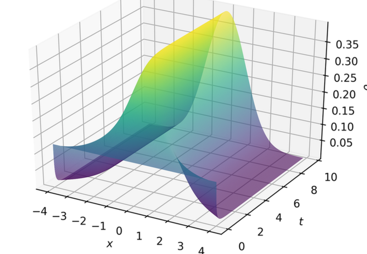
(a) Convergence to $\rho_{\infty}$ in time.

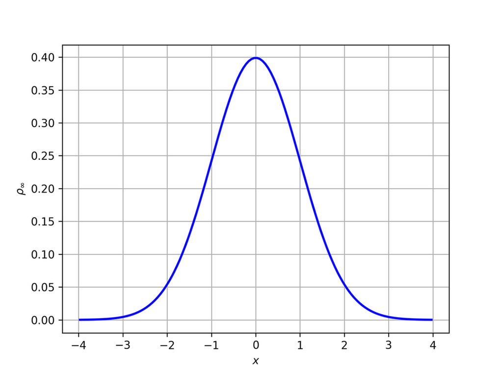
(b) Stationary state $\rho_{\infty}(x)$.

One dimension.

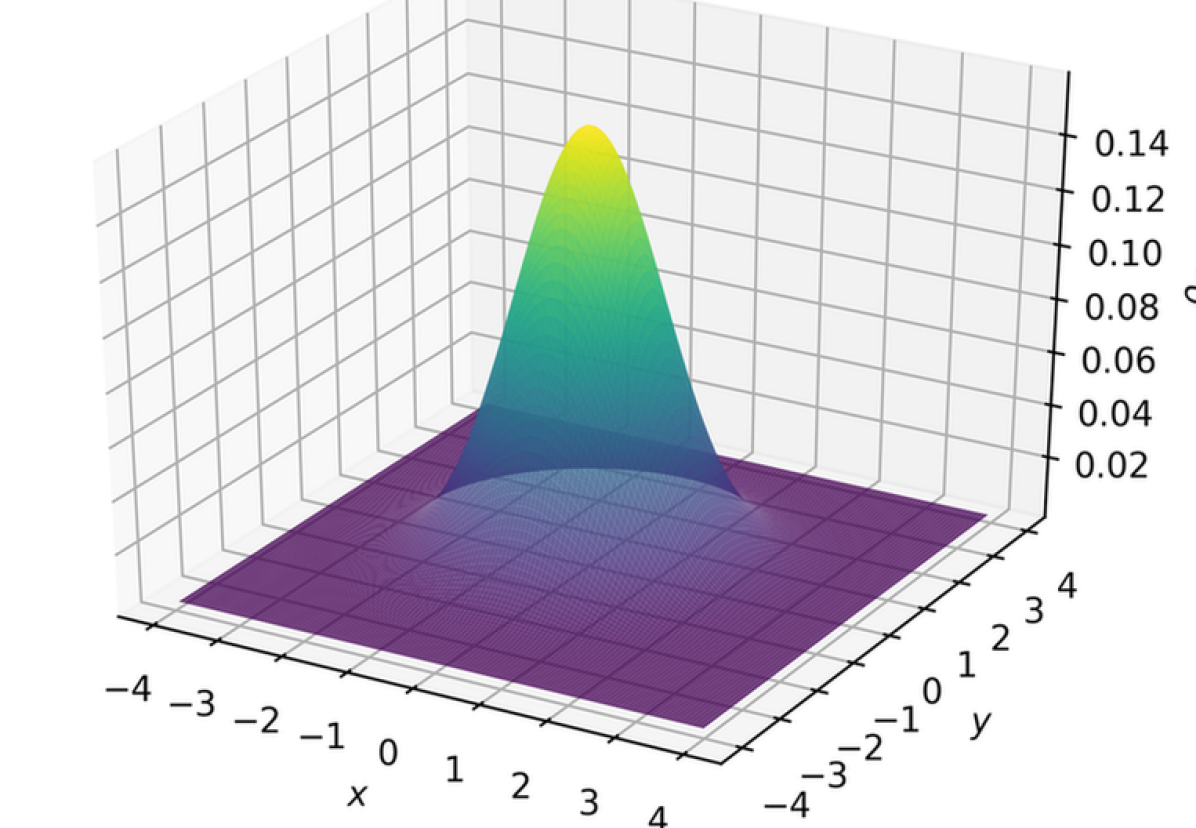
(c) Stationary state $\rho_{\infty}(x)$.

Two dimensions.

Figure 3: Stationary state of the non-local Fokker-Planck equation (6.11) with $D=1$, equivalent to that of the linear Fokker-Planck equation (6.8) due to the symmetry of the initial datum about the origin.

The confining potential of (6.8) can be replaced by an equal interaction potential, permitting the validation of the interaction component of the schemes. The new equation involves a non-local term but will have the same solution as the linear Fokker-Planck Equation for all initial datum which is symmetric about the origin, see Figure 3. This non-local Fokker-Planck Equation

$$H(\rho)=D(\rho\log(\rho)-\rho),\quad V(\mathbf{x})=0,\quad W(\mathbf{x})=\frac{|\mathbf{x}|^{2}}{2},$$ (6.11)

for $D>0$, ought to display the same analytical solution (6.10), the same steady state (6.9) and the same order of convergence to equilibrium as the local case. In the analytic setting, with centred initial datum, the $L_{1}$ difference $\|\rho(t,\mathbf{x})-\rho_{\infty}(\mathbf{x})\|_{L_{1}}$ is expected to decrease exponentially with order $\mathcal{O}(-2t)$. Furthermore, the relative entropy $E(\rho)-E(\rho_{\infty})$ should decrease with $\mathcal{O}(-4t)$ [60].

To validate the convergence of the sweeping dimensional splitting schemes, we validate the evolution of a source solution of Eq. 6.11 in two dimensions against the analytical solution (6.10), in the same fashion as Sections 6.2 and 6.3. The validation of the solution to Eq. 6.8 has also been included for comparison. Tables 17 and 18 demonstrate the second-order convergence using S1 for (6.8) and (6.11) respectively. Tables 19 and 20 show the corresponding (better than) first-order convergence using S2.

$\Delta t$	$\Delta x$	$\Delta y$	Error	Order
$2^{-4}$	$2^{-1}$	$2^{-1}$	0.0130193017	—
$2^{-6}$	$2^{-2}$	$2^{-2}$	0.0033748735	1.9477467433
$2^{-8}$	$2^{-3}$	$2^{-3}$	0.0008538822	1.9827243883
$2^{-10}$	$2^{-4}$	$2^{-4}$	0.0002153366	1.9874436476
$2^{-12}$	$2^{-5}$	$2^{-5}$	0.0000542630	1.9885519609

Table 17: Errors and orders of convergence for the solution to the linear Fokker-Planck equation (6.8) in two dimensions with S1. $D=1.0$, $t_{\mathrm{initial}}=2.0$, $t_{\mathrm{final}}=3.0$, $L=5.0$.

$\Delta t$	$\Delta x$	$\Delta y$	Error	Order
$2^{-6}$	$2^{-1}$	$2^{-1}$	0.0128997621	—
$2^{-8}$	$2^{-2}$	$2^{-2}$	0.0033440967	1.9476559875
$2^{-10}$	$2^{-3}$	$2^{-3}$	0.0008446799	1.9851398626
$2^{-12}$	$2^{-4}$	$2^{-4}$	0.0002133594	1.9851187830
$2^{-14}$	$2^{-5}$	$2^{-5}$	0.0000537499	1.9889523045

Table 18: Errors and orders of convergence for the solution to the non-local Fokker-Planck equation (6.11) in two dimensions with S1. $D=1.0$, $t_{\mathrm{initial}}=2.0$, $t_{\mathrm{final}}=3.0$, $L=5.0$.

$\Delta t$	$\Delta x$	$\Delta y$	Error	Order
$2^{-1}$	$2^{-1}$	$2^{-1}$	0.0126781382	—
$2^{-2}$	$2^{-2}$	$2^{-2}$	0.0035203530	1.8485509035
$2^{-3}$	$2^{-3}$	$2^{-3}$	0.0009623843	1.8710350515
$2^{-4}$	$2^{-4}$	$2^{-4}$	0.0002759015	1.8024599428
$2^{-5}$	$2^{-5}$	$2^{-5}$	0.0000804105	1.7786959505

Table 19: Errors and orders of convergence for the solution to the linear Fokker-Planck equation (6.8) in two dimensions with S2. $D=1.0$, $t_{\mathrm{initial}}=2.0$, $t_{\mathrm{final}}=3.0$, $L=5.0$.

$\Delta t$	$\Delta x$	$\Delta y$	Error	Order
$2^{-1}$	$2^{-1}$	$2^{-1}$	0.0126777040	—
$2^{-2}$	$2^{-2}$	$2^{-2}$	0.0035197973	1.8487292513
$2^{-3}$	$2^{-3}$	$2^{-3}$	0.0009618213	1.8716515859
$2^{-4}$	$2^{-4}$	$2^{-4}$	0.0002753364	1.8045732416
$2^{-5}$	$2^{-5}$	$2^{-5}$	0.0000798789	1.7853077858

Table 20: Errors and orders of convergence for the solution to the non-local Fokker-Planck equation (6.11) in two dimensions with S2. $D=1.0$, $t_{\mathrm{initial}}=2.0$, $t_{\mathrm{final}}=3.0$, $L=5.0$.

To validate the energy dissipation properties of the schemes, we studied the convergence in time of Gaussian initial datum in both problems to the numerical steady state, verifying the agreement between the local and the non-local settings. Convergence to the known dissipation rates upon refinement of the mesh was verified as well — see Figure 4 for the two-dimensional case.

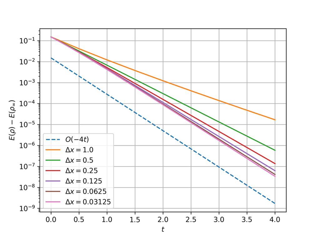
(a) S1.

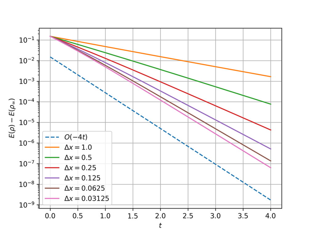
(b) S2.

Figure 4: Dissipation of the discrete energy $E_{\Delta}$ in the convergence to the stationary state of the non-local Fokker-Planck equation (6.11) in two dimensions. Note the slopes approach $\mathcal{O}(-4t)$ as the mesh is refined. $\Delta t=\Delta x$, $D=1.0$, $L=5.0$.

To further the discussion, we consider a non-linear diffusion case also. Replacing the linear term on (6.8) by the porous medium equivalent yields a non-linear Fokker-Planck Equation

$$H(\rho)=\frac{D}{m-1}\rho^{m},\quad V(\mathbf{x})=\frac{|\mathbf{x}|^{2}}{2},\quad W(\mathbf{x})=0,$$ (6.12)

for $D>0,m>1$. Again, regardless of initial datum this equation exhibits a globally stable steady state, see Figure 6.

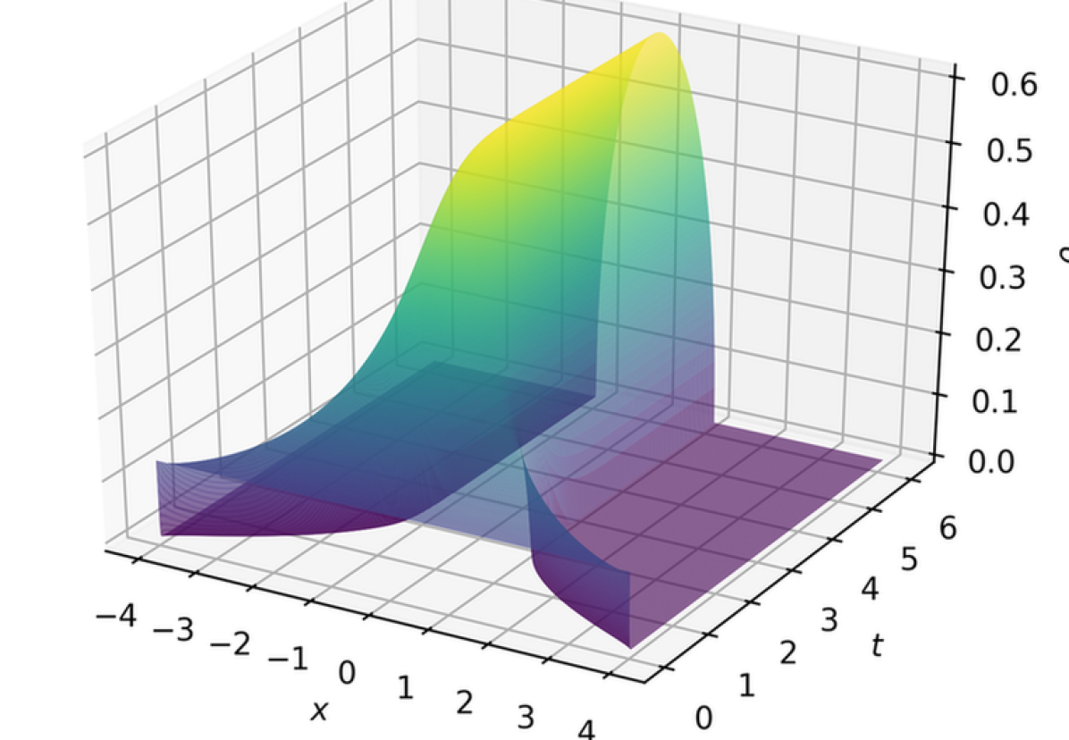
(a) Convergence to $\rho_{\infty}$ in time.

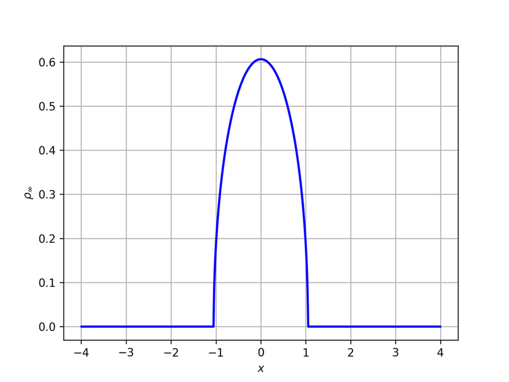
(b) Stationary state $\rho_{\infty}(x)$.

One dimension.

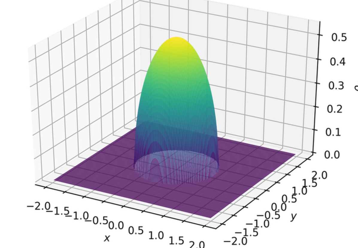
(c) Stationary state $\rho_{\infty}(x)$.

Two dimensions.

Figure 6: Stationary state of the non-linear Fokker-Planck equation (6.12) with $D=1,m=3$.

The regularity of the steady solution is once again controlled by the exponent $m$, and so is the rate of convergence to the stationary profile. In one dimension, for symmetric initial datum, the $L_{1}$ difference $\|\rho(t,\mathbf{x})-\rho_{\infty}(\mathbf{x})\|_{L_{1}}$ and the relative entropy $E(\rho)-E(\rho_{\infty})$ dissipate with $\mathcal{O}(-(m+1)t)$ and $\mathcal{O}(-2(m+1)t)$ respectively [28]. Similar verifications were performed — see Figure 7 for $m=3$.

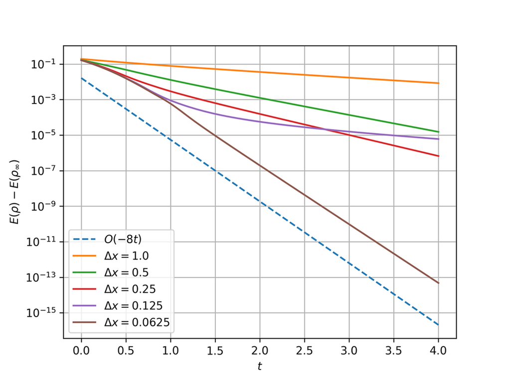
(a) S1.

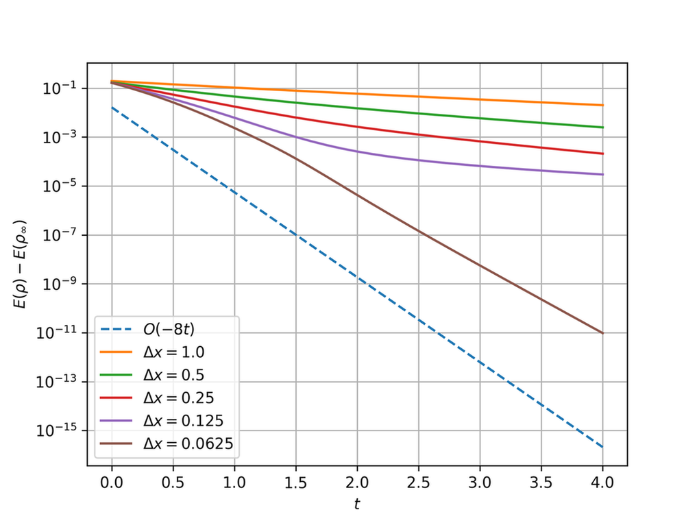
(b) S2.

Figure 7: Dissipation of the discrete energy $E_{\Delta}$ in the convergence to the stationary state of the non-linear Fokker-Planck equation (6.12) with exponent $3$ in one dimension. Note the slopes approach $\mathcal{O}(-8t)$ as the mesh is refined. $\Delta t=\Delta x$, $D=1.0$, $m=3.0$, $L=5.0$.

7 Numerical Experiments with S2

This concluding section presents a selection of experiments which aim to showcase some interesting problems which can be solved with the S2 scheme. First, we consider steady state problems with a variety of confining potentials. Later on, we discuss equations whose solutions display metastability in their convergence to equilibrium. Finally, we study a phase transition driven by noise in a kinetic system by constructing the stable branch of the bifurcation diagram.

7.1 Convergence to Steady States

Section 6.4 concerned the convergence to globally stable stationary solutions. Beyond the standard Fokker-Planck setting, the equivalents of (6.8) and (6.12) with more intricate confining potentials may be considered. For instance, a bistable term yields

$$H(\rho)=D(\rho\log(\rho)-\rho),\quad V(\mathbf{x})=\frac{|\mathbf{x}|^{4}}{4}-\frac{|\mathbf{x}|^{2}}{2},\quad W(\mathbf{x})=0,$$ (7.1)

for $D>0$ in the linear diffusion case, which displays a globally stable steady state characterised by maxima at $|\mathbf{x}|=1$; see Figure 9.

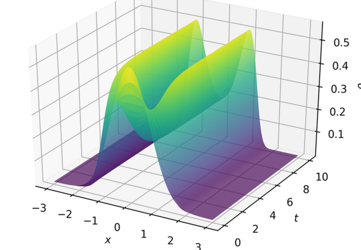
(a) Convergence to $\rho_{\infty}$ in time.

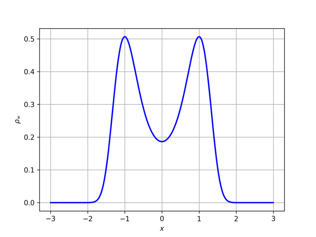
(b) Stationary state $\rho_{\infty}(x)$.

One dimension.

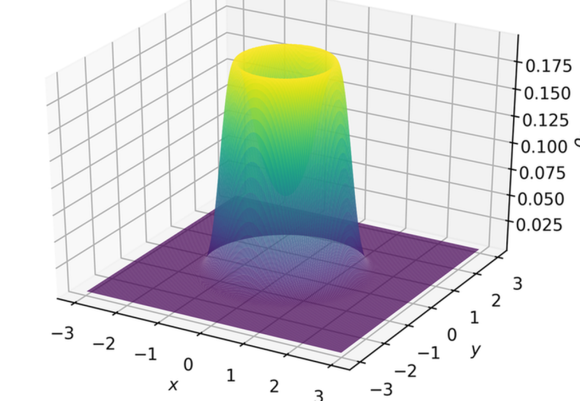
(c) Stationary state $\rho_{\infty}(x)$.

Two dimensions.

Figure 9: Stationary state of equation (7.1) with $D=0.25$. Note the maxima at $|\mathbf{x}|=1$.

(a) Convergence to $\rho_{\infty}$ in time.

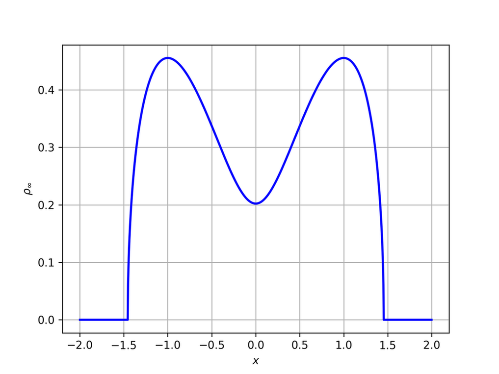
(b) Stationary state $\rho_{\infty}(x)$.

One dimension.

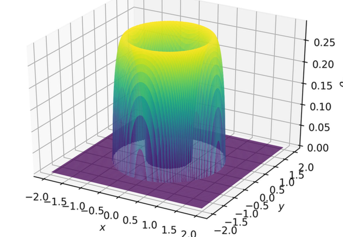
(c) Stationary state $\rho_{\infty}(x)$.

Two dimensions.

Figure 11: Stationary state of equation (7.2) with $D=1,m=3$.

In the non-linear setting, the equation reads:

$$H(\rho)=\frac{D}{m-1}\rho^{m},\quad V(\mathbf{x})=\frac{|\mathbf{x}|^{4}}{4}-\frac{|\mathbf{x}|^{2}}{2},\quad W(\mathbf{x})=0,$$ (7.2)

for $D>0,m>1$. The non-linear diffusion equivalent of (7.1) also has a unique stable steady state, compactly supported and characterised by maxima at $|\mathbf{x}|=1$ in two dimensions. In the one-dimensional setting, the steady state is only unique provided the diffusion coefficient $D$ is large [22]. Note that in two dimensions the stationary solution might not be simply connected — see Figure 11.

7.2 Metastability

We will now study the behaviour of a non-linear diffusion equation with an attractive interaction kernel:

$$H(\rho)=\frac{D}{m-1}\rho^{m},\quad V(\mathbf{x})=0,\quad W(\mathbf{x})=-\frac{1}{\sqrt{2\pi\sigma^{2}}}\exp\left(-\frac{|\mathbf{x}|^{2}}{2\sigma^{2}}\right),$$ (7.3)

for $D>0,m>1,\sigma>0$. This equation can exhibit a many-step convergence to equilibrium: rather than converging at a fixed rate, the energy dissipates in an alternating sequence of slow and fast timescales. Whilst the true steady state consists of a simply connected, compactly supported component, intermediate aggregates which depend on the initial datum can rapidly form. These aggregates will eventually merge but the rate of convergence can be arbitrarily slow if $\sigma$ is small.

Three examples are presented: Figure 12, where two aggregates are formed before reaching the final equilibrium; Figure 13, where three and then two aggregates are present before the steady state appears; and Figure 14, which shows the asymmetric aggregation in two dimensions. Note the intermediate plateaux on the energy landscapes, each corresponding to one of the many-aggregate states.

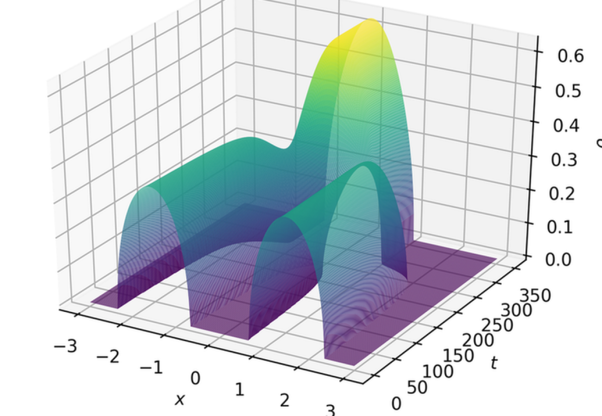
(a) Convergence to $\rho_{\infty}$ in time.

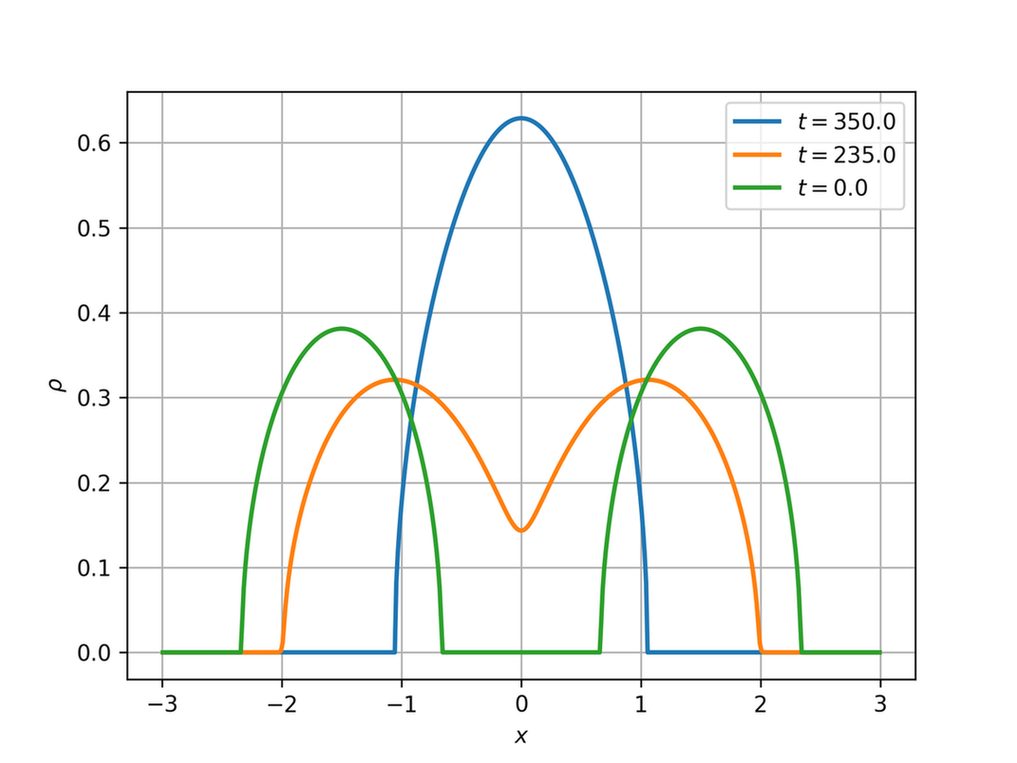
(b) Intermediate and stationary states.

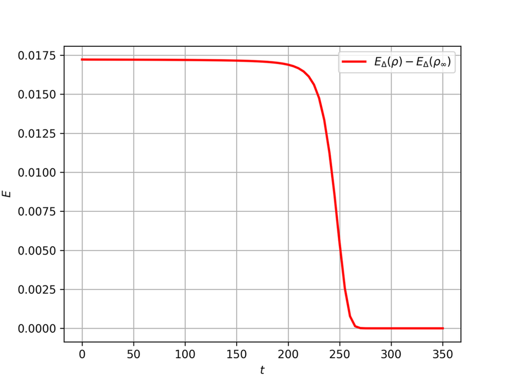
(c) Dissipation of the discrete energy.

Figure 12: Two-aggregate solution of equation (7.3) for $D=0.1,m=3,\sigma=0.5$.

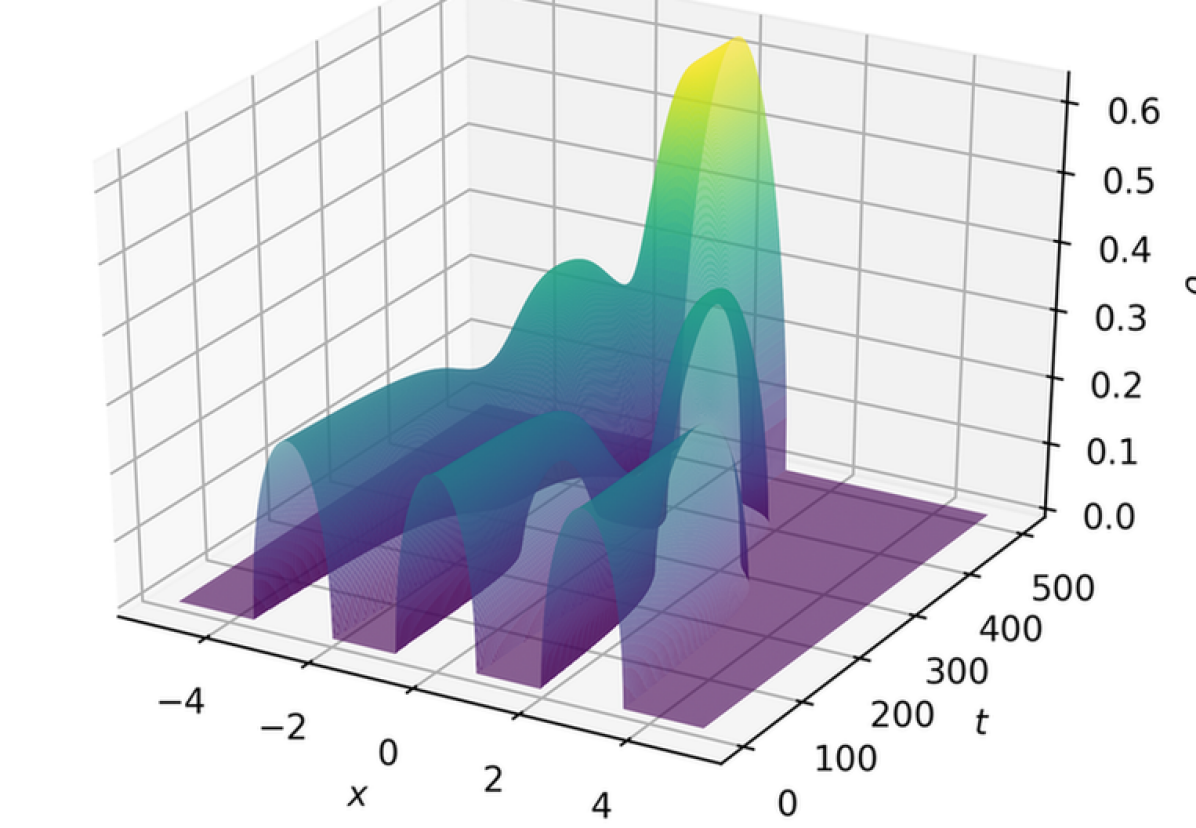
(a) Convergence to $\rho_{\infty}$ in time.

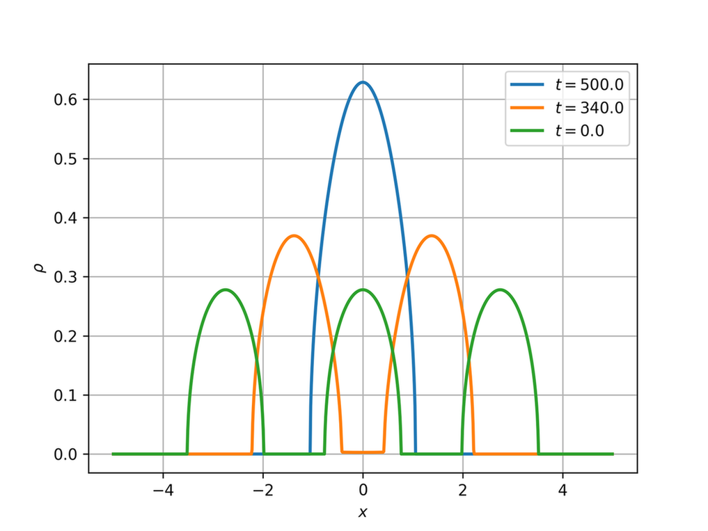
(b) Intermediate and stationary states.

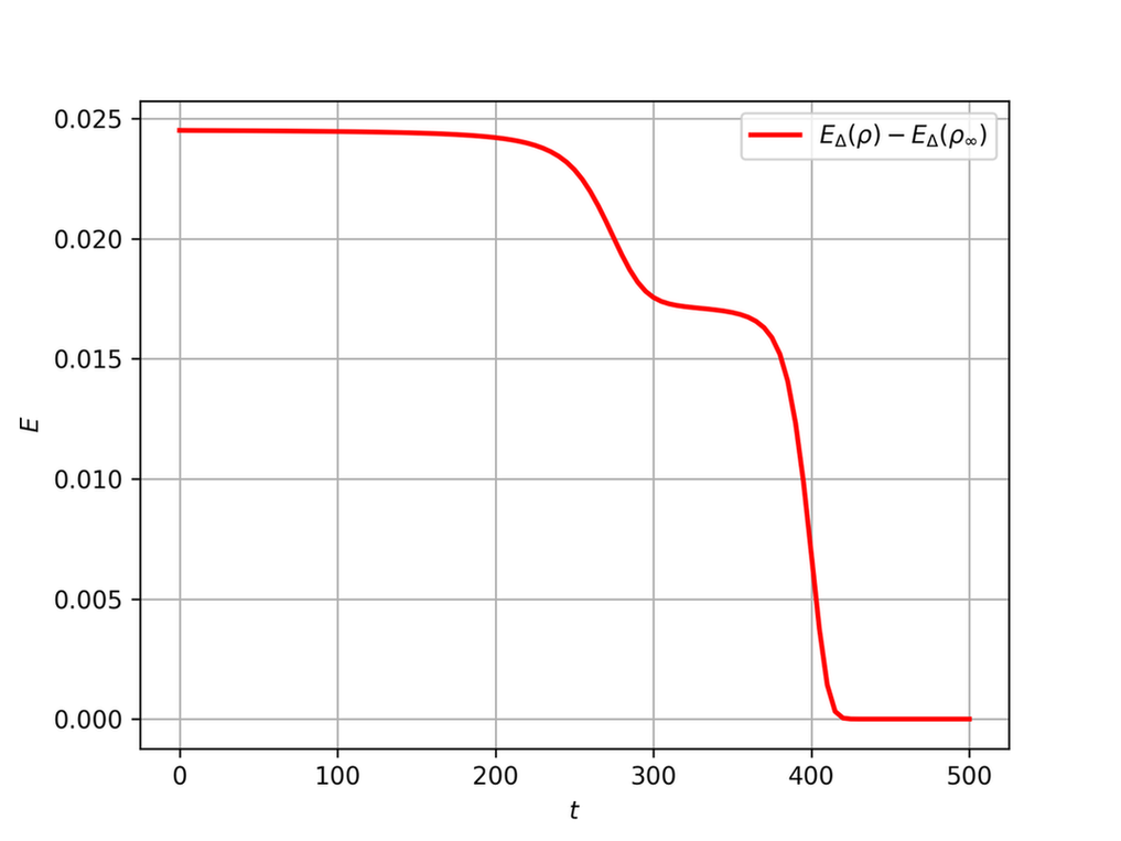
(c) Dissipation of the discrete energy.

Figure 13: Three-then-two-aggregate solution of equation (7.3) for $D=0.1,m=3,\sigma=0.5$.

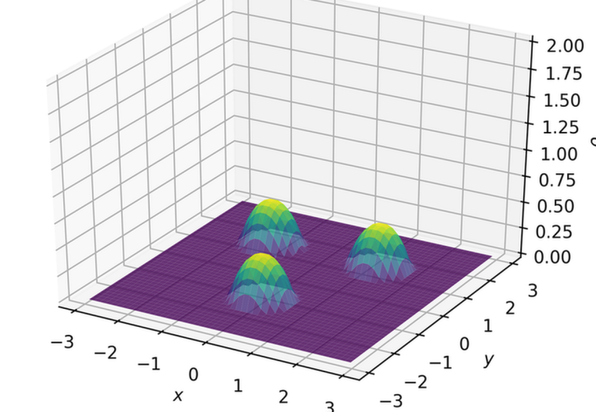
(a) $t=0$.

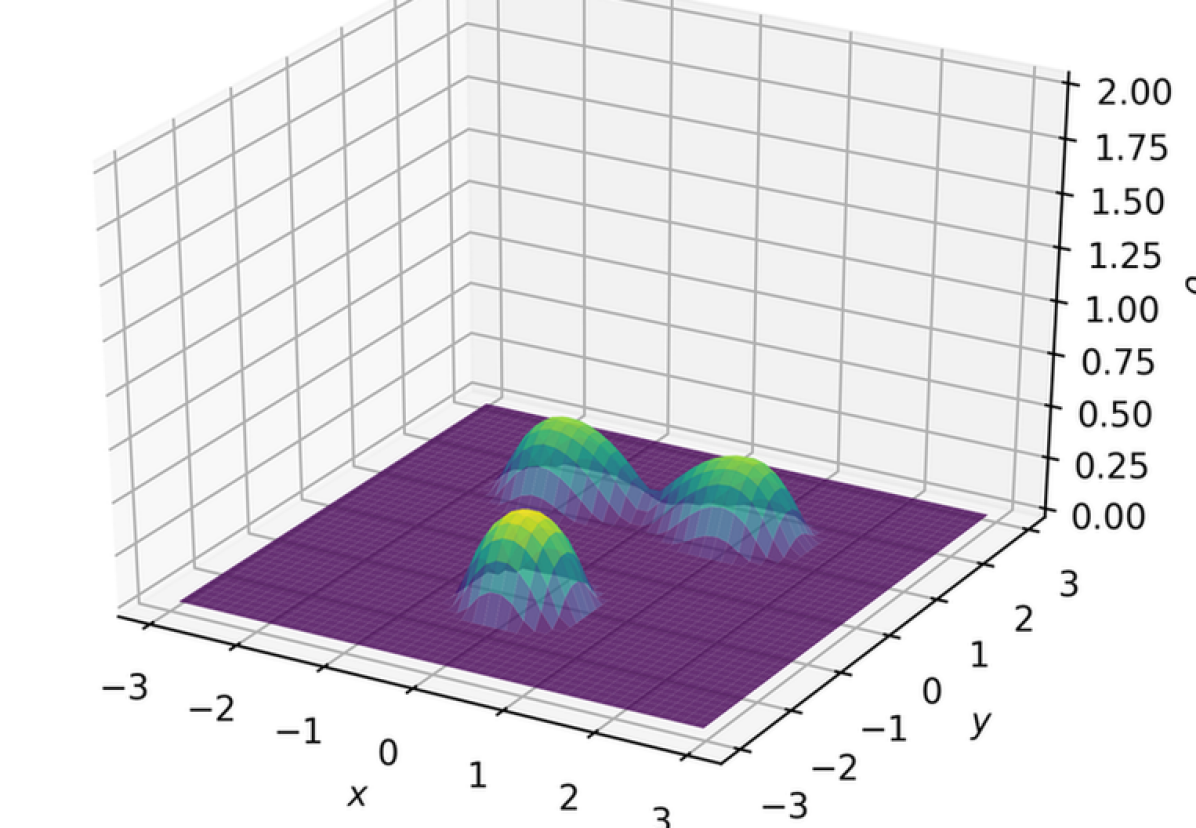
(b) $t=150$.

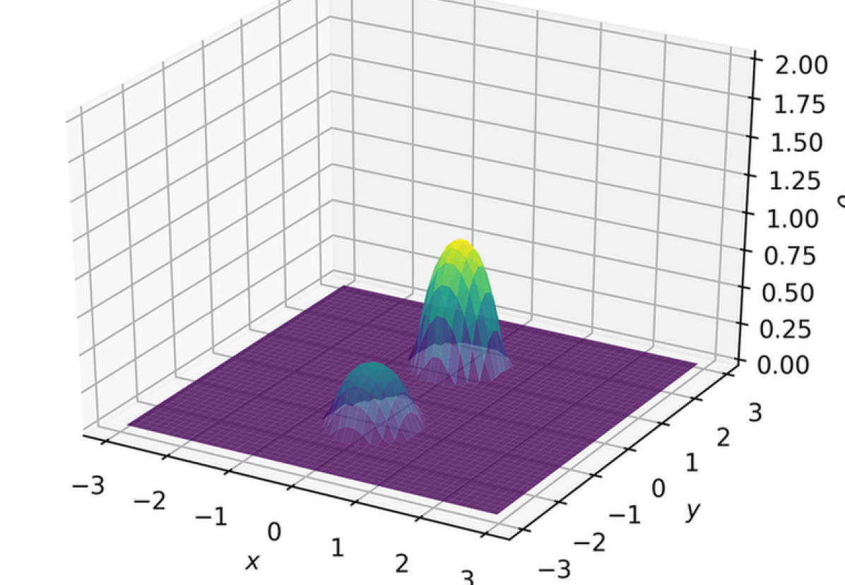
(c) $t=230$.

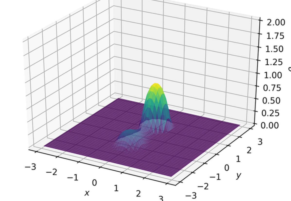
(d) $t=275$.

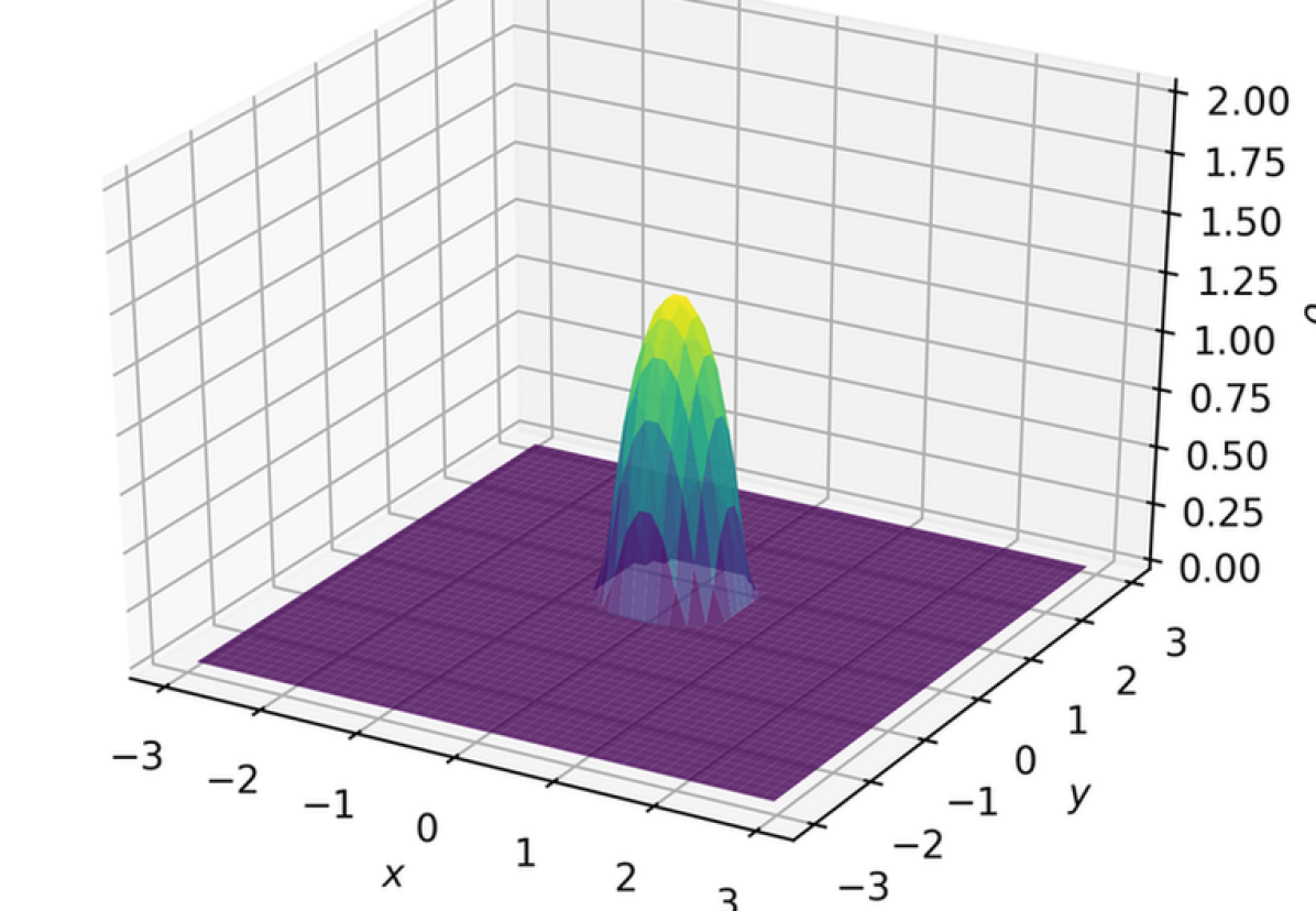
(e) $t=500$.

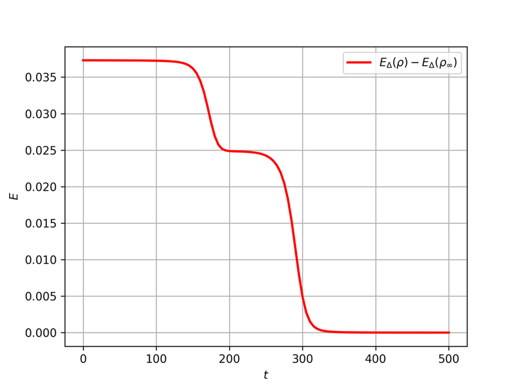
(f) Dissipation of the discrete energy.

Figure 14: Three-then-two-aggregate solution of equation (7.3) for $D=0.01,m=2,\sigma=0.5$ in two dimensions.

7.3 Homogeneous Noisy Kinetic Flocking

For the last example we will discuss a kinetic model for the velocity of self-propelled agents with a noisy tendency to flock:

$$H(\rho)=\sigma(\rho\log(\rho)-\rho),\quad V(\mathbf{x})=\alpha\left(\frac{|\mathbf{x}|^{4}}{4}-\frac{|\mathbf{x}|^{2}}{2}\right),\quad W(\mathbf{x})=\frac{|\mathbf{x}|^{2}}{2},$$ (7.4)

for $\sigma\geq 0,\alpha\geq 0$. For the sake of simplicity we retain the notation $\mathbf{x}$ even though the equation concerns velocities. The confinement potential represents the preference of the agents to move with speed one. The interaction kernel models the alignment tendency, and the diffusion component accounts for the noise in the system.

This model was studied at length in [61, 4, 32]. Among other things, the authors prove the existence of a phase transition in the system. Low values of $\sigma$ allow asymmetric initial conditions to flock, resulting in polarised steady states; the equation admits a symmetric steady state which is unstable and only realised for symmetric initial datum. Increasing the parameter beyond a critical threshold plunges the system into isotropic symmetry regardless of the initial condition.

The S2 scheme allowed us to solve the steady state problem of (7.4) for a large range of values of $\sigma$. The first moment of the steady state $\rho_{\infty}$,

$$\langle\mathbf{x}\rangle=\int\mathbf{x}\rho_{\infty}d\mathbf{x},$$ (7.5)

can be studied as a function of the noise strength $\sigma$, revealing whether the system is polarised or not. A sharp transition from the asymmetric polarised steady states to the isotropic setting can be seen on Figure 15 for the one-dimensional case. The centre of mass of the initial datum was shifted along the positive axis, resulting in the polarisation in that direction. By symmetry there is always another polarised steady state in the opposite direction.

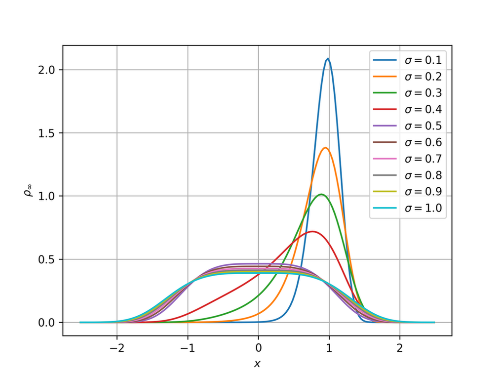
(a) Stationary state $\rho_{\infty}(x)$ for different values of $\sigma$.

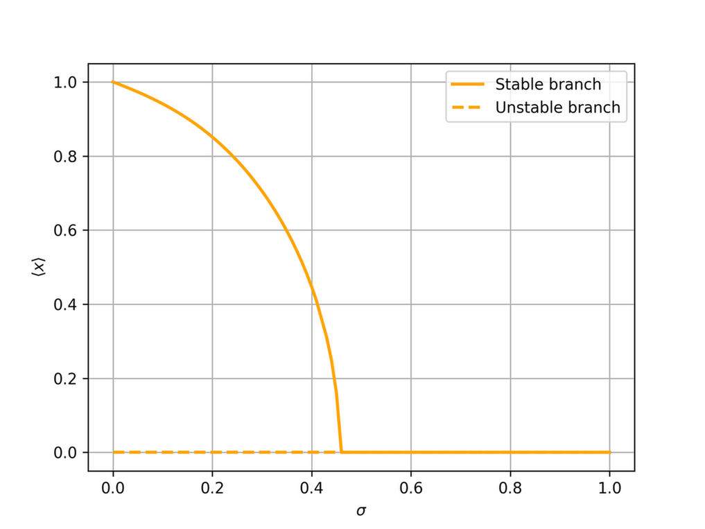
(b) Bifurcation diagram.

Figure 15: Stationary states and phase transition of (7.4) for $\alpha=1$ in one dimension.

The same phenomenon is observed in the two-dimensional setting, see Figure 17 and [4] for the analysis. The initial datum was shifted along the positive $x$ axis, resulting in the corresponding polarisation. Note that there is a rotationally symmetric family of polarised steady states. These states resemble a von Mises–Fisher distribution obtained for the Vicsek model ($\alpha=\infty$), see [41].

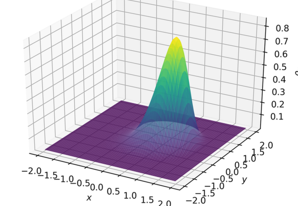
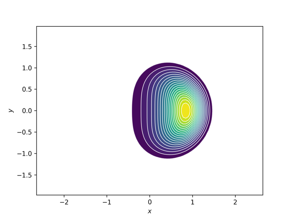
(a) Stationary state $\rho_{\infty}(x)$.

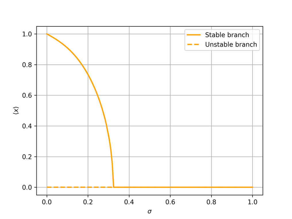
(b) Bifurcation diagram.

Figure 17: Stationary states and phase transition of (7.4) for $\alpha=1$ in two dimensions.

Finally, we discuss the phase transition for the non-linear diffusion case with and without a linear diffusion regularisation. This corresponds to:

$$H_{\varepsilon}(\rho)=\sigma\left(\frac{\rho^{m}}{m-1}+\varepsilon(\rho\log(\rho)-\rho)\right),\quad V(\mathbf{x})=\alpha\left(\frac{|\mathbf{x}|^{4}}{4}-\frac{|\mathbf{x}|^{2}}{2}\right),\quad W(\mathbf{x})=\frac{|\mathbf{x}|^{2}}{2},$$ (7.6)

for $\epsilon\geq 0,\sigma\geq 0,m>1,\alpha\geq 0$. Figure 18 shows the stationary states without regularisation as well as the bifurcation diagrams for $\varepsilon=0$ and $\varepsilon>0$. The case shown, $m=2$, leads to compactly supported stationary states with Lipschitz regularity at the boundary of the support, see Figure 18 (a). The regularisation numerically compensates the loss of spatial accuracy of the scheme due to the lack of smoothness of the solution, requiring fewer mesh points to adequately capture the behaviour around the critical point. Numerically we observe that the bifurcation diagram is continuous with respect to the regularisation parameter $\varepsilon$.

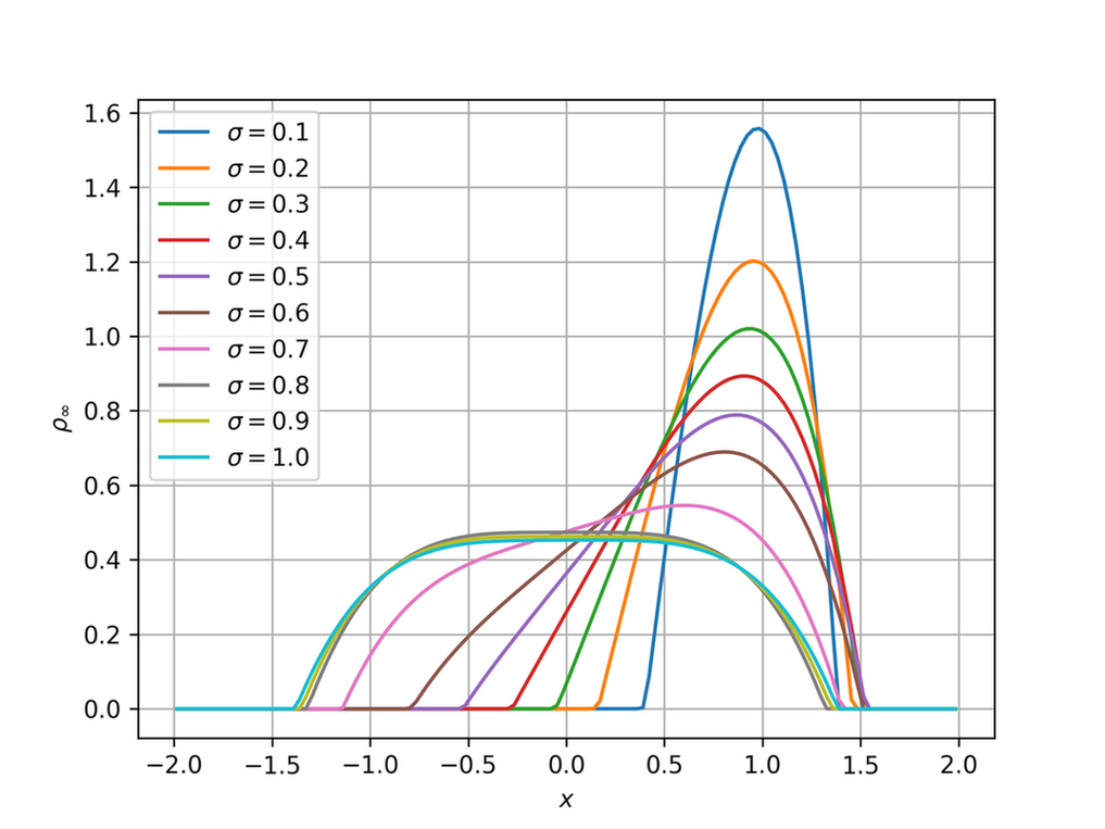
(a) Stationary states $\rho_{\infty}$ for $H_{0}(\rho)$ and varying $\sigma$.

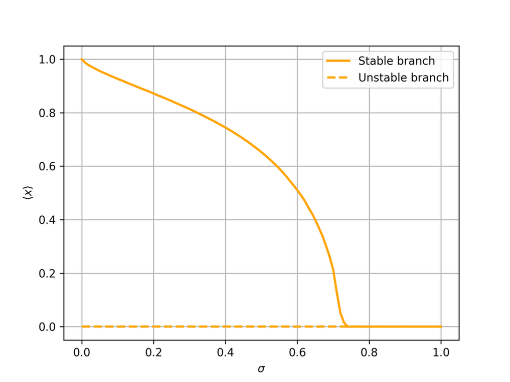
(b) Bifurcation diagram for $H_{0}(\rho)$.

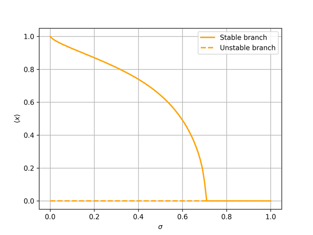
(c) Bifurcation diagram for $H_{\varepsilon}(\rho)$, with $\varepsilon=0.01$.

Figure 18: Stationary states and phase transition of (7.6) for $\alpha=1,m=2$ in one dimension.

References

- [1] L. Almeida, F. Bubba, B. Perthame, and C. Pouchol. Energy and implicit discretization of the Fokker-Planck and Keller-Segel type equations. arXiv:1803.10629 [math], Oct. 2018.
- [2] L. Ambrosio, N. Gigli, and G. Savare. Gradient Flows: In Metric Spaces and in the Space of Probability Measures. Lectures in Mathematics. ETH Zürich. Birkhäuser Basel, 2005.
- [3] A. Arnold and A. Unterreiter. Entropy decay of discretized fokker-planck equations I - Temporal semidiscretization. Computers & Mathematics with Applications, 46(10-11):1683–1690, Nov. 2003.
- [4] A. B. T. Barbaro, J. A. Cañizo, J. A. Carrillo, and P. Degond. Phase Transitions in a Kinetic Flocking Model of Cucker–Smale Type. Multiscale Model. Simul., 14(3):1063–1088, Jan. 2016.
- [5] J. Barré, P. Degond, and E. Zatorska. Kinetic Theory of Particle Interactions Mediated by Dynamical Networks. Multiscale Model. Simul., 15(3):1294–1323, Jan. 2017.
- [6] D. Benedetto, E. Caglioti, J. A. Carrillo, and M. Pulvirenti. A Non-Maxwellian Steady Distribution for One-Dimensional Granular Media. Journal of Statistical Physics, 91(5/6):979–990, 1998.
- [7] D. Benedetto, E. Caglioti, and M. Pulvirenti. A kinetic equation for granular media. ESAIM: M2AN, 31(5):615–641, 1997.
- [8] D. Benedetto, E. Caglioti, and M. Pulvirenti. A kinetic equation for granular media. ESAIM: M2AN, 33(2):439–441, Mar. 1999.
- [9] M. Bessemoulin-Chatard and F. Filbet. A Finite Volume Scheme for Nonlinear Degenerate Parabolic Equations. SIAM J. Sci. Comput., 34(5):B559–B583, Jan. 2012.
- [10] J. Bezanson, A. Edelman, S. Karpinski, and V. B. Shah. Julia: A Fresh Approach to Numerical Computing. SIAM Rev., 59(1):65–98, Jan. 2017.
- [11] A. Blanchet, V. Calvez, and J. A. Carrillo. Convergence of the Mass-Transport Steepest Descent Scheme for the Subcritical Patlak–Keller–Segel Model. SIAM J. Numer. Anal., 46(2):691–721, Jan. 2008.
- [12] F. Bolley, J. A. Cañizo, and J. A. Carrillo. Stochastic mean-field limit: Non-Lipschitz forces and swarming. Math. Models Methods Appl. Sci., 21(11):2179–2210, Nov. 2011.
- [13] C. Buet, S. Cordier, and V. D. Santos. A Conservative and Entropy Scheme for a Simplified Model of Granular Media. Transport Theory and Statistical Physics, 33(2):125–155, Jan. 2004.
- [14] C. Buet and S. Dellacherie. On the Chang and Cooper scheme applied to a linear Fokker-Planck equation. Communications in Mathematical Sciences, 8(4):1079–1090, 2010.
- [15] M. Burger, V. Capasso, and D. Morale. On an aggregation model with long and short range interactions. Nonlinear Analysis: Real World Applications, 8(3):939–958, July 2007.
- [16] M. Burger, J. A. Carrillo, and M.-T. Wolfram. A mixed finite element method for nonlinear diffusion equations. Kinetic & Related Models, 3(1):59–83, 2010.
- [17] M. Burger, R. Fetecau, and Y. Huang. Stationary States and Asymptotic Behavior of Aggregation Models with Nonlinear Local Repulsion. SIAM J. Appl. Dyn. Syst., 13(1):397–424, Jan. 2014.
- [18] V. Calvez and J. A. Carrillo. Volume effects in the Keller–Segel model: Energy estimates preventing blow-up. Journal de Mathématiques Pures et Appliquées, 86(2):155–175, Aug. 2006.
- [19] M. Campos Pinto, J. A. Carrillo, F. Charles, and Y.-P. Choi. Convergence of a linearly transformed particle method for aggregation equations. Numer. Math., 139(4):743–793, Aug. 2018.
- [20] J. A. Cañizo, J. A. Carrillo, and F. S. Patacchini. Existence of Compactly Supported Global Minimisers for the Interaction Energy. Arch Rational Mech Anal, 217(3):1197–1217, Sept. 2015.
- [21] K. Carlsson, P. K. Mogensen, S. Villemot, S. Lyon, M. Gomez, C. Rackauckas, T. Holy, T. Kelman, D. Widmann, M. R. G. Macedo, T. A. Bojesen, T. Arakaki, S. Christ, S. Byrne, M. Lubin, D. Barton, C. Kwon, C. Lucibello, A. r. N. Riseth, and A. Levitt. JuliaNLSolvers/NLsolve.jl: V4.1.0. July 2019.
- [22] J. A. Carrillo, A. Chertock, and Y. Huang. A Finite-Volume Method for Nonlinear Nonlocal Equations with a Gradient Flow Structure. Commun. Comput. Phys., 17(01):233–258, Jan. 2015.
- [23] J. A. Carrillo, A. Colombi, and M. Scianna. Adhesion and volume constraints via nonlocal interactions determine cell organisation and migration profiles. Journal of Theoretical Biology, 445:75–91, May 2018.
- [24] J. A. Carrillo, K. Craig, and F. S. Patacchini. A blob method for diffusion. Calc. Var., 58(2):53, Apr. 2019.
- [25] J. A. Carrillo, K. Craig, and Y. Yao. Aggregation-Diffusion Equations: Dynamics, Asymptotics, and Singular Limits. In N. Bellomo, P. Degond, and E. Tadmor, editors, Active Particles, Volume 2, pages 65–108. Springer International Publishing, Cham, 2019.
- [26] J. A. Carrillo, M. G. Delgadino, and A. Mellet. Regularity of Local Minimizers of the Interaction Energy Via Obstacle Problems. Commun. Math. Phys., 343(3):747–781, May 2016.
- [27] J. A. Carrillo, M. G. Delgadino, and F. S. Patacchini. Existence of ground states for aggregation-diffusion equations. Anal. Appl., 17(03):393–423, May 2019.
- [28] J. A. Carrillo, M. Di Francesco, and G. Toscani. Strict contractivity of the 2-Wasserstein distance for the porous medium equation by mass-centering. Proc. Amer. Math. Soc., 135(02):353–364, Feb. 2007.
- [29] J. A. Carrillo, B. Düring, D. Matthes, and D. S. McCormick. A Lagrangian Scheme for the Solution of Nonlinear Diffusion Equations Using Moving Simplex Meshes. J Sci Comput, 75(3):1463–1499, June 2018.
- [30] J. A. Carrillo, M. Fornasier, G. Toscani, and F. Vecil. Particle, kinetic, and hydrodynamic models of swarming. In G. Naldi, L. Pareschi, and G. Toscani, editors, Mathematical Modeling of Collective Behavior in Socio-Economic and Life Sciences, pages 297–336. Birkhäuser Boston, Boston, 2010.
- [31] J. A. Carrillo, M. P. Gualdani, and A. Jüngel. Convergence of an entropic semi-discretization for nonlinear Fokker-Planck equations in d. Publicacions Matemàtiques, 52:413–433, July 2008.
- [32] J. A. Carrillo, R. S. Gvalani, G. A. Pavliotis, and A. Schlichting. Long-Time Behaviour and Phase Transitions for the Mckean–Vlasov Equation on the Torus. Arch Rational Mech Anal, 235(1):635–690, Jan. 2020.
- [33] J. A. Carrillo, Y. Huang, and S. Martin. Explicit flock solutions for Quasi-Morse potentials. Eur. J. Appl. Math, 25(5):553–578, Oct. 2014.
- [34] J. A. Carrillo, R. J. McCann, and C. Villani. Kinetic equilibration rates for granular media and related equations: Entropy dissipation and mass transportation estimates. Rev. Matemática Iberoam., pages 971–1018, 2003.
- [35] J. A. Carrillo and J. S. Moll. Numerical Simulation of Diffusive and Aggregation Phenomena in Nonlinear Continuity Equations by Evolving Diffeomorphisms. SIAM J. Sci. Comput., 31(6):4305–4329, Jan. 2010.
- [36] J. A. Carrillo, H. Ranetbauer, and M.-T. Wolfram. Numerical simulation of nonlinear continuity equations by evolving diffeomorphisms. Journal of Computational Physics, 327:186–202, Dec. 2016.
- [37] J. S. Chang and G. Cooper. A practical difference scheme for Fokker-Planck equations. Journal of Computational Physics, 6(1):1–16, Aug. 1970.
- [38] L. Chayes, I. Kim, and Y. Yao. An Aggregation Equation with Degenerate Diffusion: Qualitative Property of Solutions. SIAM J. Math. Anal., 45(5):2995–3018, Jan. 2013.
- [39] D. Coppersmith and S. Winograd. Matrix multiplication via arithmetic progressions. J. Symb. Comput., 9(3):251–280, Mar. 1990.
- [40] K. Craig and A. L. Bertozzi. A blob method for the aggregation equation. Math. Comp., 85(300):1681–1717, Dec. 2015.
- [41] P. Degond, A. Frouvelle, and J.-G. Liu. Phase Transitions, Hysteresis, and Hyperbolicity for Self-Organized Alignment Dynamics. Arch Rational Mech Anal, 216(1):63–115, Apr. 2015.
- [42] J. Garnier, G. Papanicolaou, and T.-W. Yang. Large Deviations for a Mean Field Model of Systemic Risk. SIAM J. Finan. Math., 4(1):151–184, Jan. 2013.
- [43] J. Garnier, G. Papanicolaou, and T.-W. Yang. Consensus Convergence with Stochastic Effects. Vietnam J. Math., 45(1-2):51–75, Mar. 2017.
- [44] S. N. Gomes and G. A. Pavliotis. Mean Field Limits for Interacting Diffusions in a Two-Scale Potential. J Nonlinear Sci, 28(3):905–941, June 2018.
- [45] T. Goudon, S. Jin, and B. Yan. Simulation of fluid–particles flows: Heavy particles, flowing regime, and asymptotic-preserving schemes. Communications in Mathematical Sciences, 10(1):355–385, 2012.
- [46] D. D. Holm and V. Putkaradze. Formation of clumps and patches in self-aggregation of finite-size particles. Physica D: Nonlinear Phenomena, 220(2):183–196, Aug. 2006.
- [47] O. Junge, D. Matthes, and H. Osberger. A Fully Discrete Variational Scheme for Solving Nonlinear Fokker–Planck Equations in Multiple Space Dimensions. SIAM J. Numer. Anal., 55(1):419–443, Jan. 2017.
- [48] T. Kolokolnikov, J. A. Carrillo, A. Bertozzi, R. Fetecau, and M. Lewis. Emergent behaviour in multi-particle systems with non-local interactions. Physica D: Nonlinear Phenomena, 260:1–4, Oct. 2013.
- [49] P. M. Lushnikov, N. Chen, and M. Alber. Macroscopic dynamics of biological cells interacting via chemotaxis and direct contact. Phys. Rev. E, 78(6):061904, Dec. 2008.
- [50] D. Matthes and H. Osberger. Convergence of a variational Lagrangian scheme for a nonlinear drift diffusion equation. ESAIM: M2AN, 48(3):697–726, May 2014.
- [51] S. Motsch and E. Tadmor. Heterophilious Dynamics Enhances Consensus. SIAM Rev., 56(4):577–621, Jan. 2014.
- [52] L. Pareschi and M. Zanella. Structure Preserving Schemes for Nonlinear Fokker–Planck Equations and Applications. J Sci Comput, 74(3):1575–1600, Mar. 2018.
- [53] G. A. Pavliotis. Stochastic Processes and Applications, volume 60 of Texts in Applied Mathematics. Springer New York, New York, NY, 2014.
- [54] D. Ruelle. Statistical Mechanics: Rigorous Results. W. A. Benjamin, Inc., New York-Amsterdam, 1969.
- [55] J. Shen, J. Xu, and J. Yang. A New Class of Efficient and Robust Energy Stable Schemes for Gradient Flows. SIAM Rev., 61(3):474–506, Jan. 2019.
- [56] V. Strassen. Gaussian elimination is not optimal. Numer. Math., 13(4):354–356, Aug. 1969.
- [57] Z. Sun, J. A. Carrillo, and C.-W. Shu. A discontinuous Galerkin method for nonlinear parabolic equations and gradient flow problems with interaction potentials. Journal of Computational Physics, 352:76–104, Jan. 2018.
- [58] A.-S. Sznitman. Topics in propagation of chaos. In P.-L. Hennequin, editor, Ecole d’Eté de Probabilités de Saint-Flour XIX — 1989, volume 1464 of Lecture Notes in Mathematics, pages 165–251. Springer Berlin Heidelberg, Berlin, Heidelberg, 1991.
- [59] C. M. Topaz, A. L. Bertozzi, and M. A. Lewis. A Nonlocal Continuum Model for Biological Aggregation. Bull. Math. Biol., 68(7):1601–1623, Sept. 2006.
- [60] G. Toscani. Entropy production and the rate of convergence to equilibrium for the Fokker-Planck equation. Quart. Appl. Math., 57(3):521–541, Sept. 1999.
- [61] J. Tugaut. Phase transitions of McKean–Vlasov processes in double-wells landscape. Stochastics, 86(2):257–284, Mar. 2014.
- [62] J. L. Vazquez. The Porous Medium Equation. Oxford University Press, Oct. 2006.
- [63] C. Villani. Topics in Optimal Transportation. Number v. 58 in Graduate Studies in Mathematics. American Mathematical Society, Providence, RI, 2003.