The propagation of statistical errors in covariant density functional theory: ground state observables and single-particle properties.

Abstract

Statistical errors in ground state observables and single-particle properties of spherical even-even nuclei and their propagation to the limits of nuclear landscape have been investigated in covariant density functional theory (CDFT) for the first time. In this study we consider only covariant energy density functionals with non-linear density dependency. Statistical errors for binding energies and neutron skins significantly increase on approaching two-neutron drip line. On the contrary, such a trend does not exist for statistical errors in charge radii and two-neutron separation energies. The absolute and relative energies of the single-particle states in the vicinity of the Fermi level are characterized by low statistical errors ($\sigma(e_{i})\sim 0.1$ MeV). Statistical errors in the predictions of spin-orbit splittings are rather small. Statistical errors in physical observables are substantially smaller than related systematic uncertainties. Thus, at the present level of the development of theory, theoretical uncertainties at nuclear limits are dominated by systematic ones. Statistical errors in the description of physical observables related to the ground state and single-particle degrees of freedom are typically substantially lower in CDFT as compared with Skyrme density functional theory. The correlations between the model parameters are studied in detail. The parametric correlations are especially pronounced for the $g_{2}$ and $g_{3}$ parameters which are responsible for the density dependence of the model. The accounting of this fact potentially allows to reduce the number of free parameters of non-linear meson coupling model from six to five.

I INTRODUCTION

Although significant progress has been achieved over the years in the development of theoretical tools for the description of low-energy nuclear phenomena, some simplifications and approximations are still necessary because of the complexity of nuclear many-body problem and the impossibility of its exact solution for the systems with large number of particles. In addition, fine details of nuclear force and its dependence on density are still not fully resolved. As a result, it becomes necessary to estimate theoretical uncertainties in the description of physical observables Reinhard and Nazarewicz (2010); Dobaczewski et al. (2014); Agbemava et al. (2014). This is especially important when one deals with the extrapolations beyond the known regions, as, for example, in particle number or deformation, since experimental data which acts as a substitute of exact solution are not available there. Such estimates are also required for the evaluation of predictive power of the models and the robustness of their predictions. The need for such estimates has been clearly recognized by nuclear theory community as illustrated by a substantial number of the studies aiming at the quantification of theoretical uncertainties in nuclear structure, nuclear reactions and nuclear astrophysics (see Refs. Erler et al. (2012); Afanasjev et al. (2013); Gao et al. (2013); Agbemava et al. (2014); McDonnell et al. (2015); Martin et al. (2016); Mumpower et al. (2016); Lovell et al. (2017) and references quoted therein).

There are two types of theoretical uncertainties: systematic and statistical ones Brandt (2014); Dobaczewski et al. (2014). Systematic theoretical uncertainties emerge from underlying theoretical approximations. In the framework of density functional theory (DFT), there are two major sources of these approximations, namely, the range of interaction and the form of the density dependence of the effective interaction Bender et al. (2003); Boguta and Bodmer (1977). In the non-relativistic case one has zero range Skyrme and finite range Gogny forces and different density dependencies Bender et al. (2003); Peru and Martini (2014). A similar situation exists also in the relativistic case: point coupling and meson exchange models have an interaction of zero and of finite range, respectively Vretenar et al. (2005); Lalazissis et al. (2005, 2009); Nikšić et al. (2008). The density dependence is introduced either through an explicit dependence of the coupling constants Typel and Wolter (1999); Lalazissis et al. (2005); Nikšić et al. (2008) or via non-linear meson couplings Boguta and Bodmer (1977); Lalazissis et al. (2009). This ambiguity in the definition of the range of the interaction and its density dependence leads to several major classes of the covariant energy density functionals (CEDF) which were discussed in Ref. Agbemava et al. (2014).

It is necessary to recognize that precise quantification of systematic errors in the regions of nuclear chart for which experimental data is not available is not possible due to a number of reasons Dobaczewski et al. (2014); Agbemava et al. (2014). Thus, we prefer to use the notation systematic uncertainties (instead of systematic errors introduced in Ref. Dobaczewski et al. (2014)) which has more narrow meaning since they are defined with respect of selected set of the functionals (see introduction of Ref. Agbemava et al. (2014)).

An additional source of theoretical uncertainties is related to the details of the fitting protocol such as the choice of experimental data and the selection of adopted errors. It applies only to a given functional and the related theoretical uncertainties are called statistical errors Brandt (2014); Dobaczewski et al. (2014). Note that the selection of adopted errors is to a degree subjective, in particular, if one deals with quantities of different dimensions.

The covariant density functional theory (CDFT) represents a relativistic extension of the DFT framework to the nuclear many-body problem Vretenar et al. (2005). It exploits basic properties of QCD at low energies, in particular symmetries and the separation of scales LNP (2004). It provides a consistent treatment of the spin degrees of freedom and spin-orbit splittings Litvinova and Afanasjev (2011) and includes the complicated interplay between the large Lorentz scalar and vector self-energies induced on the QCD level by the in-medium changes of the scalar and vector quark condensates Cohen et al. (1992). In addition, CEDFs include nuclear magnetism Koepf and Ring (1989), i.e. a consistent description of currents and time-odd mean fields Afanasjev and Abusara (2010a), for which no new adjustable parameters are required because of Lorentz invariance. The CDFT has been successfully applied to the description of a large variety of nuclear phenomena (see reviews in Refs. Vretenar et al. (2005); Meng et al. (2006); Nikšić et al. (2011); RDF (2016)).

However, only recently systematic efforts have been undertaken to quantify theoretical uncertainties in the description of physical observables within the CDFT framework. Systematic uncertainties, their sources and their propagation to the extremes of neutron number have been studied globally for the ground state masses, deformations, two-particle separation energies, charge radii and neutrons skins of even-even nuclei, as well as for the positions of drip lines in Refs. Afanasjev et al. (2013); Agbemava et al. (2014); Afanasjev et al. (2015); Agbemava et al. (2015, 2016); Afanasjev and Agbemava (2016). In Ref. Agbemava et al. (2015) systematic uncertainties in the predictions of the ground state properties of superheavy nuclei have been investigated. Above mentioned investigations were restricted to even-even nuclei which are either spherical or have only even-multipole deformations in the ground state. This restriction has been removed in Refs. Agbemava et al. (2016); Agbemava and Afanasjev (2017) in which the global studies of octupole deformed nuclei and related systematic uncertainties in their description have been performed. The investigations of systematic uncertainties have also been carried out for excited states such as inner fission barriers in superheavy nuclei (Ref. Agbemava et al. (2017)), deformed one-quasiparticle states in odd-mass actinides Afanasjev and Shawaqfeh (2011); Dobaczewski et al. (2015) and rotational states in even-even and odd-mass actinides (Ref. Afanasjev and Abdurazakov (2013)).

Although impressive amount of data on systematic uncertainties in the description of physical observables in the CDFT has been collected within last few years, very little is known about related statistical errors. So far, they have been investigated only for potential energy curves in a single superheavy nucleus for two CEDFs in Ref. Agbemava et al. (2017). To fill this gap in our knowledge of the performance of CEDFs, the present manuscript aims on a systematic study of statistical errors in the description of the ground state and single-particle properties of spherical nuclei.

A second goal of the present investigation is to establish the correlations between the CEDF parameters and to see whether these parameters are independent. Such correlations have not been studied systematically so far in the CDFT framework. Their presence affects statistical errors in the description of physical observables Debes and Dudek (2017). The removal of parametric correlations leads to the reduction of the dimensionality of the parameter hyperspace and to the decrease of statistical errors. The latter was illustrated in Ref. Debes and Dudek (2017) on the example of the study of statistical errors in the single-particle energies of spherical nuclei performed with Woods-Saxon potential.

So far, mostly the covariance analysis has been used in the studies of statistical errors for physical observables in the DFT framework (see, for example, Refs. Gao et al. (2013); Dobaczewski et al. (2014); Niksic et al. (2015); Haverinen and Kortelainen (2017). However, in the calculations of the covariance matrix a linearized least-square system in the vicinity of the minimum of objective function $\chi^{2}_{norm}$ is usually assumed Brandt (2014). This means that the covariance analysis assumes that full information about statistical errors is contained in the derivatives taken at the optimum parametrization and ignores potential non-linear dependence of the observables on the coupling constants in the parts of the parameter hyperspace away from the optimum parametrization. However, there is no guarantee that linear approximation is valid for non-linear problems in the region of the parameter hyperspace away from the optimum parametrization (see Ref. Brandt (2014)). If that is a case the covariance matrix loses its validity Brandt (2014). A priori such non-linearities, which are present in the CDFT models, cannot be disregarded. For example, the analysis of the correlations between the $\alpha_{S}$ and $\alpha_{V}$ parameters in point coupling models performed in Ref. Bürvenich et al. (2004) clearly indicates their presence.

Thus, we use alternative approach based on the Monte-Carlo method in which randomly generated functionals are accepted/rejected based on the condition of Eq. (4) given in Sec. II below. As a result, the set of reasonable functionals is generated which is used for the calculations of statistical errors in the physical observables of interest (see Sec. II). The advantage of this method is that its outcome is defined by full parameter hyperspace used in the analysis (and not only by the neighborhood of optimum parametrization as in covariance analysis). This allows to take existing non-linearities between the parameters fully into account. Thus, the Monte-Carlo approach is free from above mentioned deficiencies of the covariance analysis. However, it is much more numerically time consuming than relatively simple covariance analysis and requires significant computational power. As a result, so far it was applied only to the analysis of statistical errors in the single-particle energies of phenomenological Woods-Saxon potential (see Ref. Debes and Dudek (2017)). Because of this reason we focus in the present exploratory study on the non-linear (NL) CEDFs which are characterized by the minimum number of the parameters (and, as a consequence, by minimal dimensionality of the parameter hyperspace) among the state-of-the-art CEDFs. Their six parameters are the mass $m_{\sigma}$ and coupling constant $g_{\sigma}$ of the $\sigma$-meson, the coupling constant $g_{\omega}$ of the $\omega$-meson, the coupling constant $g_{\rho}$ of the $\rho$ meson which is responsible for the isovector channel of the functional and the coupling constants $g_{2}$ and $g_{3}$ which define the density dependence of the functional.

The paper is organized as follows. Section II describes the details of the analysis of statistical errors. Fitting protocols and related theoretical uncertainties are discussed in Sec. III. The ranges of the parameters and parametric correlations in the functionals are discussed in Sec. IV. Statistical errors in the description of the ground state observables of spherical even-even nuclei and their propagation towards neutron drip line are investigated in Sec. V. Sec. VI is devoted to the discussion of statistical errors in the description of single-particle energies and their consequences for the predictions at the extremes of neutron number and charge. Note that statistical errors discussed in Secs. V and VI are compared with available systematic uncertainties estimated previously in Refs. Afanasjev et al. (2013); Agbemava et al. (2014, 2015); Afanasjev and Agbemava (2016). Finally, Sec. VII summarizes the results of our work.

II Statistical errors and the details of the calculations

The normalized objective function is defined for model having $N_{par}$ adjustable parameters ${\bf p}=(p_{1},p_{2},...,p_{N_{par}})$ as

$$\chi^{2}_{norm}({\bf p})=\frac{1}{s}\sum_{i=1}^{N_{type}}\sum_{j=1}^{n_{i}}\left(\frac{O_{i,j}({\bf p})-O_{i,j}^{exp}}{\Delta O_{i,j}}\right)^{2}$$ (1)

where

$$s=\frac{\chi^{2}({\bf p}_{0})}{N_{data}-N_{par}}$$ (2)

is global scale factor (Birge factor Birge (1932)) defined at the minimum of the penalty function (optimum parametrization ${\bf p}_{0}$) which leads to the average $\chi^{2}({\bf p}_{0})$ per degree of freedom equal to one Dobaczewski et al. (2014) and

$$N_{data}=\sum_{i=1}^{N_{type}}n_{i}$$ (3)

is the total number of data points of different types. Here, $N_{type}$ stands for the number of different data types. The calculated and experimental/empirical values of physical observable $j$ of the $i-$th type are represented by $O_{i,j}({\bf p})$ and $O^{exp}_{i,j}$, respectively. $\Delta O_{i,j}$ is adopted error for physical observable $O_{i,j}$. These quantities for the functionals under study are summarized in Table 1.

The acceptable functionals are defined from the condition Dobaczewski et al. (2014)

$$\chi^{2}_{norm}({\bf p})\leq\chi^{2}_{norm}({\bf p}_{0})+1.$$ (4)

This condition specifies the ’physically reasonable’ domain around ${\bf p}_{0}$ in which the parametrization ${\bf p}$ provides a reasonable fit and thus can be considered as acceptable. This domain is the $N$-dimensional parameter hyperspace ${\bf P_{space}}=[p_{1_{min}}-p_{1_{max}},p_{2_{min}}-p_{2_{max}},...,p_{N_{min}}-p_{N_{max}}]$, where $p_{i_{min}}$ and $p_{i_{max}}$ represent the lower and upper boundaries for the variation of the $i-th$ parameter. These boundaries are defined in such a way that their further increase (for $p_{i_{max}}$) or decrease (for $p_{i_{min}}$) does not lead to additional points in parameter hyperspace which satisfy Eq. (4).

The numerical calculations are performed in the following way. New parametrizations ${\bf p}$ are randomly generated in the $N$-dimensional parameter hyperspace and they are accepted if the condition (4) is satisfied. Using the set $[{\bf p}_{1},{\bf p}_{2},...,{\bf p}_{M}]$ of $M$ accepted functional variations the calculations are performed for spherical nuclei in the Ca, Ni, Sn and Pb isotope chains from proton to neutron drip lines. For each nucleus the mean values of physical observables

$$\bar{O}_{i,j}=\frac{1}{M}\sum_{k=1}^{M}O_{i,j}({\bf p}_{k})$$ (5)

and their standard deviations

$$\sigma_{i,j}=\sqrt{\frac{1}{M}\sum_{k=1}^{M}[O_{i,j}({\bf p}_{k})-\bar{O}_{i,j}]^{2}}$$ (6)

are calculated. The latter serves as a measure of statistical error.

As mentioned in the introduction we consider here only non-linear meson coupling models which are characterized by the minimal set of the parameters amongst different classes of the CDFT models. In the meson-exchange models Serot and Walecka (1986); Lalazissis et al. (2009), the nucleus is described as a system of Dirac nucleons interacting via the exchange of mesons with finite masses leading to finite-range interactions. The starting point is a standard Lagrangian density Gambhir et al. (1990)

$$\mathcal{L} =\bar{\psi}\left[\gamma\cdot(i\partial-g_{\omega}\omega-g_{\rho}\vec{\rho}\,\vec{\tau}-eA)-m-g_{\sigma}\sigma\right]\psi$$

$$+\frac{1}{2}(\partial\sigma)^{2}-U(\sigma)-\frac{1}{4}\Omega_{\mu\nu}\Omega^{\mu\nu}+\frac{1}{2}m_{\omega}^{2}\omega^{2}$$

$$-\frac{1}{4}{\vec{R}}_{\mu\nu}{\vec{R}}^{\mu\nu}+\frac{1}{2}m_{\rho}^{2}\vec{\rho}^{\,2}-\frac{1}{4}F_{\mu\nu}F^{\mu\nu}$$ (7)

which contains nucleons described by the Dirac spinors $\psi$ with the mass $m$ and several effective mesons characterized by the quantum numbers of spin, parity, and isospin. They create effective fields in a Dirac equation, which corresponds to the Kohn-Sham equation Kohn and Sham (1965) of non-relativistic density functional theory. The density dependence is introduced into model via a non-linear meson coupling Boguta and Bodmer (1977)

$$U(\sigma)~{}=~{}\frac{1}{2}m_{\sigma}^{2}\sigma^{2}+\frac{1}{3}g_{2}\sigma^{3}+\frac{1}{4}g_{3}\sigma^{4}.$$ (8)

In simplest ansatz, the Lagrangian (II) contains as parameters the mass $m_{\sigma}$ of the $\sigma$ meson, the coupling constants $g_{\sigma}$, $g_{\omega}$, and $g_{\rho}$ as well as density dependent parameters $g_{2}$ and $g_{3}$. The masses $m$, $m_{\omega}$ and $m_{\rho}$ are typically fixed in non-linear meson coupling models. $e$ is the charge of the protons and it vanishes for neutrons.

The calculations have been performed using the spherical RHB code. The truncation of the basis is performed in such a way that all states belonging to the shells up to $N_{F}=20$ fermionic shells and $N_{B}=20$ bosonic shells are taken into account. In order to avoid the uncertainties connected with the definition of the size of the pairing window we use the separable form of the finite range Gogny pairing interaction introduced by Tian et al Tian et al. (2009) with the strength of pairing defined in Ref. Agbemava et al. (2014). This is also done for the consistency with previous global studies of systematic uncertainties in the description of physical observables within the CDFT framework Afanasjev et al. (2013); Agbemava et al. (2014); Afanasjev et al. (2015); Agbemava et al. (2015, 2016); Afanasjev and Agbemava (2016).

Table 1: Input data for fitting protocol of the NL5() CEDFs. The number $n_{i}$ of experimental (empirical) data points and adopted errors $\Delta O_{i,j}$ are presented for each type of data. The binding energies of the ¹⁶O, ⁴⁰Ca, ⁴⁸Ca, ⁷²Ni, ⁹⁰Zr, ¹¹⁶Sn, ¹²⁴Sn, ¹³²Sn, ²⁰⁴Pb, ²⁰⁸Pb, ²¹⁴Pb and ²¹⁰Po nuclei, the charge radii of ¹⁶O, ⁴⁰Ca, ⁴⁸Ca, ⁹⁰Zr, ¹¹⁶Sn, ¹²⁴Sn, ²⁰⁴Pb, ²⁰⁸Pb and ²¹⁴Pb nuclei as well as neutron skins of the ⁹⁰Zr, ¹¹⁶Sn, ¹²⁴Sn and ²⁰⁸Pb nuclei are used in the fitting protocol. In addition, employed empirical values $O_{i,j}$ for the properties of symmetric nuclear matter at saturation are provided; these are the density $\rho_{0}$, the energy per particle $E/A$, the incompressibility $K_{0}$ and the symmetry energy $J$. The columns 3-6 show only the changes with respect of the values provided in column 2.

	NL5(A)	NL5(B)	NL5(C)	NL5(D)	NL5(E)
1	2	3	4	5	6
1. Masses $E$ (MeV)
$n_{1}$	12
$\Delta E$ [MeV]	$0.001E$
2. Charge radii $r_{ch}$ (fm)
$n_{2}$	9
$\Delta r_{ch}$ [fm]	$0.002\,r_{ch}$
3. Neutron skin $r_{skin}$ (fm)
$n_{3}$	4		3 [no 90Zr]	0
$\Delta r_{skin}$ [fm]	$0.05\,r_{skin}$				see text
4. Nuclear matter properties
$n_{4}$	4
$E/A$ [MeV]	-16.0
$\Delta E/A$ [MeV]	$0.05E/A$
$\rho$ [fm-3]	0.153
$\Delta\rho$ [fm-3]	$0.1\rho$
$K_{0}$ [MeV]	250.0
$\Delta K_{0}$ [MeV]	$0.1K_{0}$	$0.025K_{0}$	$0.025K_{0}$	$0.025K_{0}$	$0.025K_{0}$
$J$ [MeV]	33.0
$\Delta J$ [MeV]	$0.1J$
Parameters of Eq. (1)
$N_{data}$	29		28	25
$N_{par}$	6
$N_{type}$	4			3

III Fitting protocols: an example of the origin of the uncertainties

Previous fits of the non-linear CEDFs have been performed in the RMF+BCS framework with simple pairing (see Refs. Reinhard et al. (1986); Rufa et al. (1988); Sharma et al. (1993); Lalazissis et al. (1997, 2009) for details). Since in the present work the RHB framework with separable pairing of finite range is used in fitting protocol for the first time, the investigation of the dependence of the optimum parametrization on the details of the fitting protocol is performed.

Table 2: Different functionals obtained in the present work. The details of the fitting protocols are discussed in the text. First part of the table shows the parameters of the functionals. Note that the masses of nucleon, $\omega$ and $\rho$ mesons are fixed at $m_{N}=939.0$ MeV, $m_{\omega}=782.6$ MeV and $m_{\rho}=763.0$ MeV, respectively. Related nuclear matter properties are displayed in the second part of the table. In addition to those quoted in Table 1, they also include the slope of the symmetry energy $L_{0}$. Total penalty function $\chi_{total}^{2}$ and the contributions to it coming from nuclear matter properties ($\chi_{NM}^{2}$), binding energies ($\chi_{E}^{2}$), charge radii ($\chi_{Rch}^{2}$) and neutron skins ($\chi_{Nskin}^{2}$) [and, in particular, the contribution of neutron skin of ⁹⁰Zr ($\chi_{Nskin(Zr)}^{2}$)] are presented in the last part of the table. Note that these contributions are given both in absolute values and in percentages [in parantheses] with respect of $\chi_{total}^{2}$. In addition, the penalty function per degree of freedom $\chi_{total}^{2}$/degree (Birge factor) is provided. For comparison, the NL1 Reinhard et al. (1986) (which is historically the first succesful CEDF) and NL3* Lalazissis et al. (2009) CEDFs and their nuclear matter properties are included in columns 2 and 3. The global performance of the NL3*, NL5(C), NL5(D) and NL5(E) functionals in the description of ground state properties of even-even nuclei is discussed in Appendix A.

	NL1	NL3*	NL5(A)	NL5(B)	NL5(C)	NL5(D)	NL5(E)
1. Parameters
$m_{\sigma}$	492.250	502.574200	516.993054	503.253177	502.481217	503.122989	503.298890
$g_{\sigma}$	10.1377	10.094400	10.165747	9.896631	9.900244	10.187753	10.263955
$g_{\omega}$	13.2846	12.806500	12.658290	12.457831	12.489590	12.940276	13.052487
$g_{\rho}$	4.9757	4.574800	4.277136	4.202553	4.318575	4.589814	4.582673
$g_{2}$	-12.1742	-10.809300	-8.350509	-10.925997	-10.821667	-10.858440	-10.976703
$g_{3}$	-36.2646	-30.148600	-19.260373	-28.502727	-28.27378	-30.993091	-32.006687
2. Nuclear matter properties
$E/A$	-16.42	-16.31	-16.25	-16.20	-16.24	-16.29	-16.27
$\rho_{0}$	0.152	0.150	0.146	0.150	0.150	0.150	0.150
$K_{0}$	211.11	258.27	318.42	259.22	260.673	256.50	252.96
$J$	43.46	38.68	34.92	34.92	35.925	38.87	38.93
$L_{0}$	140.07	122.68	108.85	108.33	112.31	123.98	124.96
2. Penalty function contributions
$\chi_{total}^{2}$			343.901	367.822	273.014	74.973	85.049
$\chi_{total}^{2}$/degree			14.95	15.99	12.41	3.9459	3.698
$\chi_{NM}^{2}$ ($\%$)			8.120 ( 2.3 $\%$)	2.626 (0.5 $\%$)	3.842 (1.1 $\%$)	4.434 (5.3 $\%$)	3.625 (3.5 $\%$)
$\chi_{E}^{2}$ ($(\%$)			128.318 (37.3 $\%$)	145.727 (39.6 $\%$)	111.550 (40.9 $\%$)	55.221 (73.7 $\%$)	51.231 (60.2 $\%$)
$\chi_{Rch}^{2}$ ($\%$)			34.231 ( 9.9 $\%$)	18.363 (5.0 $\%$)	16.124 (5.9 $\%$)	15.318 (20.4 $\%$)	16.802 (19.7 $\%$)
$\chi_{Nskin}^{2}$ ( $\%$)			173.235 (50.4 $\%$)	201.105 (54.6 $\%$)	141.498 (51.8 $\%$)	0 (0.0 $\%$)	13.390 (15.7 $\%$)
$\chi_{Nskin(Zr)}^{2}$($\%$)			76.071 (22.1 $\%$)	86.591 (23.5 $\%$)	0 (0.0 $\%$)	0 (0.0 $\%$)	1.178 (1.4 $\%$)

The starting point is the fitting protocol of the NL3* functional (see Ref. Lalazissis et al. (2009)). The types of the input data for this protocol and related adopted errors are summarized in column 2 of Table 1. The minimization within this protocol leads to optimum functional labeled NL5(A) (see Table 2). When considering the quality of the functional we take into account the ranges of the nuclear matter properties recommended for relativistic functionals in Ref. Dutra et al. (2014). These are $\rho_{0}\sim 0.15$ fm^-3, $E/A\sim-16$ MeV, $K_{0}=190-270$, $J=25-35$ MeV ($J=20-35$ MeV) and $L_{0}=25-115$ ($L_{0}=30-80$) for the SET2a (SET2b) sets of the constraints on the experimental/empirical ranges for the quantities of interest. As compared with the CEDF NL3*, the NL5(A) functional has better $J$ and $L_{0}$ values but much worse $K_{0}$ value. The analysis of the contributions of physical observables of different classes shows that $\chi^{2}_{total}$ is dominated by the contributions from 4 data points on neutron skins with the contribution of the single data point on the neutron skin of ⁹⁰Zr providing 22.1% of $\chi^{2}_{total}$. These large contributions from neutron skin data to $\chi^{2}_{total}$ clearly illustrate that these functionals cannot accurately describe presently adopted experimental values of $r_{skin}$ obtained by means of hadronic probes.

To compensate for too large value of $K_{0}$ and to force it to more acceptable value, the adopted error for $K_{0}$ has been reduced from 10% to 2.5% in the fitting protocol of the NL5(B) functional (see column 3 of Table 1). This functional and related nuclear matter properties as well as penalty function contributions are shown in Table 2. Its $E/A$, $\rho_{0}$ and $K_{0}$ values are close to the NL3* ones, but it has better symmetry energy $J$ and the slope of symmetry energy $L_{0}$. However, similar to NL5(A) it suffers from too large contribution of neutron skins (and especially, the one coming from ⁹⁰Zr) to $\chi^{2}_{total}$.

To reduce this problem, the neutron skin of ⁹⁰Zr has been dropped from the fitting protocol of the NL5(C) functional (see column 4 in Table 1.) This functional has $E/A$, $\rho_{0}$ and $K_{0}$ values similar to the ones of the NL3* and NL5(B) functionals (see Table 2). Its $J$ and $L_{0}$ values are better than those of the NL3* functional but slightly worse as compared with those of the NL5(B) one. However, the NL5(C) functional provides better description of binding energies and charge radii as compared with the NL5(A) and NL5(B) ones; these are physical observables which are precisely measured in experiment. On the other hand, it gives slightly worse description of neutron skins in the ¹¹⁶Sn, ¹²⁴Sn and ²⁰⁸Pb nuclei but as mentioned before this physical observable is characterized by substantial experimental uncertainties.

One can consider removing the neutron skins (as least reliable experimental data on finite nuclei) from the fitting protocol; this leads to the NL5(D) functional (see Table 2). It is characterized by a substantial reduction (by a factor of 2 as compared with the CEDF NL5(C)) of the error in the reproduction of experimental data on binding energies. However, for this functional the $J$ and $L_{0}$ values deviate more from recommended values as compared with the NL5(C) one.

Alternatively, one can use experimental errors (from Refs. Krasznahorkay et al. (1999); Yako et al. (2006); Tarbert et al. (2014)) as adopted errors for neutron skins which are substantially larger than adopted errors (5%) of the fitting protocol of the NL5(A-C) functionals (Table 1). This leads to the NL5(E) functional in which the impact of neutron skins on total $\chi^{2}_{total}$ is substantially reduced as compared with NL5(A-C) functionals. As a consequence, the nuclear matter properties of the NL5(D) and NL5(E) functionals are similar and they provide comparable description of binding energies and charge radii.

The results presented here clearly show that the selection of the fitting protocol (physical observables and related adopted errors) is to a degree subjective. Definitely the use of more experimental data of different types is expected to reduce this level of subjectivity but it cannot be completely eliminated. Since the Monte-Carlo analysis of statistical errors is numerically extremely time-consuming, we restrict our investigation of statistical errors of non-linear CEDFs to NL5(C) and NL5(A) functionals.

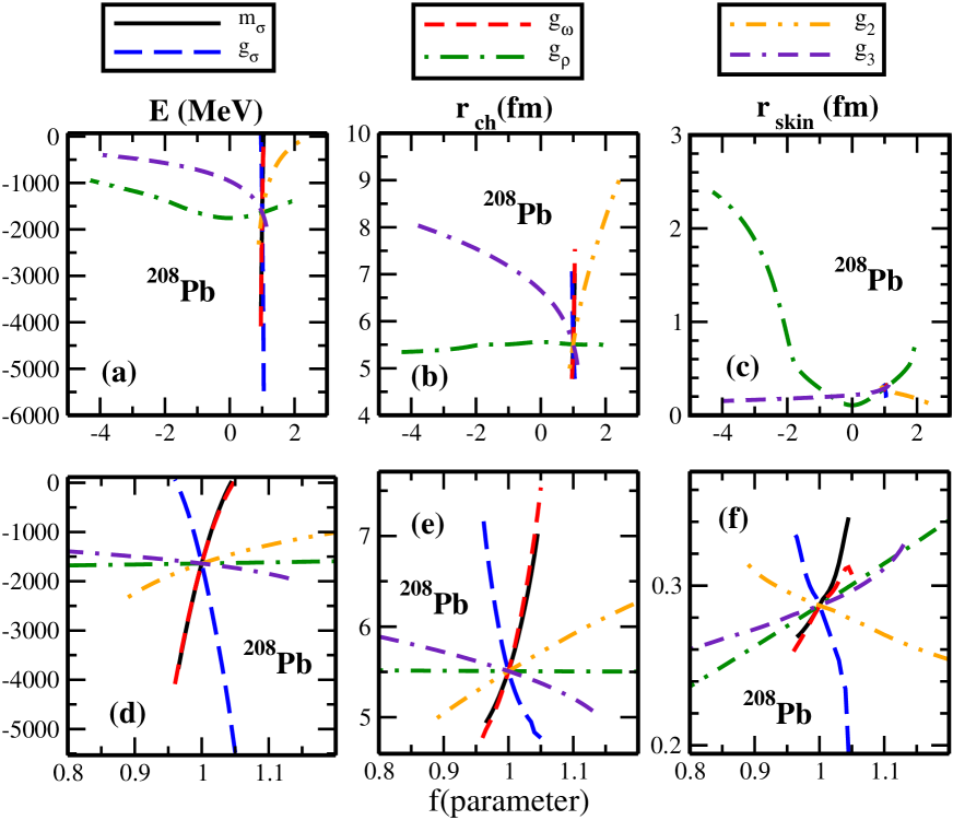
Figure 1: (Color online) The range of the variations of the parameters of the NL5(C) CEDF and related changes of physical observables such as total binding energy $E$ (left columns), charge radius $r_{ch}$ (central columns) and neutron skin $r_{skin}$ (right columns). Upper row shows the full range of the parameter variations, while the bottom panels magnify the region in the vicinity of optimum parametrization ($f_{i}=1.0$). On the one end, the range of parameters is limited by the condition that the total energy of the nucleus is negative. On the other end, it is defined by the collapse of numerical solution due to underlying numerical instabilities. For each line, only the indicated parameter is changing while the remaining parameters are kept at the values corresponding to optimum NL5(C) functional.

IV The ranges of the parameters and parametric correlations in the functionals

In meson exchange models the general features of the nuclei are dominated by the properties of the $\sigma$ and $\omega$ mesons which are responsible for intermediate range attraction and short range repulsion. They lead to attractive scalar $S$ and repulsive vector $V$ potentials with magnitudes of $S\approx-400$ MeV/nucleon and $V\approx+350$ MeV/nucleon Reinhard (1989); Ring (1996). Their sum defines the depth of nucleonic potential ($\sim-50$ MeV/nucleon).

Because of these large magnitudes, very small variations of the masses and coupling constants of these two mesons lead to substantial changes in binding energies (see Figs. 1a and d). Note that in this chapter instead of functional parameters $par_{i}$ we are using the ratio

$$f_{i}=\frac{par_{i}}{par_{i}^{opt}}$$ (9)

where $par_{i}^{opt}$ is the value of the parameter in the optimum functional and $i$ indicates the type of the parameter. This allows to better understand the range of the variations of the parameters and related parametric correlations in the functionals.

Coming back to Figs. 1a and d, one can see that $\pm 5$% change in the values of $m_{\sigma}$, $g_{\sigma}$ and $g_{\omega}$ leads to the changes of binding energies in the range of 2000-3000 MeV. Other physical observables used in the fitting protocols such as charge radii $r_{ch}$ also sensitevely depend on $f_{i}$ (see Figs. 1b and e). However, some flexibility in acceptable ranges of these parameters is provided by the fact that binding energies and charge radii have different dependencies on $f(m_{\sigma})$, $f(g_{\sigma})$ and $f(g_{\omega})$ (see Fig. 1).

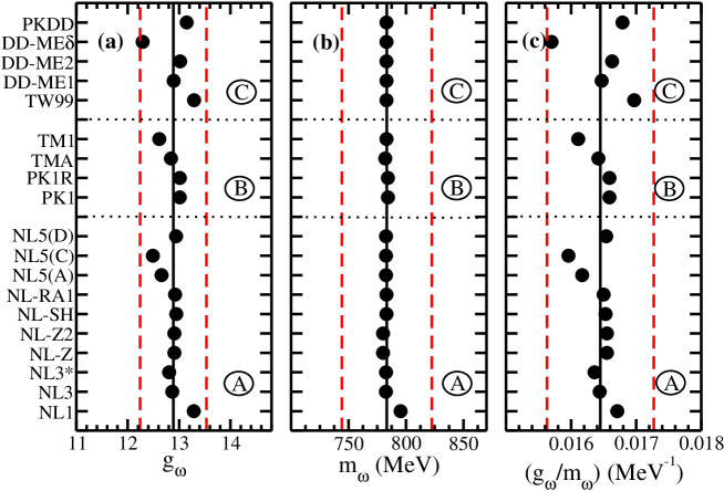
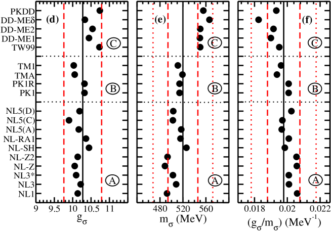
Figure 2: (Color online) The masses and coupling constants of the $\sigma$ and $\omega$ mesons in different CEDFs which contain meson exchange. They are combined into three groups dependent on how self- and mixed-couplings are introduced. Group A represents the parametrizations which include non-linear self-couplings only for the $\sigma$-meson. Group B contains the parametrizations which include self-couplings for the $\sigma$- and $\omega$-mesons (and $\rho-$mesons in the case of PK1R). Group C represents the parametrizations which include density-dependent meson-nucleon couplings for the $\sigma$-, $\omega$-, and $\rho$-mesons. Note that the mass $m_{\omega}$ of the $\omega$-meson is fixed at indicated values in all functionals except NL3, PK1 and PK1R. The parameters are taken from Refs. Reinhard et al. (1986) (NL1), Lalazissis et al. (1997) (NL3), Lalazissis et al. (2009) (NL3*), Rufa et al. (1988) (NL-Z), Bender et al. (1999) (NL-Z2), Sharma et al. (1993) (NL-SH), Rashdan (2001) (NL-RA1), Long et al. (2004) (PK1,PK1R), Ren and Toki (2001) (TMA), Sugahara and Toki (1994) (TM1), Typel and Wolter (1999) (TW99), Nikšić et al. (2002) (DD-ME1), Lalazissis et al. (2005) (DD-ME2), Roca-Maza et al. (2011) (DD-ME$\delta$), Long et al. (2004) (PKDD). Note that we omitted mass-dependent terms for $g_{\omega}$ in the TMA parametrization which is a good approximation for heavy nuclei since $g_{\omega}=12.842+3.191A^{-0.4}$ Ren and Toki (2001). Vertical solid lines represent the mean values of the respective parameter over the set of indicated functionals. Red dashed and dotted lines show the $\pm 5$% and $\pm 10$% deviation bands with respect of these mean values.

Above discussed features lead to the fact that the $m_{\sigma}$, $g_{\sigma}$ and $g_{\omega}$ parameters are well localized in the parameter hyperspace of all meson-exchange CEDFs (see Fig. 2). Note that the absolute majority of these parameters are located within 5% deviation band with respect to mean value. This similarity between the functionals becomes even more striking if we consider the ratios $\frac{g_{i}}{m_{i}}$ (see Figs. 2c and f). In reality, many physical observables depend on such ratios in the CDFT framework. For example, the vector and scalar fields of the CDFT are proportional to $\left(\frac{g_{\omega}}{m_{\omega}}\right)^{2}$ and $\left(\frac{g_{\sigma}}{m_{\sigma}}\right)^{2}$ in the lowest order Reinhard (1989). Another example is the equation of the state of nuclear matter which depends on the ratios $\frac{g_{i}}{m_{i}}$ Typel and Wolter (1999). Effective meson-nucleon coupling in nuclear matter is also determined by such ratios Lalazissis et al. (2005).

This is a unique feature of the CDFT not present in the non-relativistic DFTs. The later ones are characterized by a substantial spread of all parameters in optimum parametrizations (see discussion in Appendix B).

On the contrary, the impact of the terms which define isovector dependence, such as the $\rho$-meson, and density-dependent terms (such as $g_{2}$ and $g_{3}$) on total binding energies and charge radii is substantially smaller (see Fig. 1a, b, d and e). For example, to get comparable changes in binding energy of ²⁰⁸Pb, the changes in the $g_{2}$, $g_{3}$ and especially $g_{\rho}$ parameters have to be substantially larger than those for the $m_{\sigma}$, $g_{\sigma}$ and $g_{\rho}$ parameters (Table 3). In general, the $g_{\rho}$ parameter has significantly larger impact on neutron skin than other parameters (see Fig. 1c). However, in the vicinity of the optimum functional its impact is comparable with the ones of other parameters (see Fig. 1f). Note also that the potential range of the variations of the $g_{\rho}$, $g_{2}$ and $g_{3}$ parameters is substantially larger as compared with the range of variations of the $g_{\sigma}$, $m_{\sigma}$ and $g_{\omega}$ parameters (see Fig. 1).

Fig. 3 shows that the level of localization of the $g_{\rho}$ parameter in the parameter hyperspace is lower as compared with the parameters of the $\sigma$ and $\omega$ mesons. The largest deviations from the mean $g_{\rho}$ value, defined over the set of considered functionals, are seen for the models with explicit density dependencies (Group C functionals). However, even for group A functionals, the deviations from mean values reach 10%. The level of localization is even lower for the $g_{2}$ and $g_{3}$ parameters for which the deviations from the mean values (defined for the set of considered functionals) could reach and even exceed 25% limit (see Fig. 4). However, it is interesting that for the considered functionals the $g_{3}/g_{2}$ ratio is very close to 2.75 (see Fig. 4c). Only two functionals, namely, NLSH and NL5(A), exceed 10% deviation band from the mean value for the $g_{3}/g_{2}$ ratio. Considering that these two parameters define the density dependence of the non-linear meson coupling model, this consistency of the $g_{3}/g_{2}$ ratio over the studied functionals suggests hidden parametric correlations between the $g_{2}$ and $g_{3}$ parameters.

Table 3: The factor $g$ by which one has to multiply the indicated parameter of the NL5(C) functional in order to get 10 MeV increase in binding energy of ²⁰⁸Pb. Note that other parameters of the functional are kept at their original values.

Parameter	Factor $g$
$m_{\sigma}$	0.999801
$g_{\sigma}$	1.000170
$g_{\omega}$	0.999796
$g_{\rho}$	0.992981
$g_{2}$	1.002189
$g_{3}$	0.997833

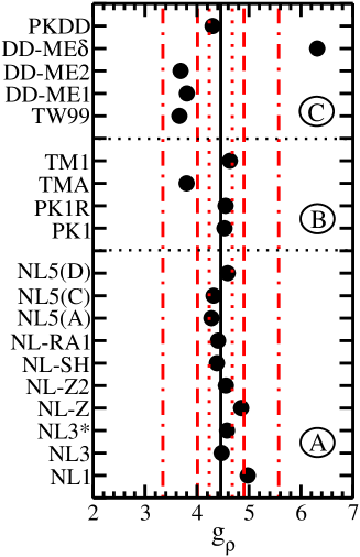
Figure 3: (Color online) The same as Fig. 2 but for the $g_{\rho}$ parameter. Red dotted, dashed and dash-dotted lines show the $\pm 5$%, $\pm 10$% and $\pm 25$% deviation bands with respect of mean values.

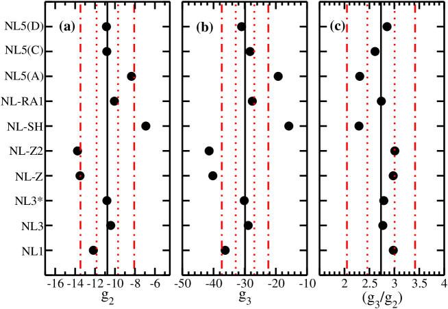
Figure 4: (Color online) The same as Fig. 2 but for the $g_{2}$ and $g_{3}$ parameters. Red dotted and dash-dotted lines show the $\pm 10$% and $\pm 25$% deviation bands with respect of the mean values. Note that only the functionals which belong to group A are considered here.

The 2-dimensional distributions of the parameters of the acceptable functional variations for the NL5(C) CEDF are presented in Fig. 5. The parameters vary with respect of the central value of the distribution (which are typically given by the parameters of optimum functional) by at most 1.5% for $m_{\sigma}$, 3% for $g_{\sigma}$, 3% for $g_{\omega}$, 3% for $g_{\rho}$, 7% for $g_{2}$ and 10% for $g_{3}$. However, these ranges of the parameter variations are dependent on the details of the fitting protocol. For example, in the NL5(A) functional these ranges of the parameter variations are substantially larger for the $g_{2}$ and $g_{3}$ parameters for which they are around 20% and 40%, respectively (see Fig. 6a). These larger ranges for the $g_{2}$ and $g_{3}$ parameters in the acceptable NL5(A) functionals as compared with the NL5(C) ones are the consequence of the 4-fold increase of adopted error for $K_{0}$ (from 2.5% up to 10% [see Table 1]).

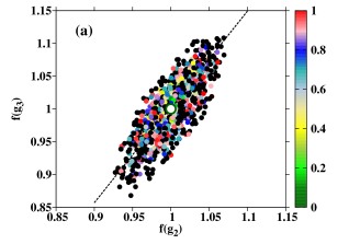
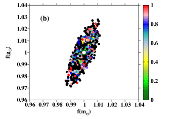
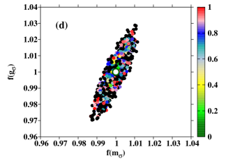
Figure 5: (Color online) Two-dimensional projections of the distribution of the functional variations in the 6-dimensional parameter hyperspace. The colors indicate the $a$ value of the $\chi^{2}_{norm}({\bf p})$ of the functional variation where the latter is expressed as $\chi^{2}_{norm}({\bf p})=\chi^{2}_{norm}({\bf p}_{0})+a$. The colormap is used for the functional variations with $a\leq 1.0$; there are 500 such variations. Note that it was found in the studies that further increase of the number of functional variations does not change the results for statistical errors. In addition, black circles are used for the functionals with $1.0<a\leq 1.25$. The optimum functional is shown by large open symbol. The dashed line in panel (a) shows the parametric correlations between $g_{2}$ and $g_{3}$ parameters defined by Eq. (10).

The analysis of these distributions can also provide the information on the presence of non-linear effects which are related either to non-linear dependencies of the observables on the coupling constants or complicated structure of the $\chi^{2}$ hypersurface exibiting several separated local minima Bürvenich et al. (2004). The position of the optimum functional in the plots of Figs. 5 and 6 corresponds to the crossing point of the $f(par_{i})=1.0$ and $f(par_{j})=1.0$ lines. In absolute majority of the cases the distributions shown in Figs. 5 and 6 have ellipsoid-like shapes with central point of the distribution at this crossing point. This means that non-linear effects are not affecting these distributions. The only exception is the case of the $f(g_{3})-f(g_{2})$ distribution for the NL5(A) functional in which the optimum functional is located off the center of the distribution (see Fig. 6a).

In addition, the correlations between the parameters of the functional can be easily defined from these distributions. Strong correlations between the $m_{\sigma}$ and $g_{\sigma}$ parameters are clearly visible in Figs. 5d and 6d. The same is true for the pair of the $m_{\sigma}$ and $g_{\omega}$ parameters (see Figs. 5b and 6b). This is not surprising since these parameters enter the definition of the nucleonic potential via the sum of attractive scalar potential $S$ (which depends on $m_{\sigma}$ and $g_{\sigma}$) and repulsive vector potential $V$ (which depends on $m_{\omega}$ and $g_{\sigma}$) Vretenar et al. (2005). Note that $m_{\omega}$ is fixed at $m_{\omega}=782.6$ MeV (see Table 2). It is interesting to mention that these strong correlations between the $m_{\sigma}$ and $g_{\omega}$ parameters are clearly visible in Figs. 1a, b, d, and e where the modifications of the factors $f(g_{\omega})$ and $f(m_{\sigma})$ lead to almost the same changes in binding energies and charge radii.

In contrast, the $g_{\rho}$ parameter does not correlate with other parameters of the functional. This is illustrated in Figs. 5c and 6c where the $f(g_{\rho})-f(m_{\sigma})$ distributions are plotted. The fact of the absence of the correlations are easy to understand since the $g_{\rho}$ parameter defines the isovector properties of the functionals while the $m_{\sigma}$ parameter the attractive scalar potential $S$.

The parametric correlations are especially pronounced for the $g_{2}$ and $g_{3}$ parameters which define the density dependence of the functional via a non-linear meson coupling (see Eq. (8)). Figs. 5a and 6a clearly show that these two parameters are not independent and that the following linear dependence

$$f(g_{3})=af(g_{2})+b$$ (10)

exists. The parameters $a$ and $b$, defined from $f(g_{3})-f(g_{2})$ distributions shown in Figs. 5a and 6a, have the following values $a=1.461276$ and $b=-0.458276$ for NL5(C) and $a=1.643$ and $b=-0.64693$ for NL5(A). These parametric correlations are more pronounced for the NL5(A) functional for which the $f(g_{3})-f(g_{2})$ distribution is narrower and more elongated.

The NL5() functionals depends on 6 parameters. The present analysis strongly suggests that its parameter dependence could be reduced to 5 independent parameters, namely, $m_{\sigma}$, $g_{\sigma}$, $g_{\omega}$, $g_{\rho}$, and $g_{2}$ if the parametric correlations given in Eq. (10) are taken into account. However, this requires new refit of the functional with linear dependence of Eq. (10) explicitly used in the fitting protocol. An alternative analysis in manifold boundary approximation method (Ref. Nikšić et al. (2017)) has shown that it is possible to reduce the dimension of the parameter hyperspace of the DD-PC1 CEDF from ten parameters to eight without sacrificing the quality of the reproduction of experimental and empirical data. Similar to the NL5() case, this reduction in Ref. Nikšić et al. (2017) takes place in the channel of the functional which defines its density dependence. In the context of the analysis of theoretical uncertainties there is one clear advantage of the reduction of the dimensionality of the parameter hyperspace via the removal of parametric correlations: such reduction leads to the decrease of statistical errors. This was illustrated in Ref. Debes and Dudek (2017) on the example of the study of statistical errors in the single-particle energies and it is discussed for ground state observables in the present manuscript in Sec. V.2.

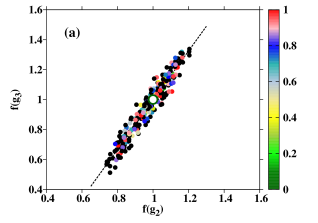
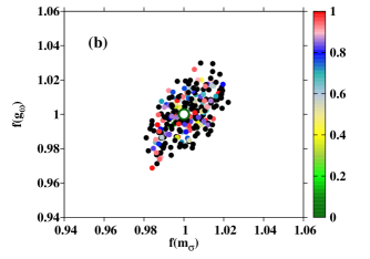
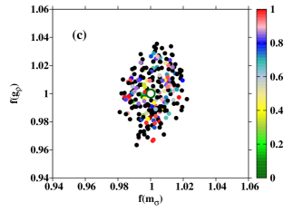
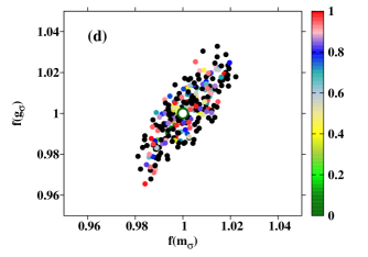
Figure 6: (Color online) The same as Fig. 5 but for the NL5(A) functional. Considering the increase of the size of the parameter hyperspace and extremely time-consuming nature of numerical calculations only 150 functional variations satisfying the condition of Eq. (4) have been collected. This leads to some reduction of the accuracy of the calculations of statistical errors. However, the analysis of the NL5(C) results for which 500 acceptable functional variations have been collected allows to conclude that statistical errors obtained with the 150 functional variations differ from those calculated with 500 variations only by approximately 5%.

V Statistical errors in the ground state observables of even-even nuclei.

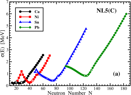
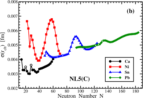
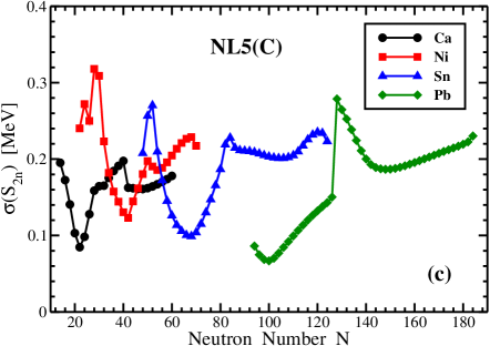
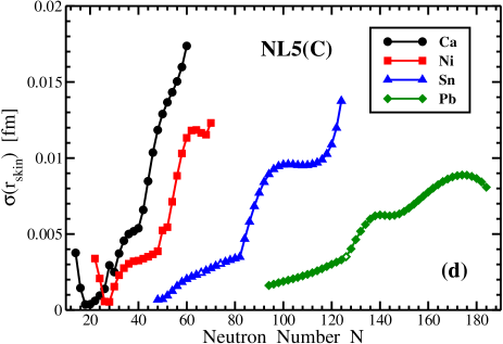
Figure 7: (Color online) The propagation of statistical errors in binding energies [panel (a)], charge radii [panel (b)], two-neutron separation energies [panel (c)] and neutron skins [panel (d)] with neutron number. The results are presented for the Ca ($Z=20$), Ni ($Z=28$), Sn ($Z=50$) and Pb ($Z=82$) isotopes between two-proton and two-neutron drip lines. Open symbols are used to indicate the nuclei whose experimental data of the type shown on the vertical axis of the panel has been used in the fitting protocol of the NL5(C) functional.

V.1 The case of the NL5(C) functional

In this section we will investigate statistical errors in the description of the ground state properties of spherical Ca, Ni, Sn and Pb even-even isotopes. Within the isotope chain the calculations cover all nuclei between the two-proton and two-neutron drip lines. When possible the statistical errors obtained in the present study will be compared with systematic uncertainties defined in Refs. Agbemava et al. (2014); Afanasjev and Agbemava (2016). In addition, they will be compared with statistical errors obtained in the Skyrme DFT study with UNEDF0 functional of Ref. Gao et al. (2013).

Statistical errors in binding energies obtained with the CEDF NL5(C) and their propagation with the neutron number are shown in Fig. 7a. They are close to adopted errors of the fitting protocol [0.1% of binding energy (see Table 1)] for the nuclei used in the fit. With increasing isospin the statistical errors in binding energies substantially increase reaching $\sim 2.6$, $\sim 2.6$, $\sim 5.0$ and $\sim 6.0$ MeV at the two-neutron drip line in the Ca, Ni, Sn and Pb isotope chains, respectively. However, they are significantly smaller at the neutron-drip line than those obtained in the Skyrme DFT studies of Ref. Gao et al. (2013); by factors 4.6, 3.1, 3.4 and 2.3 for the Ca, Ni, Sn and Pb isotopes, respectively. Statistical errors in binding energies of these nuclei are by a factor 2-3 smaller than systematic uncertainties in the binding energies obtained in Ref. Agbemava et al. (2014) (see Fig. 8 in this reference). Note that the estimate of systematic uncertainties of Ref. Agbemava et al. (2014) are based only on four CEDFs, namely, NL3*, DD-PC1, DD-ME2 and DD-ME$\delta$. The investigation of Ref. Afanasjev et al. (2015) suggests that the addition of the PC-PK1 functional could lead to a substantial increase of systematic uncertainties in binding energies. This is at least a case for the Yb ($Z=70$) isotopes for which they increase by a factor of 2.1 when the PC-PK1 results are added (see Fig. 3 in Ref. Afanasjev and Agbemava (2016)).

Statistical errors in charge radii $r_{ch}$ are presented in Fig. 7b. They are in the vicinity of 0.1% of the calculated $r_{ch}$ values shown in Fig. 23 of Ref. Agbemava et al. (2014). For the nuclei used in the fitting protocol, statistical errors are below the adopted errors of 0.2% for $r_{ch}$. Calculated statistical errors are below 25% of the rms deviations $\Delta r_{ch}^{rms}$ between calculated and experimental charge radii, which are typical for the state-of-the-art CEDFs and which are shown in Table VI of Ref. Agbemava et al. (2014). Systematic uncertainties in the predictions of charge radii of the Ca and Ni isotopes obtained from the set of the four functionals (see Fig. 24 of Ref. Agbemava et al. (2014)) are substantially larger (on average, by an approximate factor of 8 and 10, respectively) than relevant statistical errors. This difference goes down with the increase of proton number. For example, the situation in the Pb isotopes depends on the neutron number $N$. Statistical errors are only somewhat smaller than systematic uncertainties in the Pb nuclei with $N\sim 110$ and $N\sim 126$. On the other hand, they are smaller than statistical uncertainties by a factor of approximately 10 for the nuclei with $N\sim 102$. On average, for the Pb nuclei the statistical errors in charge radii are by a factor of approximately 4 smaller than relevant systematic uncertainties. Similar situation is observed also in the Sn isotopes, but the average difference between statistical errors and statistical uncertainties in charge radii is of the order of 7.

Contrary to Skyrme DFT calculations with the UNEDF0 functional (see Fig. 4b in Ref. Gao et al. (2013)), statistical errors in charge radii calculated with NL5(C) (see Fig. 7b in the present paper) do not show significant increase with neutron number. In reality, the $\sigma(r_{ch})$ values obtained with NL5(C) for the Sn and Pb isotopes show very modest increase of approximately 20% on going from two-proton to two-neutron drip line. Note that the $\sigma(r_{ch})$ values show some fluctuations as a function of neutron number which are due to underlying shell structure; they become especially pronounced in the Ni isotopes. While statistical errors for charge radii of the Ca, Ni and Sn isotopes are comparable for Skyrme UNEDF0 and CDFT NL5(C) calculations for the nuclei near two-proton drip line, the situation changes drastically with the increase of neutron number so that for the Ca, Ni, Sn and Pb nuclei at the two-neutron drip line the $\sigma(r_{ch})$ values obtained in Skyrme calculations are by factor of 17-33 larger than those obtained in CDFT calculations with CEDF NL5(C).

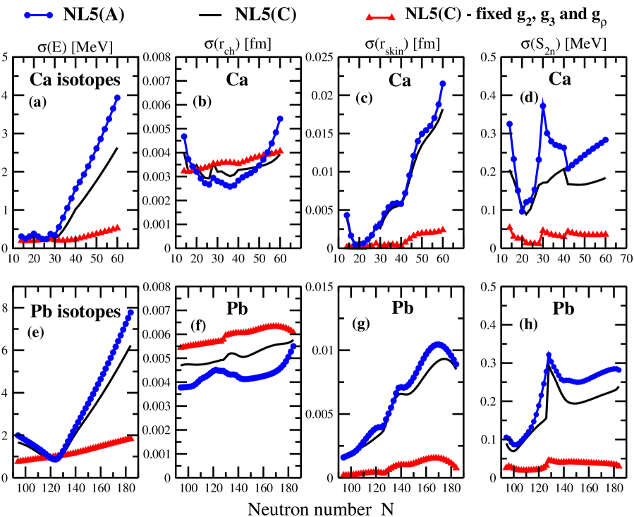
Figure 8: (Color online) The propagation of statistical errors for the binding energies $(\sigma(E))$, charge radii $(\sigma(r_{ch}))$, neutron skins $(\sigma(r_{skin}))$ and two-neutron separation energies $(\sigma(S_{2n}))$ in the Ca and Pb isotope chains. The results of the calculations with the NL5(C) and NL5(A) functionals are shown by solid black line and blue solid line with solid circles, respectively. In addition, red triangle symbols show statistical errors for the NL5(C) functional under the condition that the $g_{\rho}$, $g_{2}$ and $g_{3}$ parameters are fixed at the values corresponding to optimum NL5(C) functional.

Statistical errors in two-neutron separation energies are displayed in Fig. 7c. They are typically in the range of 0.1 - 0.3 MeV and do not show a clear tendency of the increase on approaching two-neutron drip line. These statistical errors show substantial fluctuations as a function of neutron number with the changes in the slope of $\sigma(S_{2n})$ typically taking place in the vicinity of the shell ($N=20,28,50,82$ and 126) and subshell ($N=40$) closures. The calculated $\sigma(S_{2n})$ values are typically by a factor of 3-4 smaller than the rms-deviations between theory and experiment for the state-of-the-art CEDF (see Table III in Ref. Agbemava et al. (2014)). It is interesting to compare our results with the ones obtained in Skyrme DFT calculations of Ref. Gao et al. (2013). While the $\sigma(S_{2n})$ values are comparable for both models in the vicinity of the $\beta$-stability line, they increase drastically with increasing neutron number in the Skyrme DFT calculations approaching $\sim 1.4$, $\sim 1.4$, $\sim 0.8$ and $\sim 0.75$ MeV for Ca, Ni, Sn and Pb nuclei at the two-neutron drip line, respectively. This trend is contrary to the one seen in the CDFT results.

Statistical errors in the neutron skin thickness $r_{skin}$ are shown in Fig. 7d. They are close to zero near the $N=Z$ line but increase with increasing neutron number. This increase is rapid in the Ca, Ni and Sn isotopes but it is more moderate in the Pb isotopes. An interesting feature of the latter chain is the decrease of the $\sigma(r_{skin})$ values above $N\sim 170$ which is most likely due to underlying shell effects. The statistical errors in the neutron skin thickness are substantially larger in the Skyrme DFT calculations with the UNEDF0 and SV-min functionals (Ref. Kortelainen et al. (2013)) than in the present RHB calculations with CEDF NL5(C). For example, for ²⁰⁸Pb the $\sigma(r_{skin})$ values are 0.058 fm, 0.037 fm and 0.0035 fm in the calculations with the UNEDF0, SV-min and NL5(C) functionals, respectively. In the neutron-rich Ca isotopes near the two-neutron drip line the $\sigma(r_{skin})$ values obtained in non-relativistic calculations are by a factor of approximately 7 larger than those obtained in the relativistic ones. The statistical errors in the neutron skin thickness shown in Fig. 7d are substantially smaller than systematic uncertainties shown in Fig. 25 of Ref. Agbemava et al. (2014). In the vicinity of the two-neutron drip line, the latter ones reach 0.15 fm, 0.2 fm, 0.25 fm and 0.25 fm in the neutron rich Ca, Ni, Sn and Pb nuclei, respectively.

V.2 The impact of the details of the fitting protocol and of soft parameters on statistical errors.

It is important to understand how the details of the fitting protocol could affect the statistical errors in physical observables of interest. Considering the ingredients entering into fitting protocol and the uncertainties in the definition of empirical/experimental values of physical observables and adopted errors, the complete answer to this question requires enormous amount of numerical calculations which are beyond the scope of the present investigation. However, in order to get a crude estimate of potential changes in statistical errors additional calculations have been performed for the two cases discussed below.

In the first case, we analyse statistical errors obtained with the NL5(A) functional. This functional differs from the NL5(C) one by an increased adopted error for $K_{0}$ and the presence of neutron skin of ⁹⁰Zr in the fitting protocol (see Table 1). As a consequence of these features, the acceptable NL5(A) functionals show larger range of variations for the $g_{2}$ and $g_{3}$ parameters as compared with the NL5(C) ones (compare Figs. 5a and 6a). This leads to some increase in statistical errors for binding energies (especially in neutron-rich nuclei in which the $\sigma(E)$ values are increased by $\sim 30\%$ as compared with the NL5(C) results) and two-neutron separation energies (see Figs. 8a, e, d and h). On the contrary, as compared with the NL5(C) results statistical errors in neutron skin are only slightly increased (see Fig. 8c and g) and statistical errors in charge radii even decrease in the Pb isotopes and for some Ca isotopes (see Fig. 8b and f).

Despite these changes statistical errors for physical observables of interest obtained with the NL5(A) functional still remain substantially smaller than those obtained in Skyrme DFT calculations (compare results presented in this subsection with the discussion in Sec. V.1).

In the second case, we use the NL5(C) functional but fix the $g_{2}$, $g_{3}$ and $g_{\rho}$ parameters at the values of the optimal functional during the Monte-Carlo procedure. As shown in Secs. III and IV, the $g_{\sigma}$, $m_{\sigma}$ and $g_{\omega}$ parameters, which are allowed to change during Monte-Carlo procedure, are well localized in the parameter hyperspace and they vary in a very narrow range with respect of the optimum functional. Fig. 8 compares the results for the Ca and Pb nuclei presented in Fig. 7 with statistical errors obtained in such calculations. The freezing of the $g_{2}$, $g_{3}$ and $g_{\rho}$ parameters in the functional leads to a substantial decrease of statistical errors in binding energies of neutron-rich nuclei so that in two-neutron drip line nuclei they are only by a factor of approximately two larger than those for the nuclei used in the fitting protocol (Fig. 8a and e). Note that the $\sigma(E)$ values obtained is such calculations are typically significanly smaller (especially in very neutron-rich nuclei) than those obtained in full NL5(C) calculations shown by solid black line. The only exception is the region of neutron numbers in which the experimental data on binding energies was used in the fitting protocol. Statistical errors in two-neutron separation energies become very small ($\sigma(S_{2n})<0.05$ MeV) in the calculations with fixed $g_{2}$, $g_{3}$ and $g_{\rho}$ parameters (see Fig. 8d and h). They are also significantly smaller than those obtained in full NL5(C) calculations. Simultaneous freezing of the $g_{2}$, $g_{3}$ and $g_{\rho}$ parameters leads to a substantial decrease of statistical errors in neutron skin so that in the most of the nuclei they are very close to zero (see Fig. 8c and g). On the contrary, the impact of freezing of the $g_{2}$, $g_{3}$ and $g_{\rho}$ parameters on statistical errors in charge radii is very limited (see Fig. 8b and f)). It is interesting that it leads to slight increase of the $\sigma(r_{ch})$ as compared with those obtained in full NL5(C) calculations.

This analysis clearly illustrates the importance of the discrimination of the impact of the stiff and soft parameters of CEDFs on statistical errors. Such a separation of the parameters into two types was discussed in Ref. Nikšić et al. (2017). Even when the parameters of nuclear EDFs are adjusted to experimental/empirical/pseudo data, their predictions are sensitive to only a few combinations of parameters (stiff parameter combinations) and exhibit an exponential decrease of sensitivity to variations of the remaining soft parameters that are only approximately constrained by data. In non-linear meson coupling models, the stiff parameters are represented by $m_{\omega}$, $g_{\omega}$ and $g_{\sigma}$. Their contribution to statistical errors is rather small and mostly independent of neutron number. On the contrary, the combination of soft parameters $g_{2}$, $g_{3}$ and $g_{\rho}$ leads to a significant increase of statistical errors for binding energies and neutron skins on approaching two-neutron drip line. They also lead to an increase of statistical errors in two-neutron separation energies. Thus, one can conclude that the presence of soft parameters in the CEDFs is the major source of statistical errors.

VI Statistical errors in the single-particle energies

Table 4: Neutron and proton single-particle states in the ²⁰⁸Pb nucleus. Columns 2 and 5 show the mean energies $\bar{e}_{i}$ [in MeV] of these states obtained in the calculations with CEDF NL5(C). Columns 3 and 6 show their standard deviations $\sigma(e_{i})$ [in MeV]. The positions of the proton and neutron Fermi levels are indicated.

Neutron			Proton
Orbital	$\bar{e}_{\nu}$	$\sigma(e_{\nu})$	Orbital	$\bar{e}_{\pi}$	$\sigma(e_{\pi})$
1	2	3	4	5	6
1$s_{1/2}$	-58.257	0.424	1$s_{1/2}$	-47.100	0.401
1$p_{3/2}$	-52.142	0.376	1$p_{3/2}$	-41.573	0.360
1$p_{1/2}$	-51.581	0.363	1$p_{1/2}$	-40.933	0.345
1$d_{5/2}$	-44.809	0.316	1$d_{5/2}$	-34.691	0.307
1$d_{3/2}$	-43.497	0.282	1$d_{3/2}$	-33.249	0.270
2$s_{1/2}$	-40.566	0.241	2$s_{1/2}$	-29.725	0.221
1$f_{7/2}$	-36.614	0.252	1$f_{7/2}$	-26.864	0.251
1$f_{5/2}$	-34.228	0.189	1$f_{5/2}$	-24.320	0.187
2$p_{3/2}$	-30.515	0.149	2$p_{3/2}$	-20.045	0.150
2$p_{1/2}$	-29.526	0.128	2$p_{1/2}$	-19.054	0.136
1$g_{9/2}$	-27.862	0.191	1$g_{9/2}$	-18.402	0.199
1$g_{7/2}$	-24.177	0.112	1$g_{7/2}$	-14.556	0.128
2$d_{5/2}$	-20.708	0.098	2$d_{5/2}$	-10.465	0.122
2$d_{3/2}$	-19.127	0.091	1$h_{11/2}$	-9.544	0.159
1$h_{11/2}$	-18.809	0.141	2$d_{3/2}$	-8.903	0.121
3$s_{1/2}$	-18.301	0.095	3$s_{1/2}$	-7.729	0.121
			Proton Fermi level
1$h_{9/2}$	-13.774	0.108	1$h_{9/2}$	-4.367	0.134
2$f_{7/2}$	-11.320	0.085	2$f_{7/2}$	-1.107	0.120
1$i_{13/2}$	-9.661	0.104	1$i_{13/2}$	-0.481	0.133
2$f_{5/2}$	-9.390	0.098	2$f_{5/2}$	0.802	0.131
3$p_{3/2}$	-8.591	0.087	3$p_{3/2}$	2.133	0.121
3$p_{1/2}$	-7.895	0.090	3$p_{1/2}$	2.828	0.125
Neutron Fermi level
1$i_{11/2}$	-3.515	0.148
2$g_{9/2}$	-2.688	0.080
3$d_{5/2}$	-0.873	0.062
2$g_{7/2}$	-0.855	0.090
4$s_{1/2}$	-0.599	0.050
1$j_{15/2}$	-0.597	0.081
3$d_{3/2}$	-0.281	0.061
4$p_{3/2}$	2.557	0.018
4$p_{1/2}$	2.669	0.019

Table 5: The same as Table 4 but for the ²⁶⁶Pb nucleus. The states in the energy range from $\sim-42$ MeV up to $\sim-20$ MeV are omitted in order to simplify the table.

Neutron			Proton
Orbital	$\bar{e}_{\nu}$	$\sigma(e_{\nu})$	Orbital	$\bar{e}_{\pi}$	$\sigma(e_{\pi})$
1	2	3	4	5	6
1$s_{1/2}$	-53.045	0.364	1$s_{1/2}$	-49.945	0.323
1$p_{3/2}$	-47.922	0.333	1$p_{3/2}$	-45.498	0.304
1$p_{1/2}$	-47.567	0.326	1$p_{1/2}$	-45.070	0.297
—–	—–	—–	—–	——	—–
2$d_{3/2}$	-20.427	0.153	1$h_{11/2}$	-18.396	0.199
3$s_{1/2}$	-19.619	0.153	2$d_{3/2}$	-18.075	0.176
1$h_{11/2}$	-19.595	0.188	3$s_{1/2}$	-16.727	0.169
			Proton Fermi level
1$h_{9/2}$	-16.052	0.159	1$h_{9/2}$	-14.726	0.186
2$f_{7/2}$	-13.384	0.142	2$f_{7/2}$	-10.867	0.172
2$f_{5/2}$	-11.882	0.138	1$i_{13/2}$	-10.415	0.184
1$i_{13/2}$	-11.638	0.163	2$f_{5/2}$	-9.372	0.182
3$p_{3/2}$	-11.057	0.130	3$p_{3/2}$	-7.655	0.171
3$p_{1/2}$	-10.494	0.128	3$p_{1/2}$	-7.086	0.177
1$i_{11/2}$	-7.153	0.161	1$i_{11/2}$	-5.779	0.198
2$g_{9/2}$	-5.728	0.124	2$g_{9/2}$	-2.583	0.174
2$g_{7/2}$	-4.138	0.123	1$j_{15/2}$	-2.234	0.175
3$d_{5/2}$	-3.847	0.100	2$g_{7/2}$	-0.896	0.186
1$j_{15/2}$	-3.691	0.143	3$d_{5/2}$	0.851	0.168
4$s_{1/2}$	-3.342	0.088	3$d_{3/2}$	1.540	0.173
3$d_{3/2}$	-3.252	0.097	4$s_{1/2}$	2.130	0.162
Neutron Fermi level
2$h_{11/2}$	1.038	0.096	1$j_{13/2}$	3.185	0.216
4$p_{3/2}$	1.292	0.034
1$j_{13/2}$	1.406	0.164
4$p_{1/2}$	1.460	0.033
3$f_{7/2}$	1.546	0.051
3$f_{5/2}$	1.998	0.045
2$h_{9/2}$	2.387	0.086

The energies of the single-particle states $e_{i}$ represent another quantity which affects many physical observables (see Refs. Litvinova and Afanasjev (2011); Afanasjev and Litvinova (2015); Afanasjev and Shawaqfeh (2011); Afanasjev et al. (2015); Agbemava et al. (2015)). In this section we investigate statistical errors in the description of the energies of the single-particle states $e_{i}$; they are quantified by the standard deviations $\sigma(e_{i})$. We focus on three nuclei, namely, ²⁰⁸Pb, ²⁶⁶Pb and ³⁰⁴120. The first one is well known doubly magic nucleus which serves as a testing ground in many theoretical studies. Second nucleus is the last bound neutron-rich Pb isotope in absolute majority of theoretical studies (see Fig. 14 in Ref. Agbemava et al. (2014)); it is characterized by large $N=184$ shell gap (see Fig. 6a in Ref. Afanasjev et al. (2015)). Third nucleus is the $Z=120,N=184$ superheavy nucleus which is considered as doubly magic in a number of studies (see, for example, Ref. Bender et al. (1999)); this conclusion is however model dependent (see Refs. Bender et al. (1999, 2001); Afanasjev et al. (2003); Agbemava et al. (2015) and references quoted therein). The comparison of the results obtained for these three nuclei will allow to assess the propagation of statistical errors on going from the valley of beta-stability towards the extremes of neutron number and charge.

Table 6: The same as Table 4 but for the ³⁰⁴120 nucleus. Neutron states in the energy range from $\sim-50$ MeV up to $\sim-25$ MeV and proton states in the energy range from $\sim-35$ MeV up to $\sim-12$ MeV are omitted in order to simplify the table.

Neutron			Proton
Orbital	$\bar{e}_{\nu}$	$\sigma(e_{\nu})$	Orbital	$\bar{e}_{\pi}$	$\sigma(e_{\pi})$
1	2	3	4	5	6
1$s_{1/2}$	-57.748	0.386	1$s_{1/2}$	-41.480	0.367
1$p_{3/2}$	-53.698	0.362	1$p_{3/2}$	-37.545	0.349
1$p_{1/2}$	-53.459	0.359	1$p_{1/2}$	-37.246	0.343
—–	—–	—–	—–	——	—–
3$s_{1/2}$	-24.421	0.107	3$s_{1/2}$	-9.349	0.134
1$h_{9/2}$	-23.315	0.105	1$h_{9/2}$	-8.169	0.126
2$f_{7/2}$	-19.452	0.098	1$i_{13/2}$	-4.150	0.153
1$i_{13/2}$	-18.893	0.132	2$f_{7/2}$	-3.903	0.123
2$f_{5/2}$	-17.953	0.092	2$f_{5/2}$	-2.418	0.121
			Proton Fermi level
3$p_{3/2}$	-15.293	0.092	3$p_{3/2}$	-0.302	0.132
3$p_{1/2}$	-14.947	0.093	3$p_{1/2}$	0.017	0.134
1$i_{11/2}$	-14.288	0.103	1$i_{11/2}$	0.612	0.130
2$g_{9/2}$	-11.194	0.086	1$j_{15/2}$	3.758	0.133
1$j_{15/2}$	-10.809	0.103	2$g_{9/2}$	4.230	0.119
2$g_{7/2}$	-9.206	0.099
3$d_{5/2}$	-7.336	0.085
3$d_{3/2}$	-7.014	0.085
4$s_{1/2}$	-6.372	0.077
Neutron Fermi level
1$j_{13/2}$	-5.195	0.136
2$h_{11/2}$	-3.278	0.084
1$k_{17/2}$	-2.669	0.084
2$h_{9/2}$	-1.227	0.100
3$f_{7/2}$	-0.626	0.066
3$f_{5/2}$	-0.188	0.067
4$p_{3/2}$	0.080	0.051
4$p_{1/2}$	0.259	0.052
5$s_{1/2}$	2.353	0.016
4$d_{5/2}$	2.822	0.017

Tables 4, 5 and 6 show the calculated mean energies $\bar{e}_{i}$ of the single-particle states and related standard deviations $\sigma(e_{i})$ obtained in these nuclei. The general trend, which is clearly seen in these tables, is the decrease of statistical errors on going from the bottom of nucleonic potential towards continuum. The states at the bottom of potential are characterized by $\sigma(e_{i})\sim 0.35$ MeV both for proton and neutron subsystems for all nuclei under consideration. In ²⁰⁸Pb, the neutron and proton states are characterized by $\sigma(e_{i})\sim 0.1$ MeV in the vicinity of the respective Fermi levels which have similar energies. The addition of neutrons leading to ²⁶⁶Pb moves the proton Fermi level to lower energies (deeper into the potential) and neutron Fermi level closer to continuum limit. As a consequence, the $\sigma(e_{i})$ values for the proton states in the vicinity of the proton Fermi level increase to $\sim 0.15$ MeV (see Table 5). On the contrary, with the exception of the high-$j$ $\nu 1j_{15/2}$ and $\nu 1j_{13/2}$ states for which $\sigma(e_{i})\sim 0.15$ MeV, the $\sigma(e_{i})$ values for the neutron states in the vicinity of the neutron Fermi level is less than 0.1 MeV (see Table 5). Because the neutron and proton Fermi levels are located at $\sim-6.4$ MeV and $\sim-2.4$ MeV, respectively, in the ¹⁸⁴120 nucleus [which is not far away from their values in ²⁰⁸Pb], the $\sigma(e_{i})$ values for the single-particle states in this nucleus are comparable with the ones in ²⁰⁸Pb (compare tables 4 and 6).

Table 7: Relative energies ${\Delta e}_{i}(m,j)=e_{i}(m)-e_{i}(j)$ of the pairs of neutron ($i=\nu$) and proton ($i=\pi$) single-particle states in the ²⁰⁸Pb nucleus. The pairs of neighboring states $m$ and $j$ shown in the columns 1 and 4 are defined from the single-particle spectra obtained with the NL5(C) CEDF. The columns 2 and 5 show their mean relative energies $\overline{\Delta e}_{i}(m,j)$ [in MeV] while the columns 3 and 6 show standard deviations $\sigma(\Delta e_{i}(m,j))$ [in MeV]. All the pairs of the states up to the label “proton/neutron Fermi level” have both members located below respective Fermi levels. Next line after this statement indicates the pair of the states one of the members of which is located below the large shell gap (either proton $Z=82$ or neutron $N=126$ one) and another above this gap. Subsequent lines show the pairs of the states both members of which are located above respective Fermi levels (above proton $Z=82$ or neutron $N=126$ shell gaps).

Neutron			Proton
Orbital			Orbital
pairs $(m,j)$	$\overline{\Delta e}_{\nu}$	$\sigma(\Delta e_{\nu})$	pairs $(m,j)$	$\overline{\Delta e}_{\pi}$	$\sigma(\Delta e_{\pi})$
1	2	3	4	5	6
1$s_{1/2}$ - 1$p_{3/2}$	6.115	0.054	1$s_{1/2}$ - 1$p_{3/2}$	5.527	0.049
1$p_{3/2}$ - 1$p_{1/2}$	0.560	0.013	1$p_{3/2}$ - 1$p_{1/2}$	0.640	0.016
1$p_{1/2}$ - 1$d_{5/2}$	6.772	0.053	1$p_{1/2}$ - 1$d_{5/2}$	6.242	0.045
1$d_{5/2}$ - 1$d_{3/2}$	1.313	0.037	1$d_{5/2}$ - 1$d_{3/2}$	1.442	0.042
1$d_{3/2}$ - 2$s_{1/2}$	2.931	0.047	1$d_{3/2}$ - 2$s_{1/2}$	3.524	0.058
2$s_{1/2}$ - 1$f_{7/2}$	3.951	0.033	2$s_{1/2}$ - 1$f_{7/2}$	2.860	0.049
1$f_{7/2}$ - 1$f_{5/2}$	2.386	0.073	1$f_{7/2}$ - 1$f_{5/2}$	2.545	0.079
1$f_{5/2}$ - 2$p_{3/2}$	3.713	0.055	1$f_{5/2}$ - 2$p_{3/2}$	4.274	0.063
2$p_{3/2}$ - 2$p_{1/2}$	0.989	0.028	2$p_{3/2}$ - 2$p_{1/2}$	0.991	0.028
2$p_{1/2}$ - 1$g_{9/2}$	1.664	0.090	2$p_{1/2}$ - 1$g_{9/2}$	0.652	0.106
1$g_{9/2}$ - 1$g_{7/2}$	3.685	0.116	1$g_{9/2}$ - 1$g_{7/2}$	3.846	0.121
1$g_{7/2}$ - 2$d_{5/2}$	3.469	0.051	1$g_{7/2}$ - 2$d_{5/2}$	4.092	0.058
2$d_{5/2}$ - 2$d_{3/2}$	1.581	0.039	2$d_{5/2}$ - 1$h_{11/2}$	0.920	0.098
2$d_{3/2}$ - 1$h_{11/2}$	0.318	0.122	1$h_{11/2}$ - 2$d_{3/2}$	0.641	0.133
1$h_{11/2}$ - 3$s_{1/2}$	0.507	0.113	2$d_{3/2}$ - 3$s_{1/2}$	1.174	0.025
			below proton Fermi level
3$s_{1/2}$ - 1$h_{9/2}$	4.527	0.094	3$s_{1/2}$ - 1$h_{9/2}$	3.362	0.095
1$h_{9/2}$ - 2$f_{7/2}$	2.455	0.078	1$h_{9/2}$ - 2$f_{7/2}$	3.260	0.081
2$f_{7/2}$ - 1$i_{13/2}$	1.659	0.094	2$f_{7/2}$ - 1$i_{13/2}$	0.626	0.103
1$i_{13/2}$ - 2$f_{5/2}$	0.271	0.128	1$i_{13/2}$ - 2$f_{5/2}$	1.283	0.136
2$f_{5/2}$ - 3$p_{3/2}$	0.799	0.033	2$f_{5/2}$ - 3$p_{3/2}$	1.331	0.031
3$p_{3/2}$ - 3$p_{1/2}$	0.696	0.017	3$p_{3/2}$ - 3$p_{1/2}$	0.695	0.016
below neutron Fermi level
3$p_{1/2}$ - 1$i_{11/2}$	4.380	0.109
1$i_{11/2}$ - 2$g_{9/2}$	0.827	0.118
2$g_{9/2}$ - 3$d_{5/2}$	1.816	0.022
3$d_{5/2}$ - 2$g_{7/2}$	0.018	0.036
2$g_{7/2}$ - 4$s_{1/2}$	0.256	0.044
4$s_{1/2}$ - 1$j_{15/2}$	0.003	0.084
1$j_{15/2}$ - 3$d_{3/2}$	0.316	0.090
3$d_{3/2}$ - 4$p_{3/2}$	2.837	0.044
4$p_{3/2}$ - 4$p_{1/2}$	0.113	0.003

The detailed analysis of the results of the calculations shows that the freedom to rebalance the depths of the proton and neutron potentials is a major source of these statistical errors in the energies of the single-particle states. Indeed, it was observed that when proton potential becomes deeper as compared with the one in the optimum functional, the neutron potential becomes less deep as compared with the one in optimum functional. This leads to more/less bound proton/neutron single-particle states and allows to keep total energy of the system close to the one in the optimum functional. The opposite situation with deeper neutron and less deep proton potentials takes place with similar frequency.

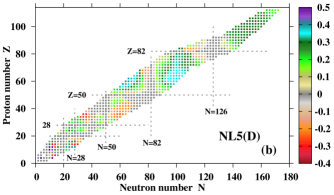
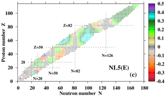
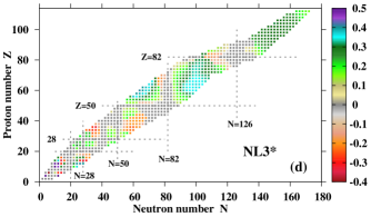
Figure 11: (Color online) Charge quadrupole deformations $\beta_{2}$ of the ground states in even-even nuclei obtained in the RHB calculations with indicated CEDFs.

In general, statistical errors in the absolute energies of the single-particle states could affect model predictions for the position of the two-neutron drip line. Indeed, as discussed in Ref. Afanasjev et al. (2015) its position sensitively depends on the positions (in absolute energy) and the distribution of the single-particle states (and especially high-$j$ intruder and extruder ones) located around the continuum limit. However, in the nuclei around ²⁶⁶Pb the standard deviations $\sigma(e_{i})$ for such neutron single-particle states are safely below 0.1 MeV (see Table 5); the only exception is the $\nu 1j_{13/2}$ orbital for which $\sigma(e_{i})=0.164$ MeV. Thus, it is reasonable to expect that the impact of statistical errors in the energies of the single-particle states on the position of two-neutron drip line will be rather modest. Moreover, these statistical errors are substantially smaller than systematic uncertainties in the predictions of the energies of single-particle states which for many orbitals exceed 1 MeV in nuclei near two-neutron drip line (see Figs. 11c and 6c in Ref. Afanasjev et al. (2015)). These facts suggest that the theoretical uncertainties in the prediction of the position of two-neutron drip line are dominated by systematic ones.

While the accuracy of the prediction of the position of the neutron drip line is sensitive to calculated absolute energies of the single-particle states, the accuracy of the reproduction of the single-particle spectra depends mostly on the predictions of the relative energies of the single-particle states. Tables 7, 8 and 9 show the mean relative energies $\overline{\Delta e}_{i}$ of the pairs of neighboring single-particle states (as defined in the NL5(C) functional) and related standard deviations $\sigma(\Delta e_{i})$. One can see that in all nuclei the $\sigma(\Delta e_{i})$ values are substantially smaller than the $\overline{\Delta e}_{i}$ values. They are also much smaller than the deviations between theory and experiment for one-(quasi)-particle configurations in spherical Litvinova and Afanasjev (2011); Afanasjev (2015); Afanasjev and Litvinova (2015) and deformed Afanasjev and Shawaqfeh (2011); Dobaczewski et al. (2015) nuclei. Here we assume that statistical errors in the description of the energies of deformed single-particle states are similar to spherical ones which is a reasonable assumption considering that deformed states emerge from spherical ones. Thus, one can conclude that systematic uncertainties in the energies of the single-particle states are more important than statistical ones for the predictions of the single-particle spectra.

Table 8: The same as Table 7 but for the ²⁶⁶Pb nucleus. The states in the energy range from $\sim-42$ MeV up to $\sim-20$ MeV are omitted in order to simplify the table.

Neutron			Proton
Orbital			Orbital
pairs $(m,j)$	$\overline{\Delta e}_{\nu}$	$\sigma(\Delta e_{\nu})$	pairs $(m,j)$	$\overline{\Delta e}_{\pi}$	$\sigma(\Delta e_{\pi})$
1	2	3	4	5	6
1$s_{1/2}$ - 1$p_{3/2}$	5.123	0.037	1$s_{1/2}$ - 1$p_{3/2}$	4.447	0.031
1$p_{3/2}$ - 1$p_{1/2}$	0.355	0.008	1$p_{3/2}$ - 1$p_{1/2}$	0.428	0.010
—–	—–	—–	—–	——	—–
2$d_{5/2}$ - 2$d_{3/2}$	1.143	0.029	2$d_{5/2}$ - 1$h_{11/2}$	0.811	0.071
2$d_{3/2}$ - 3$s_{1/2}$	0.807	0.016	1$h_{11/2}$ - 2$d_{3/2}$	0.322	0.096
3$s_{1/2}$ - 1$h_{11/2}$	0.024	0.077	2$d_{3/2}$ - 3$s_{1/2}$	1.348	0.019
			below proton Fermi level
1$h_{11/2}$ - 1$h_{9/2}$	3.543	0.101	3$s_{1/2}$ - 1$h_{9/2}$	2.001	0.063
1$h_{9/2}$ - 2$f_{7/2}$	2.669	0.055	1$h_{9/2}$ - 2$f_{7/2}$	3.859	0.061
2$f_{7/2}$ - 2$f_{5/2}$	1.502	0.034	2$f_{7/2}$ - 1$i_{13/2}$	0.451	0.079
2$f_{5/2}$ - 1$i_{13/2}$	0.244	0.094	1$i_{13/2}$ - 2$f_{5/2}$	1.043	0.108
1$i_{13/2}$ - 3$p_{3/2}$	0.581	0.088	2$f_{5/2}$ - 3$p_{3/2}$	1.717	0.025
3$p_{3/2}$ - 3$p_{1/2}$	0.562	0.014	3$p_{3/2}$ - 3$p_{1/2}$	0.570	0.014
3$p_{1/2}$ - 1$i_{11/2}$	3.342	0.075	3$p_{1/2}$ - 1$i_{11/2}$	1.307	0.074
1$i_{11/2}$ - 2$g_{9/2}$	1.425	0.084	1$i_{11/2}$ - 2$g_{9/2}$	3.196	0.082
2$g_{9/2}$ - 2$g_{7/2}$	1.590	0.031	2$g_{9/2}$ - 1$j_{15/2}$	0.349	0.079
2$g_{7/2}$ - 3$d_{5/2}$	0.291	0.035	1$j_{15/2}$ - 2$g_{7/2}$	1.338	0.105
3$d_{5/2}$ - 1$j_{15/2}$	0.156	0.085	2$g_{7/2}$ - 3$d_{5/2}$	1.748	0.034
1$j_{15/2}$ - 4$s_{1/2}$	0.349	0.093	3$d_{5/2}$ - 3$d_{3/2}$	0.688	0.014
4$s_{1/2}$ - 3$d_{3/2}$	0.090	0.014	3$d_{3/2}$ - 4$s_{1/2}$	0.590	0.018
below neutron Fermi level
3$d_{3/2}$ - 2$h_{11/2}$	4.290	0.015	4$s_{1/2}$ - 1$j_{13/2}$	1.056	0.109
2$h_{11/2}$ - 4$p_{3/2}$	0.255	0.064
4$p_{3/2}$ - 1$j_{13/2}$	0.113	0.138
1$j_{13/2}$ - 4$p_{1/2}$	0.054	0.137
4$p_{1/2}$ - 3$f_{7/2}$	0.086	0.022
3$f_{7/2}$ - 3$f_{5/2}$	0.452	0.011
3$f_{5/2}$ - 2$h_{9/2}$	0.389	0.041

The underlying single-particle structure is responsible for the differences in the predictions of the ground state deformations of superheavy nuclei near the $Z=120$ and $N=184$ lines (Ref. Agbemava et al. (2015)). These nuclei could be either spherical or oblate dependent on employed CEDF. Thus, it is important to estimate statistical errors in the predictions of the $Z=120$ and $N=184$ spherical shell gaps formed between the $\pi 2f_{5/2}-\pi 3p_{3/2}$ and $\nu 4s_{1/2}-\nu 1j_{13/2}$ pairs of the states (see Figs. 1b and 1d in Ref. Agbemava et al. (2015)). These errors are very small ($\sigma(\Delta e_{\pi})=0.030$ MeV) for the $Z=120$ shell gap which is characterized by the mean size of 2.116 MeV (see Table 9). They are bigger for the $N=184$ shell gap ($\sigma(\Delta e_{\nu})=0.102$ MeV) the mean size of which is equal to 1.177 MeV (Table 9). These statistical errors are substantially smaller than the systematic uncertainties in the shell gap sizes (see Fig. 2a in Ref. Agbemava et al. (2015)) which, as a result, are almost fully responsible for the differences in the predictions of the ground state properties of the superheavy nuclei under discussion.

Table 9: The same as Table 7 but for the ³⁰⁴120 nucleus. Neutron states in the energy range from $\sim-50$ MeV up to $\sim-25$ MeV and proton states in the energy range from $\sim-35$ MeV up to $\sim-12$ MeV are omitted in order to simplify the table.

Neutron			Proton
Orbital			Orbital
pairs $(m,j)$	$\overline{\Delta e}_{\nu}$	$\sigma(\Delta e_{\nu})$	pairs $(m,j)$	$\overline{\Delta e}_{\pi}$	$\sigma(\Delta e_{\pi})$
1	2	3	4	5	6
1$s_{1/2}$ - 1$p_{3/2}$	4.050	0.025	1$s_{1/2}$ - 1$p_{3/2}$	3.935	0.020
1$p_{3/2}$ - 1$p_{1/2}$	0.239	0.004	1$p_{3/2}$ - 1$p_{1/2}$	0.299	0.006
—–	—–	—–	—–	—–	—–
3$s_{1/2}$ - 1$h_{9/2}$	1.106	0.026	3$s_{1/2}$ - 1$h_{9/2}$	1.180	0.032
1$h_{9/2}$ - 2$f_{7/2}$	3.863	0.044	1$h_{9/2}$ - 1$i_{13/2}$	4.019	0.070
2$f_{7/2}$ - 1$i_{13/2}$	0.559	0.072	1$i_{13/2}$ - 2$f_{7/2}$	0.247	0.082
1$i_{13/2}$ - 2$f_{5/2}$	0.941	0.105	2$f_{7/2}$ - 2$f_{5/2}$	1.486	0.035
			below proton Fermi level
2$f_{5/2}$ - 3$p_{3/2}$	2.660	0.022	2$f_{5/2}$ - 3$p_{3/2}$	2.116	0.030
3$p_{3/2}$ - 3$p_{1/2}$	0.346	0.006	3$p_{3/2}$ - 3$p_{1/2}$	0.318	0.006
3$p_{1/2}$ - 1$i_{11/2}$	0.659	0.058	3$p_{1/2}$ -1$i_{11/2}$	0.595	0.058
1$i_{11/2}$ - 2$g_{9/2}$	3.094	0.075	1$i_{11/2}$ -1$j_{15/2}$	3.146	0.109
2$g_{9/2}$ - 1$j_{15/2}$	0.385	0.083	1$j_{15/2}$ - 2$g_{9/2}$	0.473	0.090
1$j_{15/2}$ - 2$g_{7/2}$	1.603	0.123	2$g_{9/2}$ - 2$g_{7/2}$	1.946	0.045
2$g_{7/2}$ - 3$d_{5/2}$	1.870	0.020
3$d_{5/2}$ - 3$d_{3/2}$	0.322	0.005
3$d_{3/2}$ - 4$s_{1/2}$	0.642	0.011
below neutron Fermi level
4$s_{1/2}$ - 1$j_{13/2}$	1.177	0.102
1$j_{13/2}$ - 2$h_{11/2}$	1.917	0.107
2$h_{11/2}$ - 1$k_{17/2}$	0.609	0.082
1$k_{17/2}$ - 2$h_{9/2}$	1.442	0.113
2$h_{9/2}$ - 3$f_{7/2}$	0.600	0.041
3$f_{7/2}$ - 3$f_{5/2}$	0.438	0.004
3$f_{5/2}$ - 4$p_{3/2}$	0.269	0.020
4$p_{3/2}$ - 4$p_{1/2}$	0.179	0.003
4$p_{1/2}$ - 5$s_{1/2}$	2.094	0.037
5$s_{1/2}$ - 4$d_{5/2}$	0.468	0.003
4$d_{5/2}$ - 4$d_{3/2}$	0.039	0.001

The results presented in Tables 7, 8, and 9 provide also the information on statistical errors in the description of spin-orbit splittings. Indeed, these tables contain the pairs of the orbitals which form spin-orbit doublets such as $p_{3/2}-p_{1/2}$, $d_{5/2}-d_{3/2}$, $f_{7/2}-f_{5/2}$, $g_{9/2}-g_{7/2}$ and $h_{11/2}-h_{9/2}$. For the majority of the spin-orbit doublets standard deviations $\sigma(\Delta e_{i}(m,j))$ are of the order of 2.7% of their mean splitting energies ${\Delta e}_{i}(m,j)$. Indeed, for 14 spin-orbit doublets of ²⁰⁸Pb seen in Table 7, the ratio $\sigma(\Delta e_{i}(m,j))/{\Delta e}_{i}(m,j)$ is located in the range from 0.023 up to 0.031. In ²⁶⁶Pb and ³⁰⁴120 nuclei, the standard deviations $\sigma(\Delta e_{i}(m,j))$ are of the order of 2.4% and 2.0% of their mean splitting energies ${\Delta e}_{i}(m,j)$, respectively (see Tables 8 and 9). Thus, statistical errors (as compared with those seen in ²⁰⁸Pb) in the description of spin-orbit splittings do not increase on going towards the extremes of neutron number or charge.

Figure 9: (Color online) The differences $E_{th}-E_{exp}$ between calculated and experimental binding energies for the indicated CEDFs. The experimental data are taken from Ref. Wang et al. (2012) and 830 even-even nuclei, for which measured and estimated masses are available, are included. If $E_{th}-E_{exp}<0$, the nucleus is more bound in the calculations than in experiment.

Statistical errors in the description of the single-particle energies have also been analysed in lighter ⁴⁸Ca and ¹³²Sn nuclei. They show the same general features as those discussed above in ^208,266Pb and ³⁰⁴120. As compared with ²⁰⁸Pb, statistical errors in the energies of the single-particle states located in the vicinity of the Fermi levels are similar/somewhat smaller in ¹³²Sn/⁴⁸Ca.

It is interesting to compare our CDFT results with those obtained in Skyrme DFT framework with the UNEDF0 functional and presented in Table I of Ref. Gao et al. (2013). For the neutron/proton states of ²⁰⁸Pb shown in this table the statistical errors obtained in the Skyrme DFT calculations are on average by a factor of 2.05/1.46 larger than those obtained in our CDFT calculations (compare Table 4 in the present manuscript with Table I of Ref. Gao et al. (2013)). In addition, there is one principal difference between the CDFT and Skyrme DFT results. The standard deviations $\sigma(\Delta e_{i}(m,j))$ for the spin-orbit splittings are very small in the CDFT calculations; they are typically on the level of 2-3% of total size of spin-orbit splitting. On the contrary, they are substantially larger (both in relative and absolute senses) in the Skyrme DFT calculations (see Table I in Ref. Gao et al. (2013)).

VII CONCLUSIONS

Statistical errors in ground state observables and single-particle properties of spherical even-even nuclei and their propagation to the limits of nuclear landscape have been investigated in covariant density functional theory for the first time. The main results can be summarized as follows:

• Statistical errors in binding energies, charge radii, neutron skins and two-neutron separation energies have been studied for the Ca, Ni, Sn and Pb nuclei located between two-proton and two-neutron drip lines. While statistical errors for binding energies and neutron skins drastically increase on approaching two-neutron drip line, such a trend does not exist for statistical errors in charge radii and two-neutron separation energies. The latter is contrary to the trends seen in Skyrme density functional theory. Statistical errors obtained in the CDFT calculations are substantially smaller than related systematic uncertainties.

• The absolute energies of the single-particle states in the vicinity of the Fermi level are characterized by low statistical errors ($\sigma(e_{i})\sim 0.1$ MeV). This is also true for relative energies of the single-particle states. These statistical errors are substantially smaller than systematic uncertainties in the predictions of the absolute and relative energies of the single-particle states. Thus, they are not expected to modify in a substantial way the predictions of a given CEDF. This is true both for known nuclei and for nuclear extremes such as the vicinity of neutron-drip line and the region of superheavy elements.

• The statistical errors in the predictions of spin-orbit splittings are rather small. For the spin-orbit doublets in studied nuclei, the standard deviations $\sigma(\Delta e_{i}(m,j))$ are of the order of 2.4% of their mean splitting energies $\overline{\Delta e}_{i}(m,j)$. These errors are quite robust and they do not increase on going towards the extremes of neutron number or charge.

• Statistical errors in the description of physical observables related to the ground state and single-particle degrees of freedom are substantially lower in CDFT as compared with Skyrme DFT. A special feature of CDFT due to which the parameters of the $\omega$ and $\sigma$ mesons, defining the basis features of the nucleus such as a nucleonic potential, are well localized in very narrow range of the parameter hyperspace, is responsible for that. Note that fixing the $g_{\rho}$, $g_{2}$ and $g_{3}$ parameters of the model leads to drastic reduction of statistical errors as compared with the case when all parameters of the non-linear functional are permitted to vary in Monte-Carlo procedure.

• The present investigation reveals strong correlations between a number of the parameters defining the non-linear CEDFs. Note that these correlations are dependent on the details of fitting protocol. They are especially pronounced for the $g_{2}$ and $g_{3}$ parameters responsible for the density dependence of the model. This suggests that these parameters are not independent. Thus, the accounting of these parametric correlations will allow in future to reduce the number of free parameters of non-linear meson coupling models from six to five.

Considering the structure of non-linear meson coupling models and typical features of existing non-linear CEDFs and their fitting protocols, it is reasonable to expect that different non-linear functionals will provide comparable statistical errors for the physical observables of interest. This was illustrated by comparison of the results for the NL5(C) and NL5(A) functionals.

Note that obtained statistical errors represent in a sense their upper limit since the fitting protocol includes only limited set of nuclei and empirical data. It is expected that the increase of the size of the dataset in the fitting protocol will lead to further reduction of statistical errors Dobaczewski et al. (2014).

There are clearly many physical observables which are left outside the present study. However, based on the present results we can evaluate statistical errors of some of them. One of the examples is the energies of the single-particle states in deformed nuclei. The wavefunctions of the deformed single-particle states are the mixtures of the contributions coming from different spherical single-particle states. Thus, the statistical errors for the energies of deformed single-particle states are expected to be of similar magnitude as those for spherical states. However, the fluctuations in their magnitudes are expected to be smaller as compared with spherical states because of the above mentioned mixing. For the same reasons, the statistical errors in charge radii and neutron skins of deformed nuclei are expected to be comparable with spherical ones.

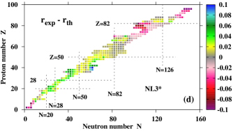
Figure 10: (Color online) The difference between measured and calculated charge radii $r_{ch}$ for indicated functionals. The experimental data are taken from Ref.  Angeli and Marinova (2013).

Table 10: The rms deviations $\Delta{E_{rms}}$, $\Delta{(S_{2n})_{rms}}$ ($\Delta{(S_{2p})_{rms}}$) and $\Delta{(r_{ch})_{rms}}$ between calculated and experimental binding energies $E$, two-neutron (-proton) separation energies $S_{2n}$ $(S_{2p})$ and charge radii $r_{ch}$ for indicated CEDFs. For first three observables, they are given with respect of ”measured” (640 nuclei) and ”measured+estimated” (830 nuclei) sets of experimental masses. For the calculations of the $\Delta{(r_{ch})_{rms}}$ values, all experimental data are used in column 6, while the data on radii of He ($Z=2$) and Cm ($Z=96$) isotopes are excluded in column 7. See text for the discussion of these cases.

CEDF	measured	measured+estimated			charge radii
	$\Delta{E_{rms}}$ [MeV]	$\Delta{E_{rms}}$ [MeV]	$\Delta{(S_{2n})_{rms}}$ [MeV]	$\Delta{(S_{2p})_{rms}}$ [MeV]	$\Delta{(r_{ch})_{rms}}$ [fm]	$\Delta{(r_{ch})_{rms}}$ [fm]
1	2	3	4	5	6	7
NL5(C)	3.41	3.71	1.37	1.54	0.040	0.0284
NL5(D)	2.83	2.90	1.22	1.29	0.041	0.0277
NL5(E)	2.73	2.81	1.23	1.29	0.042	0.0288
NL3*	2.96	3.00	1.23	1.29	0.041	0.0283

Table 11: The values of the parameters of different sets for the finite range Gogny forces (see equations in the appendix of Ref. Berger et al. (1991) or Eq. (3) in Ref. Goriely et al. (2009) for the definition of the Gogny force). The $\mu_{i}$ $(i=1,2)$ parameters describe the range of the interaction. The strength of the Wigner, Bartlett, Heisenberg and Majorana terms is given by $W_{i}$, $B_{i}$, $H_{i}$ and $M_{i}$, respectively. The parameters $t_{0}$, $x_{0}$ and $\alpha$ define the density dependence of the interaction, while $W_{LS}$ zero-range two-body spin-orbit interaction.

Parameters	D1SBerger et al. (1991)		D1Gogny (1975)		D1MGoriely et al. (2009)
$\mu_{i}$ (fm)	0.7	1.2	0.7	1.2	0.5	1.0
$W_{i}$ [MeV]	-1720.30	103.64	-402.4	-21.30	-12797.57	490.95
$B_{i}$ [MeV]	1300.00	-163.48	-100.0	-11.77	14048.85	-752.27
$H_{i}$ [MeV]	-1813.53	162.81	-496.2	37.27	-15144.43	675.12
$M_{i}$ [MeV]	1397.60	-223.93.	-23.56	-68.81	11963.89	-693.57
$t_{0}$ [MeV]	1390.6		1350.0		1562.22
$x_{0}$	1		1		1
$\alpha$	1/3		1/3		1/3
$W_{LS}$ [MeV]	-130.0		115.0		115.56

Table 12: The values of the parameters for different Skyrme forces. When needed the parameters are reduced to the form of the Skyrme force employed for the BSk class of the functionals (see Eq. (1) in Ref. Goriely et al. (2013)). The parameters $t_{0}$ and $x_{0}$ define the central term. $t_{1}$, $x_{1}$, $t_{2}$, $x_{2}$ are the parameters of the non-local terms. Density dependence is defined by $t_{3}$, $x_{3}$ and $\gamma$ parameters. The $W_{0}$ and $W_{1}$ parameters define the spin-orbit interaction. The BSk28 and BSk29 functionals have many additional parameters as compared with other functionals; some of them ($t_{4}$, $x_{4}$, $t_{5}$, $x_{5}$) are shown here but others (see 9 bottom lines of Table 1 in Ref.  Goriely (2015)) are omitted for simplicity.

Parameters	UNEDF0 Kortelainen et al. (2010)	UNEDF1 Kortelainen et al. (2012)	SLy4 Chabanat et al. (1998)	SKM* Bartel et al. (1982)	BSk28 Goriely (2015)	BSk29 Goriely (2015)
$t_{0}[MeVfm^{3}]$	-1883.68781034	-2078.32802326	-2488.91	-2645.00	-3988.86	-3970.40
$t_{1}[MeVfm^{5}]$	277.50021224	239.40081204	486.82	410.00	395.769	394.880
$t_{2}[MeVfm^{5}]$	608.43090559	1575.11954190	-546.39	-135.00
$t_{3}[MeVfm^{3+3\alpha}]$	13901.94834463	14263.64624708	13777.0	15595.0	22774.4	22649.3
$t_{4}[MeVfm^{5+3\beta}]$					-100.000	-100.000
$t_{5}[MeVfm^{5+3\gamma}]$					-150.000	-150.000
$x_{0}$	0.00974375	0.05375692	0.834	0.09	0.928026	0.964850
$x_{1}$	-1.77784395	-5.07723238	-0.344	0.00	0.0274980	-0.0047741
$x_{2}$	-1.67699035	-1.36650561	-1.000	0.00
$t_{2}x_{2}[MeVfm^{5}]$					-1388.61	-1388.95
$x_{3}$	-0.38079041	-0.16249117	1.354	0.00	1.09482	1.14453
$x_{4}$					2.0000	2.00000
$x_{5}$					-11.0000	-11.0000
$W_{0}[MeVfm^{5}]$	33.9006	109.6845943	123.0	130.0	80.489	64.600
$W_{1}[MeVfm^{5}]$					180.411	0
$\alpha$	0.32195599	0.27001801	1/6	1/6	1/12	1/12
$\beta$					1/2	1/2
$\gamma$					1/12	1/12
$\nu$					1	0
$y_{\omega}$					0	2

Another example is time-odd mean fields. They have an impact on a considerable number of physical observables in the systems with broken time-reversal symmetries Vretenar et al. (2005); Afanasjev and Abusara (2010a). However, their impact depends on the $g_{\omega}$ and $m_{\omega}$ parameters Afanasjev and Abusara (2010a, b), which according to our results vary very little (see Fig. 2a, b, c, 5b and 6b). Note that $m_{\omega}$ is fixed in many functionals. These facts suggest that statistical errors in time-odd mean fields and the components of physical observables related to time-odd mean fields (such as the contribution to the moment of inertia due to time-odd mean fields Afanasjev and Abusara (2010b) or additional binding due to nuclear magnetism Afanasjev and Abusara (2010a)) should be reasonably small.

VIII ACKNOWLEDGMENTS

This material is based upon work supported by the U.S. Department of Energy, Office of Science, Office of Nuclear Physics under Award No. DE-SC0013037.

Appendix A Global performance of the NL5(*) covariant energy density functionals

The global performance of the NL5(C), NL5(D) and NL5(E) functionals in the description of ground state properties of even-even nuclei is presented in Figs. 9 and 10 and summarized in Table 10. Experimental data on binding energies of 835 even-even nuclei is taken from Ref.  Wang et al. (2012); note that there are 640 measured and 195 estimated masses of even-even nuclei in the AME2012 mass evaluation. Experimental data on charge radii of 351 even-even nuclei is taken from Ref. Angeli and Marinova (2013). The global performance of the NL5(*) functionals is also compared with the one of the NL3* functional studied in details in Refs. Agbemava et al. (2014, 2015); Afanasjev and Agbemava (2016). Note that the NL3* is the state-of-the-art functional for the non-linear coupling meson exchange models (see Ref. Agbemava et al. (2014)) with well documented record of successful applications to the ground state properties of even-even nuclei Lalazissis et al. (2009); Agbemava et al. (2014); Afanasjev and Agbemava (2016), octupole deformation in the ground states of even-even nuclei Agbemava et al. (2016), giant resonances Lalazissis et al. (2009), the energies and spectroscopic factors of dominant components of single-particle states in odd-mass nuclei Litvinova and Afanasjev (2011); Afanasjev and Litvinova (2015), rotating nuclei Lalazissis et al. (2009); Afanasjev and Abdurazakov (2013), fission barriers Abusara et al. (2010, 2012), superheavy nuclei Agbemava et al. (2015) etc.

The rms deviations $\Delta{E_{rms}}\sim 3.7$ MeV between calculated and experimental binding energies $E$ for the NL5(C) CEDF are very similar to those obtained with original NL3 functional (see Ref. Lalazissis et al. (1999)). The NL3* functional Lalazissis et al. (2009); Agbemava et al. (2014) with $\Delta{E_{rms}}=3.0$ MeV represents an improved version of this functional. The NL5(D) and especially NL5(E) functionals provide further improvement of global description of masses as compared with the NL3* one (see Table 10). They produce comparable with NL3* description of two-neutron ($S_{2n}$) and two-proton ($S_{2n}$) separation energies (see Table 10). With minor differences the distribution of the $E_{th}-E_{exp}$ quantities in the $(Z,N)$ plane is similar for the NL5(D), NL5(E) and NL3* functionals (Fig. 9). On the contrary, there are substantial differences between the NL5(C) and NL3* functionals in that respect.

All functionals give comparable rms deviations for charge radii $\Delta(r_{ch})_{rms}$ (see Table 10). Note that the last column in Table 10 excludes experimental data on He ($Z=2$) (3 data points) and Cm ($Z=96$) (4 data points) nuclei (see detailed motivation in Sect. X of Ref. Agbemava et al. (2014)). It is clear that DFTs cannot describe very light nuclei such as He. In addition, experimental charge radii of the Cm ($Z=96$) nuclei are lower than those of Pu ($Z=94$) and U ($Z=92$) Angeli and Marinova (2013). Such feature goes against a general trend of the increase of charge radii with the increase of proton number for comparable deformations and could be described neither in CDFT (see Ref. Agbemava et al. (2014)) nor in non-relativistic DFT calculations with Gogny D1S functional (see Supplemental Material to Ref. Delaroche et al. ).

Appendix B The examples of the spread of the parameters in non-relativistic functionals

Tables 11 and 12 illustrate the spread of model parameters in the Gogny and Skyrme energy density functionals. These are state-of-the-art finite range Gogny functionals D1S Berger et al. (1991) and D1M Goriely et al. (2009) and state-of-the-art zero-range Skyrme functionals UNEDF0 Kortelainen et al. (2010), UNEDF1Kortelainen et al. (2012), BSk28 Goriely (2015) and BSk29 Goriely (2015). They are compared with older Skyrme functionals SLy4 Chabanat et al. (1998) and SkM* Bartel et al. (1982) and first Gogny functional D1 Gogny (1975). Apart of D1, all other functionals are still in extensive use.

D1 Gogny (1975) is the first Gogny functional. However, it was found in Ref. Berger et al. (1984) that it does not reproduce fission barriers in actinides. Thus, the D1S functional was fitted in Ref. Berger et al. (1984): fitting protocol of this functional includes experimental data on fission barriers in addition to the data used in the fitting protocol of the D1 functional. One can see in Table 11 that for the same radial ranges $\mu_{i}$ of the D1 and D1S forces, the absolute values of the strength parameters $W_{i}$, $B_{i}$, $H_{i}$ and $M_{i}$ of the central force of D1S differ by almost an order of magnitude from those of D1. In addition, the strength $W_{LS}$ of the spin-orbit interaction has different signs in these two functionals. The D1S functional has been successfully applied to the description of many nuclear phenomena Peru and Martini (2014) and it is still widely used by many practitioners of the Gogny DFT. The D1M functional has been fitted globally to nuclear masses in Ref. Goriely et al. (2009). Shorter ranges of interaction are used in it (see Table 11); as a result, the strenghts of the central force terms change (as compared with D1S) by approximately one order of magnitude for $i=1$ and by a factor of approximately 4 for $i=2$. As compared with D1S, the $t_{0}$ strength is modified by more that 10% but the strength of spin-orbit interaction remains unchanged.

Contrary to the Gogny functionals there is significant number of Skyrme energy density functionals (SEDF); the compilation of Ref. Dutra et al. (2012) reveals 240 SEDFs developed by 2012. However, one should recognize that only small subset of these functionals is used in the calculations of finite nuclei in a repetitive manner. Table 12 lists some of them. As compared with Gogny functionals shown in Table 12, the variations in the parameters of SEDF (see Table 12) are less drastic. However, even the parameters of recent classes of the SEDF, namely UNEDF* Kortelainen et al. (2010, 2012) and BSk* Goriely (2015), differ substantially. This reflects the differences in the form of SEDFs and the details of the fitting protocols; see also Sect. 5.C. of Ref. Bender et al. (2003) for short review of fitting protocols employed in nuclear DFTs.

These results clearly show the difference between relativistic and non-relativistic DFTs. In CDFT, the parameters of the $\sigma$- and $\omega$-mesons are well localized for all functionals (see Fig. 2) independent of the form of the density dependence, the properties of the $\rho$-meson or the details of the fitting protocol. Basically starting from first successful CEDF NL1 Reinhard et al. (1986), fitted 33 years ago, the parameters of the $\sigma$- and $\omega$-mesons of all successful functionals developed over the years and quoted in the present manuscript are very close to each other (see Fig. 2). This is due to the fact that nucleonic potential in CDFT is build as a sum of large attractive scalar potential (related to $\sigma$-meson) and large repulsive vector potential (related to $\omega$-meson) which limits possible range of the variations of the parameters. On the contrary, as illustrated in Tables 11 and 12 the level of the localization of the parameters is lower (and the spread of the parameters is higher) in non-relativistic functionals.

References

- Reinhard and Nazarewicz (2010) P. G. Reinhard and W. Nazarewicz, Phys. Rev. C 81, 051303(R) (2010).
- Dobaczewski et al. (2014) J. Dobaczewski, W. Nazarewicz, and P.-G. Reinhard, J. Phys. G 41, 074001 (2014).
- Agbemava et al. (2014) S. E. Agbemava, A. V. Afanasjev, D. Ray, and P. Ring, Phys. Rev. C 89, 054320 (2014).
- Erler et al. (2012) J. Erler, N. Birge, M. Kortelainen, W. Nazarewicz, E. Olsen, A. M. Perhac, and M. Stoitsov, Nature 486, 509 (2012).
- Afanasjev et al. (2013) A. V. Afanasjev, S. E. Agbemava, D. Ray, and P. Ring, Phys. Lett. B 726, 680 (2013).
- Gao et al. (2013) Y. Gao, J. Dobaczewski, M. Kortelainen, J. Toivanen, and D. Tarpanov, Phys. Rev. C 87, 034324 (2013).
- McDonnell et al. (2015) J. D. McDonnell, N. Schunck, D. Higdon, J. Sarich, S. M. Wild, and W. Nazarewicz, Phys. Rev. Lett. 114, 122501 (2015).
- Martin et al. (2016) D. Martin, A. Arcones, W. Nazarewicz, and E. Olsen, Phys. Rev. Lett. 116, 121101 (2016).
- Mumpower et al. (2016) M. R. Mumpower, R. Surman, G. C. McLaughlin, and A. Aprahamian, Prog. Part. Nucl. Phys. 86, 86 (2016).
- Lovell et al. (2017) A. E. Lovell, F. M. Nunes, J. Sarich, and S. M. Wild, Phys. Rev. C 95, 024611 (2017).
- Brandt (2014) S. Brandt, Data analysis. Statistical and Computational Methods for Scientists and Engineers. (Springer International Publishing, Switzerland, 2014).
- Bender et al. (2003) M. Bender, P.-H. Heenen, and P.-G. Reinhard, Rev. Mod. Phys. 75, 121 (2003).
- Boguta and Bodmer (1977) J. Boguta and R. Bodmer, Nucl. Phys. A292, 413 (1977).
- Peru and Martini (2014) S. Peru and M. Martini, Eur. Phys. J 50, 88 (2014).
- Vretenar et al. (2005) D. Vretenar, A. V. Afanasjev, G. A. Lalazissis, and P. Ring, Phys. Rep. 409, 101 (2005).
- Lalazissis et al. (2005) G. A. Lalazissis, T. Nikšić, D. Vretenar, and P. Ring, Phys. Rev. C 71, 024312 (2005).
- Lalazissis et al. (2009) G. A. Lalazissis, S. Karatzikos, R. Fossion, D. P. Arteaga, A. V. Afanasjev, and P. Ring, Phys. Lett. B671, 36 (2009).
- Nikšić et al. (2008) T. Nikšić, D. Vretenar, and P. Ring, Phys. Rev. C 78, 034318 (2008).
- Typel and Wolter (1999) S. Typel and H. H. Wolter, Nucl. Phys. A656, 331 (1999).
- LNP (2004) Extended Density Functionals in Nuclear Structure Physics, Lecture Notes in Physics, edited by G. A. Lalazissis, P. Ring, and D. Vretenar (Springer-Verlag, Heidelberg, 2004) Vol. 641 (2004).
- Litvinova and Afanasjev (2011) E. V. Litvinova and A. V. Afanasjev, Phys. Rev. C 84, 014305 (2011).
- Cohen et al. (1992) T. D. Cohen, R. J. Furnstahl, and K. Griegel, Phys. Rev. C 45, 1881 (1992).
- Koepf and Ring (1989) W. Koepf and P. Ring, Nucl. Phys. A 493, 61 (1989).
- Afanasjev and Abusara (2010a) A. V. Afanasjev and H. Abusara, Phys. Rev. C 81, 014309 (2010a).
- Meng et al. (2006) J. Meng, H. Toki, S. G. Zhou, S. Q. Zhang, W. H. Long, and L. S. Geng, Prog. Part. Nucl. Phys. 57, 470 (2006).
- Nikšić et al. (2011) T. Nikšić, D. Vretenar, and P. Ring, Prog. Part. Nucl. Phys. 66, 519 (2011).
- RDF (2016) “Relativistic Density Functional for Nuclear Structure”, (World Scientific Publishing Co), Edited by Jie Meng, Int. Rev. Nucl. Phys. 10 (2016).
- Afanasjev et al. (2015) A. V. Afanasjev, S. E. Agbemava, D. Ray, and P. Ring, Phys. Rev. C 91, 014324 (2015).
- Agbemava et al. (2015) S. E. Agbemava, A. V. Afanasjev, T. Nakatsukasa, and P. Ring, Phys. Rev. C 92, 054310 (2015).
- Agbemava et al. (2016) S. E. Agbemava, A. V. Afanasjev, and P. Ring, Phys. Rev. C 93, 044304 (2016).
- Afanasjev and Agbemava (2016) A. V. Afanasjev and S. E. Agbemava, Phys. Rev. C 93, 054310 (2016).
- Agbemava and Afanasjev (2017) S. E. Agbemava and A. V. Afanasjev, Phys. Rev. C 96, 024301 (2017).
- Agbemava et al. (2017) S. E. Agbemava, A. V. Afanasjev, D. Ray, and P. Ring, PRC 95 (2017).
- Afanasjev and Shawaqfeh (2011) A. V. Afanasjev and S. Shawaqfeh, Phys. Lett. B 706, 177 (2011).
- Dobaczewski et al. (2015) J. Dobaczewski, A. V. Afanasjev, M. Bender, L. M. Robledo, and Y. Shi, Nucl. Phys. A 944, 388 (2015).
- Afanasjev and Abdurazakov (2013) A. V. Afanasjev and O. Abdurazakov, Phys. Rev. C 88, 014320 (2013).
- Debes and Dudek (2017) I. Debes and J. Dudek, Acta Phys. Polonica B10, 51 (2017).
- Niksic et al. (2015) T. Niksic, N. Paar, P.-G. Reinhard, and D. Vretenar, J. Phys. G 42, 034008 (2015).
- Haverinen and Kortelainen (2017) T. Haverinen and M. Kortelainen, J. Phys. G 44, 044008 (2017).
- Bürvenich et al. (2004) T. Bürvenich, D. Madland, and P.-G. Reinhard, Nucl. Phys. A 744, 92 (2004).
- Birge (1932) R. T. Birge, Phys. Rev. 40, 207 (1932).
- Serot and Walecka (1986) B. D. Serot and J. D. Walecka, Adv. Nucl. Phys. 16, 1 (1986).
- Gambhir et al. (1990) Y. K. Gambhir, P. Ring, and A. Thimet, Ann. Phys. (N.Y.) 198, 132 (1990).
- Kohn and Sham (1965) W. Kohn and L. J. Sham, Phys. Rev. 137, A1697 (1965).
- Tian et al. (2009) Y. Tian, Z. Y. Ma, and P. Ring, Phys. Lett. B 676, 44 (2009).
- Reinhard et al. (1986) P.-G. Reinhard, M. Rufa, J. Maruhn, W. Greiner, and J. Friedrich, Z. Phys. A 323, 13 (1986).
- Rufa et al. (1988) M. Rufa, P.-G. Reinhard, J. A. Maruhn, W. Greiner, and M. R. Strayer, Phys. Rev. C 38, 390 (1988).
- Sharma et al. (1993) M. Sharma, M. Nagarajan, and P. Ring, Phys. Lett. B 312, 377 (1993).
- Lalazissis et al. (1997) G. A. Lalazissis, J. König, and P. Ring, Phys. Rev. C 55, 540 (1997).
- Dutra et al. (2014) M. Dutra, O. Lourenco, S. S. Avancini, B. V. Carlson, A. Delfino, D. P. Menezes, C. Providencia, S. Typel, and J. R. Stone, Phys. Rev. C 90, 055203 (2014).
- Abrahamyan et al. (2012) S. Abrahamyan et al., Phys. Rev. Lett. 108, 112502 (2012).
- (52) The PREX-II proposal, unpublished, available at hallaweb.jlab.org/parity/prex .
- Krasznahorkay et al. (1999) A. Krasznahorkay, M. Fujiwara, P. van Aarle, H. Akimune, I. Daito, H. Fujimura, Y. Fujita, M. N. Harakeh, T. Inomata, J. Jänecke, S. Nakayama, A. Tamii, M. Tanaka, H. Toyokawa, W. Uijen, and M. Yosoi, Phys. Rev. Lett. 82, 3216 (1999).
- Yako et al. (2006) K. Yako, H. Sagawa, and H. Sakai, Phys. Rev. C 74, 051303 (2006).
- Tarbert et al. (2014) C. M. Tarbert, D. P. Watts, D. I. Glazier, P. Aguar, J. Ahrens, J. R. M. Annand, H. J. Arends, R. Beck, V. Bekrenev, B. Boillat, A. Braghieri, D. Branford, W. J. Briscoe, J. Brudvik, S. Cherepnya, R. Codling, E. J. Downie, K. Foehl, P. Grabmayr, R. Gregor, E. Heid, D. Hornidge, O. Jahn, V. L. Kashevarov, A. Knezevic, R. Kondratiev, M. Korolija, M. Kotulla, D. Krambrich, B. Krusche, M. Lang, V. Lisin, K. Livingston, S. Lugert, I. J. D. MacGregor, D. M. Manley, M. Martinez, J. C. McGeorge, D. Mekterovic, V. Metag, B. M. K. Nefkens, A. Nikolaev, R. Novotny, R. O. Owens, P. Pedroni, A. Polonski, S. N. Prakhov, J. W. Price, G. Rosner, M. Rost, T. Rostomyan, S. Schadmand, S. Schumann, D. Sober, A. Starostin, I. Supek, A. Thomas, M. Unverzagt, T. Walcher, L. Zana, and F. Zehr (Crystal Ball at MAMI and A2 Collaboration), Phys. Rev. Lett. 112, 242502 (2014).
- Reinhard (1989) P.-G. Reinhard, Rep. Prog. Phys. 52, 439 (1989).
- Ring (1996) P. Ring, Prog. Part. Nucl. Phys. 37 (1996).
- Bender et al. (1999) M. Bender, K. Rutz, P.-G. Reinhard, J. A. Maruhn, and W. Greiner, Phys. Rev. C 60, 034304 (1999).
- Rashdan (2001) M. Rashdan, Phys. Rev. C 63, 044303 (2001).
- Long et al. (2004) W. Long, J. Meng, N. V. Giai, and S.-G. Zhou, Phys. Rev. C 69, 034319 (2004).
- Ren and Toki (2001) Z. Ren and H. Toki, Nucl. Phys. A 689, 691 (2001).
- Sugahara and Toki (1994) Y. Sugahara and H. Toki, Nucl. Phys. A 579, 557 (1994).
- Nikšić et al. (2002) T. Nikšić, D. Vretenar, P. Finelli, and P. Ring, Phys. Rev. C 66, 024306 (2002).
- Roca-Maza et al. (2011) X. Roca-Maza, X. Viñas, M. Centelles, P. Ring, and P. Schuck, Phys. Rev. C 84, 054309 (2011).
- Nikšić et al. (2017) T. Nikšić, M. Imbrišak, and D. Vretenar, Phys. Rev. C 95, 054304 (2017).
- Kortelainen et al. (2013) M. Kortelainen, J. Erler, W. Nazarewicz, N. Birge, Y. Gao, and E. Olsen, Phys. Rev. C 88, 031305(R) (2013).
- Afanasjev and Litvinova (2015) A. V. Afanasjev and E. Litvinova, Phys. Rev. C 92, 044317 (2015).
- Bender et al. (2001) M. Bender, W. Nazarewicz, and P.-G. Reinhard, Phys. Lett. B 515, 42 (2001).
- Afanasjev et al. (2003) A. V. Afanasjev, T. L. Khoo, S. Frauendorf, G. A. Lalazissis, and I. Ahmad, Phys. Rev. C 67, 024309 (2003).
- Afanasjev (2015) A. V. Afanasjev, J. Phys. G 42, 034002 (2015).
- Afanasjev and Abusara (2010b) A. V. Afanasjev and H. Abusara, Phys. Rev. C 82, 034329 (2010b).
- Wang et al. (2012) M. Wang, G. Audi, A. H. Wapstra, F. G. Kondev, M. MacCormick, X. Xu, and B. Pfeiffer, Chinese Physics C36, 1603 (2012).
- Angeli and Marinova (2013) I. Angeli and K. P. Marinova, At. Data Nucl. Data Tables 99, 69 (2013).
- Abusara et al. (2010) H. Abusara, A. V. Afanasjev, and P. Ring, Phys. Rev. C 82, 044303 (2010).
- Abusara et al. (2012) H. Abusara, A. V. Afanasjev, and P. Ring, Phys. Rev. C 85, 024314 (2012).
- Lalazissis et al. (1999) G. A. Lalazissis, S. Raman, and P. Ring, At. Data Nucl. Data Table 71, 1 (1999).
- (77) J.-P. Delaroche, M. Girod, J. Libert, H. Goutte, S. Hilaire, S. Peru, N. Pillet, and G. F. Bertsch, .
- Berger et al. (1991) J. F. Berger, M. Girod, and D. Gogny, Comp. Phys. Comm. 63, 365 (1991).
- Goriely et al. (2009) S. Goriely, S. Hilaire, M. Girod, and S. Péru, Phys. Rev. Lett. 102, 242501 (2009).
- Gogny (1975) D. Gogny, in: G. Ripka, M. Porneuf (Eds.), Nuclear Self-Consistent Fields, Proc. Internat. Conf. held at the Center for Theoretical Physics, Trieste, Italy, 1975, North-Holland, Amsterdam , 333 (1975).
- Kortelainen et al. (2010) M. Kortelainen, T. Lesinski, J. Moré, W. Nazarewicz, J. Sarich, N. Schunck, M. V. Stoitsov, and S. Wild, Phys. Rev. C 82, 024313 (2010).
- Kortelainen et al. (2012) M. Kortelainen, J. McDonnell, W. Nazarewicz, P.-G. Reinhard, J. Sarich, N. Schunck, M. V. Stoitsov, and S. M. Wild, Phys. Rev. C 85, 024304 (2012).
- Goriely (2015) S. Goriely, Nuclear Physics A 933, 68 (2015).
- Chabanat et al. (1998) E. Chabanat, P. Bonche, P. Haensel, J. Meyer, and R. Schaeffer, Nucl. Phys. A635, 231 (1998).
- Bartel et al. (1982) J. Bartel, P. Quentin, M. Brack, C. Guet, and H.-B. Hakansson, Nucl. Phys. A386, 79 (1982).
- Berger et al. (1984) J. F. Berger, M. Girod, and D. Gogny, Nucl. Phys. A428, 23c (1984).
- Dutra et al. (2012) M. Dutra, O. Lourenco, J. S. S. Martins, A. Delfino, J. R. Stone, and P. D. Stevenson, Phys. Rev. C 85, 035201 (2012).
- Goriely et al. (2013) S. Goriely, N. Chamel, and J. M. Pearson, Phys. Rev. C 88, 061302 (2013).