Polarization in a three-dimensional Fermi gas with Rabi coupling

Abstract

We investigate the polarization of a two-component three-dimensional fermionic gas made of repulsive alkali-metal atoms. The two pseudo-spin components correspond to two hyperfine states which are Rabi coupled. The presence of Rabi coupling implies that only the total number of atoms is conserved and a quantum phase transition between states dominated by spin-polarization along different axses is possible. By using a variational Hartree-Fock scheme we calculate analytically the ground-state energy of the system and determine analytically and numerically the conditions under which there is this quantum phase transition. This scheme includes the well-known criterion for the Stoner instability. The obtained phase diagram clearly shows that the polarized phase crucially depends on the interplay among the Rabi coupling energy, the interaction energy per particle, and the kinetic energy per particle.

1 Introduction

Few years ago, seminal experiments realized artificial spin-orbit and Rabi couplings in bosonic [1, 2] and fermionic [3, 4] atomic gases. In these experiments, laser beams were used to couple two internal hyperfine states of the atom by a stimulated two-photon Raman transition [1, 2, 3, 4]. Driven by these experiments, many papers have analyzed spin-orbit effects in Bose-Einstein condensates [5, 6, 7, 8, 9, 10, 11, 12, 13] and also in the BCS-BEC crossover of superfluid fermions [14, 15, 16, 17, 18, 19, 20, 21, 22, 23, 24].

Very recently, ferromagnetic instability has been reported in a two-component three-dimensional (3D) Fermi gas made of ultracold ⁶Li atoms [25]. The repulsive interaction between fermionic atoms induces the well-known Stoner instability [26] above a critical strength. In the absence of the Rabi coupling, the system remains balanced and this instability produces balanced ferromagnetism with phase separation rather than spin flip [27, 28, 29, 30, 31, 32]. In previous papers [33, 34] we have investigated the role of the Rabi coupling in a 2D Fermi gas to the formation of spin-flip, i.e. polarization [28]. In this 2D theoretical study the density of states is quite simple and the obtained phase diagram is fully analytical [34].

In this paper we study the emergence of polarization along the $z$ axis in a Rabi-coupled 3D Fermi gas of repulsive alkali-metal atoms. Unlike the 2D case, the 3D density of states is quite complex and requires an analytical study of the equation determining the ground state supported by numerical calculations. The fermionic atoms are characterized by two hyperfine internal states, which can be modelled as two spin components. We neglect the role of molecules which could be relevant in the presence of strong spin-component interaction. We analyze the ground-state properties of the quantum gas by using the variational Hartree-Fock method, where the population imbalance is a variational parameter. We determine analytically and, in some regions of the phase diagram, numerically the conditions under which there is a quantum transition from a phase dominated by spin-polarization along the $x$ axis to a spin-polarized one along the $z$ axis. We find that this quantum phase transition, which corresponds to a spontaneous symmetry breaking of the fermion polarization (population imbalance) between two degenerate values, appears at a critical interaction strength which depends on both the Rabi energy and the kinetic energy.

After rapidly reviewing, in section 2, the application of the mean-field Hartree-Fock method to the model Hamiltonian, in section 3, we present the central result of our study, the phase diagram of the 3D model. We show that two distinct regimes characterize the system: in the first regime the 3D density of states features a simple form which allows one to analytically derive the critical line separating the balanced from polarized phase. Conversely, in the second regime, the 3D density of states features a strong nonlinear dependence on the significant physical parameters and the derivation of the critical line requires a detailed analysis of the ground-state equation and the numerical solution thereof. This regime is discussed in section 4, while section 5 is devoted to the polarization properties of the system.

2 Field-theory Hamiltonian with Rabi coupling

A 3D fermionic gas including contact interaction and Rabi coupling is described by the model Hamiltonian

$${\hat{H}}=\int d^{3}{\bf r}\left[-\sum_{\sigma=\uparrow,\downarrow}\frac{\hbar^{2}}{2m}{\hat{\psi}}_{\sigma}^{+}\nabla^{2}{\hat{\psi}}_{\sigma}+g\ {\hat{n}}_{\uparrow}^{+}{\hat{n}}_{\downarrow}+\frac{\hbar\Omega}{2}\left({\hat{\psi}}_{\uparrow}^{+}{\hat{\psi}}_{\downarrow}+{\hat{\psi}}_{\downarrow}^{+}{\hat{\psi}}_{\uparrow}\right)\right]\;,$$ (1)

where ${\hat{n}}_{\sigma}={\hat{\psi}}_{\sigma}^{+}{\hat{\psi}}_{\sigma}$ is the local number density operator for atoms with spin $\sigma={\uparrow},{\downarrow}$, $g$ and $\Omega$ are the contact interaction and the Rabi coupling, respectively, and ${\hat{\psi}}_{\sigma}({\bf r})$ is the field operator which destroys a fermion of spin $\sigma$ at position ${\bf r}$. A good quantum number associated to $\hat{H}$ is the total fermion number

$${\hat{N}}={\hat{N}}_{\uparrow}+{\hat{N}}_{\downarrow}=\int\!d^{3}{\bf r}\left({\hat{\psi}}_{\uparrow}^{+}({\bf r}){\hat{\psi}}_{\uparrow}({\bf r})+{\hat{\psi}}_{\downarrow}^{+}({\bf r}){\hat{\psi}}_{\downarrow}({\bf r})\right)$$ (2)

since $[{\hat{N}},{\hat{H}}]=0$. Conversely, ${\hat{N}}_{\uparrow}$ and ${\hat{N}}_{\downarrow}$, the spin-up and spin-down relative numbers, do not represent conserved quantities because the Rabi-coupling term in $\hat{H}$ entails $[{\hat{N}}_{\uparrow},{\hat{H}}]\neq 0$ and $[{\hat{N}}_{\downarrow},{\hat{H}}]\neq 0$. Following the variational Hartree-Fock approach applied to the two-dimensional gas [34], Hamiltonian (1) can be reformulated in the mean-field form where the term ${\hat{n}}_{\uparrow}{\hat{n}}_{\downarrow}$ is expressed as

$${\hat{n}}_{\uparrow}^{+}{\hat{n}}_{\downarrow}\simeq n_{\downarrow}\ {\hat{n}}_{\uparrow}^{+}+n_{\uparrow}\ {\hat{n}}_{\downarrow}^{+}-n_{\uparrow}\,n_{\downarrow},$$ (3)

by using the well-known mean-field (MF) formula for operator products [35, 36, 37]. This shows how the two spin components are coupled through the variational parameters $n_{\sigma}=\langle{\hat{n}}_{\sigma}\rangle$ while the resulting MF Hamiltonian assumes a quadratic form in terms of fields ${\hat{\psi}}_{\sigma}^{+}$ and ${\hat{\psi}}_{\sigma}$

$${\hat{H}}=\int d^{3}{\bf r}\left\{\left({\hat{\psi}}_{\uparrow}^{+},{\hat{\psi}}_{\downarrow}^{+}\right)\ {\cal H}\ \left(\begin{array}[]{c}{\hat{\psi}}_{\uparrow}\\ {\hat{\psi}}_{\downarrow}\end{array}\right)\right\}-{gn^{2}\over 4}(1-\zeta^{2})L^{3}\;,$$ (4)

where $L^{3}$ is the volume of the 3D system and

$${\cal H}=-\frac{\hbar^{2}}{2m}\nabla^{2}+\frac{gn}{2}{\mathbb{I}}-\frac{gn}{2}\zeta\sigma_{z}+\frac{\hbar\Omega}{2}\sigma_{x}\;,$$ (5)

has been expressed by using Pauli matrices $\sigma_{z}$ and $\sigma_{x}$ with $\zeta=(n_{\uparrow}-n_{\downarrow})/n$. To reduce such Hamiltonian to the diagonal form one first express ${\hat{\psi}}_{\sigma}^{+}$ and ${\hat{\psi}}_{\sigma}$ through the standard representation involving momentum-mode operators ${\hat{b}}^{+}_{{\bf k}\sigma}$ and ${\hat{b}}_{{\bf k}\sigma}$ and then implement the unitary transformations

$${\hat{b}}_{{\bf k}\uparrow}=C\ {\hat{b}}_{{\bf k},+}+S\ {\hat{b}}_{{\bf k},-},\quad{\hat{b}}_{{\bf k}\downarrow}=C\ {\hat{b}}_{{\bf k},-}-S\ {\hat{b}}_{{\bf k},+},$$ (6)

where the new ladder operators ${\hat{b}}_{{\bf k},s}$ and ${\hat{b}}_{{\bf k},s}^{+}$ have been defined and $C=\cos\phi/2$ and $S=\sin\phi/2$. The diagonal form is achieved when the angle $\phi$ is given by

$${\rm tg}\phi={\hbar\Omega}/(\zeta{gn})\ .$$ (7)

As a consequence, Hamiltonian (1) can be written as

$${\hat{H}}=-{gn^{2}\over 4}(1-\zeta^{2})L^{3}+\sum_{\bf k}\sum_{s=-1,1}E_{{\bf k},s}\ {\hat{b}}_{{\bf k},s}^{+}\ {\hat{b}}_{{\bf k},s}\;,$$ (8)

in which the energy eigenvalues read

$$E_{{\bf k},s}=\frac{\hbar^{2}k^{2}}{2m}+\alpha_{s}$$ (9)

with

$$\alpha_{s}=\frac{g}{2}{n}+{s\over 2}\;R\;,\quad\quad\quad R=\sqrt{{g^{2}n^{2}}\zeta^{2}+{\hbar^{2}\Omega^{2}}}.$$ (10)

A couple of parameters emerge from this approach

$$n=n_{\uparrow}+n_{\downarrow},\qquad\zeta={n_{\uparrow}-n_{\downarrow}\over n},$$ (11)

which represent the average total number density and the population imbalance, respectively. According with the current Hartree-Fock MF scheme, $\zeta$ represents the variational parameter of the model whose value can be determined by minimizing the total energy. At fixed total density ${n}$, the natural range of the imbalance parameter turns out to be $\zeta\in[-1,1]$.

3 Ground-state energy and phase diagram

In order to obtain an explicit analytic formula for both the total energy and the total particle number it advantageous to recast these quantities into the form

$$E={gn^{2}\over 4}(\zeta^{2}-1)L^{3}+\sum_{s}\frac{L^{3}}{8\pi^{3}}\int\!d^{3}{k}\;E_{{\bf k},s}n_{s}(k)\;,$$ (12)

$$N=\sum_{s}\frac{L^{3}}{(2\pi)^{3}}\int\!d^{3}k\;n_{s}(k)\,,$$ (13)

respectively, in which the continuum limit has been performed on the summations involving the momentum vector ${\bf k}$. The use of the zero-temperature fermionic densities $n_{s}(k)=\langle{\hat{b}}_{{\bf k},s}^{+}\ {\hat{b}}_{{\bf k},s}\rangle$ $=\theta\bigl{(}\mu-E(k,s)\bigr{)}=\theta\bigl{(}\mu-(q+\alpha_{s})\bigr{)}$ with $\theta(x)$ the Heaviside step function and $q=\hbar^{2}k^{2}/(2m)$, provides, after straightforward calculations, the total-energy density

$${\cal E}=\frac{gn^{2}}{4}(\zeta^{2}-1) + \!\frac{2}{(2\pi)^{2}}\left(\frac{2m}{\hbar^{2}}\right)^{3/2}\times$$

$$\sum_{s=\pm}\Bigl{[}\frac{(\mu-\alpha_{s})^{5/2}}{5} + \!\frac{\alpha_{s}}{3}(\mu-\alpha_{s})^{3/2}\Bigr{]}\ \theta(\mu-\alpha_{s}),$$ (14)

where ${\cal E}=E/L^{3}=\langle{\hat{H}}\rangle/L^{3}$, and the total number density

$$n=\frac{1}{6\pi^{2}}\left(\frac{2m}{\hbar^{2}}\right)^{3/2}\Bigl{[}(\mu-\alpha_{+})^{3/2}\theta(\mu-\alpha_{+})+(\mu-\alpha_{-})^{3/2}\theta(\mu-\alpha_{-})\Bigr{]},$$ (15)

where $n=N/L^{3}=\langle{\hat{N}}\rangle/L^{3}$ and $\alpha_{-}$ and $\alpha_{+}$ are given by Eq. (10). In Eqs. (14) and (15) both ${\cal E}$ and $n$ depend on the chemical potential $\mu$ and the population imbalance $\zeta$. Also, we note that the definition of Fermi momentum $k_{F}=(3\pi^{2}n)^{1/3}$ for a two-component gas [38] is naturally involved in (15) which takes the form

$$\left(\frac{\hbar^{2}k^{2}_{F}}{2m}\right)^{3/2}=\frac{1}{2}\left[(\mu-\alpha_{+})^{3/2}\theta(\mu-\alpha_{+})+(\mu-\alpha_{-})^{3/2}\theta(\mu-\alpha_{-})\right].$$ (16)

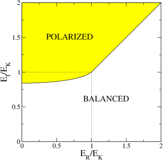
Figure 1: Phase diagram of in the plane $(E_{R}/E_{K},E_{I}/E_{K})$, where $E_{K}$ is the kinetic energy per particle, $E_{R}=\hbar\Omega$ is the Rabi energy, and $E_{I}=gn$ is the interaction energy per particle. Balanced means $\zeta=0$ and polarized means $\zeta\neq 0$.

In our approach (see also [34]), we first write ${\cal E}$ as function of $n$ and $\zeta$ and then we find the value of $\zeta$ which minimizes the energy density ${\cal E}$ at fixed total number density $n$. The procedure is repeated for different values of interaction strength $g$ and Rabi frequency $\Omega$. As suggested by equations (5), (14) and (16), we define the characteristic energy scales

$$E_{R}=\hbar\Omega\quad E_{I}=gn,\quad E_{K}=\frac{\hbar^{2}}{2m}(6\pi^{2}n)^{2/3}=2^{2/3}E_{F},$$ (17)

representing the Rabi energy, the interaction energy per particle, and the kinetic energy per particle, respectively. To favor the comparison with the Fermi-gas literature the latter has been also written in terms of the Fermi energy $E_{F}={\hbar^{2}k^{2}_{F}}/{(2m)}$. The extra factor $2^{2/3}$ bears memory of the fact that we deal with a two-component gas.

The main result of the paper is shown in Fig. 1, where we report the balanced-polarized phase diagram of the system in the plane $(E_{R}/E_{K},E_{I}/E_{K})$. The solid line is the critical curve of Stoner instability [26], where the uniform balanced configuration becomes unstable. The derivation of the phase diagram of Fig. 1 is discussed in detail for the two regimes $\alpha_{-}<\mu<\alpha_{+}$ and $\alpha_{\pm}<\mu$.

3.1 First regime

For $\alpha_{-}<\mu<\alpha_{+}$ formula (16) reduces to

$$\mu-\alpha_{-}=E_{K}$$ (18)

while the energy density becomes

$${\cal E}=\frac{n}{4}E_{I}(\zeta^{2}-1)+3n\left[\frac{E_{K}}{5}+\frac{E_{I}}{6}-\frac{1}{6}\sqrt{E_{I}^{2}\zeta^{2}+E_{R}^{2}}\right].$$ (19)

The characteristic energies (17) have been used. Then, one easily finds that the extremal values of $\cal E$ are determined by the condition

$$0=\frac{n}{2}E_{I}\zeta\left[1-\frac{E_{I}}{\sqrt{E_{I}^{2}\zeta^{2}+E_{R}^{2}}}\right].$$ (20)

The latter exhibits the two solutions $1)\,\,\zeta=0$ (for $E_{I}<E_{R}$) and $2)\,\,\zeta=\sqrt{1-{E_{R}^{2}}/{E_{I}^{2}}}$ (for $E_{I}>E_{R}$), with the energies

$${\cal E}_{1}=n\;\left(\frac{E_{I}}{4}+\frac{3E_{K}}{5}-\frac{E_{R}}{2}\right),\qquad{\cal E}_{2}=-\frac{E_{R}^{2}}{4g}+3n\frac{E_{K}}{5},$$ (21)

associated to $\mu_{1}=E_{K}+{(E_{I}-E_{R})}/{2}$, and $\mu_{2}=E_{K}$, respectively. One easily checks that ${\cal E}_{2}={\cal E}_{1}$ and $\mu_{1}=\mu_{2}$ at the critical value $E_{I}=E_{R}$. The inclusion of the constraint $\alpha_{-}<\mu<\alpha_{+}$ (characterizing the current case) rewritten as $E_{K}=\mu-\alpha_{-}<\alpha_{+}-\alpha_{-}$ (see (18)) entails, in turn,

$$E_{K}<\alpha_{+}-\alpha_{-}=\sqrt{E_{I}^{2}\zeta^{2}+E_{R}^{2}}.$$ (22)

This new constraint allows one to define the exact range of validity of the two solutions of equation (20), giving

$$1) \,\zeta=0\qquad{\rm for}\,\,\,E_{I}<E_{R},\,\,\,E_{K}<E_{R},$$ (23)

$$2) \,\zeta=\sqrt{1-\frac{E_{R}^{2}}{E_{I}^{2}}}\quad{\rm for}\,\,\,E_{R}<E_{I},\,\,\,E_{K}<E_{I}.$$ (24)

These well reproduce, in Fig. 1, the balanced-phase domain and polarized-phase domain, respectively, placed outside the squared box $E_{I},E_{R}<E_{K}$.

3.2 Second regime

This case is characterized by $\alpha_{\pm}<\mu$. Then, formula (15) becomes

$$E^{3/2}_{K}=(\mu-\alpha_{+})^{3/2}+(\mu-\alpha_{-})^{3/2},$$ (25)

where $E_{K}$ has been defined in equation (17). The constraint (25), in which $\alpha_{\pm}=(gn\pm R)/2$, causes the implicit dependence of $\mu$ from $R$, and thus from the mean-field parameter $\zeta$ contained in $R$. By introducing the new variables

$$\xi=(\mu-E_{I}/2)-R/2,\qquad\eta=(\mu-E_{I}/2)+R/2,$$ (26)

the constraint (25) becomes

$$E_{K}^{3/2}=\xi^{3/2}+\eta^{3/2},$$ (27)

where the fact that $\mu$ and $R$ (depending on $\zeta$) are independent variables implies that $\xi$ and $\eta$ are, in turn, independent variables. Equation (27) entails that the natural range of $\xi$ and $\eta$ is $\xi,\eta\in[0,E_{K}]$. In parallel, the use of variables $\xi$ and $\eta$ and of the explicit expressions of $\alpha_{\pm}$ in terms of $R$ and $ng=E_{I}$ in the energy density (14) (in which, now, $\theta(\mu-\alpha_{\pm})=1$) gives

$${\cal E}=\frac{n}{4}E_{I}(\zeta^{2}+1)+\frac{3n}{E_{K}^{3/2}}\left[\frac{\xi^{5/2}+\eta^{5/2}}{5}+\frac{R}{6}(\xi^{3/2}-\eta^{3/2})\right].$$ (28)

Then, by exploiting constraint (27), written in the form $\eta=(E_{K}^{3/2}-\xi^{3/2})^{2/3}$ in order to eliminate $\eta$ from $\cal E$, the energy density becomes

$${\cal E}=\frac{n}{4}E_{I}(\zeta^{2}+1)+\frac{3n}{E_{K}^{3/2}}\;G(\zeta),$$ (29)

where

$$G=G[R,\xi(R)]=\frac{1}{5}\xi^{5/2}+\frac{1}{5}\left(E_{K}^{3/2}-\xi^{3/2}\right)^{5/3}+\frac{R}{6}\left(2\xi^{3/2}-E_{K}^{3/2}\right).$$ (30)

Its derivative ${dG}/{d\zeta}$ can be easily calculated and, thanks to the identity $R=(E_{K}^{3/2}-\xi^{3/2})^{2/3}-\xi$, its final form is found to be

$$\frac{dG}{d\zeta}=\frac{2\xi^{3/2}-E_{K}^{3/2}}{6}\frac{dR}{d\zeta}=\left(2\xi^{3/2}-E_{K}^{3/2}\right)\frac{E_{I}^{2}\zeta}{6R}$$ (31)

where $R=\sqrt{E_{I}^{2}\zeta^{2}+E_{R}^{2}}$ has been used.

In conclusion, in the current regime where $\alpha_{\pm}<\mu$, one finds the energy-density derivative

$$\frac{d\cal E}{d\zeta}=\frac{nE_{I}}{2R}\zeta\left(R+\frac{2E_{I}}{E_{K}^{3/2}}\xi^{3/2}-E_{I}\right)=0$$ (32)

providing the explicit solution

$$\zeta=0,$$ (33)

and the implicitly-defined solution

$$R+\frac{2E_{I}}{E_{K}^{3/2}}\xi^{3/2}-E_{I}=0.$$ (34)

Equation (34) must be solved numerically. It is worth noting, however, that in the limit $\xi/E_{K}\ll 1$ (one should remind that this inequality corresponds to $\mu$ larger than, but very close to $\alpha_{+}$) the term $(\xi/E)^{3/2}$ can be neglected and $R-E_{I}\simeq 0$ entails $\zeta\simeq\pm\sqrt{1-E_{R}^{2}/E_{I}^{2}}$ with $E_{R}<E_{I}$. By keeping the approximation $(\xi/E)^{3/2}$ $\simeq 0$, the second derivative gives

$$\frac{d^{2}\cal E}{d\zeta^{2}}\simeq\frac{nE_{I}}{2R}\left(R-E_{I}\right)+\frac{nE_{I}^{2}}{2R^{3}}\zeta^{2}$$ (35)

showing that the first solution one finds, $\zeta=0$, is a minimum for $R=E_{R}>E_{I}$ and a maximum for $R=E_{R}<E_{I}$, whereas the second solution $\zeta\simeq$ $\pm\sqrt{1-E_{R}^{2}/E_{I}^{2}}$ is always a minimum provided that $E_{R}<E_{I}$. In the box $E_{I}/E_{K}\leq 1$, $E_{R}/E_{K}\leq 1$ (the region in Fig. 1 corresponding to the current regime $\alpha_{\pm}<\mu$) these results are in agreement with the presence of both the polarized phase ($E_{I}>E_{R}$ with $E_{I}/E_{K}>1$) and the balanced phases ($E_{I}<E_{R}$ with $E_{R}/E_{K}>1$) highlighted in regime $\alpha_{-}<\mu<\alpha_{+}$, and essentially represent the prolongation of such phases inside this box.

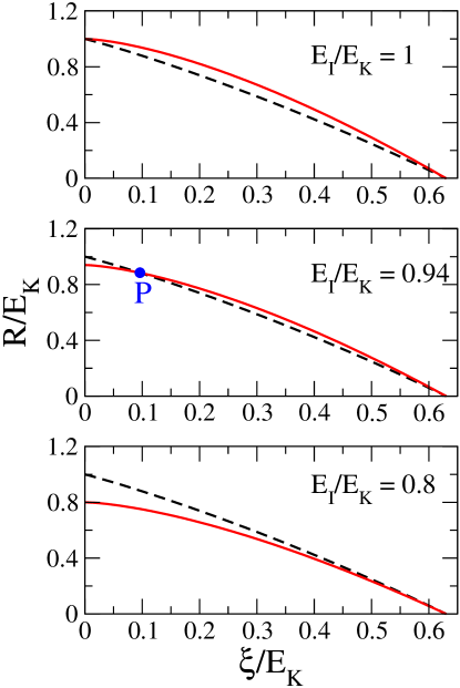
Figure 2: (Color Online) Curves describing $R/E_{K}$ vs $\xi/E_{K}$ according to Eqs. (36) and (37), which are, respectively, the solid line and the dashed line. The three panels correspond to different values of the adimensional interaction strength $E_{I}/E_{K}$. Only in the middle panel there is an intersection point $P$.

4 Phase boundary for $E_{R}<E_{K}$, $E_{I}<E_{K}$

The phase boundary inside the box $x=E_{R}/E_{K}<1$, $y=E_{I}/E_{K}<1$ of Fig. 1 is found by numerically calculating the values of $\zeta$ determined by means of equation (34) to minimize energy (29). Unlike the 2D case (see [34]), the separatrix between the polarized phase and the balanced phase is not a simple straight line intersecting the origin $x=y=0$ and bisecting the portion of plane $y\geq 0$, $x\geq 0$. This is due to the form of the equation (34) rewritten as

$$R=E_{I}\left(1-{2\xi^{3/2}}/{E_{K}^{3/2}}\right),$$ (36)

whose solution requires the use of the auxiliary equation

$$R=-\xi+\left(E_{K}^{3/2}-\xi^{3/2}\right)^{2/3}.$$ (37)

The latter, exhibiting a manifest nonlinear character, embodies the constraint (27), which due to $\eta-\xi=R$ (see equations (26)) implicitly defines $\xi$ as a function of $R$.

Despite the absence of an analytic explicit solution, some useful information can be extracted from such equations by representing them on the region of plane $(R,\xi)$ with $R,\xi\geq 0$ (see Fig. 2). With 1 and 2 referred to the functions (36) and (37), respectively, one observes that $R_{1}(\xi)=R_{2}(\xi)=0$ for $\xi=E_{K}/2^{2/3}$, while $R_{1}(0)=E_{I}$ and $R_{2}(0)=E_{K}$. In addition to $R_{1}(\xi)=R_{2}(\xi)=0$, equations (36) and (37) feature a second solution. This follows from the fact that $R_{1}(\xi)$ has zero derivative at $\xi=0$ whereas $R_{2}(\xi)$ is strongly decreasing for $\xi\simeq 0$. Then, for $E_{I}$ close enough to $E_{K}$, the two curves must intersect to each other in a single point. The derivatives $R_{1}^{\prime}(\xi)$ and $R_{2}^{\prime}(\xi)$ at $\xi_{0}=E_{K}/2^{2/3}$ provide the critical condition

$$R_{1}^{\prime}(\xi_{0})=-\frac{3E_{I}}{E_{K}2^{1/3}}\leq R_{2}^{\prime}(\xi)=-2,$$

stating that for $E_{I}\geq(2^{4/3}/3)E_{K}$ the two curves exhibit an intersection point P in the plane $(R,\xi)$, shown in the middle panel of Fig. 2. In parallel, the top panel in Fig. 2 shows how, for $E_{I}/E_{K}\equiv 1$, P reaches the point ($R=E_{K}$, $\xi=0$), while, for $E_{I}/E_{K}\equiv 2^{4/3}/3\simeq 0.8399$, the intersection point P tends to the point described by ($R=0$, $\xi_{0}=E_{K}/2^{2/3}$). Finally, the bottom panel in Fig. 2 highlights how, for $E_{I}/E_{K}<2^{4/3}/3$, no intersection survives.

By denoting with $A$ the portion of the yellow phase in the box $E_{I}/E_{K}\leq 1$, $E_{R}/E_{K}\leq 1$ of Fig. 1, one discovers that the interval $I=\{E_{I}/E_{K}\in[2^{4/3}/3,1]\}$ on the vertical axis actually represents the parameter range in which the system is in the polarized phase $|\zeta|\neq 0$ within the box. Particularly, any value $R_{*}=R(E_{I},E_{K})$ representing a solution of equations (33) and (34) for $E_{I}/E_{K}\in I$ allows one to determine $|\zeta|$ through the formula $R=(E_{I}^{2}|\zeta|^{2}+E_{R}^{2})^{1/2}$. The phase boundary confining $A$ from below is found as follows. Consider a specific horizontal (straight) line $y=E_{I}/E_{K}=const$ (with $E_{I}$, $E_{K}$ such that $E_{I}/E_{K}\in I$), crossing $A$ and intersecting the $A$ boundary. The resulting $|\zeta|$ is given by $|\zeta|=(R_{*}^{2}-E_{R}^{2})^{1/2}/E_{I}$. The two solutions $|\zeta|=R_{*}/E_{I}$, $E_{R}=0$ and $\zeta=0$, $E_{R}=R_{*}$ can be shown to be associated to the two intersection points of $y=E_{I}/E_{K}$ with $I$ (on the vertical axis) and the $A$ boundary, respectively. Intermediate values of $|\zeta|$ describe the points of the straight line inside $A$.

We conclude by noting how the Stoner condition $k_{F}=\pi/(2a)$, where $a$ is the scattering length of the interaction parameter $g=4\pi^{2}\hbar^{2}a/m$, for the transition to the polarized phase is recovered for $E_{R}=0$. In Fig. 1, the critical point corresponds to the lowest value $E_{I}/E_{K}=2^{4/3}/3$ of the interval $I$. Rewriting $E_{I}=gn$ as $E_{I}=gk_{F}^{3}/(3\pi^{2})$ the Stoner result is easily found.

We stress that the phase diagram of Fig. 1 is meaningful also in the presence of an external trapping potential $U({\bf r})$, where the total number density becomes space dependent, i.e. $n=n({\bf r})$. In this case, within the local density approximation, the fermionic cloud is fully balanced if $n({\bf r})^{1/3}<(2^{4/3}/3)\hbar^{2}(6\pi^{2})^{2/3}/(8\pi a)$ for any ${\bf r}$, while for $\Omega\neq 0$ the fermionic cloud can have an unbalanced region ${\cal D}$ under the condition $n({\bf r})^{1/3}>(2^{4/3}/3)(6\pi^{2})^{2/3}/(8\pi a)$ with ${\bf r}\in{\cal D}$. Due to the experimental flexibility of scattering and Rabi couplings, we believe our prediction can be tested by using available experimental setups with, for instance, ⁶Li atoms on a spherically-symmetric cloud of about 100 micron of radius.

5 Spin polarizations

The information emerging from our analysis and the phase diagram of Fig. 1 can be effectively represented by considering suitable indicators of the system polarization state. Let us consider the $z$ and $x$ components of the total spin operator

$${\hat{S}}_{z} = \frac{1}{2}\int d^{3}{\bf r}\ {\hat{\Psi}}^{+}\sigma_{z}{\hat{\Psi}}=\frac{1}{2}\int d^{3}{\bf r}\ \Bigl{(}{\hat{\psi}}^{+}_{\uparrow}{\hat{\psi}}_{\uparrow}-{\hat{\psi}}^{+}_{\downarrow}{\hat{\psi}}_{\downarrow}\Bigr{)}$$ (38)

$$= \frac{1}{2}\sum_{\bf k}\Bigl{(}{\hat{n}}_{{\bf k}\uparrow}-{\hat{n}}_{{\bf k}\downarrow}\Bigr{)},$$

$${\hat{S}}_{x} = \frac{1}{2}\int d^{3}{\bf r}\ {\hat{\Psi}}^{+}\sigma_{x}{\hat{\Psi}}=\frac{1}{2}\int d^{3}{\bf r}\ \Bigl{(}{\hat{\psi}}^{+}_{\uparrow}{\hat{\psi}}_{\downarrow}+{\hat{\psi}}^{+}_{\downarrow}{\hat{\psi}}_{\uparrow}\Bigr{)}$$ (39)

$$= \frac{1}{2}\sum_{\bf k}\Bigl{(}{\hat{b}}^{+}_{{\bf k}\uparrow}{\hat{b}}_{{\bf k}\downarrow}+{\hat{b}}^{+}_{{\bf k}\downarrow}{\hat{b}}_{{\bf k}\uparrow}\Bigr{)},$$

respectively, in which ${\hat{\Psi}}({\bf r})=({\hat{\psi}}_{\uparrow}({\bf r}),{\hat{\psi}}_{\downarrow}({\bf r}))$ is the two-component spinor. By using transformations (6) one finds

$${\hat{S}}_{z}=\sum_{\bf k}\Bigl{[}\frac{\cos\phi}{2}\Delta n_{\bf k}+\frac{\sin\phi}{2}({\hat{b}}^{+}_{{\bf k},+}{\hat{b}}_{{\bf k},-}+{\hat{b}}^{+}_{{\bf k},-}{\hat{b}}_{{\bf k},+})\Bigr{]},$$ (40)

$$S_{x}=\sum_{\bf k}\Bigl{[}\frac{\cos\phi}{2}({\hat{b}}^{+}_{{\bf k},+}{\hat{b}}_{{\bf k},-}+{\hat{b}}^{+}_{{\bf k},-}{\hat{b}}_{{\bf k},+})-\frac{\sin\phi}{2}\Delta n_{\bf k}\Bigr{]},$$ (41)

where the identities $\cos\phi\equiv\zeta E_{I}/R$, $\sin\phi\equiv E_{R}/R$ follow from equation (7), and

$$\Delta n_{\bf k}\equiv{\hat{n}}_{{\bf k},+}-{\hat{n}}_{{\bf k},-},\quad R=\sqrt{g^{2}n^{2}\zeta^{2}+\hbar^{2}\Omega^{2}}.$$ (42)

If state $|E_{0}\rangle=$ $\prod_{\bf k}|n_{{\bf k},+}\rangle|n_{{\bf k},-}\rangle$ is the ground state satisfying $H_{mf}|E_{0}\rangle=E_{0}|E_{0}\rangle$, then the expectation values

$$\langle E_{0}|{\hat{S}}_{z}|E_{0}\rangle=\frac{\zeta E_{I}}{2R}\sum_{\bf k}\langle E_{0}|\Delta n_{\bf k}|E_{0}\rangle,$$ (43)

$$\langle E_{0}|{\hat{S}}_{x}|E_{0}\rangle=\frac{E_{R}}{2R}\sum_{\bf k}\langle E_{0}|\Delta n_{\bf k}|E_{0}\rangle,$$ (44)

can be derived from (40) and (41). Eq. (43 ) can be rewritten in the more expressive way

$$\langle E_{0}|{\hat{S}}_{z}|E_{0}\rangle=\sum_{\bf k}\langle E_{0}|\frac{{\hat{n}}_{{\bf k}\uparrow}-{\hat{n}}_{{\bf k}\downarrow}}{2}|E_{0}\rangle=\frac{L^{3}}{2}(n_{\uparrow}-n_{\downarrow})$$ (45)

while the summation in the right-hand side of identities (43) and (44) can be shown to assume the form

$$\sum_{\bf k}\langle E_{0}|\Delta n_{\bf k}|E_{0}\rangle = \frac{nL^{3}}{E_{K}^{3/2}}\Bigl{[}(\mu-\alpha_{+})^{3/2}\theta(\mu-\alpha_{+})$$ (46)

$$- (\mu-\alpha_{-})^{3/2}\theta(\mu-\alpha_{-})\Bigr{]}.$$

Introducing equations (45) and (46) in (43) enables us to obtain the self-consistent equation characterizing our MF approach

$$\zeta\left[1+\frac{E_{I}}{RE_{K}^{3/2}}\sum_{p=\pm}\;p\left(\mu-\alpha_{p}\right)^{3/2}\theta\left(\mu-\alpha_{p}\right)\right]=0.$$ (47)

Thanks to the latter one has

$$\frac{RE_{K}^{3/2}}{ng}=(\mu-\alpha_{-})^{3/2}\theta(\mu-\alpha_{-})-(\mu-\alpha_{+})^{3/2}\theta(\mu-\alpha_{+}).$$

Therefore, equation (46) takes the form $\sum_{\bf k}\langle E_{0}|\Delta n_{{\bf k}}|E_{0}\rangle$ $=-{nL^{3}R}/{(gn)}$ and the average values $\langle{\hat{S}}_{z}\rangle$ and $\langle{\hat{S}}_{x}\rangle$ are simply given by

$$\langle{\hat{S}}_{z}\rangle={\zeta N}/{2},\quad\langle{\hat{S}}_{x}\rangle=-{NE_{R}}/{(2E_{I})}\;.$$ (48)

The first formula $\langle{\hat{S}}_{z}\rangle=N\zeta/2$ confirms the validity of the Hartree-Fock MF scheme showing how our variational Hartree-Fock method reproduces the correct description of the average polarization per particle of component ${\hat{S}}_{z}$ through the variational parameter $\zeta$. In the yellow area of Fig. (1), $\langle{\hat{S}}_{z}\rangle$ ranges from $N/2$ when $x=E_{R}/E_{K}=0$ to $\langle{\hat{S}}_{z}\rangle=0$ at any point of phase separatrix. On the other hand, the second formula in equation (48), describing the spin component ${\hat{S}}_{x}$ suggests that $\langle{\hat{S}}_{x}\rangle\in[0,-N/2]$ for ${E_{R}}<E_{I}$. In particular, one has $\langle{\hat{S}}_{x}\rangle=0$ for $E_{R}=0$, and $\langle{\hat{S}}_{x}\rangle=-N/2$ for $E_{R}=E_{I}$. The latter is maintained for $E_{I}<{E_{R}}$, consistent with the fact that, in the extreme case when $E_{I}=0$, only the Rabi coupling survives in $H$. This confirms that the average polarization per particle of component ${\hat{S}}_{x}$ crucially depends on the interplay between the Rabi energy per particle $E_{R}=\hbar\Omega$ and the interaction energy per particle $E_{I}=gn$.

6 Conclusions

We have investigated a 3D repulsive Fermi gases formed by two pseudo-spin components corresponding to the two Rabi-coupled hyperfine states. We have shown that Stoner instability and polarization of component ${\hat{S}}_{z}$ are induced by the interplay between Rabi coupling and repulsive interaction. Our results, obtained by adopting a variational Hartree-Fock mean-field scheme, are similiar to the ones of the 2D Fermi gas [34]. However, contrary to the 2D case, in three spatial dimensions both the ground-state energy and the total fermion number of the uniform system feature a very complex nonlinear dependence on the chemical potential and the population imbalance. By performing analytical calculations we have successfully obtained the ground-state energy as a function of the total number density for the different regimes of the chemical potential. We have then derived the zero-temperature balanced-to-polarized phase diagram of the uniform system. This has enabled us in describing the competition of the Rabi coupling with the interaction $g$ in determining the pseudo-spin polarization of the fermionic gas and, more specifically, when the polarization of one of the two components ${\hat{S}}_{z}$ and ${\hat{S}}_{x}$ prevails. In particular, we have obtained that a Rabi coupling strong enough implies that $|\langle{\hat{S}}_{x}\rangle|$ reachs its maximum value while $\langle{\hat{S}}_{z}\rangle$ becomes negligible. In the opposite case, the critical value $E_{I}=2^{4/3}E_{K}/3$, characterizing the transition to a spin-polarization dominated by ${\hat{S}}_{z}$ when $E_{R}=0$ (in this case $\langle{\hat{S}}_{z}\rangle$ reachs its maximum value) has been shown to reproduce the well-known criterion for the Stoner instability. Beyond-mean-field quantum fluctuations can reduce the critical interaction strength of Stoner instability [38]-[41] but we expect that this effect is quite small in three dimensions while it could be larger in two spatial dimensions. Therefore we believe that our 3D theoretical predictions could be a reliable and useful guide for future experiments.

Acknowledgments LS acknowledges for partial support the 2016 BIRD project ”Superfluid properties of Fermi gases in optical potentials” of the University of Padova.

References

References

- [1] Lin Y J, Jimenez-Garcia K and Spielman I B 2011 Nature 471 83
- [2] Zhang J-Y, Ji S-C, Chen Z, Zhang L, Du Z-D, Yan B, Pan G-S, Zhao B, Deng Y-J, Zhai H, Chen S and Pan J W 2012 Phys. Rev. Lett. 109 115301
- [3] Wang P, Yu Z-Q, Fu Z, Miao J, Huang L, Chai S, Zhai H and Zhang J 2012 Phys. Rev. Lett. 109 095301
- [4] Cheuk L W, Sommer A T, Hadzibabic Z, Yefsah T, Bakr W S and Zwierlein M W 2012 Phys. Rev. Lett. 109 095302
- [5] Li Y, Pitaevskii L P and Stringari S 2012 Phys. Rev. Lett. 108 225301
- [6] Martone G I, Li Y, Pitaevskii L P and Stringari S 2012 Phys. Rev. A 86 063621
- [7] Burrello M and Trombettoni A 2011 Phys. Rev. A 84 043625
- [8] Merkl M, Jacob A, Zimmer F E, Ohberg P and Santos L 2010 Phys. Rev. Lett. 104 073603
- [9] Fialko O, Brand J and Zülicke U 2012 Phys. Rev. A 85 051605
- [10] Liao R, Huang Z-G, Lin X-M and Liu W-M 2013 Phys. Rev. A 87 043605
- [11] Achilleos V, Frantzeskakis D J, Kevrekidis P G and Pelinovsky D E 2013 Phys. Rev. Lett. 110, 264101
- [12] Xu Y, Zhang Y, and Wu B 2013 Phys. Rev. A 87 013614
- [13] Salasnich L and Malomed B A 2013 Phys. Rev. A 87 063625
- [14] Vyasanakere J P and Shenoy V B 2011 Phys. Rev. B 83 094515
- [15] Vyasanakere J P, Zhang S and Shenoy V B 2011 Phys. Rev. B 84 014512
- [16] Gong M, Tewari S and Zhang C 2011 Phys. Rev. Lett. 107 195303
- [17] Hu H, Jiang L, Liu X-J and Pu H 2011 Phys. Rev. Lett. 107 195304
- [18] Iskin M and Subasi A L 2011 Phys. Rev. Lett. 107 050402
- [19] Dell’Anna L., Mazzarella G., and Salasnich L., Phys. Rev. A 2011 84 033633
- [20] Dell’Anna L., Mazzarella G., and Salasnich L., Phys. Rev. A 2012 86 053632
- [21] Han L. and Sa de Melo C. A. R., Phys. Rev. A 2012 85 011606(R)
- [22] Chen G., Gong M. and C. Zhang C., Phys. Rev. A 2012 85 013601
- [23] Zhou K. and Zhang Z., Phys. Rev. Lett. 2012 108 025301
- [24] Yang X. and S. Wan S., Phys. Rev. A 2012 85 023633
- [25] Valtolina G, Scazza F, Amico A, Burchianti A, Recati A, Enss E, Inguscio M, Zaccanti M and Roati G 2016 Nature Physics 13 704
- [26] Stoner E C 1947 Rep. Prog. Phys. 11 43
- [27] Salasnich L, Pozzi B, Parola A and Reatto L 2000 J. Phys. B 33 3943
- [28] Jo G-B, Lee Y-R, Choi J-H, Christensen C A, Kim T H, Thywissen J H, Pritchard D E and Ketterle W 2009 Science 325 1521
- [29] Conduit G J, Green A G and Simons B D 2009 Phys. Rev. Lett. 103 207201
- [30] Massignan P, Yu Z and Bruun G M 2013 Phys. Rev. Lett. 110 230401
- [31] Ambrosetti A, Lombardi G, Salasnich L, Silvestrelli P L and Toigo F 2014 Phys. Rev. A 90 043614
- [32] Jiang Y, Kurlov D V, Guan X-W, Schreck F and Shlyapnikov G V 2016 Phys. Rev. A 94 2016 011601(R)
- [33] Salasnich L 2013 Phys. Rev. A 88 055601
- [34] Penna V. and Salasnich L 2017 New J. Phys. 19 043018
- [35] van Oosten D., van der Straten P. and Stoof H. T. C. 2001 Phys. Rev. A 63 053601
- [36] Buonsante P., Penna V. and Vezzani A. 2005 Laser Phys. 15 361
- [37] Buonsante P, Massel F, Penna V and Vezzani A 2009 Phys. Rev. A 79 013623
- [38] Pilati S, Bertaina G, Giorgini S and Troyer M 2010 Phys. Rev. Lett. 105 030405
- [39] Duine R and MacDonald A 2005 Phys. Rev. Lett. 95 230403
- [40] Conduit G J 2010 Phys. Rev. A 82 043604
- [41] Conduit G J 2013 Phys. Rev. B 87 184414