Effective Ways to Build and Evaluate Individual Survival Distributions
Abstract
An accurate model of a patient’s individual survival distribution can help determine the appropriate treatment for terminal patients. Unfortunately, risk scores (e.g., from Cox Proportional Hazard models) do not provide survival probabilities, single-time probability models (e.g., the Gail model, predicting 5 year probability) only provide for a single time point, and standard Kaplan-Meier survival curves provide only population averages for a large class of patients meaning they are not specific to individual patients. This motivates an alternative class of tools that can learn a model which provides an individual survival distribution which gives survival probabilities across all times – such as extensions to the Cox model, Accelerated Failure Time, an extension to Random Survival Forests, and Multi-Task Logistic Regression. This paper first motivates such “individual survival distribution” (isd) models, and explains how they differ from standard models. It then discusses ways to evaluate such models – namely Concordance, 1-Calibration, Brier score, and various versions of L1-loss– and then motivates and defines a novel approach “D-Calibration”, which determines whether a model’s probability estimates are meaningful. We also discuss how these measures differ, and use them to evaluate several isd prediction tools, over a range of survival datasets.
Keywords: Survival analysis; risk model; patient specific survival prediction; calibration; discrimination
1 Introduction
When diagnosed with a terminal disease, many patients ask about their prognosis [21]: “How long will I live?”, or “What is the chance that I will live for 1 year… and the chance for 5 years?”. Here it would be useful to have a meaningful “survival distribution” that provides, for each time , the probability that this specific patient will survive at least an additional months. Unfortunately, many of the standard survival analysis tools cannot accurately answer such questions: (1) risk scores (e.g., Cox proportional hazard [10]) provide only relative survival measures, but not the calibrated probabilities desired; (2) single-time probability models (e.g., the Gail model [9]) provide a probability value but only for a single time point; and (3) class-based survival curves (like Kaplan-Meier, km [31]) are not specific to the patient, but rather an entire population.
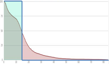
To explain the last point, Figure 1[left] shows the km curve for patients with stage-4 stomach cancer. Here, we can read off the claim that 50% of the patients will survive 11 months, and 95% will survive at least 2 months.111 In general, a survival curve is a plot where each point represents (the curve’s claim that) there is a chance of surviving at least time. Hence, in Figure 1[left], the [ 11 months, 50% ] point means this curve predicts a 50% chance of living at least 11 months (and hence a 10050 = 50% chance of dying within the first 11 months). The [ 2 months, 95% ] point means a 95% chance of surviving at least 2 months, and the [ 51 months, 5% ] point means a 5% chance of surviving at least 51 months. While these estimates do apply to the population, on average, they are not designed to be “accurate” for an individual patient since these estimates do not include patient-specific information such as age, treatments administered, or general health conditions. It would be better to directly, and correctly, incorporate these important factors explicitly in the prognostic models.
This heterogeneity of patients, coupled with the need to provide probabilistic estimates at several time points, has motivated the creation of several individual survival time distribution (isd) tools, each of which can use this wealth of healthcare information from earlier patients, to learn a more accurate prognostic model, which can then predict the isd of a novel patient based on all available patient-specific attributes. This paper considers several isd models: the Kalbfleisch-Prentice extension of the Cox (cox-kp) [29] and the elastic net Cox (coxen-kp) [55] model, the Accelerated Failure Time (aft) model [29], the Random Survival Forest model with Kaplan-Meier extensions (rsf-km), and the Multi-task Logistic Regression (mtlr) model [57]. Figure 1(middle, right) show survival curves (generated by mtlr) for two of these stage-4 stomach cancer patients, which incorporate other information about these individual patients, such as the patient’s age, gender, blood work, etc. We see that these prognoses are very different; in particular, mtlr predicts that [middle] Patient #1’s median survival time is 20.2 months, while [right] Patient #2’s is only 2.6 months. The blue vertical lines show the actual times of death; we see that each of these patients passed away very close to mtlr’s predictions of their respective median survival times.

One could then use such curves to make decisions about the individual patient. Of course, these decisions will only be helpful if the model is giving accurate information – i.e., only if it is appropriate to tell a patient that s/he has a 50% chance of dying before the median survival time of this predicted curve, and a 25% chance of dying before the time associated with the 25% on the curve, etc.
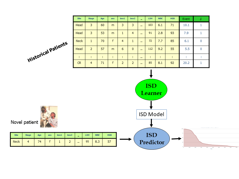
We focus on ways to learn such models from a “survival dataset” (see below), describing earlier individuals. Survival prediction is similar to regression as both involve learning a model that regresses the covariates of an individual to estimate the value of a dependent real-valued response variable – here, that variable is “time to event” (where the standard event is “death”). But survival prediction differs from the standard regression task as its response variable is not fully observed in all training instances – this task allows many of the instances to be “right censored”, in that we only see a lower bound of the response value. This might happen if a subject was alive when the study ended, meaning we only know that she lived at least (say) 5 years after the starting time, but do not know whether she actually lived 5 years and a day, or 30 years. This also happens if a subject drops out of a study, after say 2.3 years, and is then lost to follow-up; etc. Moreover, one cannot simply ignore such instances as it is common for many (or often, most) of the training instances to be right-censored; see Table 4. Such “partial label information” is problematic for standard regression techniques, which assume the label is completely specified for each training instance. Fortunately, there are survival prediction algorithms that can learn an effective model, from a cohort that includes such censored data. Each such “survival dataset” contains descriptions of a set of instances (e.g., patients), as well as two “labels” for each: one is the time, corresponding to the time from diagnosis to a final date (either death, or time of last follow-up) and the other is the status bit, which indicates whether the patient was alive at that final date. Section 2 summarizes several popular models for dealing with such survival data.
This paper provides three contributions: (1) Section 2 motivates the need for such isd models by showing how they differ from more standard survival analysis systems. (2) Section 3 then discusses several ways to evaluate such models, including standard measures (Concordance, 1-Calibration, Brier score), variants/extensions to familiar measures (L1-loss, Log-L1-loss), and also a novel approach, “D-Calibration” which can be used to assess the quality of the individual survival curves generated by isd models. (3) Section 4 evaluates several isd (and related) models (standard: km, cox-kp, aft and more recent: rsf-km, coxen-kp, mtlr) on 8 diverse survival datasets, in terms of all 5 evaluation measures. We will see that mtlr does well – typically outperforming the other models in the various measures, and often showing vast improvement in terms of calibration metrics.
The appendices provide relevant auxiliary information: Appendix A describes some important nuances about survival curves. Appendix B provides further details concerning all the evaluation metrics and in particular, how each addresses censored observations. It also contains some relevant proofs about our novel D-Calibration metric. Appendix C then explains some additional aspects of the isd models considered in this paper. Lastly, Appendix D gives the detailed results from empirical evaluation – e.g., providing detailed tables corresponding to the results shown as figures in Section 4.2.
For readers who want an introduction to survival analysis and prediction, we recommend Applied Survival Analysis by Hosmer and Lemeshow [26]. Wang et al. [51] surveyed machine learning techniques and evaluation metrics for survival analysis. However, that work primarily overviewed the standard survival analysis models, then briefly discussed some of the evaluation techniques and application areas. Our work, instead, focuses on the isd-based models – first motivating why they are relevant for survival prediction (with a focus on medical situations) then providing empirical results showing the strengths and weaknesses of each of the models considered.
2 Summary of Various Survival Analysis/Prediction Systems
There are many different survival analysis/prediction tools, designed to deal with various different tasks. We focus on tools that learn the model from a survival dataset,
| (1) |
which provides the values for features for each member of a cohort of historical patients, as well as the actual time of the “event” which is either death (uncensored) or the last visit (censored), and a bit that serves as the indicator for death.222 Throughout this work we focus on only Right-Censored survival data. Additionally, we constrain our work to the standard machine-learning framework, where our predictions are based only on information available at fixed time (e.g., start of treatment). While these descriptions all apply when dealing with the time to an arbitrary event, our descriptions will refer to “time to death”. See Figure 2, in the context of our isd framework.
Here, we assume is a vector of feature values describing a patients, using information that are available when that patient entered the study – e.g., when the patient was first diagnosed with the disease, or started the treatment. Additionally, we assume each patient has a death time, , and a censoring time, , and assign and where is the Indicator function – i.e., if or if . We follow the standard convention that and are assumed independent.
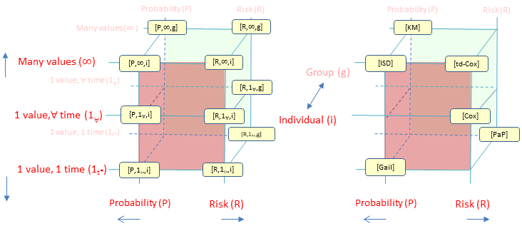
To help categorize the space of survival prediction systems, we consider 3 independent characteristics:
-
•
[R vs P] whether the system provides, for each patient, a risk score versus a probabilistic value (perhaps ).
-
•
[ vs vs ] whether the system returns a single value for each patient (associated either with a single time “” or with the overall survival “”), versus a range of values, one for each time. Here might refer to for a single time and if there is a single “atemporal” value (think of the standard risk score, which is not linked to a specific time), vs that refers to over all future times .
-
•
[i vs g] whether the result is “i ” specific to a single individual patient (i.e., based on a large number of features ) or is “g ” general to the population. This g also applies if the model deals with a fixed set of subpopulations – perhaps each contains all patients with certain values of only one or two features (e.g., subpopulation is all men under 50, are men over 50, and and are corresponding sets of women), or each subpopulation is a specified range of some computation (e.g., are those with BMI20, with BMI and , with BMI30).
This section summarizes 5 (of the ) classes of survival analysis tools (see Figure 3), giving typical uses of each, then discusses how they are interrelated.
2.1 [R,,i]: 1-value Individual Risk Models (cox)
An important class of survival analysis tools compute “risk” scores, for each patient , with the understanding that corresponds to predicting that will die before . Hence, this is a discriminative tool for comparing pairs of patients, or perhaps for “what if” analysis of a single patient (e.g., if he continues smoking, versus if he quits). These systems are typically evaluated using a discriminative measure, such as “Concordance” (discussed in Section 3.1). Notice these tools each return a single real value for each patient.
One standard generic tool here is the Cox Proportional Hazard (cox) model [10], which is used in a wide variety of applications. This models the hazard function333 The hazard function (also known as the failure rate, hazard rate, or force of mortality) is essentially the chance that will die at time , given that s/he has lived until this time, using the survival PDF . When continuous, . as
| (2) |
where are the learned weights for the features, and is the baseline hazard function. We view this as a Risk Model by ignoring (as is the same for all patients), and focusing on just . (But see the cox-kp model below, in [P,,i].) There are many other tools for predicting an individual’s risk score, typically with respect to some disease; see for example the Colditz-Rosner model [8], and the myriad of others appearing on the Disease Risk Index website444http://www.diseaseriskindex.harvard.edu/update/. For all of these models, the value returned is atemporal – i.e., it does not depend on a specific time. There are also tools that produce [R,,i] models, that return a risk score associated across all time point; see Section 3.1.
2.2 [R,,g]: Single-time Group Risk Predictors: Prognostic Scales (PPI, PaP)
Another class of risk predictions explicitly focus on a single time, leading to prognostic scales, some of which are computed using Likert scales [40]. For example, the Palliative Prognostic Index (PPI) [35] computes a risk score for each terminally ill patient, which is then used to assign that patient into one of three groups. It then uses statistics about each group to predict that patients in one group will do better at this specific time (here, 3 weeks), than those in another group. Similarly, the Palliative Prognostic Score (PaP) [38] uses a patient’s characteristics to assign him/her into one of 3 risk groups, which can be used to estimate the 30-day survival risk. (There are many other such prognostic scales, including [7, 2, 23].) Again, these tools are typically evaluated using Concordance.555 Here, they do not compare pairs of individuals from the same group, but only patients from different groups, whose events are comparable (given censoring); see Section 3.1.
2.3 [P,,i]: Single-time Individual Probabilistic Predictors (Gail, PredictDepression)
Another class of single-time predictors each produce a survival probability for each individual patient , for a single fixed time – which is the probability that will survive to at least time . For example, the Gail model [Gail] [9] 666http://www.cancer.gov/bcrisktool/ estimates the probability that a woman will develop breast cancer within 5 years based on her responses to a number of survey questions. Similarly, the PredictDepression system [PredDep] [50] 777http://predictingdepression.com/ predicts the probability that a patient will develop a major depressive episode in the next 4 years based on a small number of responses. The Apervite888https://apervita.com/community/clevelandclinic and R-calc999http://www.r-calc.com/ExistingFormulas.aspx?filter=CCQHS websites each include dozens of such tools, each predicting the survival probability for 1 (or perhaps 2) fixed time points, for certain classes of diseases.
Notice these probability values have semantic content, and are labels for individual patients (rather than risk-scores, which are only meaningful within the context of other patients’ risk scores). These systems should be evaluated using a calibration measure, such as 1-Calibration or Brier score (discussed in Sections 3.3 and 3.4).
2.4 [P,,g]: Group Survival Distribution (km)
There are many systems that can produce a survival distribution: a graph of , showing the survival probability for each time ; see Figure 1. The Kaplan-Meier analytic tool (km) is at the “class” level, producing a distribution designed to apply to everyone in a sub-population: , for every in some class – e.g., the km curve in Figure 1[left] applies to every patient with stage-4 stomach cancer. The SEER website101010http://seer.cancer.gov/ provides a set of Kaplan-Meier curves for various cancers. While patients can use such information to estimate their survival probabilities, the original goal of that analysis is to better understand the disease itself, perhaps by seeing whether some specific feature made a difference, or if a treatment was beneficial. For example, we could produce one curve for all stage-4 stomach cancer patients who had treatment tA, and another for the disjoint subset of patients who had no treatment; then run a log-rank test [22] to determine whether (on average) patients receiving treatment tA survived statistically longer than those who did not. Section 3 below describes various ways to evaluate [P,,i] models; we will use these measures to evaluate km models as well.
2.5 [P,,i]: Individual Survival Distribution, isd (cox-kp, coxen-kp, aft, rsf-km, mtlr)
The previous two subsections described two frameworks:
-
•
[P,,i] tools, which produce an individualized probability value , but only for a single time ; and
-
•
[P,,g] tools, which produce the entire survival probability curve for all points , but are not individuated – i.e., the same curve for all patients .
Here, we consider an important extension: a tool that produces the entire survival probability curve for all points , specific to each individual patient, . As noted in the previous section, this is required by any application that requires knowing meaningful survival probabilities for many time points. This model also allows us to compute other useful statistics, such as a specific patient’s expected survival time.
We call each such system an “Individual Survival Distribution” model, isd. While the Cox model is often used just to produce the risk score, it can be used as an isd, given an appropriate (learned) baseline hazard function ; see Equation 2. We estimate this using the Kalbfleisch-Prentice estimator [29], and call this combination “cox-kp”; we also consider a regularized Cox model, namely the elastic net Cox with the Kalbfleisch-Prentice extension (coxen-kp). We also explore three other models: Accelerated Failure Time model [29] with the Weibull distribution (aft), Random Survival Forests with the Kaplan-Meier extension (rsf-km, described in Appendix C.3) [28] and Multi-task Logistic Regression system (mtlr) [57]. Figure 4 shows the curves from these various models, each over the same set of individuals.

Above, we briefly mentioned three evaluation methods: Concordance, 1-Calibration, and Brier score. We show below that we can use any of these methods to evaluate a isd model. In addition, we can also use variants of “L1-loss”, to see how far a predicted single-time differs from the true time of death; see Section 3.2. Each of these 4 methods considers only a single time point of the distribution, or an average of scores, each based on only a single time, or a single statistic (such as its median value). We also consider a novel evaluation measure, “D-Calibration”, which uses the entire distribution of estimated survival probabilities; see Section 3.5.
2.6 Other Issues
The goal of many Survival Analysis tools is to identify relevant variables, which is different from our challenge here, of making a prediction about an individual. Some researchers use km to test whether a variable is relevant – e.g., they partition the data into two subsets, based on the value of that variable, then run km on each subset, and declare that variable to be relevant if a log-rank test claims these two curves are significantly different [22]. It is also a common use of the basic Cox model – in essence, by testing if the coefficient associated with feature (in Equation 2) is significantly different from 0 [48]. (We will later use this approach to select features, as a pre-processing step, before running the actual survival prediction model; see Section 4.1.)
Note this “g vs i ” distinction is not always crisp, as it depends on how many variables are involved – e.g., models that “describe” each instance using no variables (like km) are clearly “g ”, while models that use dozens or more variables, enough to distinguish each patient from one another, are clearly “i ”. But models that involve 2 or 3 variables typically will place each patient into one of a small number of “clusters”, and then assign the same values to each member of a cluster. By convention, we will catalog those models as “g ” as the decision is not intended to be at an individual level.
The “” vs “” distinction can be blurry, if considering a system that produces a small number of predictions for each individual – e.g., the Gail model provides a prediction of both 5 year and 25 year survival. We consider this system as a pair of “”-predictors, as those two models are different. (Technically, we could view them as “Gail[5year]” versus “Gail[25year]” models.)
Finally, recall there are two types of frameworks that each return a single value for each instance: the single value returned by the [R,,i]-model cox is atemporal – i.e., applies to the overall model – while each single value returned by the [P,,i]-model Gail and the [R,,g]-model PaP, is for a specific time, . (Note there can also be [P,,i]- and [R,,g]-models that are atemporal.)
2.7 Relationship of Distributional Models to Other Survival Analysis Systems
We will use the term “Distributional Model” to refer to algorithms within the [P,,g] and [P,,i] frameworks – i.e., both km and isd models. Note that such models can match the functionality of the first 3 “personalized” approaches. First, to emulate [P,,i], we just need to evaluate the distribution at the specified single time – i.e., . So for Patient #1 (from Figure 1), for “48 months”, this would be 20%. Second, to emulate [R,,i], we can just use the negative of this value as the time-dependent risk score – so the 4-year risk for Patient #1 would be -0.20. Third, to deal with [R,,i], we need to reduce the distribution to a single real number, where larger values indicate shorter survival times. A simple candidate is the individual distribution’s median value, which is where the survival curve crosses 50%.111111 Another candidate is the mean value of the distribution, which corresponds to the area under the survival curve; see Theorem B.1. So for Patient #1 in Figure 1, the median is 16 months. We can then view (the negative of) this scalar as the risk score for that patient. So for Patient #1, the “risk” would be . Fourth, to view the isd model in the [R,,g] framework, we need to place the patients into a small number of “relatively homogeneous” bins. Here, we could quantize the (predicted) mean value – e.g., mapping a patient to Bin#1 if that mean is in [0, 15), Bin#2 if in [15, 27), and Bin#3 if in [27, 70]. (Here, this patient would be assigned to Bin#2.) Fifth, to view the isd model in the [R,,g] framework, associated with a time , we could quantize the -probability – e.g., quantize the into 4 bins corresponding to the intervals [0, 0.20), [0.20, 0.57), [0.57, 0.83], and [0.83, 1.0].
These simple arguments show that a distributional model can produce the scalars used by five other frameworks [P,,i], [R,,i], [R,,i], [R,,g], and [R,,g]. Of course, a distributional model can also provide other information about the patient – not just the probability associated with one or two time points, but at essentially any time in the future, as well as the mean/median value. Another advantage of having such survival curves is visualization (see Figure 1): it allows the user (patient or clinician) to see the shape of the curve, which provides more information than simply knowing the median, or the chance of surviving 5 years, etc.
There are some subtle issued related to producing meaningful survival curves – e.g., many curves end at a non-zero value: note the km curve in Figure 4(top left) stops at (83, 0.12), rather than continue to intersect the x-axis at, perhaps (103, 0.0). This is true for many of the curves produced by the isds. Indeed, some of the curves do not even cross , which means the median time is not well-defined; cf. the top orange line on the aft curve (top right), which stops at (83, 0.65), as well as many of the other curves throughout that figure. This causes many problems, in both interpreting and evaluating isd models. Appendix A shows how we address this.
3 Measures for Evaluating Survival Analysis/Prediction Models
The previous section mentioned 5 ways to evaluate a survival analysis/prediction model: Concordance, 1-Calibration, Brier score, L1-loss, and D-Calibration. This section will describe these – quickly summarizing the first four (standard) evaluation measures (and leaving the details, including discussion of censoring, for Appendix B) then providing a more thorough motivation and description of the fifth, D-Calibration. The next section shows how the 6 distribution-learning models perform with respect to these evaluations.
For notation, we will assume models were trained on a training dataset, formed from the same triples as shown in Equation 1, that is where is the set of uncensored instances (notice the event time, , here is written as ), and is the set of censored instances (, here is written as ). Note also that this training dataset is disjoint from the validation dataset, . Since models are evaluated on and we save discussion of censoring for Appendix B, we assume here that all of is uncensored – i.e., (to simplify notation).
3.1 Concordance
As noted above, each individual risk model [R,,-] (i.e., [R,,i] or [R,,g], where can be either or ) assigns to each individual , a “risk score” , where means the model is predicting that will die before . Concordance (a.k.a. C-statistic, C-index) is commonly used to validate such risk models. Specifically, Concordance considers each pair of patients, and asks whether the predictor’s values for those patients matches what actually happened to them. In particular, if the model gives a higher score than , then the model gets 1 point if dies before . If instead died before , the model gets 0 points for this pair. Concordance computes this for all pairs of comparable patients, and returns the average.
When considering only uncensored patients, every pair is comparable, which means there are pairs from elements. Given these comparable pairs, Concordance is calculated as,
| (3) |
As an example, consider the table of death times and risk scores, for 5 patients, shown in Table 1[left]. Table 1[right] shows that these risk scores are correct in 7 of the pairs, so the Concordance here is 7/10 = 0.7.
| Id | Riski | |
|---|---|---|
| 1 | 1 | 6 |
| 2 | 3 | 3 |
| 3 | 4 | 5 |
| 4 | 6 | 2 |
| 5 | 9 | 4 |
| 1 | 2 | 3 | 4 | 5 | |
|---|---|---|---|---|---|
| 1 | |||||
| 2 | + | ||||
| 3 | + | 0 | |||
| 4 | + | + | + | ||
| 5 | + | 0 | + | 0 |
This Concordance measure is very similar to the area under the receiver operating curve (AUC) and equivalent when is constrained to values {0, 1} [33].
This Concordance measure is relevant when the goal is to rank or discriminate between patients – e.g., when one wants to know who will live longer between a pair of patients. (For example, if we want to transplant an available liver to the patient who will die first – this corresponds to “urgency”.) Concordance is the desired metric here due to it’s interpretation, i.e. given two randomly selected patients, and , if a model with Concordance of 0.9 assigns a higher risk score to than , then there is a 90% chance that will die before .
While [R,,i] models (such as cox) provide a risk score that is independent of time, there are also [R,,i] models that produces a risk score for an instance that depends on time ; such as Aalen’s additive regression model [1] or time-dependent Cox (td-Cox) [14], which uses time-dependent features. These models can be evaluated using time-dependent Concordance (aka, “time-dependent ROC curve analysis”) [24].
Finally, the [R,,g] systems compute a risk score, but then bin these scores into a small set of intervals. When computing Concordance, they then only consider patients in different bins. For example, if Bin1 = [0, 10] and Bin2 = [11, 20], then this evaluation would only consider pairs of patients where one is in Bin1 and the other is in Bin2 – e.g., and . (Hence, it will not consider the pair if both .)
See Appendix B.1 for more details, including a discussion of how this measure deals with censored instances and tied risk scores/death times.
3.2 L1-loss
Survival prediction is very similar to regression: given a description of a patient, predict a real number (his/her time of death). With this similarity in mind, one can evaluate a survival model using the techniques used to evaluate regression tasks, such as L1-loss – the average absolute value of the difference between the true time of death, , and the predicted time : . (We consider the L1-loss, rather than L2-loss which squares the differences, as the distribution of survival times is often right skewed, and L1-loss is less swayed by outliers than L2-loss.)
One challenge in applying this measure to our [P,,-] models is identifying the predicted time, . Here, we will use the predicted median survival time, that is , leading to the following measure:
| (4) |
While we would like this value to be small, we should not expect it to be 0: if the distribution is meaningful, there should be a non-zero chance of dying at other times as well. For example, while the L1-loss is 0 for the Heaviside distribution at the time of death (shown in green in Figure 5), this is unrealistic.
Appendix B.2 discusses many issues with the L1-loss measure, related to censored data, and reasons to consider using the of survival time.
3.3 1-Calibration
The [P,,i] tools estimate the survival probability for each instance , at a single time point . For example, the PredictDepression system [50] predicts the chance that a patient will have a major depression episode within the next 4 years, based on their current characteristics – i.e., this tool produces a single probability value for each patient described as . We can use 1-Calibration to measure the effectiveness of such predictors. To help explain this measure, consider the “weatherman task” of predicting, on day , whether it will rain on day . Given the uncertainty, forecasters provide probabilities. Imagine, for example, there were 10 times that the weatherman, Mr.W, predicted that there was a 30% chance that it would rain tomorrow. Here, if Mr.W was calibrated, we expect that it would rain 3 of these 10 times – i.e., 30%. Similarly, of the 20 times Mr.W claims that there is an 80% chance of rain tomorrow, we expect rain to occur 16 = 20 0.8 of the 20 times.
Here, we have described a binary probabilistic prediction problem – i.e., predicting the chance that it will rain the next day. One of the most common calibration measures for such binary prediction problems is the Hosmer-Lemeshow goodness-of-fit test [25]. First, we sort the predicted probabilities for this time for all patients and group them into a number () of “bins”; commonly into deciles, i.e., bins. Suppose there are 200 patients; the first bin would include the 20 patients with the largest values, the second bin would contain the patients with the next highest set of values, and so on, for all 10 bins. Next, within each bin, we calculate the expected number of events, . We also let be the size of the bin (here, ), and be the number of patients (in the bin) who died before . Recalling that denotes Patient #i’s time of death and letting denote the event status of the patient at : for the th bin, , we have . Figure 6 graphs the 10 values of observed and expected for the deciles, for two different tests (corresponding to two different isd-models, on the same dataset and time). Additionally, see Appendix B.3 for an example walking through 1-Calibration.
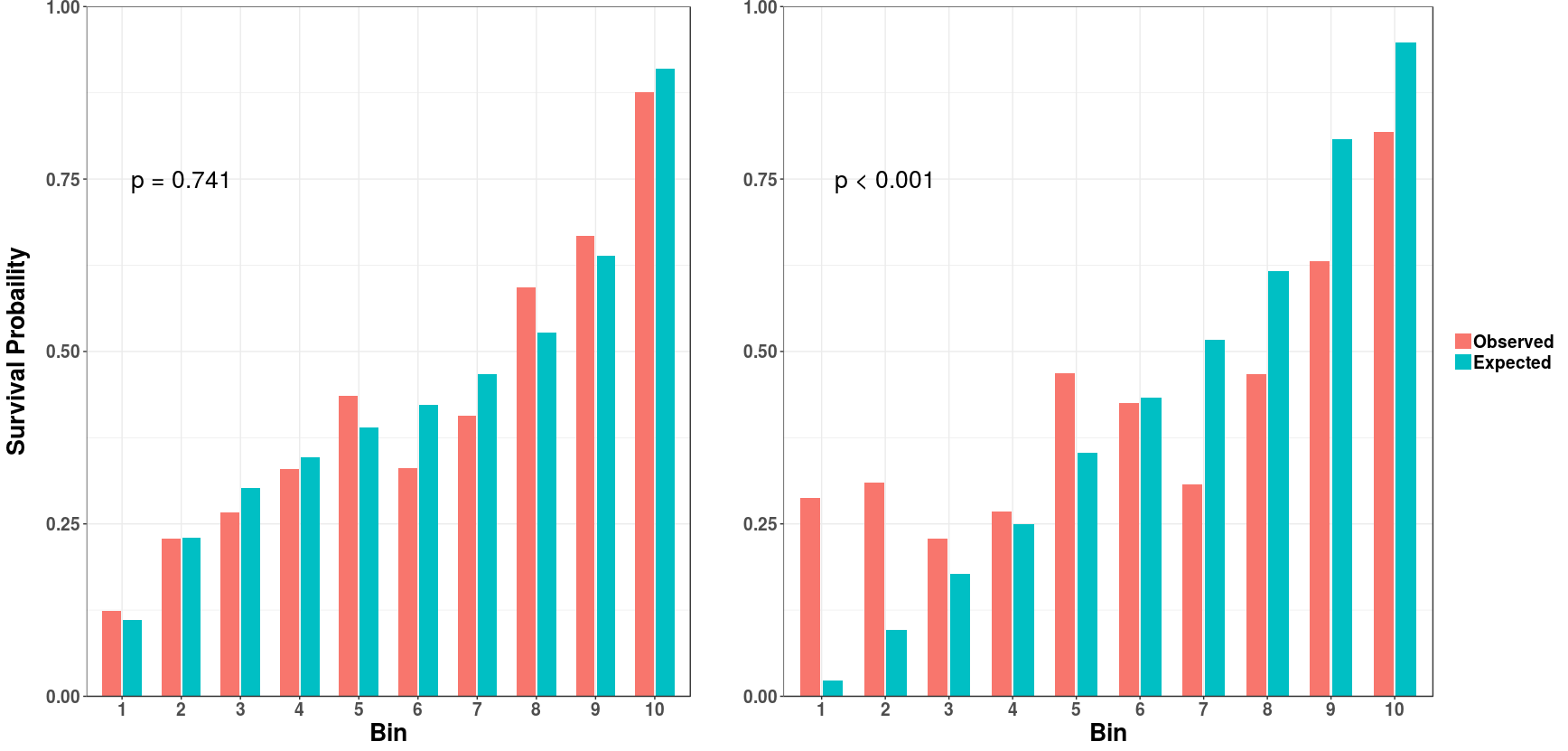
For each test, we can then compute the Hosmer-Lemeshow test statistic:
If the model is 1-Calibrated, then this statistic follows a distribution, which then can be used to find a -value. For a given time , finding suggests the survival model is not well calibrated at – i.e., the predicted probabilities of survival at may not be representative of patient’s true survival probability at .
Returning to Figure 6, the HL statistics are 5.99 and 321.44, for the left and right, leading to the -values 0.741 and 0.001 – meaning the left one passes but the right one does not. (This is not surprising, given that each pair of bars on the left are roughly the same height, while the pairs of the right are not.)
Note that a [P,,i] model, which gives probabilities for multiple time points, may be calibrated at one time , but not be calibrated at another time , since , and are dependent on the chosen time point. This issue motivated us to define a notion of calibration across a distribution of time points, D-Calibration, in Section 3.5. Appendix B.3 provides further details about 1-Calibration including ways to handle censored patients.
3.4 Brier Score
We often want a model to be both discriminative (high Concordance) and calibrated (passes the 1-Calibration test). While one can rank Concordance scores to compare two models’ discriminative abilities, 1-Calibration cannot rank models besides suggesting one model is calibrated ( and one is not (as -values are not intended to be ranked). The Brier score [6] is a commonly used metric that measures both calibration and discrimination; see Appendix B.4.1. Mathematically, the Brier score is the mean squared error between the {0, 1} event status at time and the predicted survival probability at . Given a fully uncensored validation set , the Brier score, at time , is
| (5) |
Here, a perfect model (that only predicts 1s and 0s as survival probabilities and is correct in every case) will get the perfect score of 0, whereas a reference model that gives for all patients will get a score of 0.25.
An extension of the Brier score to an interval of time points is the Integrated Brier score, which will give an average Brier score across a time interval,
| (6) |
We will use this measure for our analysis, where is the maximum event time of the combined training and validation datasets – this way, the interval evaluated is equivalent across cross-validation folds.
As noted above, the Brier score measures both calibration and discrimination, implying it should be used when seeking a model that must perform well on both calibration and discrimination, or when one is investigating the overall performance of survival models. Appendix B.4 shows how to incorporate censoring into the Brier score, and discusses the decomposition of the Brier score into calibration and discriminative components.
3.5 D-Calibration
The previous sections summarized several common ways to evaluate standard survival prediction models, that produce only a single value for each patient – e.g., the patient’s risk score, perhaps with respect to a single time, or the mean survival time. (Each is a [-,,-] model.) However, the [P,,-] tools produce a distribution – i.e., each is a function that maps to (with some constraints of course), such as the ones shown in Figure 4; see Footnote 1. It would be useful to have a measure that examines the entire distribution as a distribution.121212While the Integrated Brier score does consider all the points across the distribution, it simply views that distribution as a set of points; see Appendix B.4.2 for further explanation.
A distributional calibration (D-Calibration) [3] measure addresses the critical question:
| Should the patient believe the predictions implied by the survival curve? | (7) |
First, consider population-based models [P,,g], like Kaplan-Meier curves – e.g., Figure 1[left], for patients with stage-4 stomach cancer. If a patient has stage-4 stomach cancer, should s/he believe that his/her median survival time is 11 months, and that s/he has a 75% chance of surviving more than 4 months? To test this, we could take 1000 new patients (with stage-4 stomach cancer) and ask whether 500 of these patients lived at least 11 months, and if 750 lived more than 4 months.
For notation, given a dataset, , and [P,,g]-model , and any interval , let
| (8) |
be the subset of (uncensored) patients in whose time of death is assigned a probability (by ) in the interval . For example, is the subset of patients who lived at least the median survival time (using ’s median), and is the subset who died after the 25th percentile of . By the argument above, we expect to contain about 1/2 of , and to contain about 3/4 of . Indeed, for any interval , we expect
| (9) |
or in general
| (10) |
This leads to the idea of a survival distribution [P,,g] model, , being D-Calibrated: For each uncensored patient , we can observe when s/he died , and also determine the percentile for that time, based on : . If is D-Calibrated, we expect roughly 10% of the patients to die in the [90%, 100%] interval – i.e., – and another 10% to die in the [80%, 90%) interval, and so forth for each of the 10 different 10%-intervals. More precisely, the set over all of the patients should be distributed uniformly on , which means that each of the 10 bins would contain 10% of .
This suggests a measure to evaluate a distributional model: see how close each of these 10 bins is to the expected 10%. We therefore use Pearson’s test: compute the -statistic with respect to the ten 10% intervals, and ask whether the bins appear uniform, at (say) the 0.05 level. Theorem B.2 (in Appendix B.5) states and proves the appropriateness of the Pearson’s goodness-of-fit test.
This addresses the question posed at the start of this subsection (Equation 7):
| Yes, a patient should believe the prediction from the survival curve | ||
| whenever this goodness-of-fit test reports . |
3.5.1 Dealing with Individual Survival Distributions, isd
Everything above was for a population-based distributional model [P,,g]. These specific results do not apply to individual survival distributions [P,,i]: For example, consider a single patient, Patient #1, whose curve is shown in Figure 1[middle]. Should he believe this plot, which implies that his median survival time is 18 months, and that he has a 75% chance of surviving more than 13 months?
If we could observe 1000 patients exactly identical to this Patient #1, we could verify this claim by seeing their actual survival times: this survival curve is meaningful if its predictions matched the outcomes of those copies – e.g., if around 250 died in the first 13 months, another 250 in months 13 to 18, etc.
Unfortunately, however, we do not have 1000 “copies” of Patient #1. But here we do have many other patients, each with his/her own characteristic survival curve, including the 4 curves shown in Figure 7. Notice each patient has his/her own distribution, and hence his/her own quartiles – e.g., the predicted median survival times for Patient A (resp., B, C and D), are 28.6 (resp., 65.7, 11.4, and 13.9) months; see Table 2. For these historical patients, we know the actual event time for each.131313 Here we just consider uncensored patients; Appendix B.5 extends this to deal with censoring. Here, if our predictor is working correctly, we would expect that 2 of these 4 would pass away before respective median times, and the other 2 after their median times. Indeed, we would actually expect 1 to die in each of the 4 quartiles; the blue vertical lines (the actual times of death) show that, in fact, this does happen. See also Table 2.
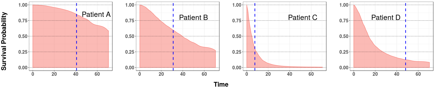
| Patient ID | Median Survival Time | Event time | Event Percentage | Quartile |
|---|---|---|---|---|
| A | 85.5 | 43.4 | 84.7 | #1 |
| B | 39.6 | 31.1 | 59.8 | #2 |
| C | 4.7 | 7.5 | 30.4 | #3 |
| D | 13.9 | 48.3 | 12.8 | #4 |
With a slight extension to the earlier notation (Equation 8), for a dataset and [P,,i]-model , and any interval , let
| (11) |
be the subset of (uncensored) patients in the dataset whose time of death is assigned a probability (based on its individual distribution, computed by ) in the interval .
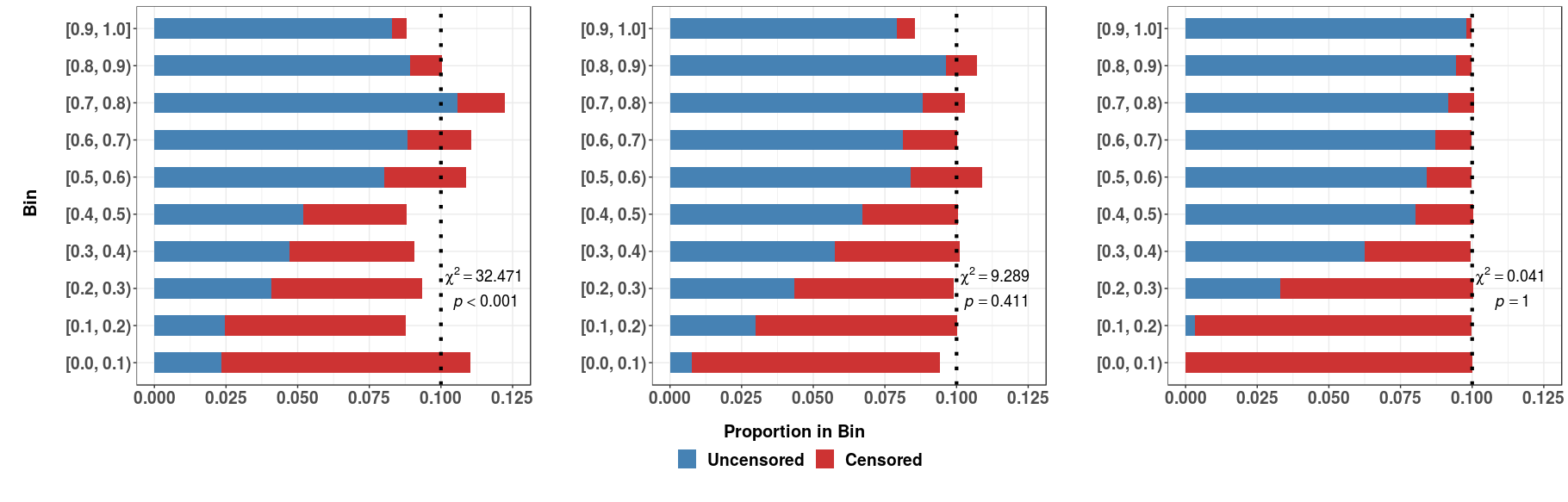
As above, we could put these into “10%-bins”, and then ask if each bin holds about 10% of the patients. The right-side of Figure 8 plots that information, for the isd learned by mtlr from the NACD dataset (described in Section 4.1), as a sideways histogram. We see that each of these intervals is very close to 10%. In fact, the goodness-of-fit test yields 0.433, which suggests that this isd is sufficiently uniform that we can believe that these survival curves are D-calibrated.
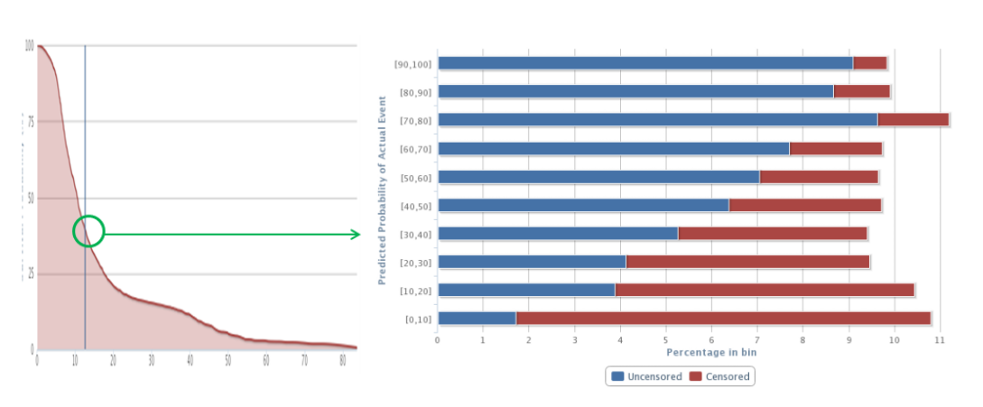
Note that Figure 8 is actually showing 5-fold cross-validation results: the survival curve for each patient was computed based on the model learned from the other 4/5 of the data, which is then applied to this patient [53]. Also, the rust-colored intervals correspond to the censored patients; see Appendix B.5 for an explanation.
3.5.2 Relating D-Calibration to 1-Calibration
This standard notion of 1-Calibration is very similar to D-Calibration, as both involve binning probability values and applying a goodness-of-fit test. However, 1-Calibration involves a single prediction time – here , which is the probability that the patient will survive at least to the specified time, . Patients are then sorted by these probabilities, partitioned into equal-size bins, and assessed as to whether the observed survival rates for each bin match the predicted rates using a Hosmer-Lemeshow test. By contrast, D-Calibration considers the entire curve, over all times – producing curves like the ones shown in Figures 1, 4, and 7. Each curve corresponds to a patient, who has an associated time of death, . Here, we are considering the model’s (estimated) probability of the patient’s survival at his/her time of death, given by . These patients are then placed into bins,141414Note the number of bins does not have to be 10 – we chose 10 to match the typical value chosen for the 1-Calibration test. based on the values of their associated probabilities, . Here the goodness-of-fit test measures whether the resulting bins are approximately equal-sized, as would be expected if accurately estimated the true survival curves (argued further in Appendix B.5).
Note D-Calibration tests the proportion of instances in bins across the entire interval, but this is not required for the “single probability” 1-Calibration. For example, the single probability estimates for the rsf-km curve in Figure 3, at time 20, range only from 0.05 to 0.62. That is, the distribution calibration should match the uniform distribution over [0,1], while the single probability calibration is instead expected to match the empirical percentage of deaths.
Table 3 summarizes the differences between D-Calibration and 1-Calibration.151515Further differences occur when considering how censored patients are handled; see Appendices B.3 and B.5. To see that they are different, Proposition B.3, in Appendix B.5, gives a simple example of a model that is perfectly D-Calibrated but clearly not 1-Calibrated, and another example that is perfectly 1-Calibrated but clearly not D-Calibrated. In addition, we will see below several examples of this – e.g., coxen-kp is D-Calibrated for the GLI dataset, but it is not 1-Calibrated at any of the 5 time points considered, and aft is 1-Calibrated for the 50th and 75th percentiles of GBM but is not D-Calibrated.
| 1-Calibration | D-Calibration | |
|---|---|---|
| Objective | Evaluate Single Time Probabilities | Evaluate Entire Survival Curve |
| Values considered | ||
| Should match | Empirical number of deaths | Uniform |
| Statistical Test | Hosmer-Lemeshow test | Pearson’s test |
4 Evaluating isd Models
Sections 2.4 and 2.5 listed several distributional models (km, and the isds: cox-kp, coxen-kp, aft, mtlr, and rsf-km), and Section 3 provided 5 different evaluation measures: Concordance, L1-loss, 1-Calibration, Integrated Brier score, and D-Calibration. This section provides an empirical comparison of these 6 models, with respect to all 5 of these measures, over 8 datasets.
Of course, these 6 models do not include all possible survival models; they instead serve as a sample of the types of models available. The km, cox-kp, and aft model are all very common – these are standard approaches used throughout survival analysis and represent non-parametric, semi-parametric, and parametric models, respectively. As our preliminary studies with cox-kp suggested it was overfitting, we also included a regularized extension, using elastic net, coxen-kp. Since Random Survival Forests (rsf) were introduced in 2008, they have had a large impact on the survival analysis community. However, as the Kaplan-Meier extension to transform rsf into an isd is not well known, it is summarized in Appendix C.3. More recent still is the mtlr technique [57] that directly learns a survival distribution, by essentially learning the associated probability mass function (whose sequential right-to-left sum, when smoothed, is the survival distribution). We found some subsequent similar models, including “Multi-Task Learning for Survival Analysis” (MTLSA) [33], some deep learning variants [39, 32, 34], and a computationally demanding Bayesian regression trees model [44], but for brevity, we focused on just the first such model, mtlr.
Note the distribution class chosen for aft certainly influences its performance – e.g., it is possible that aft[Weibull] on a dataset may fail D-Calibration whereas aft[Log-Logistic] may pass; similarly for 1-Calibration at some time , and the scores for Concordance, L1-loss and Integrated Brier score will depend on that distribution class. This paper will focus on aft[Weibull] because, while still being parametric, the Weibull distribution is versatile enough to fit many datasets.
4.1 Datasets and Evaluation Methodology
There are many different survival datasets; here, we selected 8 publicly available medical datasets in order to cover a wide range of sample sizes, number of features, and proportions of censored patients. We excluded small datasets (with fewer than 150 instances) to reduce the variance in the evaluation metrics. Our datasets ranged from 170 to 2402 patients, from 12 to 7401 features, and percentage of censoring from 17.23% to 86.21%; see Table 4. Note that we have not included extremely high-dimensional data (with tens of thousands of features, often found in genomic datasets), as such data raises additional challenges beyond the scope of standard survival analysis; see [52] for methods to handle extremely high-dimensional data.
The Northern Alberta Cancer Dataset (NACD), with 2402 patients and 53 features, is a conglomerate of many different cancer patients, including lung, colorectal, head and neck, esophagus, stomach, and other cancers. In addition to using the complete NACD dataset, we considered the subset of 950 patients with colorectal cancer (Nacd-Col), with the same 53 features.
Another four datasets were retrieved from data generated by The Cancer Genome Atlas (TCGA) Research Network [15]: Glioblastoma multiforme (GBM; 592 patients, 12 features), Glioma (GLI; 1105 patients, 13 features), Rectum adenocarcinoma (READ; 170 patients, 18 features), and Breast invasive carcinoma (BRCA; 1095 patients, 61 features). To ensure a variety of feature/sample-size ratios, we consider only the clinical features in our experiments.
Lastly, we included two high-dimensional datasets: the Dutch Breast Cancer Dataset (DBCD) [49] contains 4919 microarray gene expression levels for 295 women with breast cancer, and the Diffuse Large B-Cell Lymphoma (DLBCL) [33] dataset contains 7401 features focusing on Lymphochip DNA microarrays for 240 biopsy samples.
We applied the following pre-processing steps to each dataset: We first removed any feature that was missing over 25% of its values, as well as any features containing only 1 unique value. For the remaining features, we “one-hot encoded” each nominal feature and then passed each feature to a univariate Cox filter, and removed any feature that was not significant at the level. Following feature selection, we replaced any missing value with the respective feature’s mean value. (Note this feature selection was found to benefit all isd models across all performance metrics; data not shown.) Table 4 provides the dataset statistics and a full breakdown of feature numbers in each step.
| GBM | GLI | Nacd-Col | NACD | READ | BRCA | DBCD | DLBCL | ||
| Number of patients: | 592 | 1105 | 950 | 2402 | 170 | 1095 | 295 | 240 | |
| % Censored | 17.23 | 44.34 | 51.89 | 36.59 | 84.12 | 86.21 | 73.22 | 42.50 | |
| # Features Originally: | 12 | 13 | 53 | 53 | 18 | 61 | 4921 | 7401 | |
| # Features Post-Processing: | 9 | 10 | 45 | 53 | 13 | 59 | 4921 | 7401 | |
| # Features Selected: | 6 | 10 | 34 | 46 | 8 | 28 | 2330 | 1771 | |
| 0.010 | 0.009 | 0.036 | 0.019 | 0.047 | 0.026 | 7.898 | 7.379 |
Following feature selection, features were normalized (transformed to zero mean with unit variance) and passed to models for five-fold cross validation (5CV). We compute the folds by sorting the instances by time and censorship, then placing each censored (resp., uncensored) instance sequentially into the folds – meaning all folds had roughly the same distribution of times, and censorships.
For coxen-kp, rsf-km, and mtlr we used an internal 5CV for hyper-parameter selection. There were no hyper-parameters to tune for the remaining models: cox, km, and aft.
As 1-Calibration required specific time points, and as models might perform well on some survival times but poorly on others, we chose five times to assess the calibration results of each model: the 10th, 25th, 50th, 75th, and 90th percentiles of survival times for each dataset. Here, we used the D’Agostino-Nam translation to include censored patients for these evaluation results – see Appendix B.3. Appendix D.4 presents all 240 values (6 models 8 datasets 5 time-points); here we instead summarize the number of datasets that each model passed as 1-Calibrated (at 0.05) for each percentile.
For all evaluations, we report the averaged 5CV results for Concordance, Integrated Brier score, and L1-loss. As Concordance requires a risk score, we use the negative of the median survival time and similarly use the median survival time for predictions for the L1-loss. To adjust for presence of censored data, we used the L1-Margin loss, given in Appendix B.2, which extends the “Uncensored L1-loss” given in Section 3.2 (which considers only uncensored patients). Additionally, as 1-Calibration (resp., D-Calibration) results are reported as -values, and it is not appropriate to average over the folds, we combined the predicted survival curves from all cross-validation folds for a single evaluation, and report the resulting -value.
Empirical evaluations were completed in R version 3.4.4. The implementations of km, aft, and cox-kp can all be found in the survival package [47] whereas coxen-kp uses the cocktail function found in the fastcox package [56]. Both rsf and rsf-km come from the randomForestSRC package [27]. An implementation of mtlr (and of all the code used in this analysis) is publicly available on the GitHub account161616https://github.com/haiderstats/ISDEvaluation of the lead author.
4.2 Empirical Results
Below, we consider a dataset to be “Nice” if its feature-to-sample-size ratio was less than 0.05 (for the final feature set) and its censoring was less than 55%; this includes four of the 8 datasets: GBM, Nacd-Col, GLI, NACD – which are shown first in all of our empirical studies. We let “High-Censor” datasets refer to READ and BRCA and “High-Dimensional” datasets refer to the other two (DLBCL and DBCD).
4.2.1 Concordance, Integrated Brier score, and L1-loss Results
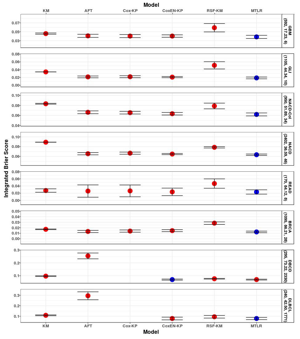
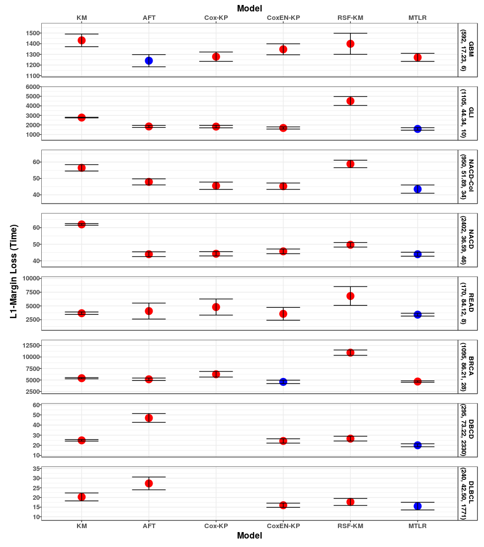
Figures 9, 10 and 11 give the empirical results for Concordance, Integrated Brier score, and L1-Margin loss respectively, where each circle is the score of the associated model on the dataset, and lines correspond to one standard deviation (over the 5 cross-validation folds). Appendix D provides the exact empirical results for these measures.
Best Performance: The blue circles represent the best performing models, for each dataset; here we find that mtlr performs best on a majority of datasets: six of eight for Concordance and L1-loss, and seven of eight for the Integrated Brier score.
Nice Datasets: Recall that the first 4 datasets are Nice. Here, we find that most models performed comparably – and in particular, aft and cox-kp perform nearly as well as the other, more complex, models. aft even performs best in terms of L1-loss on GBM. The only exception was rsf-km, which did much worse on GBM and GLI, in all three measures.
km was worse than the various isd-models for all 3 measures. (The only exception was rsf-km, which was worse on for the datasets GLI and GBM for Integrated Brier score, and for those datasets and also Nacd-Col for L1-loss.)
High-Censor Datasets – READ and BRCA: Note first that the variance in the evaluation metrics is generally higher on READ for all models (except km) due to the small number of uncensored patients within each test fold – this is not present in BRCA due to the larger sample size (1095). Again we find that coxen-kpand mtlr are similar for all three measures, but rsf-km performs consistently worse across all three metrics for both READ and BRCA. aft and cox-kp are either comparable (or inferior) to the other three isd-models: Concordance: worse performance but within error-bars for READ and BRCA; Integrated Brier score: similar for both READ and BRCA; L1-loss: slightly worse for READ and BRCA. Additionally, aft and cox-kp tend to show higher variance in evaluation estimates on READ than other models for all three measures.
km is worse than all 5 isd-models for Concordance, but comparable to the best for Integrated Brier score and L1-loss (actually scoring better than cox-kp and aft for L1-loss on READ and beating cox-kp on BRCA).
High-Dimensional Datasets – DBCD and DLBCL: There are no entries for cox-kp for these two datasets as it failed to run on them, likely due to the large number of features. As aft is unregularized, it is not surprising that it does poorly across all measures for these high-dimensional datasets – indeed, even worse than km, which did not use any features! We see that the other three isd-models – coxen-kp, mtlr and rsf-km – perform similarly to one another here, and km also achieves similar results (ignoring Concordance where km always achieves 0.5, as it gives identical predictions for all patients).

| 10th | 25th | 50th | 75th | 90th | |
|---|---|---|---|---|---|
| aft | 4 | 2 | 1 | 1 | 0 |
| cox-kp | 4 | 2 | 2 | 1 | 0 |
| coxen-kp | 4 | 3 | 1 | 2 | 2 |
| rsf-km | 4 | 2 | 2 | 1 | 0 |
| mtlr | 6 | 8 | 6 | 3 | 4 |
4.2.2 1-Calibration Results
Table 5 gives the number of datasets each model passed for 1-Calibration for each time of interest. We see that mtlr is typically 1-Calibrated across the percentiles of survival times. Specifically, mtlr is 1-Calibrated for at a minimum of four of eight datasets for the 10th, 25th, 50th, and 90th percentiles, outperforming all other models considered. The 90th percentile appear to be the most challenging in general, as some models (aft, cox-kp, rsf-km) are not 1-Calibrated for any datasets, coxen-kp is 1-Calibrated for two, and mtlr is 1-Calibrated for four. The 75th percentile also showed to be challenging, however aft, cox-kp, and rsf-km were 1-Calibrated for one, coxen-kp is 1-Calibrated for two, and mtlr is 1-Calibrated for three. The most challenging datasets for rsf-km once again were GBM, GLI, BRCA, and READ, for which rsf-km was 1-Calibrated only at the 10th percentile for READ – see Appendix D.4. Additional challenging datasets include the complete NACD and DBCD which were challenging for all models. As km assigns an identical prediction for all patients, it cannot partition patients into different bins, meaning it cannot be evaluated by 1-Calibration.
4.2.3 D-Calibration Results
Table 6, which gives the D-Calibration -values for each model and dataset, shows that both km and mtlr pass D-Calibration for every dataset, with km receiving the highest possible -value, 1.000, for each. (In fact, Lemma 2 in Appendix B.5 proves that km is asymptotically D-Calibrated). While km will tend to be D-Calibrated, it is also the least informative model, since it assigns all patients the same survival curve. mtlr is also D-Calibrated for all datasets, but in addition, it also provides each patients with his/her own survival curve.
Following km and mtlr, coxen-kp performed next best, only failing to be D-Calibrated for one dataset: NACD. rsf-km followed closely behind, being D-Calibrated for five of eight datasets, failing on GBM, GLI, and NACD. aft performed similarly to cox-kp, each of which being D-Calibrated on three of eight datasets.
Figure 12 provides (sideways) histograms, to help visualize D-calibration. For each subfigure, each of the 10 horizontal bars should be 10%; we see a great deal of variance for the not-D-Calibrated cox-kp [left], a small (but acceptable) variability for the D-Calibrated mtlr [middle], and essentially perfect alignment for the D-Calibrated km [right]. See also Figure 8.
| GBM | GLI | Nacd-Col | NACD | READ | BRCA | DBCD | DLBCL | Total | ||
|---|---|---|---|---|---|---|---|---|---|---|
| km | 1.000 | 1.000 | 1.000 | 1.000 | 1.000 | 1.000 | 1.000 | 1.000 | 8 | |
| aft | 0.000 | 0.017 | 0.290 | 0.000 | 0.807 | 0.988 | 0.000 | 0.000 | 3 | |
| cox-kp | 0.046 | 0.049 | 0.107 | 0.000 | 0.939 | 0.995 | - | - | 3 | |
| coxen-kp | 0.447 | 0.128 | 0.691 | 0.000 | 1.000 | 1.000 | 0.430 | 0.758 | 7 | |
| rsf-km | 0.000 | 0.000 | 0.403 | 0.000 | 0.974 | 0.757 | 0.911 | 0.574 | 5 | |
| mtlr | 0.688 | 0.883 | 0.656 | 0.411 | 1.000 | 0.995 | 0.994 | 0.755 | 8 |
5 Discussion
Comparing different isd-models: Steyerberg et al. [46] noted two different types of performance measures of a survival analysis model – calibration and discrimination – each of which can be assessed separately:
- Calibration:
-
“Of 100 patients with a risk prediction of %, do close to experience the event?”
- Discrimination:
-
“Do patients with higher risk predictions experience the event sooner than those who have lower risk predictions?”
Discrimination is a very important measure for some situations – e.g., if we have 2 patients who each need a kidney transplant, but there is only a single kidney donor, then we want to know which patient will die faster without the transplant [30]. As discussed in Section 3.1, Concordance measures how well a predictor does, in terms of this discrimination task.
This paper, however, motivates and studies models that produce an individual survival curve for a specific patient. Such isd tools may not be optimal for maximizing discrimination (and therefore Concordance); and even tools like cox and rsf, that were originally developed for discrimination, were then extended to produce these individual survival curves. Given this qualifier, we see (over the set of isd tools tested), mtlr scored best on Concordance for six of the eight datasets tested and rsf-km scored the best on the other two. (The relatively low performance of cox-kp is unexpected given the claim that “a method designed to maximize the Cox’s partial likelihood also ends up (approximately) maximizing the [concordance]” [45].) However, when we look at the Nice datasets, 4 of the 5 isd-models give nearly identical results (rsf-km differs by giving noticeably lower performance on GBM and GLI). These findings suggest that, for Nice datasets, more complex models (mtlr, rsf-km, and coxen-kp) do not offer large benefits in terms of Concordance. For the High-Dimensional datasets, mtlr and coxen-kp performed only marginally better than rsf-km for DBCD but noticeably better than rsf-km on DLBCL. Although these are only two datasets, this suggests that rsf-km may not be optimal for these high-dimensional datasets, in terms of Concordance. For the High-Censor datasets rsf-km saw much worse performance for Concordance (among other metrics) suggesting rsf-km may not be suitable for datasets with a high proportion of censored data.
As noted above, Concordance is only one measure for an isd tool. Given that an isd tool can produce a survival curve for each patient (and not just a single real-valued score), it can be used for various tasks, with various associated evaluations. For example, consider patients who are deciding whether to undergo an intensive medical procedure. Using the plots from Figure 7, note that Patient C has a very steep survival curve with a low median survival time, while Patient A has a shallow survival curve with a large median survival time. If we were to use this to predict the outcome of a procedure, we might expect Patient C to opt-out of the procedure, but Patient A to go through with it. Note the decision for Patient C is completely independent of Patient A, in that we could give the procedure to one, both, or neither of them. As these patients are not being ranked for a limited procedure, Concordance is not an appropriate metric and instead we need to evaluate such predictors using a calibration score – perhaps 1-Calibration or D-Calibration, as discussed in Sections 3.3 and 3.5.
As discussed in Section 3.3, 1-Calibration is particularly relevant for [P,,i] models – i.e., models that produce a probability score for only 1 time point (for each patient). We also noted that isd models, that produce individual survival curves, can also be evaluated using 1-Calibration, once the evaluator has identified the relevant specific time . Here, we evaluated a variety of time points: the 10th, 25th, 50th, 75th and 90th percentiles of survival times for each dataset. We found mtlr to be superior to all the models considered here for all percentiles. The observation that mtlr was 1-Calibrated for a range of time points, across a large number of diverse datasets, suggests that the probabilities assigned by mtlr’s survival curves are representative of the patients’ true survival probabilities; the observation that the other models were not 1-Calibrated as often, calls into question their effectiveness here.
Of course, our analysis is performing the 1-Calibration test for 5 models (km is excluded) across 8 datasets and 5 percentiles, meaning we are performing 200 statistical tests. We considered applying some -value corrections – e.g., the Bonferroni correction – to reduce the chance of “false-positives”, which here would mean declaring a model that was truly calibrated, as not. However, the actual -values (see Appendix D.4) show that including these corrections would actually benefit mtlr the most, further strengthening the claim that mtlr has excellent 1-Calibration performance.
Our D-Calibration results further support the use of mtlr’s individual survival curves over other isd-models, by showing that mtlr was the only isd-model to be D-Calibrated for all datasets. (Recall that km is technically not an isd since it gives one curve for all patients.) We see that different isd-models are quite different for this measure – e.g., aft and cox-kp produce significantly worse performance for D-Calibration, being D-Calibrated for only three datasets. As discussed in Section 4.2, aft is a completely parametric model, which means it cannot produce different shapes (see Figure 4[top-right]), likely impacting its ability to be D-Calibrated. (Our analysis showed only that aft[Weibull] is here not D-Calibrated; aft[] for some other distribution class , might be D-Calibrated for more datasets.)
In addition to discussing discrimination (Concordance) and calibration (1-Calibration, D-Calibration) separately, we can also consider a hybrid evaluation metric – the Integrated Brier score – which measures a combination of both calibration and discrimination – see Section 3.4 and Appendix B.4. We see mtlr performing the best for seven of the eight datasets, however, mtlr is no longer superior for DBCD, one of the high-dimensional datasets, even though it was superior for Concordance. Instead, coxen-kp, rsf-km, and mtlr all perform nearly identical for these High-Dimensional datasets.
The Integrated Brier scores, along with 1-Calibration and D-Calibration results, collectively show mtlr outperforms other models (for calibration), and is followed by coxen-kp and rsf-km. Specifically, coxen-kp and rsf-km are competitive to mtlr for High-Dimensional datasets – the 1-Calibration metric shows that both coxen-kp and rsf-km match the performance of mtlr for DLBCL (coxen-kp and mtlr are 1-Calibrated across all percentiles and rsf-km is 1-Calibrated across three of five, though -values are very close to the 0.05 threshold for the other two). DBCD appeared to be the more challenging High-Dimensional dataset – mtlr and coxen-kp were 1-Calibrated for two of five percentiles and rsf-km was 1-Calibrated for one. This, coupled with the findings for Integrated Brier Score and D-Calibration, suggest that coxen-kp, rsf-km and mtlr are equally competitive for modeling individual patients’ survival probabilities when dealing with a large number of features. However, this does not apply to smaller-dimensional datasets.
rsf-km was not 1-Calibrated across any percentiles for GBM, GLI, BRCA, and only 1-Calibrated at the 10th percentile for READ, and was not D-Calibrated for GBM and GLI. This, along with the poor performance of rsf-km for all measures of GBM, GLI, READ, and BRCA suggests that rsf-km does not produce effective individual survival curves for low-dimensional datasets. Other experiments (not shown) suggest that rsf-km tends to overfit to the training set when given too few features. Additional meta-parameter tuning in these experiments was unable to correct for overfitting.
Given that survival prediction looks very similar to regression, it is tempting to evaluate such models using measures like L1-loss (which can lead to models like censored support vector regression [43]). A small L1-loss shows that a model can help with many important tasks, such as decisions about hospice, and for deciding about various treatments, based on their predicted survival times. However, simply because a model has the best performance for L1-loss does not mean the estimates are useful – consider the complete NACD dataset where mtlr has the best performance with an average L1-loss of 43.97 months. While this is the lowest average error, predicting the time of death up to an error of 43.97 months (3.7 years) is likely not helpful to a patient, especially as the maximum follow-up time was 84.3 months.
While the best model may not represent a “good” model, our empirical results still showed mtlr had the lowest L1-loss on six of eight datasets, although all isd models performed comparably for the four Nice datasets (with the exception of rsf-km). We see that km is also competitive for the High-Censor datasets, but given the construction of the L1-Margin loss, this is not surprising; see Appendix B.2. Moreover, the three complex models (coxen-kp, rsf-km, mtlr) appear comparable for the High-Dimensional datasets.
We also compared the models in terms of “Uncensored L1-loss”, which just considers the loss on the uncensored instances; see Table 11 in Appendix D.3. We see km is no longer competitive for the High-Censor datasets, showing how influential this effect is. Instead, at least one of the complex models {coxen-kp, rsf-km, mtlr} outperforms aft and cox-kp for every dataset.
That appendix also motivates and defines the Log L1-loss, and its Table 12 shows that mtlr performs best in 4 of the datasets, and is either second or third best in the others.
Which isd-Model to Use?: As shown above, which isd-model works best depends on properties of the dataset, and on what we mean by “best”. Table 7 summarizes our results here.
In general, for Nice datasets, mtlr was superior for calibration but for discrimination, all isd-models were equivalent, leading us to recommend using the simplest models: (cox-kp, aft). As we found that rsf-km would overfit the training data when the number of features was small (here, less than 34), we recommend avoiding rsf-km when there are so few features.
For High-Censor datasets, we recommend mtlr or coxen-kp when there are not many features (e.g., READ, BRCA) for both calibration and discrimination. Typically cox-kp and aft had poor performance and high variability for High-Censor datasets. For High-Dimensional datasets with low censoring (less than 70% i.e., DLBCL), mtlr, coxen-kp, and rsf-km had the best performance for calibration. For discrimination, rsf-km seemed slightly worse for Concordance and Brier score, suggesting it may be a weaker model.
To explore whether examine if these findings hold in general, we examined 33 other public datasets – 16 (Low Dimension, Low Censoring), 12 (Low Dimension, High Censoring), 4 (High Dimension, Low Censoring) and 1 (High Dimension, High Censoring) where High Censoring is 70%. Note that all Low Dimensional datasets were taken from the TCGA website whereas the other (High Dimensional) datasets arise from a variety of sources. The results from these 33 datasets are consistent with the findings reported here; specific results can be found on the lead author’s RPubs site171717See http://rpubs.com/haiderstats/ISDEvaluationSupplement . Given the low overall number of High-Dimensional datasets, these findings should be examined on further datasets.
| Characteristic of Dataset | Applicable Datasets | Evaluation | ||
|---|---|---|---|---|
| %Censored | #Dimensionality | Name | Calibration | Discrimination |
| Low | Low | GBM, GLI, Nacd-Col, NACD | mtlr | cox-kp/aft |
| High | Low | READ, BRCA | mtlr/coxen-kp | mtlr/coxen-kp |
| Low | High | DLBCL | mtlr/coxen-kp/rsf-km | mtlr/coxen-kp |
| High | High | DBCD | mtlr/coxen-kp/rsf-km | mtlr/coxen-kp/rsf-km |
Why use isd-Models?: As noted above, this paper considers only models that generate isds (i.e., [P,,i]). This is significantly different from models that only generate risk scores ([R,,i]), as those models can only be evaluated using a discriminatory metric. While this discrimination task (and hence evaluation) is helpful for some situations (e.g., when deciding which patients should receive a limited resource), it is not helpful for others (e.g., deciding whether a patient should go to a hospice, or terminate a treatment). A patient’s primary focus will be on his/her own survival, not how they rank among others – hence the risk score such models produce do not meaningfully inform individual patients.
The single point probability models, [P,,i], are a step in the direction for benefiting patients, but they are still often inadequate, as they apply only to a single time-point. While hospital administrators may want to know about specific time intervals (e.g., “30-day readmission” probabilities), medical conditions seldom, if ever, are so precise. This is problematic as these probabilities can change dramatically over a short time interval – i.e., whenever a survival curve has a very steep drop. For example, consider Patient #5 () in Figure 4 for the mtlr model. Here, we would optimistic about this patient if we considered the single point probability model at 6months, as , but very concerned if we instead used 12months, as . Note this trend holds for the other isd-models shown; and also for many of the patients, including .
This suggests a model based on only a single time point may lead to inappropriate decisions for a patient. Note also that such a model might not even provide consistent relative rankings over a pair of patients – i.e., it might provide different discriminative conclusions. Consider patients and in Figure 4[mtlr]. Here, at 20months, we would conclude that the purple is doing worse (and so should get the available liver), but at 30months, that the orange is more needy. (We see similar inversions for a few other pairs of patients in mtlr, and also for several pairs in the rsf model.)
Of course, one could argue that we just need to use multiple single-time models. Even here, we would need to a priori specific the set of time points – should we use 6 months and 12 months, and perhaps also 30 months? And maybe 20 months?
This becomes a non-issue if we use individual survival distribution (isd; [P,,i]) models, which produce an entire survival curve, specifying a probability values for every future time point. Moreover, while risk score models can only be evaluated using a discrimination metric, these isd models can be evaluated using all metrics, making them an overall more versatile method for survival analysis.
Bottom line: In general, a survival task is based on both a dataset, and an objective, corresponding to the associated evaluation measure. Our isd framework is an all-around more flexible approach, as it can be evaluated using any of the 5 measures discussed here (Section 3) – both commonly-used and alternative. Importantly, when evaluating isd models discriminatively (using Concordance), the risk scores we advocate (mean/median survival time) have meaning to clinicians and patients, whereas a general risk score, in isolation, has no clinical relevance. Moreover, the resulting survival curves are easy to visualize, which adds further appeal.
6 Conclusion
Future Work:
This paper has focused on the most common situation for survival analysis: where all instances in the training data are described using a fixed number of features (see the matrix in Figure 2), there is no missing values, and each instance either has a specified time of death, or is right-censored – i.e., we have a lower bound on that patient’s time of death. There are many techniques for addressing the first two issues – such as ways to “encode” a time series of EMRs as a fixed number of features, or using mean imputations. There are also relatively easy extensions to some of the models (e.g., mtlr) to handle left-censored instances (where the dataset specifies an upper-bound on the patient’s time of death), or interval censored. These extensions, however, are beyond the scope of the current paper.
Contributions:
This paper has surveyed several different approaches to survival analysis, including assigning individualized risk scores [R,,i], assigning individualized survival probabilities for a single time point [P,,i], modeling a population level survival distribution, [P,,g], and primarily isd (individual survival distribution; [P,,i]) models. We discussed the advantages of having an individual survival distribution for each patient, as this can help patients and clinicians to make informed decisions about treatments, lifestyle changes, and end-of-life care. We discussed how isd models can be used to compute Concordance measures for discrimination and L1-loss, but should primarily be evaluated using calibration metrics (Sections 3.3, and 3.5) as these measure the extent to which the individual survival curves represent the “true” survival of patients.
Next, we identified various types of isd-models, and empirically evaluated them over a wide range of survival datasets – over a range of #features, #instance and %censoring. This analysis showed that mtlr was typically superior for the L1-loss, Integrated Brier score, and Concordance, but most importantly, showed it outperformed or matched all other models for the calibration metrics.
In conclusion, this paper explains why we encourage researchers, and practioners, to use isd-models (and especially ones similar to mtlr) to produce meaningful survival analysis tools, by showing how this can help patients and clinicians make informed healthcare decisions.
Acknowledgements
We gratefully acknowledge funding from NSERC, Amii, and Borealis AI (of RBC). We also thank Adam Kashlak for his insightful discussions regarding D-Calibration.
References
- [1] O. Aalen, O. Borgan, and H. Gjessing. Survival and event history analysis: a process point of view. Springer Science & Business Media, 2008.
- [2] F. Anderson, G. M. Downing, J. Hill, L. Casorso, and N. Lerch. Palliative performance scale (pps): a new tool. Journal of palliative care, 12(1):5–11, 1995.
- [3] A. Andres, A. Montano-Loza, R. Greiner, M. Uhlich, P. Jin, B. Hoehn, D. Bigam, J. A. M. Shapiro, and N. M. Kneteman. A novel learning algorithm to predict individual survival after liver transplantation for primary sclerosing cholangitis. PloS one, 13(3):e0193523, 2018.
- [4] J. E. Angus. The probability integral transform and related results. SIAM review, 36(4):652–654, 1994.
- [5] N. Breslow and J. Crowley. A large sample study of the life table and product limit estimates under random censorship. The Annals of Statistics, pages 437–453, 1974.
- [6] G. W. Brier and R. A. Allen. Verification of weather forecasts. In Compendium of meteorology, pages 841–848. Springer, 1951.
- [7] R.-B. Chuang, W.-Y. Hu, T.-Y. Chiu, and C.-Y. Chen. Prediction of survival in terminal cancer patients in taiwan: constructing a prognostic scale. Journal of pain and symptom management, 28(2):115–122, 2004.
- [8] G. A. Colditz and B. Rosner. Cumulative risk of breast cancer to age 70 years according to risk factor status: data from the nurses’ health study. American journal of epidemiology, 152(10):950–964, 2000.
- [9] J. P. Costantino, M. H. Gail, D. Pee, S. Anderson, C. K. Redmond, J. Benichou, and H. S. Wieand. Validation studies for models projecting the risk of invasive and total breast cancer incidence. Journal of the National Cancer Institute, 91(18):1541–1548, 1999.
- [10] D. Cox. Regression models and life-tables. Journal of the Royal Statistical Society. Series B (Methodological), 34(2):187–220, 1972.
- [11] S. CsörgŐ and L. Horváth. The rate of strong uniform consistency for the product-limit estimator. Zeitschrift für Wahrscheinlichkeitstheorie und verwandte Gebiete, 62(3):411–426, 1983.
- [12] R. d’Agostino and B.-H. Nam. Evaluation of the performance of survival analysis models: discrimination and calibration measures. Handbook of statistics, 23:1–25, 2003.
- [13] M. DeGroot and S. Fienberg. The comparison and evaluation of forecasters. Journal of the Royal Statistical Society. Series D (The Statistician), 32(1):12–22, 1983.
- [14] L. D. Fisher and D. Y. Lin. Time-dependent covariates in the cox proportional-hazards regression model. Annual review of public health, 20(1):145–157, 1999.
- [15] Genome Data Analysis Center. Analysis-ready standardized TCGA data from Broad GDAC Firehose 2016_01_28 run. Broad Institute of MIT and Harvard.
- [16] T. A. Gerds, T. Cai, and M. Schumacher. The performance of risk prediction models. Biometrical Journal: Journal of Mathematical Methods in Biosciences, 50(4):457–479, 2008.
- [17] T. A. Gerds and M. Schumacher. Consistent estimation of the expected brier score in general survival models with right-censored event times. Biometrical Journal, 48(6):1029–1040, 2006.
- [18] E. Graf, C. Schmoor, W. Sauerbrei, and M. Schumacher. Assessment and comparison of prognostic classification schemes for survival data. Statistics in medicine, 18(17-18):2529–2545, 1999.
- [19] D. Guffey. Hosmer-Lemeshow goodness-of-fit test: Translations to the Cox Proportional Hazards Model. PhD thesis, 2013.
- [20] R. C. Gupta and D. M. Bradley. On representing the mean residual life in terms of the failure rate. arXiv preprint math/0411297, 2004.
- [21] B. Gwilliam, V. Keeley, C. Todd, C. Roberts, M. Gittins, L. Kelly, S. Barclay, and P. Stone. Prognosticating in patients with advanced cancer – observational study comparing the accuracy of clinicians’ and patients’ estimates of survival. Annals of oncology, 24:482–488, 2012.
- [22] D. Harrington. Linear rank tests in survival analysis. Encyclopedia of Biostatistics, 2005.
- [23] J. Haybittle, R. Blamey, C. Elston, J. Johnson, P. Doyle, F. Campbell, R. Nicholson, and K. Griffiths. A prognostic index in primary breast cancer. British journal of cancer, 45(3):361, 1982.
- [24] P. J. Heagerty and Y. Zheng. Survival model predictive accuracy and roc curves. Biometrics, 61(1):92–105, 2005.
- [25] D. W. Hosmer and S. Lemesbow. Goodness of fit tests for the multiple logistic regression model. Communications in statistics-Theory and Methods, 9(10):1043–1069, 1980.
- [26] D. W. Hosmer, S. Lemeshow, and S. May. Applied survival analysis. Wiley Blackwell, 2011.
- [27] H. Ishwaran and U. Kogalur. Random Forests for Survival, Regression, and Classification (RF-SRC), 2018. R package version 2.6.1.
- [28] H. Ishwaran, U. B. Kogalur, E. H. Blackstone, and M. S. Lauer. Random survival forests. The Annals of Applied Statistics, 2:841–860, 2008.
- [29] J. Kalbfleisch and R. Prentice. The statistical analysis of failure time data. Wiley New York:, 2002.
- [30] P. S. Kamath and W. R. Kim. The model for end-stage liver disease (meld). Hepatology, 45(3):797–805, 2007.
- [31] E. Kaplan and P. Meier. Nonparametric estimation from incomplete observations. Journal of the American Statistical Association, 53(282):457–481, 1958.
- [32] J. Katzman, U. Shaham, J. Bates, A. Cloninger, T. Jiang, and Y. Kluger. Deepsurv: Personalized treatment recommender system using a cox proportional hazards deep neural network. arXiv preprint arXiv:1606.00931, 2016.
- [33] Y. Li, J. Wang, J. Ye, and C. K. Reddy. A multi-task learning formulation for survival analysis. In Proceedings of the 22nd ACM SIGKDD International Conference on Knowledge Discovery and Data Mining, pages 1715–1724. ACM, 2016.
- [34] M. Luck, T. Sylvain, H. Cardinal, A. Lodi, and Y. Bengio. Deep learning for patient-specific kidney graft survival analysis. arXiv preprint arXiv:1705.10245, 2017.
- [35] T. Morita, J. Tsunoda, S. Inoue, and S. Chihara. The palliative prognostic index: a scoring system for survival prediction of terminally ill cancer patients. Supportive Care in Cancer, 7(3):128–133, 1999.
- [36] A. H. Murphy. Scalar and vector partitions of the probability score: Part i. two-state situation. Journal of Applied Meteorology, 11(2):273–282, 1972.
- [37] A. H. Murphy. A new vector partition of the probability score. Journal of applied Meteorology, 12(4):595–600, 1973.
- [38] M. Pirovano, M. Maltoni, O. Nanni, M. Marinari, M. Indelli, G. Zaninetta, V. Petrella, S. Barni, E. Zecca, E. Scarpi, et al. A new palliative prognostic score: a first step for the staging of terminally ill cancer patients. Journal of pain and symptom management, 17(4):231–239, 1999.
- [39] R. Ranganath, A. Perotte, N. Elhadad, and D. Blei. Deep survival analysis. arXiv preprint arXiv:1608.02158, 2016.
- [40] M. P. Rogers, J. Orav, and P. M. Black. The use of a simple likert scale to measure quality of life in brain tumor patients. Journal of neuro-oncology, 55(2):121–131, 2001.
- [41] S. Saks. Theory of the integral. 1937.
- [42] F. Sanders. On subjective probability forecasting. Journal of Applied Meteorology, 2(2):191–201, 1963.
- [43] P. Shivaswamy, W. Chu, and M. Jansche. A support vector approach to censored targets. In ICDM 2007, pages 655–660. IEEE, 2008.
- [44] R. A. Sparapani, B. R. Logan, R. E. McCulloch, and P. W. Laud. Nonparametric survival analysis using bayesian additive regression trees (BART). Statistics in medicine, 35(16):2741–2753, 2016.
- [45] H. Steck, B. Krishnapuram, C. Dehing-oberije, P. Lambin, and V. C. Raykar. On ranking in survival analysis: Bounds on the concordance index. In Advances in Neural Information Processing Systems, pages 1209–1216, 2008.
- [46] E. W. Steyerberg, A. J. Vickers, N. R. Cook, T. Gerds, M. Gonen, N. Obuchowski, M. J. Pencina, and M. W. Kattan. Assessing the performance of prediction models: a framework for some traditional and novel measures. Epidemiology (Cambridge, Mass.), 21(1):128, 2010.
- [47] T. M. Therneau. A Package for Survival Analysis in S, 2015. version 2.38.
- [48] T. M. Therneau and P. M. Grambsch. Modeling survival data: extending the Cox model. Springer Science & Business Media, 2013.
- [49] H. C. van Houwelingen, T. Bruinsma, A. A. Hart, L. J. van’t Veer, and L. F. Wessels. Cross-validated cox regression on microarray gene expression data. Statistics in medicine, 25(18):3201–3216, 2006.
- [50] J. Wang, J. Sareen, S. Patten, J. Bolton, N. Schmitz, and A. Birney. A prediction algorithm for first onset of major depression in the general population: development and validation. Journal of epidemiology and community health, pages jech–2013, 2014.
- [51] P. Wang, Y. Li, and C. K. Reddy. Machine learning for survival analysis: A survey. arXiv preprint arXiv:1708.04649, 2017.
- [52] D. M. Witten and R. Tibshirani. Survival analysis with high-dimensional covariates. Statistical Methods in Medical Research, 19(1):29–51, 2010.
- [53] I. Witten, E. Frank, and M. Hall. Data Mining: Practical Machine Learning Tools and Techniques. Morgan Kaufmann, 2011.
- [54] G. Yan and T. Greene. Investigating the effects of ties on measures of concordance. Statistics in medicine, 27(21):4190–4206, 2008.
- [55] Y. Yang and H. Zou. A cocktail algorithm for solving the elastic net penalized cox’s regression in high dimensions. Statistics and its Interface, 6(2):167–173, 2013.
- [56] Y. Yang and H. Zou. fastcox: Lasso and Elastic-Net Penalized Cox’s Regression in High Dimensions Models using the Cocktail Algorithm, 2017. R package version 1.1.3.
- [57] C.-N. Yu, R. Greiner, H.-C. Lin, and V. Baracos. Learning patient-specific cancer survival distributions as a sequence of dependent regressors. In NIPS, 2011.
Appendix A Extending Survival Curves to 0
In practice, survival curves often stop at a non-zero probability – see Figure 4 and Figure 13[left] below. This is problematic as it means they do not correspond to complete distribution (recall a survival curve should be “CDF(t)”, where CDF is the Cumulative Distribution Function) which leads to problems for many of the metrics, as it is not clear how to compute the mean, or the median, value of the distribution. One approach is to extend each of the curves, horizontally, to some arbitrary time and then drop each to zero (the degenerate case being dropping the survival probability to zero at the last observed time point). This approach has downsides: Dropping the curve to zero at the last observed time point produces curves whose mean survival times are actually a lower bound on the patient’s mean survival time, which is likely too small. In the event that the last survival probability is above 0.5 (as is often the case for highly censored datasets) this may bias our estimate of the L1-loss, which is based on the median value. Alternatively, if we instead extend each curve to some arbitrary time and then drop the curve to zero, we need to decide on that extension, which also could bias the L1-loss.
Since both standard approaches have clear downsides (and there is no way of knowing how the survival curves act beyond the sampled survival times), we chose to simply extrapolate survival curves using a simple linear fit: for each patient , draw a line from (0, 1) – i.e., time is zero and survival probability is 1 – to the last calculated survival probability, (), then extend this line to the time for which survival probability equals 0 – i.e., – see Figure 13[right]. Note that curves cannot cross within the extended interval, which means this extension will not change the discriminatory criteria.
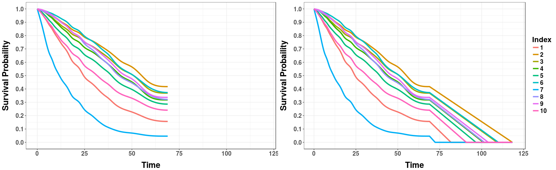
There are extreme cases where a survival model will predict a survival curve with survival probabilities of 1 (up to machine precision) for all survival times (think “a horizontal line, at ”) – this occurred for unregularized models on high-dimensional datasets. In these cases, this linear extrapolation will never reach 0. To address this, we fit the Kaplan-Meier curve with the linear extension described above to compute ; we then replace any infinite prediction with this value. Additionally, as the Kaplan-Meier curve is to represent the survival curve on a population level, we also truncated any patient’s median survival time by .
Appendix B Evaluation Measures Supplementary Information
This appendix provides additional information about the various evaluation measures.
B.1 Concordance
As discussed in Section 3.1, Concordance is designed to measure the discriminative ability of a model. This is challenging for censored data. For example, suppose we have two patients who were censored at and . Since both patients were censored, there is no way of knowing which patient died first and hence the risk scores for these patients are incomparable. However, if one patient’s censored time is later than the death time of another patient, we do know the true survival order of this pair: the second patient died before the first.
To be precise, we first need to define the set of comparable pairs, which is the subset of pairs of indices (here using the validation dataset () and recalling that indicates a patient who died (uncensored)) containing all pair of instances when we know which patient died first:
| (43) |
Notice when the earlier event is uncensored (a death), we know the ordering of the deaths (whether the second time is censored or not) – see Figure 14. The condition is to prevent double-counting such that .

We then consider how many of the possible pairs our predictor put in the correct order: That is, of all pairs in , we want to know how often given that . Hence, the Concordance index of , with respect to the risk scores, , is
| (44) |
One issue is how to handle ties, in either risk scores or death times – i.e., for two patients, Patient A and Patient B, consider either or . The two standard approaches are (1) to give the model a score of 0.5 for ties (of either risk scores or death times), or (2) to remove tied pairs entirely [54]. The first option is equivalent to Kendall’s tau, while the second leads to the Goodman-Kruskal gamma. The empirical evaluations (given in Section 4.2) use the first, as this gives Kaplan-Meier a Concordance index of 0.5 for all models. If we use the second option (excluding ties), then the Concordance for the Kaplan-Meier model is not well-defined.
B.2 L1-loss, and variants
As discussed in Section 3.2, survival analysis can be viewed as a regression problem that is attempting to minimize the difference between an estimated time of death and the true time of death. However, typical regression problems require having precise target values for each instance; here, many instances are censored – i.e., providing only lower bounds for the target values. One option is to simply remove all the censored patients and use the L1-loss given by Equation 4 (which we call “Uncensored L1-Loss”); however, this will likely bias the true loss. Table 11 in Appendix D.3 provides the results for this Uncensored L1-loss over the 8 datasets. (We see that mtlr is best for 6 of these datasets.)
One way to incorporate censoring is to use the Hinge loss for censored patients, which assigns loss to any patient whose censoring time is prior to the estimated median survival time, – i.e., a loss of 0 if – and a loss of if the censoring time is greater than . That is:
| (45) |
where is the subset of the validation dataset that is uncensored, and is the censored subset, and is the positive part of , i.e.,
This formulation is an optimistic lower bound on the L1-loss for two reasons: (1) it gives a loss of 0 if the censoring occurs prior to the estimated survival time, implying that , and (2) it gives a loss of if the censoring time occurs after the estimated survival time, which assumes that . Both are the best possible values for the unknown , given the constraints..
One weakness of the L1-Hinge loss is that if a model predicts very large survival times for all patients (both censored and observed), the hinge loss will give 0 loss for the censored patients; in datasets with a large proportion of censored patients, this leads to an optimistic score overall. Thus the hinge loss will favor models that tend to largely overestimate survival times as opposed to those models underestimating survival time.
A third variant of L1-loss, the L1-Margin loss, assigns a “Best-Guess” value to the death time corresponding to , which is the patient’s conditional expected survival time given they have survived up to – given by
| (48) |
where is the survival function; Theorem B.1 proves this value corresponds to the conditional expectation. In practice we use Kaplan-Meier estimate, , generated from the training dataset (disjoint from the validation dataset) as our estimate of in Equation 48.
We also realized that these estimates are more accurate for some patients, than for others. If – that is, if the patient was censored near the beginning time – then we know very little about the true timing of when the death occurred, so the estimate is quite vague, which suggests we should give very little weight to the associated loss, . Letting be the weight associated with these terms, we would like . On the other hand, if is large – towards the longest survival time observed (call it ) – then there is a relatively narrow gap of time where this could have died (probably within the small interval ); here, we should give a large weight to loss associated with this estimate.
This motivates us to define
| (49) |
where reflects the confidence in each Best-Guess estimate. To implement this, we set , which gives little weight to instances with early censor times but considers late censor times to be almost equivalent to an observed death time. Note this is the version of L1-loss we presented in Figure 11, with details in Table 10.
For completeness, we prove Equation 48. (This claim is also proven by Gupta and Bradley [20], which uses mean residual life rather than expected total life.)
Theorem B.1.
The conditional expectation of time of death, , given that a patient was censored at time , is given by: .
Proof.
Let be the r.v. for the time when a patient dies, and define
as the survival function – i.e., the probability that the patient dies after time . Given this, the conditional probability is
∎
Step B.2 is an application of Tonelli’s theorem [41], which lets us swap the order of integration for a non-negative function. As desired, this quantity, , is always at least . Moreover, when , this is
which is the expected value of the distribution for this survival curve (and exactly the claim of the Theorem).
B.2.1 Log L1-loss
The L1-loss measure implicitly assumes that the quality of a prediction, , depends only on how close it is to the truth – i.e., on . But this does not always match how we think of the error: if we predict Patient A will live for 120 months then found that he actually lived 117 months, we would consider our prediction very accurate. By contrast, if we predict Patient B will live 1 month, but then find she lived 4 months, we would consider this to be a poor prediction. Notice, however, the L1-loss for Patient A is 3 months, which is the same as the L1-loss for Patient B: 3 months!
This motivates us to consider the relative error, rather than an absolute error: here, as our prediction for Patient A is off by only 3 / 120 = 2.5%, we consider it good, whereas our prediction for Patient B is off by 3 / 1 = 300%. The Log-L1-loss reflects this:181818 Note that the times mentioned in “Doc, do I have a day, a week, a month or a year?” are basically in a log-scale.
| (53) |
To compute the average Log-L1-loss over the dataset , we can use Equation 4 but using rather than , etc. To avoid taking , we replace 0 with half the minimum, positive death time (see Section B.6). Table 12 in Appendix D.3 provides the results here, over the 8 datasets. (We see that mtlr is best for 4 of these datasets.)
B.3 1-Calibration
To demonstrate the description from Section 3.3, consider the following example: If there are patients, then 50/10 = 5 will be in each bin, and the first bin will contain the 5 with lowest predicted probability values, and the second bin will contain the next smallest 5 values, and so forth – e.g.,
Now consider the 5 patients who belong to . As the average of their probabilities is , we should expect 40% of these 5 individuals to die in the next 5 years – that is, 2 should die. We can then compare this prediction () with the actual number of these patients who died. We can similarly compare the number of patients who actually died to the number predicted (based on the average of these 5 probability values, which here is ), and so forth.
In general, we say that the predictor is 1-Calibrated if these predictions, for the bins, are sufficiently close to the actual number of deaths with respect to these bins. Here, we use the Hosmer–Lemeshow statistical test (given in Section 3.3) to see if the observed results were significant; repeating Equation 3.3:
where is the number of observed events, is the number of patients, is the average predicted probability, and subscript refers to within the th of bins.
B.3.1 Incorporating Censoring into 1-Calibration
Survival data typically contains some amount of censoring, making the exact number of deaths for the th bin, , unobservable when the bin contains patients censored before . That is, given a censored patient whose censoring time occurred before the time of interest () the patient may or may not have died by . There are many standard techniques for incorporating censoring [19]; we use the D’Agostino-Nam translation [12], which uses the within bin Kaplan-Meier curve in place of . Specifically, the test statistic is given by,
where is the height of the Kaplan-Meier curve generated by the patients in the th bin, evaluated at . We use as we are predicting the number of deaths and not which instead gives the probability of survival at . Note also that follows a distribution, as opposed to the distribution for Equation 3.3.
B.4 Brier Score Details
This section supplements the description of the Brier score given in Section 3.4, discussing (1) the decomposition of the Brier score into calibration and discrimination components, (2) the failure of the Integrated Brier score to incorporate the full distribution of probabilities in survival curves, and (3) how to incorporate censoring into the Brier score.
B.4.1 Brier Score Decomposition
As mentioned in Section 3.4, the Brier score can be separated into calibration and discriminatory components. The original separations were the the work of Sanders [42] and Murphy [36, 37] and later put into the context of calibration and discrimination (also known as refinement) by DeGroot and Fineberg [13].
Recall the notation and mathematical expression of the Brier score for a set of uncensored instances, ,
To simplify notation, let . The separation of the Brier score requires that a discrete, distinct number of predictions exist; here, assume there are distinct values for for .
Further, let be the total number of patients with as their prediction and hence . Finally, let be the observed proportion of patients who have died by and thus is the proportion still alive. The separation theorem of the Brier score states that , where and are nonnegative calibration and discriminatory scores where
| (54) | |||||
| (55) |
Note the calibration score, , is nearly equivalent (up to a factor of ) to the numerator of the Hosmer-Lemeshow test (Equation 3.3). However, the Hosmer-Lemeshow test subscript refers to bins whereas here the subscript refers to a distinct value of . One can see that represents a calibration score as the estimated probabilities, , must be close to the true proportion of deaths, in order to have a small score (lower is better). In fact, to satisfy , all predictions, must be equal to (Equation 54).
There are also similarities between and the denominator of the Hosmer-Lemeshow test. However, note Equation 55 uses the the true proportion of deaths , whereas the Hosmer-Lemeshow test uses an estimated value, . Note that has a “good” (low) score if all patients associated with a prediction probability have the same status – i.e., they either all die or are all still alive. To understand why this means is a discriminatory measure, consider the extreme case where , which means both and . For , all patients associated with each probability value must either be dead by or all be alive at – i.e., for ; note only is possible here. In turn, for , we require for , that is – all predictions will be 1 or 0. Here we are discriminating perfectly between the patients who have died and the patients who are still alive, with a model that predicts only 1’s or 0’s. Of course, we should not require a model to estimate survival probabilities to be precisely 1 or 0, for the same reason that we do not expect the learned distribution to correspond to the Heaviside distribution shown in Figure 5.
B.4.2 Integrated Brier score does not involve the Entire Distribution
At the beginning of Section 3.5, we claimed the Integrated Brier score (IBS) does not utilize the survival curves’ full distribution of probabilities over all times. For example, on a km curve, we expect that 10% of patients will die in every 10% interval – e.g., 10% of all patients will die in the [0.5, 0.6) interval. While D-Calibration will debit a model that fails to do this, this Integrated Brier score does not require this. The most obvious example is the perfect model, where each patient is given the appropriate Heaviside distribution (Figure 5) at his/her time-of-death: here the only probabilities are {0,1} – here IBS, even though no patient’s is ever in [0.5, 0.6). However, as we have previously noted, the inherent stochasticity of the world means that meaningful distributions should include non-zero probabilities in other places as well, rather than placing all weight on a single time point.
Since the Integrated Brier score fails to account for this, there is no guarantee that probabilities are meaningful across individual survival curves. This motivated us to introduce D-Calibration, to determine whether a proposed isd-model produces meaningful distributions, with probabilities that reflect the number of deaths that have occurred in the population. To see that these two metrics are measuring different aspects, note that the Integrated Brier scores for the (aft, cox-kp, coxen-kp, and mtlr) models are all well within 1 standard error of one another for the GBM dataset, but only coxen-kp and mtlr are D-Calibrated. (This is also true for the GLI dataset.)
B.4.3 Incorporating Censoring into the Brier score
In 1999, Graf et al. [18] proposed a way to compute the Brier Score for censored data, by using inverse probability of censoring weights (IPCW), which requires estimating the censoring survival function, denoted as over time points . We can estimate by the Kaplan-Meier curve of the censoring distribution – i.e., swapping those who are censored with those who are not, () and building the standard Kaplan-Meier model. Intuitively, this IPCW weighting counteracts the sparsity of later observations – if a patient dies early, there is a good chance that meaning the event is observed, but if the patient survives for a long time, it becomes more likely that meaning this patient will be censored. Gerds et al. [16, 17] formalizes and proves this intuition.
The censored version of the Brier score for a given time, , is calculated as
| (56) |
where . The first part of Equation 56 considers only uncensored patients whereas the second part counts all patients whose event time is greater than . The patients who were censored prior to are not explicitly included, but contribute based on their influence in .
As is a decreasing step function of , is increasing, which means that patients who survive longer than have larger weights than patients that died earlier, since the longer surviving patients were more likely to become censored.
B.5 D-Calibration
We begin this section by justifying why, in the case of all uncensored patients, (1) the distribution of the survival function, , should follow a uniform distribution, then (2) Following this discussion, we show how to incorporate censored patients into the D-Calibration estimate, and finally, (3) that this combination of censored and uncensored patients will produce a uniform distribution for the goodness-of-fit test to test against.
For this analysis, we assume each patient has a true survival function, , which is the probability that this patient will die after time . Assume each patient has a time of death, and a censoring time, , and is the observed event time. We also assume that censoring time is independent of death time, . Given a validation set , we first examine the case of all uncensored patients – i.e., for .
Lemma 1.
The distribution of a patient’s survival probability at the time of death is uniformly distributed on [0,1].
Proof.
The probability integral transform [4] states that, for any random continuous variable, , with cumulative distribution function given by , the random variable will follow a uniform distribution on [0,1], denoted as . Thus, given randomly sampled event times, , we have . As the survival function is simply , its distribution is , which also follows and hence . ∎
This Lemma shows that, given the true survival model, producing curves, the distribution of should be uniform over event times. Thus if a learned model accurately learns the true survival function, , we will expect the distribution across event times to be uniform. This is then tested using the goodness-of-fit test assuming each bin contains an equal proportions of patients.
Of course, conditions become more complicated when considering censored patients. Suppose we have a censored patient – i.e., – such that . Since the censoring time is a lower bound on the true death time, we know that , since and survival functions are monotonically decreasing as event time increases. If we are using deciles, we would like to know the probability that the time of death occurred in the [0.2,0.3) bin – i.e., . Using the rules of conditional probability, this is computationally straightforward191919To simplify notation, we drop the conditioning on of .:
| (as ) | ||||
Similarly, we can use the same logic as above to compute these probabilities for the other two bins, and :
| (as ) | ||||
and similarly for the bin. Note that these probabilities sum to one, , as desired.
This example motivates the following procedure to incorporate censored patients into the D-Calibration process: Given bins that equally divide [0,1] into intervals of width , suppose a patient is censored at time with associated survival probability . Let be the infimum probability of the bin that contains – e.g., 0.2 for the example above where . Then we assign the following weights to bins:
-
(A)
Bin (which contains ):
-
(B)
All following bins (i.e., the bins whose survival probabilities are all less than ): ,
Note this formulation follow directly from the example above. This weight assignment effectively “blurs” censored patients across the bins following the bin where the patient’s learned survival curve, placed the censored patient.
To further illustrate this concept of blurring a patient across bins, consider a patient who is censored at with . This patient is then blurred across all bins, adding a weight of 0.1 to all 10 bins. Alternatively, if a patient is censored very late, with then the patient is not blurred at all – only a weight of 1 is added to the last bin.
This identifies a weakness of D-Calibration: if a validation set contains patients censored at time 0, then all bins are given an equal weight of ; if is large relative to the total number of patients, then the bins may appear uniform, no matter how the other patients are distributed, which means any model based on such heavily “time 0 censored” data would be considered to be D-Calibrated.
To perform the goodness-of-fit test, we must first calculate the observed proportion of patients within each bin. Let represent the observed proportion of patients within the interval –e.g., in the example above. We can formally calculate:
| (57) | |||||
| (58) | |||||
| (59) |
Above, (57) refers to the weight that the patients with observed events contribute to the bin – i.e., each uncensored patient whose survival probability at time of death lands in contribute a value of . Here, we consider to be an uncensored event. Next, (58) gives the weight from the censored patients whose survival probability at time of censoring is within the bin (item (A) above). Lastly, (59) gives the weights from censored patients whose survival probability was contained in a previous bin (item (B) above).
Theorem B.2 below proves that the expected value of is equal for all bins – i.e., – which allows us to apply the goodness-of-fit test with uniform proportions.
We assume that all survival curves are strictly monotonically decreasing meaning we have the equality, ). This equivalence lets us replace with , within the indicator functions in . To simplify notation, we define , , and . The proof below shows that the expected value of the summand within Equations (57) – (59) above is equal to – i.e., we ignore and take the expected value of the term inside the summation.
Theorem B.2.
Proof.
| (I) | ||||
| (II) | ||||
| (III) |
Focusing on the second probability in line (I), note and imply that which can be expanded to the cases for and . Using this, we reformulate the probability by noting the equivalence of the event space,
Combining the second piece above with the first probability in line (I), we again simplify by noting these probabilities bound ,
Using this simplification we can rewrite the entirety of line (1),
Recalling the independence assumption, , we have the following equalities:
where the final equalities are due to the uniformity of the survival function on , . This then leaves the final simplification of line (I) as,
Now we address line (II) and analagously line (III):
| (Def. of ) | ||||
Here is the probability distribution function (PDF) for the distribution generated by the survival function applied to a censored observation. As the censoring distribution is unknown is also unknown whereas would be the PDF of the uniform distribution.
Following the steps above for line (III) analogously gives us
Combining the simplifications of lines (I), (II) and (III), we have the following,
| (I) | ||||
| (II) | ||||
| (III) | ||||
∎
This proof requires the assumption that survival curves are strictly monotonically decreasing on [0,1]. This means survival curves will not contain any large flat areas, which means there will not be non-zero probability mass for when , which means certain terms in the proof below would fail to cancel with one another, leaving us with non-equivalent proportions within each bin (specifically higher proportions within bins that contain these flat lines).
A natural corollary of Theorem B.2 is that all consistent estimators of the true survival distribution will be D-Calibrated (if the true survival distribution is strictly monotonic). Further, if survival time is independent and identically distributed (i.i.d.) across patients then there will only be one true survival curve for all patients, and thus, as Kaplan-Meier is uniformly consistent [5, 11]:
Lemma 2.
The Kaplan-Meier distribution is asymptotically D-Calibrated.
This is consistent with the results given in Section 4.2, which showed that km always passed the D-Calibration test with a -value 1.000, in all 8 datasets. Under all uncensored data, we would expect the typical 5% Type I error rate for claiming 0.05 as significant, however in the presence of censored data a correct estimate of the survival distribution the proportion within bins become smoothed, boosting the -value.
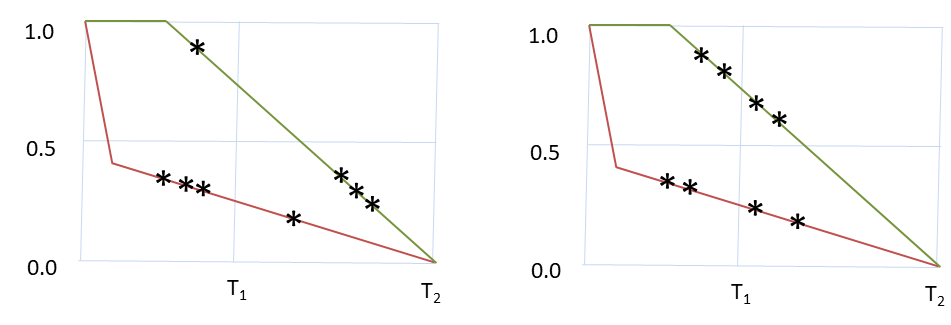
Proposition B.3.
It is possible for a isd model to be perfectly D-calibrated but not 1-calibrated at a time ; and for (another) isd model to be perfectly 1-calibrated at time but not D-calibrated.
Proof.
“1-Calibration D-Calibration”: Consider the model shown in Figure 15[left]. Here, the green curve corresponds to 4 apparently-identical patients , and the red curve, to apparently-identical . The “”s mark the time when each patient died, denoted as for . We intentionally use simple examples, with no censored patients, with curves that go to 0. Note this model assigns for each of the 4 green patients, and for each of the 4 red patients
To show that this model is 1-Calibrated, with respect to : Recall we first sort the values, then partition them into sets. Here, we consider , rather than the deciles earlier. The first set contains the 4 patients with (i.e., the green patients); and the second, the 4 patients with . Now note that 3 of the 4 “ patients” are alive at ; and 1 of the 4 “ patients” are alive at – which means this model is perfectly 1-Calibrated at .
However, this model is not D-Calibrated: To be consistent with the earlier 1-Calibration analysis, we partition the time intervals into 2 sets (not 10), as shown in Figure 15. Here, holds for only 1 patient, and holds for 7; if the model was D-Calibrated, each of these sets should contain 4 patients.
“D-Calibration 1-Calibration”: See Figure 15[right], where again, each line represent 4 different patients; notice the outcomes are different from those on the left. To see that this model is D-Calibrated, note there are 4 patients with (the green patients), and 4 with (for the red patients). However, the model is not 1-Calibrated, at : Of the 4 patients with , 2 are alive at ; and of the 4 patients with , 2 are alive at . To be 1-Calibrated, there should be 3 living patients in the first set, and 1 in the second; hence this model is not 1-Calibrated at . ∎
B.6 Other Subtle Points
All of these tools for producing survival curves are able to deal with “right censored” events: where the censored event time is a lower bound of the time of death. (This corresponds to, perhaps, the termination of a study, or when a participant left the study early.) There are other types of censoring, including “left censoring”, which provides an upper-bound on the time of death (e.g., when a survey finds that the patient is currently dead, but does not know when previously this happened), and “interval censoring”, when we can constrain the time of death to some interval. While there are extensions of each of these tools that can accommodate these alternate types of censoring, here we considered the most common case of having right-censored instances, and included only datasets that had only such instances.
As a second subtle issue: some of the methods involve taking the log of a predicted value, or of a true value; see Appendix B.2.1. This is clearly problematic if that value is 0 – e.g., if a patient died during a transplantation surgery. To avoid these errors, we replace any such 0 with the for a database, which is defined as 1/2 of the minimum observed positive time of any event, in that dataset. That is, we ignore all time=0 events, and then consider the smallest remaining value. If that value is, say, 1.0 day, then we set 0.5 days. Note that all other times are left unchanged.
Appendix C Comments about Various isd’s
C.1 Comments about cox-kp
Notice Equation 2 embodies two strong assumptions: (1) that the individual features are independent of one another (e.g., the outcome does not depend on a non-linear combination of the features), and (2) that these covariates are independent of time – which means that a blood test is as important just after an operation, as it is a year later, or a decade later. These assumptions mean the survival curves for different patients will have the same basic shape, and will not cross; see Figure 4 (middle-left). These simplifications allow the Cox model to suggest important information about individual features by examining the single coefficient associated with the feature, e.g., does “being male” increase the risk of dying from this specific cancer, or does it protect against this outcome (or neither). This “neither” case suggests that a given feature is not relevant to the prediction; for this reason, we used univariate Cox is a feature selection technique for our results.
By contrast, mtlr and rsf-km do not make these extreme assumptions, which means that a given feature can have different levels of importance at different times. Moreover, the curves for different patients can cross; see Figure 4. More relevant, however, we found that mtlr is more often D-Calibrated, and hence more meaningful for individual patients, than this “predictive Cox” system; see Table 6. While this Cox analysis of survival may not be directly relevant for individual patients, there are still extreme benefits in being able to identify important features. By observing how different features impact survival, clinicians can be made aware of treatments or lifestyle changes that best help patients survival.
C.2 Overview of mtlr
Consider202020 This paragraph is paraphrased from [57]; reprinted with permission of publisher/author. modeling the probability of survival of patients at each of a vector of time points – e.g., could be the 60 monthly intervals from 1 month up to 60 months. We can set up a series of logistic regression models: For each patient, represented as ,
| (60) |
where are the time-specific parameter vectors. While the input features stay the same for all these classification tasks, the binary labels can change depending on the threshold . We encode the survival time of a patient as a sequence of binary values: , where denotes the survival status of the patient at time , so that (no death event yet) for all with , and (death) for all with . Here there are possible legal sequences of the form212121 Notice there are no ‘0’s after a ‘1’. This is the ‘no zombie’ rule: once someone dies, that person stays dead. , including the sequence of all ‘0’s and the sequence of all ‘1’s. Our mtlr model computes the probability of observing the survival status sequence as:
where , and for is the score of the sequence with the event occurring in the interval before taking the logistic transform, with the boundary case being the score for the sequence of all ‘0’s. Given a dataset of patients with associated time of deaths , we find the optimal parameters (for the mtlr model) as
| (61) |
where the (for the regularizer) is found by an internal cross-validation process.
There are many details here – e.g., to insure that the survival function starts at 1.0, and decreases monotonically and smoothly until reaching 0.0 for the final time point; to deal appropriately with censored patients; to decide how many time points to consider (); and to minimize the risk of overfitting (by regularizing), and by selecting the relevant features. The paper by Yu et al. [57] provides the details.
Afterwards, the isd-Predictor can use the learned mtlr-model to produce a curve for a novel patient, who is represented as the vector of his/her covariates . This involves computing the values, ; the running sum of these values is essentially the survival curve. We then use splines to produce a smooth monotonically decreasing curve – such as the 10 such curves shown in Figure 4 (bottom-right).
C.3 Extension to Random Survival Forests (rsf-km)
Given a labeled dataset, a random survival forest learner will produce a set of decision trees from a bootstrapped sample of the training data. It grows each tree recursively, starting from the root – identifying each position with the set of patients who arrive there. For each position, the growth stops if there are fewer than deaths (where is chosen via cross-validation). Otherwise, it identifies the feature for this node: it first randomly draws a small random subset of the features to consider, then selects the feature (from that subset) that maximizes the difference in survival between two daughter nodes, based on the logrank test statistic (or some other chosen splitting rule). This becomes the rule of that node; and the learner then considers its two daughters, by splitting on the node’s feature.
Each leaf node in each tree corresponds to the set of training instances that reached that node. Given these learned trees, to classify a novel instance , the random forest performance system will drop into each of the trees, which will lead to different leaf nodes, then use the subsets of training instances to make a decision. Since each terminal node in the random survival forest contains a set of instances, we can use these instances to produce a Kaplan-Meier curve.222222 While the original paper does not consider survival curves, documentation https://kogalur.github.io/randomForestSRC/theory.html\#section8.1 describing the inner workings of the R package states that survival curves in terminal nodes are created via the Kaplan-Meier estimator.
Once the survival forest has been learned (with trees), a patient is dropped into each of the survival trees, leading to leaf nodes, which produces Kaplan-Meier curves. The rsf-km implementation then “averages” these curves, by taking a point-wise average across the curve for all time points – see Figure 16.232323 The method for generating individual survival curves could not be found in any of the literature by the authors of random survival forests. Survival curves were reverse-engineered by the authors of this paper – all survival curves tested matched the methodology explained here.
Note that the risk score generated by the median of the individual survival curves (produced here) does not necessarily result in the same ordering of patients as the risk scores of the original rsf implementation, which uses averaged cumulative hazards as a risk score. For this reason, we also applied the original rsf process to the datasets presented in the paper. We found that the Concordance scores were similar to that of rsf-km; mtlr still outperformed rsf on the datasets where mtlr outperformed rsf-km (data not shown).

Appendix D Detailed Empirical Results
This sub-appendix includes the tables that correspond to the figures given in Section 4.2. Further, Appendix D.4 provides the all -values for the 1-Calibration tests.
D.1 Concordance
| GBM | GLI | Nacd-Col | NACD | READ | BRCA | DBCD | DLBCL | ||
|---|---|---|---|---|---|---|---|---|---|
| km | 0.500 (0.000) | 0.500 (0.000) | 0.500 (0.000) | 0.500 (0.000) | 0.500 (0.000) | 0.500 (0.000) | 0.500 (0.000) | 0.500 (0.000)) | |
| aft | 0.692 (0.026) | 0.802 (0.011) | 0.722 (0.015) | 0.755 (0.008) | 0.700 (0.183) | 0.738 (0.041) | 0.474 (0.056) | 0.558 (0.046) | |
| cox-kp | 0.696 (0.026) | 0.805 (0.01) | 0.722 (0.015) | 0.755 (0.008) | 0.716 (0.157) | 0.747 (0.030) | - | - | |
| coxen-kp | 0.698 (0.032) | 0.801 (0.006) | 0.726 (0.024) | 0.754 (0.009) | 0.731 (0.141) | 0.761 (0.032) | 0.744 (0.055) | 0.695 (0.038) | |
| rsf-km | 0.650 (0.038) | 0.776 (0.021) | 0.743 (0.024) | 0.758 (0.005) | 0.582 (0.093) | 0.704 (0.036) | 0.738 (0.060) | 0.639 (0.038) | |
| mtlr | 0.703 (0.032) | 0.812 (0.013) | 0.734 (0.023) | 0.757 (0.008) | 0.768 (0.091) | 0.770 (0.027) | 0.766 (0.065) | 0.704 (0.034) |
D.2 Brier Score
| GBM | GLI | Nacd-Col | NACD | READ | BRCA | DBCD | DLBCL | ||
|---|---|---|---|---|---|---|---|---|---|
| km | 0.046 (0.001) | 0.034 (0.000) | 0.083 (0.001) | 0.089 (0.000) | 0.027 (0.005) | 0.017 (0.001) | 0.097 (0.003) | 0.109 (0.004) | |
| aft | 0.041 (0.003) | 0.021 (0.002) | 0.066 (0.003) | 0.065 (0.002) | 0.026 (0.017) | 0.0133 (0.002) | 0.254 (0.023) | 0.295 (0.038) | |
| cox-kp | 0.040 (0.003) | 0.022 (0.003) | 0.066 (0.003) | 0.067 (0.002) | 0.026 (0.017) | 0.014 (0.002) | - | - | |
| coxen-kp | 0.040 (0.003) | 0.021 (0.002) | 0.064 (0.003) | 0.065 (0.001) | 0.024 (0.011) | 0.015 (0.002) | 0.070 (0.004) | 0.078 (0.013) | |
| rsf-km | 0.059 (0.009) | 0.051 (0.009) | 0.079 (0.006) | 0.079 (0.001) | 0.047 (0.013) | 0.028 (0.002) | 0.077 (0.003) | 0.095 (0.013) | |
| mtlr | 0.039 (0.004) | 0.019 (0.002) | 0.062 (0.003) | 0.063 (0.001) | 0.023 (0.006) | 0.012 (0.001) | 0.070 (0.003) | 0.078 (0.011) |
D.3 Empirical Values of L1-Loss, and Variants
Here we give the the results for the Margin-L1-loss (Table 10) as given in Figure 11. Additionally, we give results for the Uncensored L1-loss (Table 11) and the Log-Margin-L1-loss (Table 12).
| GBM | GLI | Nacd-Col | NACD | READ | BRCA | DBCD | DLBCL | ||
|---|---|---|---|---|---|---|---|---|---|
| km | 1431.31 (59.25) | 2746.70 (91.85) | 56.45 (1.95) | 61.97 (0.50) | 3677.90 (222.77) | 5392.04 (128.19) | 24.88 (0.78) | 20.28 (2.06) | |
| aft | 1240.60 (57.38) | 1838.20 (105.23) | 47.89 (1.85) | 43.99 (1.44) | 4068.72 (1451.14) | 5156.1 (264.50) | 47.01 (4.38) | 27.29 (3.31) | |
| cox-kp | 1278.18 (44.02) | 1824.06 (127.49) | 45.53 (2.23) | 44.26 (1.29) | 4799.91 (1460.52) | 6247.01 (612.3) | - | - | |
| coxen-kp | 1347.36 (51.6) | 1683.04 (110.82) | 45.25 (1.94) | 45.72 (1.43) | 3564.01 (1163.92) | 4593.52 (370.75) | 24.28 (2.14) | 15.97 (1.10) | |
| rsf-km | 1399.17 (99.06) | 4503.49 (465.47) | 58.81 (2.28) | 49.69 (1.38) | 6805.00 (1710.50) | 10934.45 (579.44) | 26.58 (2.35) | 17.68 (1.81) | |
| mtlr | 1271.73 (37.71) | 1582.72 (131.1) | 43.48 (2.52) | 43.97 (1.20) | 3417.49 (256.83) | 4669.55 (153.50) | 20.01 (1.47) | 15.52 (1.97) |
| GBM | GLI | Nacd-Col | NACD | READ | BRCA | DBCD | DLBCL | ||
|---|---|---|---|---|---|---|---|---|---|
| km | 318.53 (10.49) | 520.32 (9.56) | 19.40 (0.15) | 12.17 (0.08) | 1829.99 (1261.87) | 2418.79 (24.55) | 18.69 (0.64) | 2.90 (0.20) | |
| aft | 291.28 (28.99) | 524.78 (64.89) | 19.58 (1.38) | 12.54 (1.07) | 1738.27 (1191.64) | 2681.47 (453.66) | 23.77 (3.95) | 13.48 (3.01) | |
| cox-kp | 281.61 (26.53) | 542.35 (76.2) | 18.91 (1.35) | 12.63 (1.12) | 2248.56 (1263.39) | 3141.20 (521.90) | - | - | |
| coxen-kp | 284.86 (14.93) | 482.70 (44.76) | 16.14 (1.12) | 10.64 (0.66) | 1936.34 (1186.59) | 2647.76 (399.62) | 11.52 (1.51) | 3.19 (1.38) | |
| rsf-km | 373.14 (72.48) | 1204.95 (276.78) | 28.33 (2.15) | 15.61 (1.07) | 4099.14 (1482.32) | 5671.22 (511.99) | 13.07 (1.51) | 3.91 (0.93) | |
| mtlr | 272.20 (27.15) | 436.99 (62.40) | 15.87 (1.03) | 10.71 (0.57) | 1411.46 (306.97) | 2167.09 (208.32) | 9.30 (1.30) | 3.70 (0.92) |
| GBM | GLI | Nacd-Col | NACD | READ | BRCA | DBCD | DLBCL | ||
|---|---|---|---|---|---|---|---|---|---|
| km | 1.98 (0.01) | 2.35 (0.02) | 1.76 (0.04) | 2.20 (0.01) | 2.05 (0.19) | 1.78 (0.03) | 2.02 (0.04) | 3.37 (0.11) | |
| aft | 1.64 (0.08) | 1.36 (0.06) | 1.44 (0.01) | 1.48 (0.04) | 2.00 (0.60) | 1.65 (0.14) | 6.21 (0.68) | 10.54 (2.62) | |
| cox-kp | 1.68 (0.07) | 1.35 (0.06) | 1.42 (0.02) | 1.48 (0.04) | 2.02 (0.56) | 1.73 (0.11) | - | - | |
| coxen-kp | 1.80 (0.01) | 1.35 (0.05) | 1.43 (0.03) | 1.55 (0.05) | 1.88 (0.56) | 1.56 (0.06) | 1.77 (0.08) | 2.70 (0.11) | |
| rsf-km | 1.85 (0.20) | 1.98 (0.10) | 1.51 (0.05) | 1.54 (0.04) | 2.62 (0.47) | 2.21 (0.12) | 1.90 (0.05) | 3.04 (0.14) | |
| mtlr | 1.67 (0.07) | 1.25 (0.08) | 1.37 (0.05) | 1.50 (0.04) | 1.95 (0.17) | 1.57 (0.06) | 1.67 (0.07) | 2.60 (0.18) |
D.4 1-Calibration
Each table corresponds to a different percentile of event times for each dataset. Moving down the 10th, 25th, 50th, 75th, and 90th percentiles are given. Bolded values indicate models which passed 1-Calibration (). The “Total” column of each table gives the total number of datasets passed by each model – that is, the values in that columns correspond to Table 5.
| GBM | GLI | Nacd-Col | NACD | READ | BRCA | DBCD | DLBCL | Total | ||
|---|---|---|---|---|---|---|---|---|---|---|
| aft | 0.001 | 0.159 | 0.794 | 0.012 | 1.000 | 0.919 | 0.000 | 0.000 | 4 | |
| cox-kp | 0.001 | 0.140 | 0.794 | 0.008 | 0.999 | 0.782 | - | - | 4 | |
| coxen-kp | 0.000 | 0.033 | 0.043 | 0.000 | 0.999 | 0.561 | 0.454 | 0.646 | 4 | |
| rsf-km | 0.000 | 0.000 | 0.078 | 0.016 | 0.998 | 0.000 | 0.164 | 0.273 | 4 | |
| mtlr | 0.908 | 0.450 | 0.440 | 0.047 | 1.000 | 0.929 | 0.000 | 0.177 | 6 |
| GBM | GLI | Nacd-Col | NACD | READ | BRCA | DBCD | DLBCL | Total | ||
|---|---|---|---|---|---|---|---|---|---|---|
| aft | 0.000 | 0.040 | 0.586 | 0.009 | 0.000 | 0.205 | 0.000 | 0.000 | 2 | |
| cox-kp | 0.000 | 0.008 | 0.379 | 0.003 | 0.000 | 0.535 | - | - | 2 | |
| coxen-kp | 0.000 | 0.002 | 0.003 | 0.000 | 0.238 | 0.044 | 0.436 | 0.547 | 3 | |
| rsf-km | 0.000 | 0.000 | 0.312 | 0.006 | 0.000 | 0.000 | 0.042 | 0.227 | 2 | |
| mtlr | 0.963 | 0.312 | 0.645 | 0.254 | 0.449 | 0.448 | 0.177 | 0.052 | 8 |
| GBM | GLI | Nacd-Col | NACD | READ | BRCA | DBCD | DLBCL | Total | ||
|---|---|---|---|---|---|---|---|---|---|---|
| aft | 0.117 | 0.030 | 0.035 | 0.043 | 0.000 | 0.000 | 0.000 | 0.000 | 1 | |
| cox-kp | 0.495 | 0.005 | 0.038 | 0.124 | 0.000 | 0.017 | - | - | 2 | |
| coxen-kp | 0.019 | 0.000 | 0.000 | 0.000 | 0.049 | 0.000 | 0.025 | 0.822 | 1 | |
| rsf-km | 0.000 | 0.000 | 0.761 | 0.001 | 0.000 | 0.000 | 0.000 | 0.068 | 2 | |
| mtlr | 0.796 | 0.306 | 0.813 | 0.112 | 0.995 | 0.013 | 0.041 | 0.262 | 6 |
| GBM | GLI | Nacd-Col | NACD | READ | BRCA | DBCD | DLBCL | Total | ||
|---|---|---|---|---|---|---|---|---|---|---|
| aft | 0.378 | 0.000 | 0.002 | 0.002 | 0.000 | 0.000 | 0.000 | 0.000 | 1 | |
| cox-kp | 0.008 | 0.000 | 0.003 | 0.004 | 0.087 | 0.016 | - | - | 1 | |
| coxen-kp | 0.338 | 0.000 | 0.000 | 0.000 | 0.001 | 0.000 | 0.003 | 0.436 | 2 | |
| rsf-km | 0.000 | 0.000 | 0.070 | 0.003 | 0.000 | 0.000 | 0.002 | 0.038 | 1 | |
| mtlr | 0.140 | 0.565 | 0.044 | 0.045 | 0.026 | 0.000 | 0.036 | 0.218 | 3 |
| GBM | GLI | Nacd-Col | NACD | READ | BRCA | DBCD | DLBCL | Total | ||
|---|---|---|---|---|---|---|---|---|---|---|
| aft | 0.000 | 0.000 | 0.000 | 0.000 | 0.000 | 0.000 | 0.000 | 0.000 | 0 | |
| cox-kp | 0.000 | 0.000 | 0.000 | 0.000 | 0.000 | 0.000 | - | - | 0 | |
| coxen-kp | 0.050 | 0.000 | 0.004 | 0.000 | 0.000 | 0.000 | 0.010 | 0.112 | 2 | |
| rsf-km | 0.000 | 0.000 | 0.000 | 0.000 | 0.000 | 0.000 | 0.000 | 0.023 | 0 | |
| mtlr | 0.109 | 0.148 | 0.000 | 0.001 | 0.000 | 0.000 | 0.098 | 0.157 | 4 |