Understanding and Improving Kernel Local Descriptors

Abstract

We propose a multiple-kernel local-patch descriptor based on efficient match kernels from pixel gradients. It combines two parametrizations of gradient position and direction, each parametrization provides robustness to a different type of patch mis-registration: polar parametrization for noise in the patch dominant orientation detection, Cartesian for imprecise location of the feature point. Combined with whitening of the descriptor space, that is learned with or without supervision, the performance is significantly improved. We analyze the effect of the whitening on patch similarity and demonstrate its semantic meaning. Our unsupervised variant is the best performing descriptor constructed without the need of labeled data. Despite the simplicity of the proposed descriptor, it competes well with deep learning approaches on a number of different tasks.

1 Introduction

Representing and matching local features is an essential step of several computer vision tasks. It has attracted a lot of attention in the last decades, when local features still were a required step of most approaches. Despite the large focus on Convolutional Neural Networks (CNN) to process whole images, local features still remain important and necessary for tasks such as Structure-from-Motion (SfM) FGGJR10 ; HSD+15 ; SF16 , stereo matching MMPL15 , or retrieval under severe change in viewpoint or scale SRCF15 ; ZZS+17 .

Classical approaches involve hand-crafted design of a local descriptor, which has been the practice for more than a decade with some widely used examples L04 ; BETV09 ; MS05 ; TLF10 ; CLSF10 ; LCS11 . Such descriptors do not require any training data or supervision. This kind of approach allows to easily inject domain expertise, prior knowledge or even the result of a thorough analysis DS15 . Learning methods have been also employed in order to learn parts of the hand-crafted design, e.g. the pooling regions WB07 ; SVZ13 , from the training data.

Recently, the focus has shifted from hand-crafted descriptors to CNN-based descriptors. Learning such descriptors relies on large training sets of patches, that are commonly provided as a side-product of SfM WB07 . Integrating domain expertise has been mostly so far neglected in this kind of approaches. Nevertheless, remarkable performance is achieved on a standard benchmark BRPM16 ; TW17 ; MMR+17 . On the other hand, recent work BLVM17 ; SLJS17 shows that many CNN-based approaches do not necessarily generalize equally well on different tasks or different datasets. Hand-crafted descriptors still appear an attractive alternative.

In this work, we choose to work with a particular family of hand-crafted descriptors, the so called kernel descriptors BS09 ; BRF11 ; TBFJ15 . They provide a quite flexible framework for matching sets, patches in our case, by encoding different properties of the set elements, pixels in our case. In particular, we build upon the hand-crafted kernel descriptor proposed by Bursuc et al. BTJ15 that is shown to have good performance, even compared to learned alternatives. Its few parameters are easily tuned on a validation set, while it is shown to perform well on multiple tasks, as we confirm in our experiments.

Further post-processing or descriptor normalization, such as Principal Component Analysis (PCA) and power-law normalization, is shown to be effective on different tasks DGJP13 ; BTJ15 ; MM07 ; TTO16 . We combine our descriptor with such post-processing that is learned from the data in unsupervised or supervised ways. We show how to reduce the estimation error and significantly improve results even without any supervision.

The hand-crafted nature and simplicity of our descriptor allows to visualize and analyze its parametrization, and finally understand its advantages and disadvantages. It leads us to propose a simple combination of parametrizations each offering robustness to different types of patch miss-registrations. Interestingly, the same analysis is possible even for the learned post-processing. We observe that its effect on the patch similarity is semantically meaningful. The feasibility of such analysis and visualization is an advantage or our approach, and hand-crafted approaches in general, compared to CNN-based methods. Several insightful ablation and visualization studies ZF14 ; YCN+15 ; MV16 ; BZK+17 reveal what a CNN has learned. This typically provides only a partial view, i.e. for a small number of neurons, on their behavior, while our approach enables visualization of the overall learned similarity in a general way that is not restricted to particular examples.

This work is an extension of our earlier conference publication MTC17 . In addition to the earlier version, we propose unsupervised whitening with shrinkage, give extra insight about its effect on patch similarity, present extended comparisons of different whitening variants and provide a proof justifying the absence of regularized concatenation.

The manuscript is organized as follows. Related work is discussed in Section 2, and background knowledge for kernel descriptors is presented in Section 3. Our descriptor, the different whitening variants, and their interpretation are described in Section 4. Finally, the experimental validation on two patch benchmarks is presented in Section 5.

2 Related work

We review prior work on local descriptors, covering both hand-crafted and learned ones.

2.1 Hand-crafted descriptors

Hand-crafted descriptors have dominated the research landscape and a variety of approaches and methodologies exists. There are different variants on descriptors building features from filter-bank responses BETV09 ; BSW05 ; KY08 ; OT01 ; SMo97 , pixel gradients L04 ; MS05 ; TLF10 ; AY11 , pixel intensities SI07 ; CLSF10 ; LCS11 ; RRKB11 , ordering or ranking of pixel intensities OPM02 ; HPS09 , local edge shape FL07 . Some approaches focus on particular aspects of the local descriptors, such as a injecting invariance in the patch descriptor OPM02 ; LSP05 ; AMHP09 ; TTO16 , computational efficiency TLF10 ; AY11 , binary descriptors CLSF10 ; LCS11 ; AOV12 .

A popular direction is that of gradient histogram-based descriptors, where the most popular representative is SIFT L04 . SIFT is a long-standing top performer on multiple benchmarks and tasks across the years. Multiple improvements for SIFT have been subsequently proposed: PCA-SIFT KeS04 , ASIFT YM09 , OpponentSIFT SGS10 , 3D-SIFT SAS07 , RootSIFT AZ12 , DSP-SIFT DS15 , etc. A simple and effective improvement of SIFT is brought by the RootSIFT descriptor AZ12 , which uses Hellinger kernel as similarity measure. DSP-SIFT DS15 counters the aliasing effects caused by the binned quantization in SIFT by pooling gradients over multiple scales instead of only the scale selected by SIFT. Our kernelized descriptor also deals with quantization artifacts by embedding each pixel in a continuous space and the aggregating pixels per patch by sum-pooling.

Kernel descriptors based on the idea of Efficient Match Kernels (EMK) BS09 encode entities inside a patch (such a gradient, color, etc.) in a continuous domain, rather than as a histogram. The kernels and their few parameters are often hand-picked and tuned on a validation set. Kernel descriptors are commonly represented by a finite-dimensional explicit feature maps VZ12 . Quantized descriptors, such as SIFT, can be also interpreted as kernel descriptor BTJ15 ; BRF10 . Furthermore, the widely used RootSIFT descriptor AZ12 can be also thought of as an explicit feature map from the original SIFT space to the RootSIFT space, such that the Hellinger kernel is linearised, i.e. the linear kernel (i.e. dot product) in RootSIFT space is equivalent to the Hellinger kernel in the original SIFT space. In this case, the feature mapping is performed by $\ell_{1}$-normalization and square-rooting, without any expansion in dimensionality.

In this work we build upon EMK by integrating multiple pixel attributes in the patch descriptor. Unlike EMK which relies on features from random projections that require subsequent learning, we leverage instead explicit feature maps to approximate a kernel behavior directly. These representations can be further improved by minimal learning.

2.2 Learned descriptors

Learned descriptors commonly require annotation at patch level. Therefore, research in this direction is facilitated by the release of datasets that originate from an SfM system WB07 ; PDHM+15 . Such training datasets allow effective learning of local descriptors, and in particular, their pooling regions WB07 ; SVZ13 , filter banks WB07 , transformations for dimensionality reduction SVZ13 or embeddings PISZ10 .

Kernelized descriptors are formulated within a supervised framework by Wang et al. WWZX+13 , where image labels enable kernel learning and dimensionality reduction. In this work, we rather focus on learning discriminative projections with minimal or no supervision. This is several orders of magnitude faster to learn than other learning approaches.

Recently, local descriptor learning is dominated by deep learning. The proposed network architectures mimic the ones for full-image processing. They have fewer parameters, however they still use a large amount of training patches.

Among representative examples is the work of Simo-Serra et al. STFK+15 training with hard positive and negative examples or the work of Zagoruyko ZK15 where a central-surround representation is found to be immensely beneficial. Such CNN-based approaches are seen as joint feature, filter bank, and metric learning HLJS+15 since both the convolutional filters, patch descriptor and metrics are learned end-to-end. Going further towards an end-to-end pipeline for patch detection and description, LIFT YTL+16 advances a multi-step architecture with several spatial transformer modules JSZ15 that detects interest points and crops them, identifies their dominant orientation and rotates them accordingly and finally extract a patch descriptor. Paulin et al. PMD+16 propose a deep patch descriptor from unsupervised learning. They consider a convolutional kernel network MKHS14 with feature maps compatible with the Gaussian kernel and which require layer-wise training.

Recent works in deep patch descriptors lean towards more compact architectures with more carefully designed training strategies and loss functions. Balntas et al. BRPM16 ; BJTM16 advance shallower architectures with improved triplet ranking loss BRPM16 ; BJTM16 . In L2-Net TW17 supervision is imposed on intermediate feature maps, the loss function integrates multiple attributes, while sampling of training data is done progressively to better balance positive and negative pairs at each step. In HardNet MMR+17 , Mishchuk et al. extend L2-Net with a loss that mimics Lowe’s matching criterion by maximizing the distance between the closest positive and closest negative example in the batch. HardNet is currently a top perfomer on most benchmarks. Despite obtaining impressive results on standard benchmarks, the generalization of CNN-based local descriptors to other datasets is not always the case SLJS17 .

2.3 Post-processing

A post-processing step is common to both hand-crafted and learned descriptors. This post-processing ranges from simple $\ell_{2}$ normalization, PCA dimensionality reduction, to transformations learned on annotated data RTC16 ; BHW11 ; BLVM17 ; JC12 .

3 Preliminaries

3.1 Kernelized descriptors.

In general lines we follow the formulation of Bursuc et al. BTJ15 . We represent a patch $\mathcal{P}$ as a set of pixels $p\in\mathcal{P}$ and compare two patches $\mathcal{P}$ and $\mathcal{Q}$ via a match kernel

$$\mathcal{M}(\mathcal{P},\mathcal{Q})=\sum_{p\in\mathcal{P}}\sum_{q\in\mathcal{Q}}k(p,q),$$ (1)

where kernel $k:\mathbb{R}^{n}\times\mathbb{R}^{n}\rightarrow\mathbb{R}$ is a similarity function, typically non-linear, comparing two pixels or their corresponding feature vectors. The evaluation of this match kernel is costly as it computes exhaustively similarities between all pairs of pixels from the two sets. Match kernel $\mathcal{M}(\mathcal{P},\mathcal{Q})$ can be approximated with EMK BS09 . It uses an explicit feature map $\psi:\mathbb{R}^{n}\rightarrow\mathbb{R}^{d}$ to approximate this result as

$$\begin{split}\mathcal{M}(\mathcal{P},\mathcal{Q})&=\sum_{p\in\mathcal{P}}\sum_{q\in\mathcal{Q}}k(p,q)\\ &\approx\sum_{p\in\mathcal{P}}\sum_{q\in\mathcal{Q}}\psi(p)^{\top}\psi(q)\\ &=\sum_{p\in\mathcal{P}}\psi(p)^{\top}\sum_{q\in\mathcal{Q}}\psi(q).\end{split}$$ (2)

Vector $\mathbf{V}(\mathcal{P})=\sum_{p\in\mathcal{P}}\psi(p)$ is a kernelized descriptor (KD), associated with patch $\mathcal{P}$, used to approximate $\mathcal{M}(\mathcal{P},\mathcal{Q})$, whose explicit evaluation is costly. The approximation is given by a dot product $\mathbf{V}(\mathcal{P})^{\top}\mathbf{V}(\mathcal{Q})$, where $\mathbf{V}(\mathcal{P})\in\mathbb{R}^{d}$. To ensure a unit self similarity, $\ell_{2}$-normalization by a factor $\gamma$ is introduced. The normalized KD is then given by $\bar{\mathbf{V}}(\mathcal{P})=\gamma(\mathcal{P})\mathbf{V}(\mathcal{P})$, where $\gamma(\mathcal{P})=(\mathbf{V}(\mathcal{P})^{\top}\mathbf{V}(\mathcal{P}))^{-\nicefrac{{1}}{{2}}}$.

Kernel $k$ comprises products of kernels, each kernel acting on a different scalar pixel attribute

$$k(p,q)=k_{1}(p_{1},q_{1})k_{2}(p_{2},q_{2})\ldots k_{n}(p_{n},q_{n}),$$ (3)

where kernel $k_{n}$ is pairwise similarity function for scalars and $p_{n}$ are pixel attributes such as position and gradient orientation. Feature map $\psi_{n}$ corresponds to kernel $k_{n}$ and feature map $\psi$ is constructed via Kronecker product of individual feature maps $\psi(p)=\psi_{1}(p_{1})\otimes\psi_{2}(p_{2})\otimes\ldots\otimes\psi_{n}(p_{n})$. It is straightforward to show that

$$\psi(p)^{\top}\psi(q)\approx k_{1}(p_{1},q_{1})k_{2}(p_{2},q_{2})\ldots k_{n}(p_{n},q_{n}).$$ (4)

3.2 Feature maps.

As non-linear kernel for scalars we use the normalized Von Mises probability density function, which is used for image TBFJ15 and patch BTJ15 representations. It is parametrized by $\kappa$ controlling the shape of the kernel, where lower $\kappa$ corresponds to wider kernel, i.e. less selective kernel. We use a stationary (shift invariant) kernel that, by definition, depends only on the difference $\Delta_{n}=p_{n}-q_{n}$, i.e. $k_{\mathsf{VM}}(p_{n},q_{n}):=k_{\mathsf{VM}}(\Delta_{n})$. We approximate this probability density function with Fourier series with $N$ frequencies that produces a feature map $\psi_{\mathsf{VM}}:\mathbb{R}\rightarrow\mathbb{R}^{2N+1}$. It has the property that

$$k_{\mathsf{VM}}(p_{n},q_{n})\approx\psi_{\mathsf{VM}}(p_{n})^{\top}\psi_{\mathsf{VM}}(q_{n}).$$ (5)

In particular we approximate the Fourier series by the sum of the first $N$ terms as

$$k_{\mathsf{VM}}(\Delta_{n})\approx\sum_{i=0}^{N}\gamma_{i}\cos(i\Delta_{n}).$$ (6)

The feature map $\psi_{\mathsf{VM}}(p_{n})$ is designed as follows:

$$\small\psi_{\mathsf{VM}}(p_{n})=(\sqrt{\gamma_{0}},\sqrt{\gamma_{1}}\cos(p_{n}),\ldots,\sqrt{\gamma_{N}}\cos(Np_{n}),\\ \sqrt{\gamma_{1}}\sin(p_{n}),\ldots,\sqrt{\gamma_{N}}\sin(Np_{n}))^{\top}.$$ (7)

This vector has $2N+1$ components. It is now easy to show that the inner product of two feature maps is approximating the kernel . That is,

$$\psi_{\mathsf{VM}}(p_{n})^{\top}\psi_{\mathsf{VM}}(q_{n}) =\gamma_{0}+\sum_{i=1}^{N}\gamma_{i}(\cos(ip_{n})\cos(iq_{n})$$ (8)

$$~{}~{}~{}~{}~{}~{}~{}~{}~{}~{}~{}~{}~{}~{}~{}~{}+\sin(ip_{n})\sin(iq_{n}))$$

$$=\sum_{i=0}^{N}\gamma_{i}\cos(i(p_{n}-q_{n}))$$

$$\approx k_{\mathsf{VM}}(\Delta_{n}).$$

The reader is encouraged to read prior work for details on these feature maps VZ10 ; Chum15 , which are previously used in various contexts TBFJ15 ; BTJ15 .

3.3 Descriptor post-processing.

It is known that further descriptor post-processing RTC16 ; BL15 ; BTJ15 is beneficial. In particular, KD is further centered and projected as

$$\hat{\mathbf{V}}(\mathcal{P})=A^{\top}(\bar{\mathbf{V}}(\mathcal{P})-\mu),$$ (9)

where $\mu\in\mathbb{R}^{d}$ and $A\in\mathbb{R}^{d\times d}$ are the mean vector and the projection matrix. These are commonly learned by PCA JC12 or with supervision RTC16 . The final descriptor is always $\ell_{2}$-normalized in the end.

4 Method

In this section we consider different patch parametrizations and kernels that result in different patch similarity. We discuss the benefits of each and propose how to combine them. We further learn descriptor transformation with or without supervision and provide useful insight on how patch similarity is affected.

4.1 Patch attributes.

We consider a pixel $p$ to be associated with coordinates $p_{x}$, $p_{y}$ in Cartesian coordinate system, coordinates $p_{\rho}$, $p_{\phi}$ in polar coordinate system, pixel gradient magnitude $p_{m}$, and pixel gradient angle $p_{\theta}$. Angles $p_{\theta}$, $p_{\phi}$ $\in[0,2\pi]$, distance from the center $p_{\rho}$ is normalized to $[0,1]$, while coordinates $p_{x}$, $p_{y}$ $\in\{1,2,\ldots,W\}$ for $W\times W$ patches. In order to use feature map $\psi_{\mathsf{VM}}$, attributes $p_{\rho}$, $p_{x}$, and $p_{y}$ are linearly mapped to $[0,\pi]$. The gradient angle is expressed w.r.t. the patch orientation, i.e. $p_{\theta}$ directly, or w.r.t. to the position of the pixel. The latter is given as $p_{\tilde{\theta}}=p_{\theta}-p_{\phi}$.

Figure 1: Kernel approximations that we use for pixel attributes. Parameter $\kappa$ and the number of frequencies $N$ define the final shape. The choice of kernel parameters is guided by BTJ15 .

4.2 Patch parametrizations.

Composing patch kernel $k$ as a product of kernels over different attributes enables easy design of various patch similarities. Correspondingly, this defines different KD. All attributes $p_{x}$, $p_{y}$, $p_{\rho}$, $p_{\theta}$, $p_{\phi}$, and $p_{\tilde{\theta}}$ are matched by the Von Mises kernel, namely, $k_{x}$, $k_{y}$, $k_{\rho}$, $k_{\theta}$, $k_{\phi}$, and $k_{\tilde{\theta}}$ parameterized by $\kappa_{x}$, $\kappa_{y}$, $\kappa_{\rho}$, $\kappa_{\theta}$, $\kappa_{\phi}$, and $\kappa_{\tilde{\theta}}$, respectively. In a similar manner to SIFT, we apply a Gaussian mask by $p_{g}=\exp(-p_{\rho}^{2})$ which gives more importance to central pixels.

In this work we focus on the two following match kernels over patches. One in polar coordinates

$$\mathcal{M}_{\phi\rho\tilde{\theta}}(\mathcal{P},\mathcal{Q})=\sum_{p\in\mathcal{P}}\sum_{q\in\mathcal{Q}}p_{g}q_{g}\sqrt{p_{m}}\sqrt{q_{m}}k_{\phi}(p_{\phi},q_{\phi})\\ k_{\rho}(p_{\rho},q_{\rho})k_{\tilde{\theta}}(p_{\tilde{\theta}},q_{\tilde{\theta}}),$$ (10)

and one in Cartesian coordinates

$$\mathcal{M}_{xy\theta}(\mathcal{P},\mathcal{Q})=\sum_{p\in\mathcal{P}}\sum_{q\in\mathcal{Q}}p_{g}q_{g}\sqrt{p_{m}}\sqrt{q_{m}}k_{x}(p_{x},q_{x})\\ k_{y}(p_{y},q_{y})k_{\theta}(p_{\theta},q_{\theta}).$$ (11)

The KD for the two cases are given by

$$\mathbf{V}_{\phi\rho\tilde{\theta}}(\mathcal{P}) =\sum_{p\in\mathcal{P}}p_{g}\sqrt{p_{m}}\psi_{\phi}(p_{\phi})\otimes\psi_{\rho}(p_{\rho})\otimes\psi_{\tilde{\theta}}(p_{\tilde{\theta}})$$ (12)

$$=\sum_{p\in\mathcal{P}}p_{g}\sqrt{p_{m}}\psi_{\phi\rho\tilde{\theta}}(p)$$

$$\mathbf{V}_{xy\theta}(\mathcal{P}) =\sum_{p\in\mathcal{P}}p_{g}\sqrt{p_{m}}\psi_{x}(p_{x})\otimes\psi_{y}(p_{y})\otimes\psi_{\theta}(p_{\theta})$$ (13)

$$=\sum_{p\in\mathcal{P}}p_{g}\sqrt{p_{m}}\psi_{xy\theta}(p).$$

The $\mathbf{V}_{\phi\rho\tilde{\theta}}$ variant is exactly the one proposed by Bursuc et al. BTJ15 , considered as a baseline in this work. Different parametrizations result in different patch similarity, which is analyzed in the following. In Figure 1 we present the approximation of kernels used per attribute.

Pixel $p$	Patch $\mathcal{Q}$	$k_{\phi}$ $k_{\rho}$ $k_{\theta}$	$k_{\phi}$ $k_{\rho}$ $k_{\tilde{\theta}}$	$k_{x}$ $k_{y}$ $k_{\theta}$	$k_{x}$ $k_{y}$ $k_{\tilde{\theta}}$
$p_{\theta}=0$	$q_{\theta}=0,\forall q\in\mathcal{Q}$

&

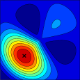
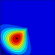
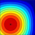
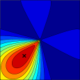
$p_{\theta}=0$ $q_{\theta}=-\pi/8,\forall q\in\mathcal{Q}$

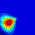
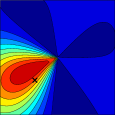
Figure 2: Patch maps for different parametrizations and kernels. We present two parametrizations in polar and two in cartesian coordinates, with absolute or relative gradient angle for each one. The similarity between each pixel of patch $\mathcal{Q}$ and a single pixel $p$ is shown over patch $\mathcal{Q}$. All pixels in $\mathcal{Q}$ have the same gradient angle, which is shown in red arrows. The position of pixel $p$ is shown with “$\times$” on the patch maps. We show examples for $\Delta\theta$ equal to $0$ (top) and $\pi/8$ (bottom). At the top of each column the kernels that are used (patch similarity) are shown. The similarity is shown in a relative manner and, therefore, the absolute scale is missing. Ten isocontours are sampled uniformly and shown in different color.

Figure 3: Patch map with polar parametrization $k_{\phi}k_{\rho}k_{\tilde{\theta}}$ for $\Delta\theta=\pi/4$ and the pair of toy pixel and patch on the left. The example explains why the kernel undergoes shifting away from the position of pixel $p$. The diagram of the 4th column overlays pixel $p$ and 3 pixels of patch $\mathcal{Q}$ with the same distance from the center as $p$. On the rightmost plot, we illustrate $k_{\tilde{\theta}}$ ($p_{\tilde{\theta}}$, $q_{\tilde{\theta}}$), $k_{\phi}$ ($p_{\phi}$, $q_{\phi}$) for pixels $q$ with $q_{\rho}=p_{\rho}$ (on the black dashed circle). $k_{\tilde{\theta}}$ is maximized at $q^{(3)}$, $k_{\phi}$ at $q^{(1)}$, and their product at $q^{(2)}$.

&

4.3 Post-processing learned with or w/o supervision.

We detail different ways to learn the projection matrix $A$ of (9) to perform the descriptor post-processing. Let us consider a learning set of patches $\mathbb{P}$ and the corresponding set of descriptors $V_{\mathbb{P}}=\{V(\mathcal{P}),~{}\mathcal{P}\in\mathbb{P}\}$. Let $C$ be the covariance matrix of $V_{\mathbb{P}}$. Vector $\mu$ is the mean descriptor vector, and different ways to compute $A$ are as follows.

Supervised whitening. We further assume that supervision is available in the form of pairs of matching patches. This is given by set $\mathbb{M}=\{(\mathcal{P},\mathcal{Q})\in\mathbb{P}\times\mathbb{P},~{}\mathcal{P}\sim\mathcal{Q}\}$, where $\sim$ denotes matching patches. We follow the work of Mikolajczyk and Matas MM07 to learn discriminative projections using the available supervision. The discriminative projection is composed of two parts, a whitening part and a rotation part. The whitening part is obtained from the intraclass (matching pairs) covariance matrix $C_{\mathbb{M}}$, while the rotation part is the PCA of the interclass (non-matching pairs) covariance matrix in the whitened space. We set the interclass one to be equal to $C$ as this is dominated by non-matching pairs, while the intraclass one is given by

$$C_{\mathbb{M}}=\sum_{(\mathcal{P},\mathcal{Q})\in\mathbb{M}}\left(V(\mathcal{P})-V(\mathcal{Q})\right)\left(V(\mathcal{P})-V(\mathcal{Q})\right)^{\top}.$$ (14)

The projection matrix is now given by

$$A=C_{\mathbb{M}}^{-\nicefrac{{1}}{{2}}}\mbox{eig}(C_{\mathbb{M}}^{-\nicefrac{{1}}{{2}}}CC_{\mathbb{M}}^{-\nicefrac{{1}}{{2}}}),$$ (15)

where eig denotes the eigenvectors of a matrix into columns. To reduce the descriptor dimensionality, only eigenvectors corresponding to the largest eigenvalues are used. The same holds for all cases that we perform PCA in the rest of the paper. We refer to this transformation as supervised whitening (W_S).

Unsupervised whitening. There is no supervision in this case and the projection is learned via PCA on set $V_{\mathbb{P}}$. In particular, projection matrix is given by

$$A=\mbox{eig}(C)\mbox{diag}(\lambda_{1}^{-\nicefrac{{1}}{{2}}},\ldots,\lambda_{d}^{-\nicefrac{{1}}{{2}}})^{\top},$$ (16)

where diag denotes a diagonal matrix with the given elements on its diagonal, and $\lambda_{i}$ is the $i$-th eigenvalue of matrix $C$. This method is called PCA whitening and we denote simply by W JC12 .

Unsupervised whitening with shrinkage. We extend the PCA whitening scheme by introducing parameter $t$ controlling the extent of whitening and the projection matrix becomes

$$A=\mbox{eig}(C)\mbox{diag}(\lambda_{1}^{-\nicefrac{{t}}{{2}}},\ldots,\lambda_{d}^{-\nicefrac{{t}}{{2}}})^{\top},$$ (17)

where $t\in[0,1]$, with $t=1$ corresponding to the standard PCA whitening and $t=0$ to simple rotation without whitening.

Equivalently, $t=0$ imposes the covariance matrix to be identity. We call this method attenuated PCA whitening and denote it by W_UA.

The aforementioned process resembles covariance estimation with shrinkage LW04 ; LW04b . The sample covariance matrix is known to be a noise estimator, especially when the available samples are not sufficient relatively to the number of dimensions LW04b . Ledoit and Wolf LW04b propose to replace this by a linear combination of the sample covariance matrix and a structured estimator. Their solution is well conditioned and is shown to reduce the effect of noisy estimation in eigen decomposition. The imposed condition is simply that all variances are the same and all covariances are zero. The shrunk covariance is

$$\tilde{C}=(1-\beta)C+\beta\mathbf{I}_{d},$$ (18)

where $\mathbf{I}_{d}$ is the identity matrix and $\beta$ the shrinking parameter. This process “shrinks” extreme (too large or too small) eigenvalues to intermediate ones. In our experiments we show that a simple tuning of parameter $\beta$ performs well across different context and datasets. The projection matrix is now

$$\small A=\mbox{eig}(C)\mbox{diag}((\alpha\lambda_{1}+\beta)^{-\nicefrac{{1}}{{2}}},\ldots,(\alpha\lambda_{d}+\beta)^{-\nicefrac{{1}}{{2}}})^{\top},$$ (19)

where $\alpha=1-\beta$. We call this method PCA whitening with shrinkage and denote it by W_US. We set parameter $\beta$ equal to the $i$-th eigenvalue. A method similar to ours is used in the work of Brown et al. BHW11 , but does not allow dimensionality reduction since descriptors are projected back to the original space after the eigenvalue clipping.

4.4 Visualizing and understanding patch similarity.

We define pixel similarity $\mathcal{M}(p,q)$ as kernel response between pixels $p$ and $q$, approximated as $\mathcal{M}(p,q)\approx\psi(p)^{\top}\psi(q)$. To show a spatial distribution of the influence of pixel $p$, we define a patch map of pixel $p$ (fixed $p_{x}$, $p_{y}$, and $p_{\theta}$). The patch map has the same size as the image patches; for each pixel $q$ of the patch, map $\mathcal{M}(p,q)$ is evaluated for some constant value of $q_{\theta}$.

For example, in Figure 4.2 patch maps for different kernels are shown. The position of $p$ is denoted by $\times$ symbol. Then, $p_{\theta}=0$, while $q_{\theta}=0$ for all spatial locations of $q$ in the top row and $q_{\theta}=-\pi/8$ in the bottom row. This example shows the toy patches and their gradient angles in arrows to be more explanatory. The toy patches are directly defined by $p_{\theta}$, and $q_{\theta}$. Only $p_{\theta}$ and $q_{\theta}$ are used in later examples, while the toy patches are skipped from the figures.

The example in Figure 4.2 reveals a discontinuity near the center of the patch when pixel similarity is given by $\mathbf{V}_{\phi\rho\tilde{\theta}}$ descriptor. It is caused by the polar coordinate system where a small difference in the position near the origin causes large difference in $\phi$ and $\tilde{\theta}$. The patch maps reveal weaknesses of kernel descriptors, such the aforementioned discontinuity, but also advantages of each parametrization. It is easy to observe that the kernel parametrized by Cartesian coordinates and absolute angle of the gradient ($\mathbf{V}_{xy\theta}$, third column) is insensitive to small translations, i.e. feature point displacement. Moreover, in the bottom row we see that using the relative gradient direction $\tilde{\theta}$ allows to compensate for imprecision caused by small patch rotation, i.e. the most similar pixel is not the one at the location of $p$ with different $\tilde{\theta}$, but a rotated pixel with more similar value of $\tilde{\theta}$. This effect is further analyzed in Figure 4.2. The final similarity involves the product of two kernels that both depend on angle $\phi$. They are both maximized at the same point if $\Delta\theta=0$, otherwise not. The larger $\Delta\theta$ is, the maximum value moves further (in the patch) from $p$.

We additionally construct patch maps in the case of descriptor post-processing by a linear transformation, e.g. descriptor whitening. Now the contribution of a pixel pair is given by

$$\hat{\mathcal{M}}(p,q) =(A^{\top}(\psi(p)-\mu))^{\top}(A^{\top}(\psi(q)-\mu))$$ (20)

$$=(\psi(p)-\mu)^{\top}AA^{\top}(\psi(q)-\mu)$$

$$=\psi(p)^{\top}AA^{\top}\psi(q)-\psi(p)^{\top}AA^{\top}\mu$$

$$\quad-\psi(q)^{\top}AA^{\top}\mu+\mu^{\top}AA^{\top}\mu.$$

The last term is constant and can be ignored. If $A$ is a rotation matrix then the similiarity is affected just by shifting by $\mu$. After the transformation, the similarity is no longer shift-invariant. Non-linear post-processing, such as power-law normalization or simple $\ell_{2}$ normalization cannot be visualized, as it acts after the pixel aggregation.

$k_{\phi}$ $k_{\rho}$ $k_{\tilde{\theta}}$	$k_{x}$ $k_{y}$ $k_{\theta}$	$k_{\phi}$ $k_{\rho}$ $k_{\tilde{\theta}}$ + $k_{x}$ $k_{y}$ $k_{\theta}$

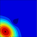
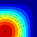
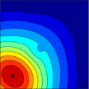
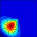
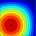
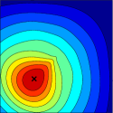
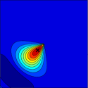
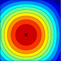
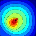
Figure 4: Patch maps for different pixels and parametrizations and their concatenation. We present two parametrizations in polar and Cartesian coordinates, with relative and absolute gradient angle, respectively. $\Delta\theta$ is fixed to be $0$ (individual values of $p_{\theta}$ and $q_{\theta}$ do not matter due to shift invariance) and pixel $p$ is shown with “$\times$”. Note the behaviour around the centre in the concatenated case. Ten isocontours are sampled uniformly and shown in different color.

	PC	P+WS	C+WS	PC+WS	PC+WUA	PC+WUS
$p_{\theta}=0$ $q_{\theta}=0,\forall q\in\mathcal{Q}$
$p_{\theta}=\pi/4$ $q_{\theta}=\pi/4,\forall q\in\mathcal{Q}$
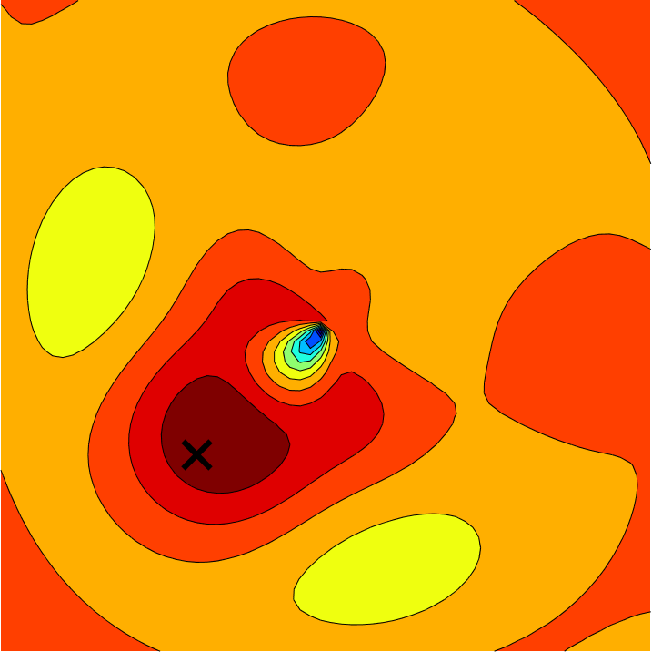
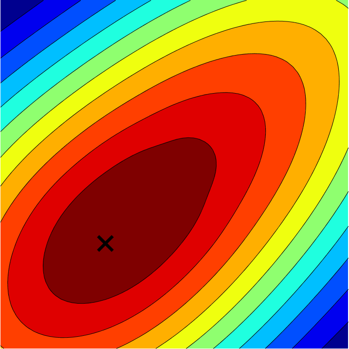
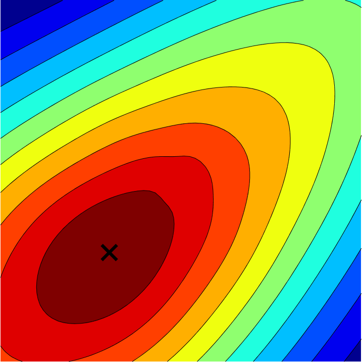
$p_{\theta}=\pi/2$ $q_{\theta}=\pi/2,\forall q\in\mathcal{Q}$
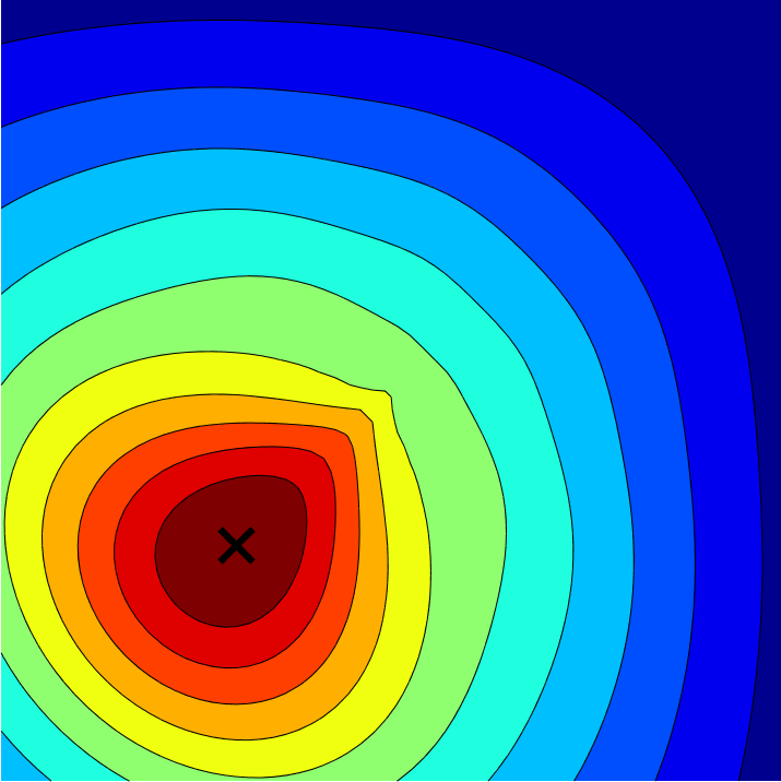
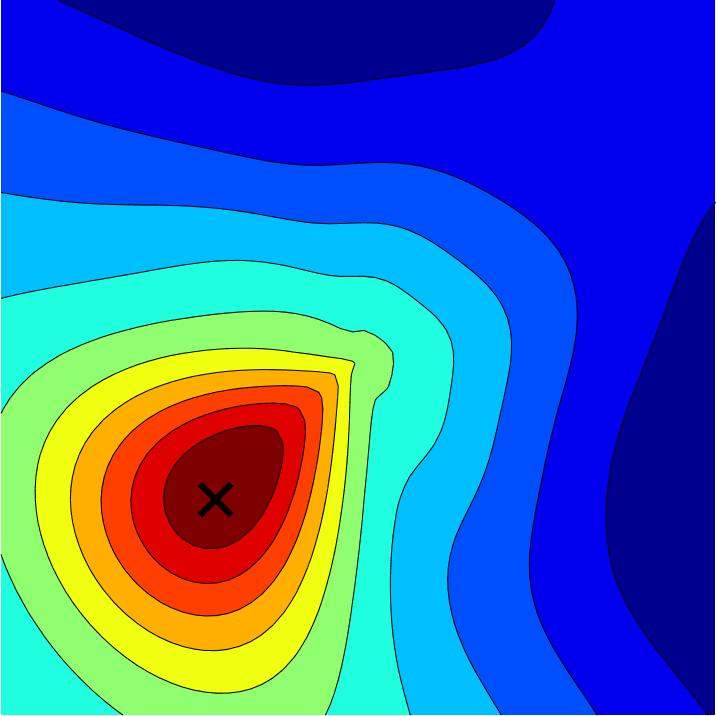
$p_{\theta}=3\pi/4$ $q_{\theta}=3\pi/4,\forall q\in\mathcal{Q}$
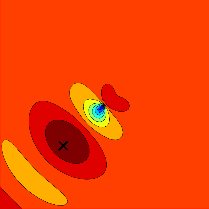
$p_{\theta}=\pi$ $q_{\theta}=\pi,\forall q\in\mathcal{Q}$

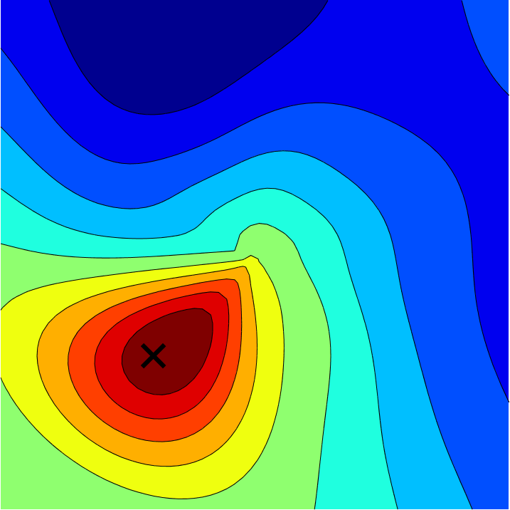
Figure 5: Patch maps for different parametrizations, their concatenation, different post-processing methods, and varying $p_{\theta}$ and $q_{\theta}$, while $\Delta\theta$ is always 0. Pixel $p$ is shown with “$\times$”. P: polar parametrization, C: cartesian parametrization, W_UA is shown for $t=0.7$ and W_US for $\beta=\lambda_{40}$. Whitening is learned on Liberty dataset. Observe that the similarity is no more shift invariant after the whitening and how the shape follows the angle of the gradients. Ten isocontours are sampled uniformly and shown in different color.

Figure 6: Visualizing 1D slices of a patch map. Showing similarity $k(p,q)$ for all pixels $q$ with $q_{x}=p_{x}$ (middle figure) and $q_{y}=p_{y}$ (right figure). It corresponds to 1D similarity across the dashed lines (magenta and blue, respectively) of the patch map on the left. The particular patch map on the left is only chosen as an illustrative example. We show similarity for the first row and for columns 1, 4, 5 and 6 of patch maps from Figure 5. Pixel $p$ has $p_{x}=20$ and $p_{y}=20$ with the origin considered at the bottom left corner.

4.5 Combining kernel descriptors.

We propose to take advantage of both parametrizations $\mathbf{V}_{\phi\rho\tilde{\theta}}$ and $\mathbf{V}_{xy\theta}$, by summing their contribution. This is performed by simple concatenation of the two descriptors. Finally, whitening is jointly learned and dimensionality reduction is performed.

In Figure 4 we show patch maps for the individual and combined representation, for different pixels $p$. Observe how the combined one better behaves around the center. The combined descriptor inherits reasonable behavior around the patch center and insensitivity to position misalignment from the Cartesian parametrization, while insensitivity to dominant orientation misalignment from the polar parametrization, as shown earlier.

$\mathcal{Q}$	P	C	PC	PC+WS	$\mathcal{P}$	P	C	PC	PC+WS

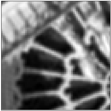
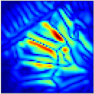
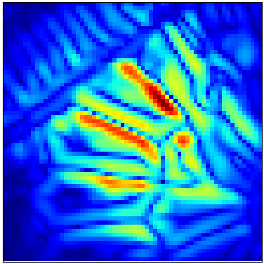
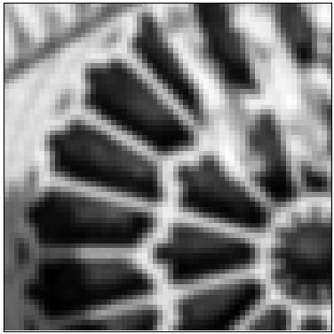
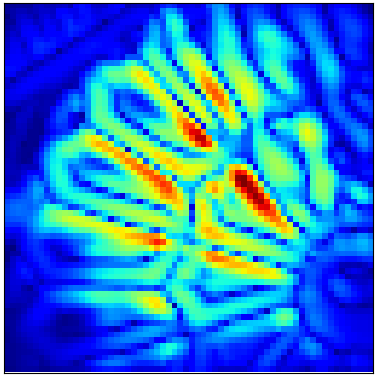
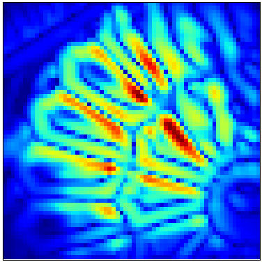
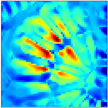
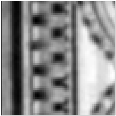
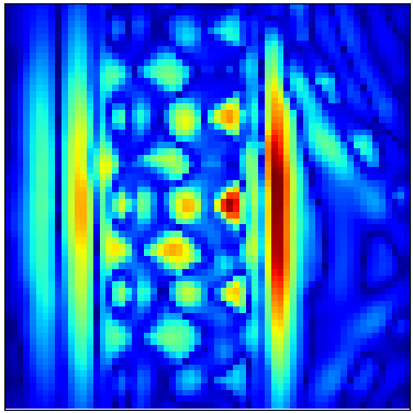
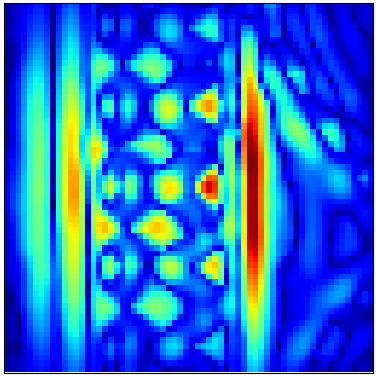
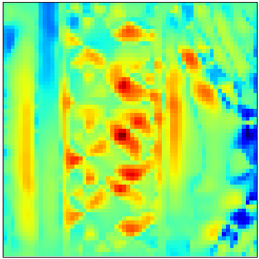
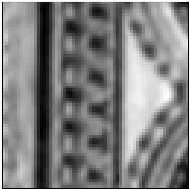
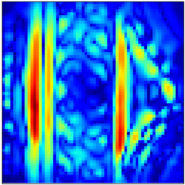
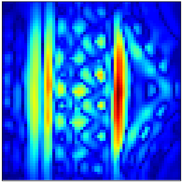
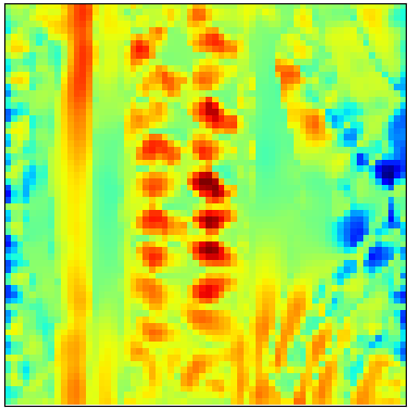
Figure 7: Positive patch pairs (patches $\mathcal{Q}$ and $\mathcal{P}$) and the corresponding heat maps for polar (P), Cartesian (C), combined (PC), and whitened combined (PC+W_S) parametrization. Red (blue) corresponds to maximum (minimum) value. Heat maps on the left side correspond to $\sum_{p\in\mathcal{P}}\mathcal{M}(p,q)$, while the ones on the right side to $\sum_{q\in\mathcal{Q}}\mathcal{M}(p,q)$. In the case of PC+W_S, $\hat{\mathcal{M}}(p,q)$ is used instead of $\mathcal{M}(p,q)$.

4.6 Understanding the whitened patch similarity.

We learn the different whitening variants of Section 4.3 and visualize their patch maps in Figure 5. All examples shown are for $\Delta\theta=0$ but gradient angles $p_{\theta}$ and $q_{\theta}$ jointly vary. We initially observe that the similarity is shift invariant only in the fist column of patch maps where no whitening is applied. This is expected by definition. Projecting by matrix $A$ does not allow to reconstruct the shift invariant kernels anymore; the similarity does not only depend on $\Delta\theta$, which is 0, but also on $p_{\theta}$ and $q_{\theta}$.

The patch similarity learned by whitening exhibits an interesting property. The shape of the 2D similarity becomes anisotropic and gets aligned with the orientation of the gradient. Equivalently, it becomes perpendicular to the edge on which the pixel lies. This is a semantically meaningful effect. It prevents over-counting of pixel matching along aligned edges of the two patches. In the case of a blob detector this can provide tolerance to errors in the scale estimation, i.e. the similarity remains large towards the direction that the blob edges shift in case of scale estimation error.

We presume that this is learned by pixels with similar gradient angle that co-occur frequently. A similar effect is captured by both the supervised and the unsupervised whitening with covariance shrinkage, it is, though, less evident in the case of W_US. Moreover, we see that it is mostly the Cartesian parametrization that allows this kind of deformation.

According to our interpretation, supervised whitening MM07 ; RTC16 owes its success to covariance estimation that is more noise free. The noise removal comes from supervision, but we show that standard approaches for well-conditioned and accurate covariance estimation have similar effect on the patch similarity even without supervision. The observation that different parametrizations allow for different types of co-occurrences to be captured is related to other domains too. For instance. CNN-based image retrieval exhibits improvements after whitening BL15 , but this is very unequal between average and max pooling. However, observing the differences is not as easy as in our case with the visualized patch similarity.

Finally, we obtain slices from the 2D patch maps and present the 1D similarity kernels in Figure 6. It is the similarity between pixel $p$ and all pixels $q\in\mathcal{Q}$ that lie on the vertical and horizontal lines drawn on the patch map at the left of Figure 6. We present the case for which $p_{\theta}=0$ and $q_{\theta}=0,\forall q\in\mathcal{Q}$ (top row in Figure 5). The gradient angle is fully horizontal in this case and the 2D similarity kernel tends to get aligned with that, while the chosen slices are aligned in this fashion too. In our experiments we show that all W_S, W_UA, and W_US provide significant performance improvements. However, herein, we observe that the underlined patch similarity demonstrates some differences. Supervised whitening W_S is not a decreasing function, which might be an outcome of over-fitting to the training data. This is further validated in our experiments. Finally, W_UA and W_S are not maximized on point $p$, which does not seem a desired property. W_US is maximized similarly to the raw descriptor without any post-processing.

Patch maps are a way to visualize and study the general shape of the underlined similarity function. In a similar manner, we visualize the kernel responses for a particular pair of patches to reflect which are the pixels contributing the most to the patch similarity. This is achieved by assigning strength $\sum_{q\in\mathcal{Q}}\hat{\mathcal{M}}(p,q)$ to pixel $p$. In cases without whitening, $\mathcal{M}(p,q)$ is used. We present such heat maps in Figure 7. Whitening significantly affects the contribution of most pixels. The over-counting phenomenon described in Section 4.6 is also visible; some of the long edges are suppressed.

&

Figure 8: Impact of the shrinkage parameter for unsupervised whitening when trained on the same or different dataset. We evaluate performance on Photo Tourism and HPatches datasets versus shrinkage parameter $t$ for the attenuated whitening W_UA (top row), and versus shrinkage parameter $\beta=\lambda_{i}$ for whitening with shrinkage W_US (bottom row).

5 Experiments

We evaluate our descriptor on two benchmarks, namely the widely used Phototourism (PT) dataset WB07 , and the recently released HPatches (HP) dataset BLVM17 . We first show the impact of the shrinkage parameters in unsupervised whitening, and then compare with the baseline method of Bursuc et al. BTJ15 on top of which we build our descriptor. We examine the generalization properties of whitening when learned on PT but tested on HP, and finally compare against state-of-the-art descriptors on both benchmarks. In all our experiments with descriptor post-processing the dimensionality is reduced to 128, while the combined descriptor original has 238 dimensions, except for the cases where the input descriptor is already of lower dimension. Our experiments are conducted with a Matlab implementation of the descriptor, which takes 5.6 ms per patch for extraction on a single CPU on a 3.5GHz desktop machine. A GPU implementation reduces time to 0.1 ms per patch on an Nvidia Titan X.

5.1 Datasets and protocols.

The Phototourism dataset contains three sets of patches, namely, Liberty (Li), Notredame (No) and Yosemite (Yo). Additionally, labels are provided to indicate the 3D point that the patch corresponds to, thereby providing supervision. It has been widely used for training and evaluating local descriptors. Performance is measured by the false positive rate at 95% of recall (FPR95). The protocol is to train on one of the three sets and test on the other two. An average over all six combinations is reported.

The HPatches dataset contains local patches of higher diversity, is more realistic, and during evaluation the performance is measured on three tasks: verification, retrieval, and matching. We follow the standard evaluation protocol BLVM17 and report mean Average Precision (mAP). We follow the common practice and use models learned on Liberty of PT to compare descriptors that have not used HP during learning. We evaluate on all 3 train/test splits and report the average performance. All reported results on HP (our and other descriptors) are produced by our own evaluation by using the provided framework, and descriptors.

Figure 9: Eigenvalues for standard PCA whitening, attenuated whitening ($t=0.7$) and whitening with shrinkage ($\beta=\lambda_{40}$). We normalize so that the maximum eigenvalue is 1. First 120 eigenvalues (out of 238) are shown.

5.2 Impact of the shrinkage parameter.

We evaluate the impact of the shrinkage parameter involved in the unsupervised whitening. It is $t$ for W_UA and $\beta=\lambda_{i}$ for W_US. Results are presented in Figure 4.2 for evaluation on PT and HP dataset, while the whitening is learned on the same or different dataset. The performance is stable for a range of values, which makes it easy to tune in a robust way across cases and datasets. In the rest of our experiments we set $t=0.7$ and $\beta=\lambda_{40}$. In Figure 9 we show the eigenvalues used by W, W_UA, and W_US. The contrast between the larger and smaller eigenvalues is decreased.

$Test$			Liberty		Notredame		Yosemite
$Train$	$D$	$Mean$	$No$	$Yo$	$Li$	$Yo$	$Li$	$No$
${\it polar}\text{~{}\cite[cite]{\@@bibref{Authors Phrase1YearPhrase2}{BTJ15}{\@@citephrase{(}}{\@@citephrase{)}}}}$	$175$	$22.42$	$24.34$	$24.34$	$16.06$	$16.06$	$26.85$	$26.85$
${\it cartes}$	$63$	$35.87$	$34.06$	$34.06$	$34.10$	$34.10$	$39.47$	$39.47$
${\it polar}+{\it cartes}$	$238$	$25.37$	$26.16$	$26.16$	$20.04$	$20.04$	$29.91$	$29.91$
${\it polar}+PCA+SQRT\text{~{}\cite[cite]{\@@bibref{Authors Phrase1YearPhrase2}{BTJ15}{\@@citephrase{(}}{\@@citephrase{)}}}}$	$128$	$8.30$	$12.09$	$13.13$	$5.16$	$5.41$	$7.52$	$6.49$
${\it polar}\text{~{}\cite[cite]{\@@bibref{Authors Phrase1YearPhrase2}{BTJ15}{\@@citephrase{(}}{\@@citephrase{)}}}}+W\textsubscript{S}$	$128$	$7.06$	$8.55$	$10.48$	$4.40$	$3.94$	$8.86$	$6.12$
${\it cartes}+W\textsubscript{S}$	$63$	$15.13$	$17.31$	$20.34$	$10.90$	$11.85$	$16.84$	$13.55$
${\it polar}+{\it cartes}+W\textsubscript{S}$	$128$	$\bf{5.94}$	$\bf{7.46}$	$\bf{9.85}$	$\bf{3.45}$	$\bf{3.55}$	$6.47$	$\bf{4.89}$
${\it polar}+{\it cartes}+W\textsubscript{UA}$	$128$	$6.79$	$10.59$	$11.17$	$3.80$	$4.36$	$\bf{5.58}$	$5.16$
${\it polar}+{\it cartes}+W\textsubscript{US}$	$128$	$7.22$	$10.61$	$11.14$	$4.27$	$4.46$	$6.75$	$6.09$

Table 1: Performance comparison on Phototourism dataset between the baseline approach and our combined descriptor. We further show the benefit of learned whitening (W_S) over the standard PCA followed by square-rooting, as well as the other variants that do additional regularization (W_UA, W_US) without supervision. FPR95 is reported for all methods.

Figure 10: Histograms of patch similairity for positive and negative patch pairs. Histograms are constructed from 50K matching and 50K non-matching pairs from Notredame dataset.

$Name$	$Train$	$Sup.$	$R$	$M$	$V$
${\it polar}+{\it cartes}$	$N/A$	$N/A$	$45.23$	$29.68$	$77.78$
${\it polar}+{\it cartes}+W\textsubscript{UA}$	$PT$	$No$	$52.78$	$36.46$	$77.31$
${\it polar}+{\it cartes}+W\textsubscript{US}$	$PT$	$No$	53.50	37.16	78.81
${\it polar}+{\it cartes}+W\textsubscript{S}$	$PT$	$Yes$	$49.66$	$32.58$	$75.82$
${\it polar}+{\it cartes}+W\textsubscript{UA}$	$HP$	$No$	$56.36$	$39.88$	$80.06$
${\it polar}+{\it cartes}+W\textsubscript{US}$	$HP$	$No$	$56.71$	$40.13$	$80.70$
${\it polar}+{\it cartes}+W\textsubscript{S}$	$HP$	$Yes$	61.79	44.40	83.50

Table 2: Generalization of different whitening approaches. Mean Average Precision(mAP) for 3 tasks of HP, namely Retrieval (R), Matching (M), and Verification (V). The whitening is learned on PT or HP. We denote supervised by Sup.

5.3 Comparison with the baseline.

We compare the combined descriptor against the different parametrizations when used alone. The experimental evaluation is shown in Table 1 for the PT dataset. The baseline is followed by PCA and square-rooting, as originally proposed in  BTJ15 . We did not consider the square-rooting variant in our analysis in Section 4 because such non-linearity does not allow to visualize the underlined patch similarity. Supervised whitening on top of the combined descriptor performs the best. Unsupervised whitening significantly improves too, while it does not require any labeling of the patches.

Polar parametrization with the relative gradient direction (polar) significantly outperforms the Cartesian parametrization with the absolute gradient direction (cartes). After the descriptor post-processing (polar + W_S vs. cartes + W_S), the gap is reduced. The performance of the combined descriptor (polar + cartes) without descriptor post-processing is worse than the baseline descriptor. That is caused by the fact, that the two descriptors are combined with an equal weight, which is clearly suboptimal. No attempt is made to estimate the mixing parameter explicitly. It is implicitly included in the post-processing stage (see Appendix A).

Figure 10 presents patch similarity histograms for matching and non-matching pairs, showing how their separation is improved by the final descriptor.

We perform an experiment with synthetic patch transformations to test the robustness of different parametrizations. The whole patch is synthetically rotated or translated by appropriately transforming pixel position and gradient angle in the case of rotation. A fixed amount of rotation/translation is performed for one patch of each pair of the PT dataset and results are presented in Figure 4.2. It is indeed verified that the Cartesian parametrization is more robust to translations, while the polar one to rotations. The joint one finally partially enjoys the benefits of both.

Figure 11: Performance on PT (training on Liberty , testing on Notredame) when one patch of each pair undergoes synthetic rotation or translation.

5.4 Generalization of whitening.

We learn the whitening on PT or HP (supervised and unsupervised) and evaluate the performance on HP. We present results in Table 2. Whitening always improves the performance of the raw descriptor. The unsupervised variant is superior when learning it on an independent dataset. It generalizes better, implying over-fitting of the supervised one (recall the observations of Figure 6). Learning on HP (the corresponding training part per split) with supervision significantly helps. Note that PT contains only patches detected by DoG, while HP uses a combination of detectors.

5.5 Comparison with the State of the Art.

We compare the performance of the proposed descriptor with previously published results on Phototourism dataset. Results are shown in Table 3. Our method obtains the best performance among the unsupervised/hand-crafted approaches by a large margin. Overall, it comes right after the two very recent CNN-based descriptors, namely L2Net TW17 and HardNet MMR+17 . The advantage of our approach is the low cost of the learning. It takes less than a minute; about 45 seconds to extract descriptors of Liberty and about 10 seconds to compute the projection matrix. CNN-based competitors require several hours or days of training.

The comparison on the HPatches dataset is reported in Figure 4.2. We use the provided descriptors and framework to evaluate all approaches by ourselves. For the descriptors that require learning, the model that is learned on Liberty-PT is used. Our unsupervised descriptor is the top performing hand-crafted variant by a large margin. Overall, it is always outperformed by HardNet, L2Net, while on verification is it additionally outperformed by DDesc and TF-M. Verification is closer to the learning task (loss) involved in the learning of these CNN-based methods.

Finally, we learn supervised whitening W_S for all other descriptors, post-process them, and present results in Figure 4.2. The projection matrix is learned on HP, in particular the training part of each split. Supervised whitening W_S consistently boosts the performance of all descriptors, while this comes at a minimal extra cost compared to the initial training of a CNN descriptor. Our descriptor comes 3rd at 2 out of 3 tasks. Note that it uses the whitening learned on HP (similarly to all other descriptors of this comparison), but does not use the PT dataset at all. All CNN-based descriptors train their parameters on Liberty-PT which is costly, while the overall learning of our descriptor is again in the order of a single minute.

Supervised $Name$ $D$ $FPR@95$ $Brown~{}\emph{et al.}\text{~{}\cite[cite]{\@@bibref{Authors Phrase1YearPhrase2}{BHW11}{\@@citephrase{(}}{\@@citephrase{)}}}}$ $29-36$ $15.36$ $Trzcinski~{}\emph{et al.}\text{~{}\cite[cite]{\@@bibref{Authors Phrase1YearPhrase2}{TCL+12}{\@@citephrase{(}}{\@@citephrase{)}}}}$ $128$ $17.08$ $Simonyan~{}\emph{et al.}\text{~{}\cite[cite]{\@@bibref{Authors Phrase1YearPhrase2}{SVZ13}{\@@citephrase{(}}{\@@citephrase{)}}}}$ $73-77$ $10.38$ $DC-S2S\text{~{}\cite[cite]{\@@bibref{Authors Phrase1YearPhrase2}{ZK15}{\@@citephrase{(}}{\@@citephrase{)}}}}$ $512$ $9.67$ $DDESC\text{~{}\cite[cite]{\@@bibref{Authors Phrase1YearPhrase2}{STFK+15}{\@@citephrase{(}}{\@@citephrase{)}}}}$ $128$ $9.85$ $Matchnet\text{~{}\cite[cite]{\@@bibref{Authors Phrase1YearPhrase2}{HLJS+15}{\@@citephrase{(}}{\@@citephrase{)}}}}$ $4096$ $7.75$ $TF-M\text{~{}\cite[cite]{\@@bibref{Authors Phrase1YearPhrase2}{BRPM16}{\@@citephrase{(}}{\@@citephrase{)}}}}$ $128$ $6.47$ $L2Net+\text{~{}\cite[cite]{\@@bibref{Authors Phrase1YearPhrase2}{TW17}{\@@citephrase{(}}{\@@citephrase{)}}}}$ $128$ $2.22$ $HardNet+\text{~{}\cite[cite]{\@@bibref{Authors Phrase1YearPhrase2}{MMR+17}{\@@citephrase{(}}{\@@citephrase{)}}}}$ $128$ ${\bf 1.51}$ ${\it polar}+{\it cartes}+W\textsubscript{S}~{}(our)$ $128$ $5.98$

Unsupervised $Name$ $D$ $FPR@95$ $RootSIFT$ $128$ $26.14$ $RootSIFT+PCA+SQRT\text{\cite[cite]{\@@bibref{Authors Phrase1YearPhrase2}{BTJ15}{\@@citephrase{(}}{\@@citephrase{)}}}}$ $80$ $17.51$ ${\it polar}+PCA+SQRT\text{\cite[cite]{\@@bibref{Authors Phrase1YearPhrase2}{BTJ15}{\@@citephrase{(}}{\@@citephrase{)}}}}$ $128$ $8.30$ ${\it polar}+{\it cartes}+W\textsubscript{UA}~{}(our)$ $128$ ${\bf 6.79}$ ${\it polar}+{\it cartes}+W\textsubscript{US}~{}(our)$ $128$ $7.21$

Table 3: Performance comparison with the state of the art on Phototourism dataset. We report FPR@95 averaged over 6 dataset combinations for supervised (left) and unsupervised (right) approaches. The whitening for our descriptor is learned on the corresponding training part of PT for each combination.

Figure 12: Performance comparison on HP benchmark. The learning, whenever applicable, is performed on Liberty of PT dataset. Descriptors that do not require any supervision in the form of labeled patches, i.e. hand-crafted or unsupervised, are shown in striped bars. Our descriptor is denoted by PCW_US (P=polar, C=cartes).

Figure 13: Performance comparison on HP benchmark when post-processing all descriptors with supervised whitening W_S which is learned on HP. The initial learning of the descriptor, whenever applicable, is performed on Liberty of PT dataset. Our descriptor uses the whitening learned on HP and does not use the PT dataset at all. Our descriptor is denoted by PCW_S (P=polar, C=cartes).

6 Conclusions

We have proposed a multiple-kernel local-patch descriptor combining two parametrizations of gradient position and direction. Each parametrization provides robustness to a different type of patch miss-registration: polar parametrization for noise in the dominant orientation, Cartesian for imprecise location of the feature point. We have performed descriptor whitening and have shown that its effect on patch similarity is semantically meaningful. The lessons learned from analyzing the similarity after whitening can be exploited for further improvements of kernel, or even CNN-based, descriptors. Learning the whitening in a supervised or unsupervised way boosts the performance. Interestingly, the latter generalizes better and sets the best so far performing hand-crafted descriptor that is competing well even with CNN-based descriptors. Unlike the currently best performing CNN-based approaches, the proposed descriptor is easy to implement and interpret.

7 Acknowledgments

The authors were supported by the OP VVV funded project CZ.02.1.01/0.0/0.0/16_019/0000765 “Research Center for Informatics” and MSMT LL1303 ERC-CZ grant. Arun Mukundan was supported by the CTU student grant SGS17/185/OHK3/3T/13. We would like to thank Karel Lenc and Vassileios Balntas for their valuable help with the HPatches benchmark, and Dmytro Mishkin for providing the L2Net and HardNet descriptors for the HPatches dataset.

Appendix A Regularized concatenation

When combining the descriptors of different parametrization by concatenation we use both with equal contribution, i.e. the final similarity is equal to $k_{\phi}k_{\rho}k_{\tilde{\theta}}+k_{x}k_{y}k_{\theta}$. In the case of the raw descriptors this is clearly suboptimal. One would rather regularize by $k_{\phi}k_{\rho}k_{\tilde{\theta}}+wk_{x}k_{y}k_{\theta}$ and search for the optimal value of scalar $w$. We are about to prove that this is not necessary in the case of post-processing by supervised whitening, where the optimal regularization is included in the projection matrix.

We denote a set of descriptors without regularized concatenation by $V_{\mathbb{P}}$ when $w=1$, while the $V_{\mathbb{P}}^{(w)}$ when $w\neq 1$. It holds that $V_{\mathbb{P}}^{(w)}=\{WV(\mathcal{P}),~{}\mathcal{P}\in\mathbb{P}\}$, where $W$ is a diagonal matrix with ones on the dimensions corresponding to the first descriptors (for $k_{\phi}$ $k_{\rho}$ $k_{\tilde{\theta}}$), and has all the rest elements of the diagonal equal to $w$. The covariance matrix of $V_{\mathbb{P}}$ is $C$, while of $V_{\mathbb{P}}^{(w)}$ it is $C^{(w)}=WCW^{\top}$.

Learning the supervised whitening on $V_{\mathbb{P}}$ as in (15) produces projection matrix

$$A=C_{\mathbb{M}}^{-\nicefrac{{1}}{{2}}}\mbox{eig}(C_{\mathbb{M}}^{-\nicefrac{{1}}{{2}}}CC_{\mathbb{M}}^{-\nicefrac{{1}}{{2}}}),$$ (21)

while learning it on $V_{\mathbb{P}}^{(w)}$ produces projection matrix

$$A^{(w)}={C_{\mathbb{M}}^{(w)}}^{-\nicefrac{{1}}{{2}}}\mbox{eig}({C_{\mathbb{M}}^{(w)}}^{-\nicefrac{{1}}{{2}}}C^{(w)}{C_{\mathbb{M}}^{(w)}}^{-\nicefrac{{1}}{{2}}}).$$ (22)

Cholesky decomposition of $C$ gives

$$C=U^{\top}U=LL^{\top},$$ (23)

which leads to the Cholesky decomposition

$$C^{(w)}=WU^{\top}UW^{\top}=WLL^{\top}W^{\top}.$$ (24)

Using (24) allows us to rewrite (22) as

$$A^{(w)} ={(L^{\top}W^{\top})}^{-1}\mbox{eig}({(WU^{\top})}^{-1}WCW^{\top}{(L^{\top}W^{\top})}^{-1})$$ (25)

$$={(W^{\top})}^{-1}{(L^{\top})}^{-1}\mbox{eig}({U^{\top}}^{-1}W^{-1}WCW^{\top}(W^{\top})^{-1}{(L^{\top})}^{-1})$$

$$={(W^{\top})}^{-1}{(L^{\top})}^{-1}\mbox{eig}({U^{\top}}^{-1}C{(L^{\top})}^{-1})$$

$$={(W^{\top})}^{-1}{(L^{\top})}^{-1}\mbox{eig}(C_{\mathbb{M}}^{-\nicefrac{{1}}{{2}}}CC_{\mathbb{M}}^{-\nicefrac{{1}}{{2}}})$$

$$={(W^{\top})}^{-1}A$$

.

Whitening descriptor $V(\mathcal{P})\in V_{\mathbb{P}}$ with matrix $A$ is performed by

$$\hat{V}(\mathcal{P})=A^{\top}(V(\mathcal{P})-\mu),$$ (26)

while whitening descriptor ${V(\mathcal{P})}^{(w)}\in V_{\mathbb{P}}^{(w)}$ with matrix $A^{(w)}$ is performed by

$${\hat{V}(\mathcal{P})}^{(w)} ={A^{(w)}}^{\top}(WV(\mathcal{P})-W\mu)$$ (27)

$$=A^{\top}{W}^{-1}(WV(\mathcal{P})-W\mu)$$

$$=\hat{V}(\mathcal{P}).$$

No matter what the regularization parameter is, the descriptor is identical after whitening. We conclude that there is no need to perform such regularized concatenation.

References

- (1) Ahonen, T., Matas, J., He, C., Pietikäinen, M.: Rotation invariant image description with local binary pattern histogram fourier features. In: Scandinavian Conference on Image Analysis, pp. 61–70. Springer (2009)
- (2) Alahi, A., Ortiz, R., Vandergheynst, P.: Freak: Fast retina keypoint. In: CVPR (2012)
- (3) Ambai, M., Yoshida, Y.: Card: Compact and real-time descriptors. In: ICCV (2011)
- (4) Arandjelovic, R., Zisserman, A.: Three things everyone should know to improve object retrieval. In: CVPR (2012)
- (5) Babenko, A., Lempitsky, V.: Aggregating deep convolutional features for image retrieval. In: ICCV (2015)
- (6) Balntas, V., Johns, E., Tang, L., Mikolajczyk, K.: Pn-net: conjoined triple deep network for learning local image descriptors. In: arXiv (2016)
- (7) Balntas, V., Lenc, K., Vedaldi, A., Mikolajczyk, K.: Hpatches: A benchmark and evaluation of handcrafted and learned local descriptors. In: CVPR (2017)
- (8) Balntas, V., Riba, E., Ponsa, D., Mikolajczyk, K.: Learning local feature descriptors with triplets and shallow convolutional neural networks. In: BMVC (2016)
- (9) Bau, D., Zhou, B., Khosla, A., Oliva, A., Torralba, A.: Network dissection: Quantifying interpretability of deep visual representations. In: CVPR, pp. 3319–3327. IEEE (2017)
- (10) Bay, H., Ess, A., Tuytelaars, T., Van Gool, L.: Speeded-up robust features (SURF). CVIU 110(3), 346–359 (2008)
- (11) Bo, L., Ren, X., Fox, D.: Kernel descriptors for visual recognition. In: NIPS (2010)
- (12) Bo, L., Ren, X., Fox, D.: Depth kernel descriptors for object recognition. In: IROS (2011)
- (13) Bo, L., Sminchisescu, C.: Efficient match kernels between sets of features for visual recognition. In: NIPS (2009)
- (14) Brown, M., Hua, G., Winder, S.: Discriminative learning of local image descriptors. IEEE Trans. PAMI 33(1), 43–57 (2011)
- (15) Brown, M., Szeliski, R., Winder, S.: Multi-image matching using multi-scale oriented patches. In: CVPR, vol. 1, pp. 510–517 (2005)
- (16) Bursuc, A., Tolias, G., Jégou, H.: Kernel local descriptors with implicit rotation matching. In: ICMR (2015)
- (17) Calonder, M., Lepetit, V., Strecha, C., Fua, P.: Brief: Binary robust independent elementary features. In: ECCV (2010)
- (18) Chum, O.: Low dimensional explicit feature maps. In: ICCV (2015)
- (19) Delhumeau, J., Gosselin, P.H., Jégou, H., Pérez, P.: Revisiting the VLAD image representation. In: ACM Multimedia (2013)
- (20) Dong, J., Soatto, S.: Domain-size pooling in local descriptors: Dsp-sift. In: CVPR (2015)
- (21) Forssén, P.E., Lowe, D.G.: Shape descriptors for maximally stable extremal regions. In: Computer Vision, 2007. ICCV 2007. IEEE 11th International Conference on, pp. 1–8. IEEE (2007)
- (22) Frahm, J.M., Fite-Georgel, P., Gallup, D., Johnson, T., Raguram, R., Wu, C., Jen, Y.H., Dunn, E., Clipp, B., Lazebnik, S., et al.: Building rome on a cloudless day. In: ECCV (2010)
- (23) Han, X., Leung, T., Jia, Y., Sukthankar, R., Berg, A.C.: Matchnet: Unifying feature and metric learning for patch-based matching. In: CVPR (2015)
- (24) Heikkila, M., Pietikainen, M., Schmid, C.: Description of interest regions with local binary patterns. Pattern recognition 42(3), 425–436 (2009)
- (25) Heinly, J., Schonberger, J.L., Dunn, E., Frahm, J.M.: Reconstructing the world* in six days*(as captured by the yahoo 100 million image dataset). In: CVPR (2015)
- (26) Jaderberg, M., Simonyan, K., Zisserman, A., et al.: Spatial transformer networks. In: NIPS, pp. 2017–2025 (2015)
- (27) Jégou, H., Chum, O.: Negative evidences and co-occurrences in image retrieval: The benefit of PCA and whitening. In: ECCV (2012)
- (28) Ke, Y., Sukthankar, R.: PCA-SIFT: a more distinctive representation for local image descriptors. In: CVPR, pp. 506–513 (2004)
- (29) Kokkinos, I., Yuille, A.: Scale invariance without scale selection. In: CVPR (2008)
- (30) Lazebnik, S., Schmid, C., Ponce, J.: A sparse texture representation using local affine regions. IEEE Trans. PAMI 27(8), 1265–1278 (2005)
- (31) Ledoit, O., Wolf, M.: Honey, i shrunk the sample covariance matrix. The Journal of Portfolio Management 30(4), 110–119 (2004)
- (32) Ledoit, O., Wolf, M.: A well-conditioned estimator for large-dimensional covariance matrices. Journal of multivariate analysis 88(2), 365–411 (2004)
- (33) Leutenegger, S., Chli, M., Siegwart, R.Y.: Brisk: Binary robust invariant scalable keypoints. In: ICCV (2011)
- (34) Lowe, D.G.: Distinctive image features from scale-invariant keypoints. IJCV 60(2), 91–110 (2004)
- (35) Mahendran, A., Vedaldi, A.: Visualizing deep convolutional neural networks using natural pre-images. IJCV 120(3), 233–255 (2016)
- (36) Mairal, J., Koniusz, P., Harchaoui, Z., Schmid, C.: Convolutional kernel networks. In: NIPS, pp. 2627–2635 (2014)
- (37) Mikolajczyk, K., Matas, J.: Improving descriptors for fast tree matching by optimal linear projection. In: ICCV (2007)
- (38) Mikolajczyk, K., Schmid, C.: A performance evaluation of local descriptors. IEEE Trans. PAMI 27(10), 1615–1630 (2005)
- (39) Mishchuk, A., Mishkin, D., Radenovic, F., Matas, J.: Working hard to know your neighbor’s margins: Local descriptor learning loss. In: NIPS (2017)
- (40) Mishkin, D., Matas, J., Perdoch, M., Lenc, K.: Wxbs: Wide baseline stereo generalizations. In: arXiv (2015)
- (41) Mukundan, A., Tolias, G., Chum, O.: Multiple-kernel local-patch descriptor. In: BMVC (2017)
- (42) Ojala, T., Pietikainen, M., Maenpaa, T.: Multiresolution gray-scale and rotation invariant texture classification with local binary patterns. IEEE Trans. PAMI 24(7), 971–987 (2002)
- (43) Oliva, A., Torralba, A.: Modeling the shape of the scene: a holistic representation of the spatial envelope. IJCV 42(3), 145–175 (2001)
- (44) Paulin, M., Douze, M., Harchaoui, Z., Mairal, J., Perronin, F., Schmid, C.: Local convolutional features with unsupervised training for image retrieval. In: ICCV (2015)
- (45) Paulin, M., Mairal, J., Douze, M., Harchaoui, Z., Perronnin, F., Schmid, C.: Convolutional patch representations for image retrieval: an unsupervised approach. ICCV 121(1), 149–168 (2017)
- (46) Philbin, J., Isard, M., Sivic, J., Zisserman, A.: Descriptor learning for efficient retrieval. In: ECCV (2010)
- (47) Radenović, F., Tolias, G., Chum, O.: CNN image retrieval learns from BoW: Unsupervised fine-tuning with hard examples. In: ECCV (2016)
- (48) Rublee, E., Rabaud, V., Konolige, K., Bradski, G.: Orb: An efficient alternative to sift or surf. In: ICCV (2011)
- (49) van de Sande, K.E.A., Gevers, T., Snoek, C.G.M.: Evaluating color descriptors for object and scene recognition. IEEE Trans. PAMI 32(9), 1582–1596 (2010)
- (50) Schmid, C., Mohr, R.: Local grayvalue invariants for image retrieval. IEEE Trans. PAMI 19(5), 530–535 (1997)
- (51) Schonberger, J.L., Frahm, J.M.: Structure-from-motion revisited. In: CVPR (2016)
- (52) Schönberger, J.L., Hardmeier, H., Sattler, T., Pollefeys, M.: Comparative evaluation of hand-crafted and learned local features. In: CVPR (2017)
- (53) Schönberger, J.L., Radenović, F., Chum, O., Frahm, J.M.: From single image query to detailed 3D reconstruction. In: CVPR (2015)
- (54) Scovanner, P., Ali, S., Shah, M.: A 3-dimensional sift descriptor and its application to action recognition. In: Proceedings of the 15th ACM International Conference on Multimedia, pp. 357–360 (2007)
- (55) Shechtman, E., Irani, M.: Matching local self-similarities across images and videos. In: CVPR, pp. 1–8. IEEE (2007)
- (56) Simo-Serra, E., Trulls, E., Ferraz, L., Kokkinos, I., Fua, P., Moreno-Noguer, F.: Discriminative learning of deep convolutional feature point descriptors. In: ICCV (2015)
- (57) Simonyan, K., Vedaldi, A., Zisserman, A.: Learning local feature descriptors using convex optimisation. IEEE Trans. PAMI 36(8), 1573–1585 (2014)
- (58) Taira, H., Torii, A., Okutomi, M.: Robust feature matching by learning descriptor covariance with viewpoint synthesis. In: ICPR (2016)
- (59) Tian, B.F.Y., Wu, F.: L2-net: Deep learning of discriminative patch descriptor in euclidean space. In: CVPR (2017)
- (60) Tola, E., Lepetit, V., Fua, P.: Daisy: An efficient dense descriptor applied to wide-baseline stereo. IEEE Trans. PAMI 32(5), 815–830 (2010)
- (61) Tolias, G., Bursuc, A., Furon, T., Jégou, H.: Rotation and translation covariant match kernels for image retrieval. CVIU 140, 9–20 (2015)
- (62) Trzcinski, T., Christoudias, M., Lepetit, V., Fua, P.: Learning image descriptors with the boosting-trick. In: NIPS (2012)
- (63) Vedaldi, A., Zisserman, A.: Efficient additive kernels via explicit feature maps. In: CVPR (2010)
- (64) Vedaldi, A., Zisserman, A.: Efficient additive kernels via explicit feature maps. IEEE Trans. PAMI 34, 480–492 (2012)
- (65) Wang, P., Wang, J., Zeng, G., Xu, W., Zha, H., Li, S.: Supervised kernel descriptors for visual recognition. In: CVPR (2013)
- (66) Winder, S., Brown, M.: Learning local image descriptors. In: CVPR (2007)
- (67) Yi, K.M., Trulls, E., Lepetit, V., Fua, P.: Lift: Learned invariant feature transform. In: ECCV, pp. 467–483. Springer (2016)
- (68) Yosinski, J., Clune, J., Nguyen, A., Fuchs, T., Lipson, H.: Understanding neural networks through deep visualization. arXiv preprint arXiv:1506.06579 (2015)
- (69) Yu, G., Morel, J.M.: A fully affine invariant image comparison method. In: ICASSP, pp. 1597–1600. IEEE (2009)
- (70) Zagoruyko, S., Komodakis, N.: Learning to compare image patches via convolutional neural networks. In: CVPR (2015)
- (71) Zeiler, M.D., Fergus, R.: Visualizing and understanding convolutional networks. In: ECCV (2014)
- (72) Zhou, L., Zhu, S., Shen, T., Wang, J., Fang, T., Quan, L.: Progressive large scale-invariant image matching in scale space. In: ICCV (2017)