Dissipative entanglement preparation via Rydberg antiblockade and Lyapunov control

Abstract

Preparation of entangled steady states via dissipation and pumping in Rydberg atoms has been recently found to be useful for quantum information processing. The driven-dissipative dynamics is closely related to the natural linewidth of the Rydberg states and can be usually modulated by engineering the thermal reservior. Instead of modifying the effectively radiative decay, we propose an alternatively optimized scheme, which combines the resonant Rydberg antiblockade excitation and the Lyapunov control of the ground states to speed up the prepration of the singlet state for two interacting Rydberg atoms. The acceleration process strongly depends on the initial state of the system with respect to the initial coherence between the singlet state and decoherence-sensitive bright state. We study the optimal parameter regime for fast entanglement preparation and the robustness of the fidelity against random noises. The numerical results show that a fidelity above 0.99 can be achieved around 0.4 ms with the current experimental parameters. The scheme may be generalized for preparation of more complicate multi-atom entangled states.

I Introduction

Rydberg atoms are considered the ideal architecture for quantum information processing since it provides strongly interatomic interaction on demand and keeps a radiative lifetime as long as tens of microseconds allowing for laser addressing GallagherTF_1994 ; Low_PB2012 ; Saffman_RMP2010 ; Vogt_PRL2006 ; Tong_PRL2004 ; Dudin_Science2012 . Despite continuous experimental progress in enhancing the Rydberg-ground coupling, it has been demonstrated that the spontaneous emission of the high-lying excited states still causes non-negligible detrimental effects in preparation of atomic entangled states Plenio_PRA1999 ; Cabrillo_PRA1999 ; Schneider_PRA2002 ; Braun_PRL2002 ; Jakobczyk_PRA2002 ; ShaoXQ_a_PRA2017 ; Su_PRA2015 , construction of quantum logic gate Jaksch_PRL2000-1 ; Su_PRA2016 ; Wu_PRA2017-1 ; Wu_PRA2010-1 , and engineering of many-body quantum dynamics Dudin_NP2012 via Rydberg mediated interactions. Instead of protecting the Rydberg open system against atomic decay induced decoherence, there have been several studies CarrAW_PRL2013 ; Bhaktavatsala RaoDD_PRL2013 ; ChenX_PRA2017 ; ShaoXQ_PRA2014 ; LeeS_NJP2015 ; ShaoXQ_b_PRA2017 ; ChenX_PRA2018 , which proposed to use dissipation as a resource by Rydberg pumping. Among these proposals, Rydberg states are excited by using a single-photon excitation or a two-photon excitation process, and the general tasks of quantum information processing can be realized generally in a long time limit. Because of that, more recent interests have centered around speeding up the pumping-dissipative dynamics toward the desired steady state. Some first attempts have been proposed by engineering the radiative decay with an artificial reservoir Bhaktavatsala RaoDD_PRA2014 .

Optimal control techniques can usually provide efficient and operational algorithms for dynamical control of quantum systems HouSC_PRA2012 . Independently of the type of quantum architecture, the general paradigm for quantum control is guiding the quantum dynamics to attain the desired state by engineering the system’s Hamiltonian WangX_PRL2011 . One of the useful control approaches is the Lyapunov-based control (see HouSC_PRA2012 ; WangX_IEEE2010 ; KuangS_Automatica2008 ; KuangS_AAS2010 ; MirrahimiM_Automatica2005 ; GrivopoulosS_IEEE2003 ; VettoriP_LAIA2002 ; ShiZC_PRA2015 ; WangX_PRA2009 ; CuiW_PRA2013 ; WangX_PRA2010 ; YiXX_PRA2009 ; WangW_PRA2010 and the references herein), which consists of using Lyapunov functions to generate trajectories and open-loop steering control, and has the advantage of being simple to handle for rigorous analysis. Successful applications of the Lyapunov control have been found in control of single-particle systems in decoherence-free subspace YiXX_PRA2009 ; WangW_PRA2010 , preparation of few-atom entangled states in the context of cavity quantum electrodynamics WangX_PRA2009 ; CuiW_PRA2013 ; RanD_PRA2017 ; ChenYH_PRA2017 ; ChenYH_PRA2018 , state transfer along the spin chains ShiZC_PRA2015 ; WangX_PRA2010 , as well as dynamical oscillation of macroscopic objects HouSC_PRA2012 . In general, the dynamical evolution can be accelerated to resist the system’s decoherence induced by the photon leakage and photon scattering.

In this paper, we propose a dissipation-based scheme to prepare the two-atom singlet state by modifying the Rydberg antiblockade condition and the coherent unitary dynamics via Lyapunov control. We first compensate Rydberg interactions induced level shift by the two-photon detuning of an optical excitation laser, the Stark shifts caused by which further matches the microwave driving frequency. By making use of the atomic spontaneous emission as a resource and adding target-state-tracking fields to coherently control the driven-dissipative process, we finally generate a unique steady singlet state with high fidelity. Compared to the previous studies, we have further examined the effect of the Stark shifts induced by the dispersive coupling between the ground state and the Rydberg state, which is found to be important for the driven-dissipative dynamics. By canceling out the Stark shifts with a detuned microwave field or an auxiliary dispersive laser, the level configuration of the two-atom system can be effectively regarded as a five-level resonant interaction system. Therefore, it is not difficult to exactly solve the coherent evolution dynamics, which provides the hints for optimal control, e.g., by appropriately selecting the optimal frequency and driving strength of the microwave field, the converging to the target state can be much faster than that with other choices. On the other hand, the driven-dissipative dynamics towards the decoherence-free state is further accelerated by using the method of Lyapunov control, which leads to a fidelity of higher than 0.99 around 0.4 ms. In general, our scheme gives an example for fast dissipative preparation of singlet state for two Rydberg atoms via the Lyapunov control, and more importantly, it would be helpful for understanding the details of the Rydberg-ground interaction dynamics under the drivings of an optical laser and a microwave field, which is significant for understanding the Rydberg-interaction-mediated many-body dynamics.

The paper is organized as follows: In section 2, we derive the effective Hamiltonian for the atoms suffering from antiblockade Rydberg interactions and introduce the basic scheme for dissipative preparation of two-atom singlet state. In section 3, the Lyapunov control method and its application in speeding up the dissipative state preparation is discussed in detail. The improved scheme under the Lyapunov control is numerically studied in section 4, where we consider the effect of the system initial state, atomic spontaneous emission, and the control parameters on the converging process. In section 5, the experimental feasibility and the robustness against the random fluctuation in parameters are further discussed. Finally, we summarize our results in section 6.

II Rydberg antiblockade and effective model

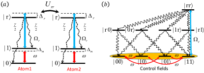
Figure 1: (Color online) (a) Diagram illustration of the atomic-level configuration. The Rydberg state $|r\rangle$ is excited from the ground state $|1\rangle$ by an optical laser with Rabi frequency $\Omega_{r}$ and detuning $\Delta_{r}$. The ground state transition $|0\rangle\leftrightarrow|1\rangle$ is driven by a microwave field with Rabi frequency $\Omega_{m}$ and detuning $\Delta_{m}$. Double excitation of the Rydberg state $|r\rangle$ is shifted by $U_{rr}$ due to the interatomic interaction. Moreover, we assume the Rydberg state spontaneously decays into the two ground states at the same rate $\gamma/2$. (b) Effective level configuration for the two-atom system and atomic transitions among the collective states. The coherent evolution is restrained in the collective-state subspace spanned by $|00\rangle$, $|01\rangle$, $|10\rangle$, $|11\rangle$, and $|rr\rangle$, see main text for the detail.

We consider a system consisting of two identical Rydberg atoms, each of them has two ground states $|0\rangle$, $|1\rangle$ and one Rydberg excited state $|r\rangle$, as shown in Fig.1(a). The transition $|1\rangle\leftrightarrow|r\rangle$ is driven by a classical optical laser with Rabi frequency $\Omega_{r}$ and detuning $\Delta_{r}$, while the transition $|0\rangle\leftrightarrow|1\rangle$ is driven by a microwave field (or alternatively by a two-photon Raman transition) with Rabi frequency $\Omega_{m}$ and detuning $\Delta_{m}$. A dipole-dipole interaction between the atoms arises from the simultaneous excitation of two atoms to the Rydberg state, and the strength $U_{rr}$ of the Rydberg-mediated interaction depends on the interatomic distance and the principal quantum number of the Rydberg state. The Rydberg population spontaneously decays onto the ground states $|0\rangle$ and $|1\rangle$ with the same rate $\gamma/2$ due to the finite radiative lifetime. The Hamiltonian for the system, in the interaction picture, is given by ($\hbar=1$)

$$H=H_{l}+H_{m},$$ (1)

with

$$H_{l}=\frac{1}{2}\sum_{j=1,2}(-\Delta_{r}|r\rangle_{j}\langle r|+\Omega_{r}|r\rangle_{j}\langle 1|+H.c.)+U_{rr}|rr\rangle\langle rr|,$$

$$H_{m}=\frac{1}{2}\sum_{j=1,2}(\Delta_{m}|0\rangle_{j}\langle 0|+\Omega_{m}|1\rangle_{j}\langle 0|)+H.c..$$

While consider the decoherence effect induced by atomic spontaneous emissions, the dissipative dynamics of the system is then governed by the Lindblad-Markovian master equation, i.e.

$$\stackrel{{\scriptstyle.}}{{\rho}} = -i[H,\rho]+\mathcal{L}[\rho],$$ (2)

with

$$\mathcal{L}[\rho]=\sum_{j=1,2}\sum_{k=0,1}L_{j,k}\rho L_{j,k}^{\dagger}-\frac{1}{2}(L_{j,k}^{\dagger}L_{j,k}\rho+\rho L_{j,k}^{\dagger}L_{j,k}),$$

where $\rho$ is the density operator of the system and $L_{j,k}=\sqrt{\gamma/2}|k\rangle_{j}\langle r|$ ($k=0,1$) are Lindblad dissipation operators.

In the regime of the Rydberg antiblockade (namely, $U_{rr}=2\Delta_{r}$) and in the limit of the large detuning $\Delta_{r}\gg\Omega_{r}$, the two atoms tend to be excited in bunching under the laser driving. Then, we can derive an effective Hamiltonian for the system by using the time averaging method James_CJP2007 ,

$$H^{\prime} = 2\Delta_{m}|00\rangle\langle 00|+\frac{\Omega_{r}^{2}}{2\Delta_{r}}(|11\rangle+|rr\rangle)(\langle 11|+\langle rr|)$$ (3)

$$+(\Delta_{m}+\frac{\Omega_{r}^{2}}{4\Delta_{r}})(|01\rangle\langle 01|+|10\rangle\langle 10|)$$

$$+\frac{\Omega_{m}}{2}[(|11\rangle+|00\rangle)(\langle 01|+\langle 10|)+H.c.],$$

where the basis states in the single excitation subspace are adiabatically eliminated. We note that the dispersive coupling not only enables the two-photon atomic transition to the doubly excitation state $|rr\rangle$, but also introduces the Stark shifts $\sim\Delta_{r}^{-1}$ to the collective ground states $|01\rangle$, $|10\rangle$, and $|11\rangle$. Thus, the degeneracy in the ground state subspace is broken, namely, a resonant driving with microwave fields to the individual atomic transition $|0\rangle\leftrightarrow|1\rangle$ is not in resonance with both the collective transitions $|01\rangle(|10\rangle)\leftrightarrow|00\rangle$ and $|01\rangle(|10\rangle)\leftrightarrow$$|11\rangle$ any more. The coherent population transfer among the collective ground states becomes less efficient.

To cancel out the effect of the Stark shifts, it is convenient to introduce a finite detuning $\Delta_{m}=\Omega_{r}^{2}/4\Delta_{r}$ for the microwave driving. In this case, the Hamiltonian (3) in the rotating frame with respect to $\Omega_{r}^{2}/2\Delta_{r}$ reduces to

$$H_{e}=\frac{\Omega_{m}}{\sqrt{2}}(|11\rangle+|00\rangle)\langle B|+\frac{\Omega_{e}}{2}|11\rangle\langle rr|+H.c.,$$ (4)

where $\Omega_{e}=\Omega_{r}^{2}/\Delta_{r}$ and $|B\rangle=(|01\rangle+|10\rangle)/\sqrt{2}$. Alternatively, we can utilize a laser field, dispersively coupling $|1\rangle$ to the an auxiliary state and introduce a energy correction $-\Omega_{r}^{2}/\Delta_{r}$ to the state $|1\rangle$, which leads to the effective Hamiltonian in Eq. (4) as well. For convenience, we further define

$$a = \sqrt{\Omega_{m}^{2}+\left(\frac{\text{$\Omega_{e}$}}{2}\right)^{2}},$$

$$b^{2} = \sqrt{\Omega_{m}^{4}+\left(\frac{\text{$\Omega_{e}$}}{2}\right)^{4}},$$ (5)

$$c = \sqrt{\Omega_{m}^{2}+\frac{\Omega_{e}^{2}}{2}},$$

then the eigenstates of the Hamiltonian (4) without normalization are given by

$$|\phi_{1}\rangle \sim |10\rangle-|01\rangle$$

$$|\phi_{2}\rangle \sim [-2c^{2}\sqrt{a^{2}+b^{2}}+2(a^{2}+b^{2})^{\frac{3}{2}}]|00\rangle$$

$$+ [2\Omega_{m}(a^{2}+b^{2})-\Omega_{m}\Omega_{e}^{2}]|B\rangle$$

$$+ 2\sqrt{a^{2}+b^{2}}\Omega_{m}^{2}|11\rangle+\sqrt{2}\Omega_{m}^{2}\Omega_{e}|rr\rangle$$

$$|\phi_{3}\rangle \sim [-2c^{2}\sqrt{a^{2}-b^{2}}+2(a^{2}-b^{2})^{\frac{3}{2}}]|00\rangle$$

$$+ [2\Omega_{m}(a^{2}-b^{2})-\Omega_{m}\Omega_{e}^{2}]|B\rangle$$

$$+ 2\sqrt{a^{2}-b^{2}}\Omega_{m}^{2}|11\rangle+\sqrt{2}\Omega_{m}^{2}\Omega_{e}|rr\rangle$$

$$|\phi_{4}\rangle \sim [2c^{2}\sqrt{a^{2}+b^{2}}-2(a^{2}+b^{2})^{\frac{3}{2}}]|00\rangle$$

$$+ [2\Omega_{m}(a^{2}+b^{2})-\Omega_{m}\Omega_{e}^{2}]|B\rangle$$

$$- 2\sqrt{a^{2}+b^{2}}\Omega_{m}^{2}|11\rangle+\sqrt{2}\Omega_{m}^{2}\Omega_{e}|rr\rangle$$

$$|\phi_{5}\rangle = [2c^{2}\sqrt{a^{2}-b^{2}}-2(a^{2}-b^{2})^{\frac{3}{2}}]|00\rangle\rangle$$

$$+ [2\Omega_{m}(a^{2}-b^{2})-\Omega_{m}\Omega_{e}^{2}]|B\rangle$$

$$- 2\sqrt{a^{2}-b^{2}}\Omega_{m}^{2}|11\rangle+\sqrt{2}\Omega_{m}^{2}\Omega_{e}|rr\rangle$$

which are associated with the eigenvalues

$$E_{1}=0,\textrm{ }E_{2,3}=\frac{1}{\sqrt{2}}\sqrt{a^{2}\pm b^{2}},\textrm{ }E_{4,5}=-\frac{1}{\sqrt{2}}\sqrt{a^{2}\pm b^{2}},$$ (6)

respectively. Thus, the instantaneous state of the system under the coherent evolution can be written as the superposition of the five eigenstates, namely

$$|\psi(t)\rangle=\sum_{k=1}^{5}C_{k}(t)|\phi_{k}\rangle.$$ (7)

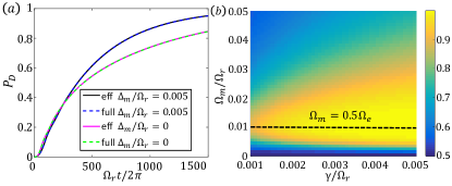
Figure 2: (Color online) (a) Population of the singlet state $P_{D}=\textrm{Tr}[\rho(t)|D\rangle\langle D|]$ as a function of rescaled time with the system initially being in $(|00\rangle+|01\rangle+|10\rangle+|11\rangle)/\sqrt{2}$. The time evolution governed by the effective Hamiltonian (4) agrees well with that dominated by the originally full Hamiltonian (1). The microwave driving with a slight detuning gives rise to a faster convergence to the target state compared with that under resonant driving. (b) $P_{D}$ versus the Rabi frequency $\Omega_{m}$ of the microwave driving and the spontaneous emission rate $\gamma$ of the Rydberg state for $\Omega_{r}t/2\pi=1500$. The optimal driving scheme for the microwave field is found for $\Omega_{m}=0.5\Omega_{e}$. Other parameters are $(\Delta_{r},\gamma,\Omega_{m})/\Omega_{r}=(50,0.002,0.01)$ in (a) and $(\Delta_{r},\Delta_{m})/\Omega_{r}=(50,0.005)$ in (b) in units of $\Omega_{r}=1$.

It has been clearly shown that there exists a unique dark state $|D\rangle=\frac{1}{\sqrt{2}}(|10\rangle-|01\rangle)$, which is also referred to as the two-atom singlet state, corresponding to the null eigenvalue of the system Hamiltonian (1). We now turn to the scheme for preparation of the singlet state by considering and taking advantage of the atomic spontaneous emission.

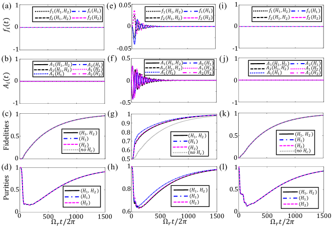
Figure 3: (Color online) Control functions $f_{j}(t)$ [Eq.(11)], matrix elements $A_{j}$ ($j=1,2$), the fidelity and purity of the target state $|D\rangle$ versus dimensionless time for the atoms initially being in the state $|00\rangle$ [(a)-(d)], $|10\rangle$ [(e)-(h)], $|11\rangle$ [(i)-(l)]. The system is subject to three different control manners: (1) $H_{1}\neq 0$, $H_{2}=0$, (2) $H_{1}=0$, $H_{2}\neq 0$, and (3) $H_{1}\neq 0$, $H_{2}\neq 0$, respectively. Other parameters are $(\Delta_{r},\gamma,\Omega_{m},\Delta_{m},\lambda_{1},\lambda_{2})/\Omega_{r}=(50,0.002,0.01,0.005,0.08,0.08)$ in units of $\Omega_{r}=1$.

The schematic diagram for preparing the singlet state is shown in Fig. 1(b), where the collective level configuration consists of four ground states $|00\rangle$, $|01\rangle$, $|10\rangle$, $|11\rangle$, four single-excitation states $|0r\rangle$, $|1r\rangle$, $|r0\rangle$, $|r1\rangle$, and a doubly excitation state $|rr\rangle$. Without the optical excitation of the Rydberg state, the two-atom system will stay in the subspace spanned by {$|00\rangle$, $|B\rangle$, $|11\rangle$} under the microwave driving $H_{m}$. While the optical laser is applied, only when the system populates the state $|11\rangle$ will it be excited to the doubly Rydberg state $|rr\rangle$ (i.e. the Rydberg pumping process), which then decays onto the single-excitation subspace followed by re-occupation of the ground states. Based on the effective Hamiltonian (4), the driven-dissipative dynamics can now be described by

$$\overset{\cdot}{\rho} = -i\left[H_{e},\rho\right]+\mathcal{\widetilde{L}}[\rho]$$ (8)

with $\widetilde{L}_{j,k}=\sqrt{\gamma/2}|k\rangle_{j}\langle r|\otimes\mathcal{I}_{j^{\prime}\neq j}$ ($j$, $j^{\prime}$ $=1$ or 2). It turns out that the singlet state $|D\rangle$ is a decoherence-free state, which is decoupled from any of the driving fields and is the unique steady state solution of the master equation (8), see the example with the initial state $(|00\rangle+|01\rangle+|10\rangle+|11\rangle)/\sqrt{2}$ shown in Fig. 2(a). Mathematically, this can be verified simply by setting $\dot{\rho}=0$ and checking $i\left[H_{e},\rho_{ss}\right]=\mathcal{\widetilde{L}}[\rho_{ss}]$ with $\rho_{ss}$=$|D\rangle\langle D|$. In addition, with the choice of the detuning $\text{$\Delta$}_{m}=\Omega_{r}^{2}/4\Delta_{r}$ and the optimal driving strength $\Omega_{m}=\Omega_{e}/2$ [which corresponds to $a=\sqrt{2}\Omega_{m}$, $b^{2}=\sqrt{2}\Omega_{m}^{2}$, and $c=\sqrt{3}\Omega_{m}$, see Eq. (5)], the system converges to the steady state faster than that with resonant microwave driving. However, this regular driven-dissipative scheme still takes a time as long as $\Omega_{r}t/2\pi\sim 1000$ to achieve a population of the singlet state $P_{D}=\textrm{Tr}[\rho(t)\rho_{ss}]$ larger than 0.9.

III Lyapunov control with microwave fields

The converging process to the steady state can be further accelerated by following the algorithm of the Lyapunov control, which is a method of local optimal control with numerous variants and possesses the advantages of robustness and stability SugawaraM_JCP2003 . To realize an additional control of the system, we first introduce the control Hamiltonian

$$H_{c}=\sum_{j=1,2}f_{j}(t)H_{j},$$ (9)

where $H_{j}=\lambda_{j}|0\rangle_{j}\langle 1|+h.c.$ and the time varying control functions $f_{j}(t)$ are new degree of freedom that allow us to design the system evolution towards the desired state $|D\rangle$. The coherent dynamics of the system is now governed by the quantum Liouville equation $\stackrel{{\scriptstyle.}}{{\rho}}=-i[H_{e}+H_{c},\rho]$. According to the Lyapunov control theory HouSC_PRA2012 ; WangX_IEEE2010 ; KuangS_Automatica2008 ; KuangS_AAS2010 ; MirrahimiM_Automatica2005 ; GrivopoulosS_IEEE2003 ; VettoriP_LAIA2002 ; ShiZC_PRA2015 ; WangX_PRA2009 ; CuiW_PRA2013 ; WangX_PRA2010 ; YiXX_PRA2009 ; WangW_PRA2010 , the control fields $f_{j}(t)$ can be given via pulse shaping of the laser intensities corresponding to a pre-defined Lyapunov function $\xi(t)$, which fulfills the sufficient conditions $\xi(t)\geq 0$ and $\partial_{t}\xi(t)\leq 0$.

In order to describe the converging efficiency of the system under Lyapunov control, we then introduce the time-dependent ’distance’ of the system state away from the target state $S(t)\equiv 1-F(t)\geq 0$, with $F(t)=\langle D|\rho(t)|D\rangle$ refers to the instantaneous fidelity of the target state $|D\rangle$. Moreover, the time-derivative of the ’distance’ $V(t)=\partial_{t}S(t)$ is used for characterizing the instantaneous evolution speed of the driven-dissipative process, leading to HouSC_PRA2012 ; WangX_IEEE2010 ; KuangS_Automatica2008 ; KuangS_AAS2010 ; MirrahimiM_Automatica2005 ; GrivopoulosS_IEEE2003 ; VettoriP_LAIA2002 ; ShiZC_PRA2015 ; WangX_PRA2009 ; CuiW_PRA2013 ; WangX_PRA2010 ; YiXX_PRA2009 ; WangW_PRA2010

$$V(t) = -\langle D|\stackrel{{\scriptstyle\cdotp}}{{\rho}}(t)|D\rangle=V_{a}(t)+V_{b}(t),$$ (10)

with

$$V_{a}(t)=-\sum_{j=1,2}f_{j}(t)\langle D|[-iH_{j},\rho(t)]|D\rangle,$$

$$V_{b}(t)=-\sum_{j,k}\langle D|\widetilde{L}_{j,k}\rho\widetilde{L}_{j,k}^{\dagger}|D\rangle,$$

where we have considered the fact that the decoherence free state $|D\rangle$ is a stationary state satisfying $H_{e}|D\rangle=0$ and $\widetilde{L}_{j,k}|D\rangle=0$. Our main task in the next step is to design a dynamical control that ensures that $S(t)$ is monotonically decreasing until the end of system evolution, which requires $V(t)\leq 0$. Note that the second term in Eq. (10) can be diagonalized in terms of the effective orthonormal excited states {$|E_{m}\rangle$}, giving rise to $V_{b}(t)=-\sum_{m}\gamma_{m}\langle E_{m}|\rho(t)|E_{m}\rangle\leq 0$, with $\gamma_{m}$ being the effective decay rates. Then, if we further set

$$f_{j}(t) = -i\langle D|[H_{j},\rho]|D\rangle$$ (11)

$$= \sqrt{2}\lambda_{j}\textrm{Im}(\langle 11|\rho|D\rangle+\langle D|\rho|00\rangle),$$

it is easy to verify $V_{b}(t)\leq 0$ and $V(t)\leq 0$ with equality only true for the system being initially in $|D\rangle$. With these choices, $S(t)$ becomes exactly the Lyapunov function we are seeking for. Since the control fields $f_{j}(t)$ are target-state-dependent functions and are determined by the elements $A_{1}(t)=\textrm{Im}(\langle 11|\rho|D\rangle),$ $A_{2}(t)=\textrm{Im}(\langle D|\rho|00\rangle)$ of the density matrix, they vanish at the end of dynamical evolution leaving the system in the steady state $|D\rangle$. This time-varying optimization method is also known as trajectory tracking control HouSC_PRA2012 ; WangX_IEEE2010 ; KuangS_Automatica2008 ; KuangS_AAS2010 ; MirrahimiM_Automatica2005 ; GrivopoulosS_IEEE2003 ; VettoriP_LAIA2002 ; ShiZC_PRA2015 ; WangX_PRA2009 ; CuiW_PRA2013 ; WangX_PRA2010 ; YiXX_PRA2009 ; WangW_PRA2010 .

IV Numerical results and discussions

The driven-dissipative dynamics of the system subjected to the Lyapunov control is now dominated by

$$\overset{\cdot}{\rho} = -i\left[H_{e}+H_{c},\rho\right]+\mathcal{\widetilde{L}}[\rho],$$ (12)

based on which, we have shown in Fig. 3 the time-dependent Lyapunov control functions $f_{j}(t)$, the related density matrix elements $A_{j}$ ($j=1,2$), the fidelity $F(t)$ and the purity $P(t)=\text{Tr}(\rho^{2})$ of the system with the atoms initially being in the state $|00\rangle$, $|10\rangle$, and $|11\rangle$, respectively.

We first assume that the system is initially in the state $|\psi(0)\rangle=|00\rangle$. In this case, the fidelity of the singlet state goes through a transient state with $F\approx 0$ and then surpasses $0.9$ at the moment around $\Omega_{r}t/2\pi\sim 1150$, as shown in Fig. 3(a)-3(d). The driven-dissipative dynamics is not accelerated simply because the Lyapunov control cannot be triggered with the matrix elements $\sim A_{1,2}(t)$ of the density operator being zero at all time, i.e. $A_{1,2}(0)\sim\langle D|00\rangle=0$. For the system initially in the state $|\psi(0)\rangle=|11\rangle$, the evolutional dynamics does not exhibit a transient behavior due to the immediate excitation of the Rydberg doubly excitation state. But Similarly, the converging process can not be speeded up due to $A_{1,2}(0)\sim\langle D|11\rangle=0$, see Fig. 3(i)-3(l).

While the system is initially in the state $|\psi(0)\rangle=|10\rangle$ or $|\psi(0)\rangle=|01\rangle$, the Lyapunov control takes effect and the fidelity of larger than 0.9 for the target state can be achieved in a greatly reduced time $\Omega_{r}t/2\pi\sim 600$, as shown in Fig. 3(e)-3(h). Essentially, this is due to the fact that $|10\rangle$ ($|01\rangle$) consists in the coherence between the bright state $|B\rangle$ and the singlet state $|D\rangle$, which is nevertheless non-existent in $|00\rangle$ and $|11\rangle$. To see the insight, we rewrite the initial state $|10\rangle$ as

$$|\psi(0)\rangle=\frac{1}{2}(|B\rangle\langle B|+|D\rangle\langle D|+|D\rangle\langle B|+|B\rangle\langle D|).$$ (13)

Since the bright state $|B\rangle$ under the dominance of the system Hamiltonian (4) coherently couples to both $|00\rangle$ and $|11\rangle$, which immediately transforms the third and fourth terms into the nonvanishing matrix elements $\langle 11|\rho|D\rangle$ and $\langle D|\rho|00\rangle$, activating the self-adaptive control functions [see Eq. (11)]. As the dissipative dynamics evolves and the coherence relaxation between the singlet and the dark state increases, the effect of the Lyapunov control gradually vanishes and finally the conventional driven-dissipative dynamics dominates. We note that the scheme with simply the single-atom Lyapunov control (i.e. $H_{c}=f_{1}(t)H_{1}$ for $|\psi(0)\rangle=|10\rangle$ or $H_{c}=f_{2}(t)H_{2}$ for $|\psi(0)\rangle=|01\rangle$) can even achieve a better converging effect, which arises from the symmetry breaking of the coherent evolution among $|00\rangle$, $|B\rangle$ and $|11\rangle$.

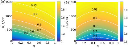
Figure 4: (Color online) Time-dependent fidelity of the singlet state $|D\rangle$ under the Lyapunov control $H_{1}$ for mixed initial states (a) $(1-\eta)|00\rangle\langle 00|+\eta|10\rangle\langle 10|$ and (b) $(1-\eta)|10\rangle\langle 10|+\eta|01\rangle\langle 01|$, respectively. Parameters are $(\Delta_{r},\gamma,\Omega_{m},\Delta_{m},\lambda_{1},\lambda_{2})/\Omega_{r}=(50,0.002,0.01,0.005,0.08,0)$ and $\Omega_{r}=1$.

Moreover, we look into the controlled dynamics with the initial mixed states

$$|\psi(0)\rangle = (1-\eta)|00\rangle\langle 00|+\eta|10\rangle\langle 10|$$ (14)

and

$$|\psi(0)\rangle = (1-\eta)|10\rangle\langle 10|+\eta|01\rangle\langle 01|$$ (15)

$$= \frac{1}{2}(|B\rangle\langle B|+|D\rangle\langle D|)+(\frac{1}{2}-\eta)(|D\rangle\langle B|$$

$$+|B\rangle\langle D|),$$

respectively, see Fig. 4. The former leads to the intuitive result that the converging speed gradually increases as the initial population of the basis state $|10\rangle$ grows. For the latter case, we find that the slowest converging speed appears at $\eta=0.5$, which corresponds to the initial state $\rho(0)=\rho_{BD}\equiv(|B\rangle\langle B|+|D\rangle\langle D|)/2$. Although the population of the bright state $|B\rangle$ and the singlet state $|D\rangle$ for the initial states $|10\rangle\langle 10|$ and $\rho_{BD}$ are the same, the completely mixed state $\rho_{BD}$ does not possess any coherence between them, which inhibits the effect of the control functions and again confirms our prediction with respect to the speed-up conditions.

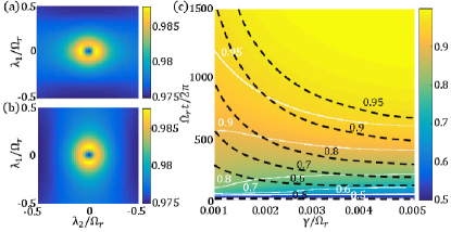
Figure 5: (Color online) Fidelity of the singlet state at time $\Omega_{r}t/2\pi=1500$ as functions of the control parameters $\lambda_{1}$ and $\lambda_{2}$ with the system initially being in $|01\rangle$ [(a)] and $|10\rangle$ [(b)], and as functions of atomic spontaneous emission rate $\gamma/\Omega_{r}$ and dimensionless time $\Omega_{r}t$ [(c)]. In (c), the white (solid) and black (dash) contour lines denote the fidelities with and without Lyapunov control, respectively. Other parameters are the same as in Fig. 4.

Although the additive Lyapunov control can accelerate the preparation of the singlet state, it does not imply that the stronger the driving intensity of the control fields applies the faster the driven-dissipative process converges, which is evidenced in Fig. 5(a)-5(b). For the initial states $|01\rangle$ ($|10\rangle$), the optimized driving strengths appear at $\lambda_{1}=0$, $\lambda_{2}=0.8$ ($\lambda_{1}=0.8$, $\lambda_{2}=0$), which are asymmetric in driving intensities of the two microwave field. Finally, we point out that the acceleration effect strongly depends on the decay rate $\gamma\sim n^{2}$ (or the principal quantum number $n$) of the Rydberg state, as shown in Fig. 5(c). For a slow dissipation process, the Lyapunov control can significantly increase the converging efficiency, e.g., for $\gamma/\Omega_{r}=0.001$, the fidelity of higher 0.9 can be achieved at the time about $1/3$ of that without Lyapunov control. In contrast, only a modest extent of acceleration can be reached for a fast decay for $\gamma/\Omega_{r}\sim 0.005$.

V Experimental feasibility and Influence of the stochastic parameter fluctuations

In the context of experimental feasibility, the schematic energy-level diagram can be encoded by the clock states $|0\rangle=|6S_{1/2},F=3\rangle$, $|1\rangle=|6S_{1/2},F=4\rangle$ and the Rydberg state $|r\rangle=|64P_{3/2}\rangle$ in the ¹³³Cs atoms JauYY_Nature_physics2016 . The transition from the ground state $|1\rangle$ to the Rydberg state $|r\rangle$ is driven by a 390-nm single-photon excitation laser with the Rabi frequency $\Omega_{r}/2\pi\sim 4$ MHz. The dynamical oscillation between the two clock states $|0\rangle$ and $|1\rangle$ is controlled by microwave fields with the coupling strength up to $1$MHz. The decay rate ( or the life time) of the Rydberg state $|r\rangle$ is $\gamma=2\pi\times 0.007$ MHz ($\sim 150\text{ $\mu$}$s). Therefore, the parameter regime we considered is within the reach of the state of the art Rydberg experiments. With respect to the particular case JauYY_Nature_physics2016 , the time required to obtain a high-fidelity $(\text{$\sim$}99\%)$ steady-state entanglement is only about $0.4$ ms.

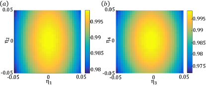
Figure 6: (Color online) Robustness of the steady-state fidelity for $\Omega_{r}t/2\pi=2500$ with respect to stochastic amplitude noise in microwave driving strength ($\eta_{1}$) and frequency ($\eta_{2}$), optical excitation Rabi frequency ($\eta_{3}$), and interatomic interaction ($\eta_{4}$). We assume the initial state of system is $|10\rangle$ and the ideal evolution dynamics is exactly the same to that in Fig. 3(e)-(h) before adding the stochastic noise.

Furthermore, we investigate the influence of stochastic fluctuations in parameters, such as laser intensity $\Omega_{r}$, microwave driving strength $\Omega_{m}$ and detuning $\Delta_{m}$, as well as Rydberg-Rydberg interactions $U_{rr}$ on the steady-state fidelity. To describe the stochastic process, we assumed that the system Hamiltonian is now composed of the coherent part $H_{0}$ and the amplitude-noise part $\eta_{k}\xi(t)H_{sk}$ ($k=1,2,3,4$) with

$$H_{s1} = \frac{\Omega_{m}}{2}\sum_{j=1,2}|0\rangle_{j}\langle 1|+H.c.,$$

$$H_{s2} = \frac{\Delta_{m}}{2}\sum_{j=1,2}|0\rangle_{j}\langle 0|+H.c.,$$

$$H_{s3} = \frac{\Omega_{r}}{2}\sum_{j=1,2}|1\rangle_{j}\langle r|+H.c.,$$

$$H_{s4} = \frac{U_{rr}}{2}|rr\rangle\langle rr|+H.c.,$$ (16)

and $\xi(t)$ being the Gaussian white noise satisfying $\langle\xi(t)\rangle=0$ and $\langle\xi(t)\xi(t^{\prime})\rangle=\delta(t-t^{\prime})$. Starting from an initial pure state $\rho_{\xi}(t=0)$, the stochastic dynamics of the system without involving the atomic decay is governed by

$$\stackrel{{\scriptstyle\cdot}}{{\rho}}_{\xi} = -i[H_{0},\rho_{\xi}]-i\eta[H_{sk},\xi\rho_{\xi}],$$ (17)

which after averaging over the random trajectories becomes Ruschhaupt_NJP2014

$$\stackrel{{\scriptstyle\cdot}}{{\rho}} \simeq -i[H_{0},\rho]-i\eta[H_{sk},\langle\xi\rho_{\xi}\rangle].$$ (18)

Using the Novikov’s theorem, the average of the product of the noise and the noise-dependent density matrix can be further given by $\langle\xi\rho_{\xi}\rangle=\frac{1}{2}\langle\frac{\delta\rho_{\xi}}{\delta\xi(t^{\prime})}\rangle|_{t=t^{\prime}}=-\frac{i\eta}{2}[H_{sk},\rho]$. Therefore, when both the stochastic noise and the atomic dissipation are taken into account, the evolution of the system is finally governed by

$$\stackrel{{\scriptstyle\cdot}}{{\rho}} = -i[H,\rho]+\mathcal{L}[\rho]+\mathbb{\mathbb{\mathcal{D}}}[\rho]$$ (19)

where $\mathbb{\mathbb{\mathcal{D}}}[\rho]=-\eta_{k}^{2}[H_{sk},[H_{sk},\rho]]/2$. Consider the single-atom Lyapunov control $H_{c}=f_{1}(t)H_{1}$ with the control function $f_{1}(t)$ being previously obtained from the dynamics Eq. (12) excluding the noise error, we have shown the steady-state fidelity (at $\Omega_{r}t/2\pi=2500$) as functions of the noise factors $\eta_{k}$ in Fig. 6. It can be found that the steady-state fidelity is reduced by $\sim 2\%$ for $\eta_{1}=0.05$ and $\eta_{3}=0.05$, corresponding to 5% of random fluctuations in the microwave driving intensity and the laser driving strength, respectively. However, the steady-state fidelity is less insensitive to random noise in the microwave detuning $(\sim\eta_{2})$ and the Rydberg-Rydberg interaction strength $(\sim\eta_{4})$.

VI Conclusion

In conclusion, we have proposed the improved dissipation-assisted scheme for preparing the two-atom singlet state under the Rydberg antiblockade and the Lyapunov control. By appropriately selecting the detuning and coupling strength between the microwave driving and the level separation of the two clock states, the system converges to the steady state faster than that with resonant microwave driving. By implementing the Lyapunov control, the system can speed up the convergence if the initial state involves the coherence between the singlet state and the bright state. The improved scheme involving the Lyapunov control is very efficient for a slow dissipative dynamics and becomes less beneficial for a fast decaying system. The scheme may be realized by the state of the art Rydberg experiments and can be potentially generalized to multi-atom scenario.

References

- (1) T. F. Gallagher, Rydberg atoms (Cambridge University Press, Cambridge, 1994).
- (2) R. Löw, H. Weimer, J. Nipper, J. B. Balewski, B. Butscher, H. P. Büchler, and T. Pfau, An experimental and theoretical guide to strongly interacting Rydberg gases, J. Phys. B 45, 113001 (2012).
- (3) M. Saffman, T. G.Walker, and K.Mølmer, Quantum information with Rydberg atoms, Rev. Mod. Phys. 82, 2313 (2010).
- (4) T. Vogt, M. Viteau, J. Zhao, A. Chotia, D. Comparat, and P. Pillet, Dipole blockade at förster resonances in high resolution laser excitation of Rydberg states of cesium atoms, Phys. Rev. Lett. 97, 083003 (2006).
- (5) D. Tong, S. M. Farooqi, J. Stanojevic, S. Krishnan, Y. P. Zhang, R. Cote, E. E. Eyler, and P. L. Gould, Local blockade of Rydberg excitation in an ultracold gas, Phys. Rev. Lett. 93, 063001 (2004).
- (6) Y. O. Dudin and A. Kuzmich, Strongly interacting Rydberg excitations of a cold atomic gas, Science 336, 887 (2012).
- (7) M. B. Plenio, S. F. Huelga, A. Beige, and P. L. Knight, Cavity-loss-induced generation of entangled atoms, Phys. Rev. A 59, 2468 (1999).
- (8) C. Cabrillo, J. I. Cirac, P. García-Fernández, and P. Zoller, Creation of entangled states of distant atoms by interference, Phys. Rev. A 59, 1025 (1999).
- (9) S. Schneider and G. J.Milburn, Entanglement in the steady state of a collective-angular-momentum (Dicke) model, Phys. Rev. A 65, 042107 (2002).
- (10) D. Braun, Creation of entanglement by interaction with a common heat bath, Phys. Rev. Lett. 89, 277901 (2002).
- (11) L. Jakóbczyk, Entangling two qubits by dissipation, J. Phys. A 35, 6383 (2002).
- (12) X. Q. Shao, J. H. Wu, and X. X. Yi, Dissipation-based entanglement via quantum Zeno dynamics and Rydberg antiblockade, Phys. Rev. A 95, 062339 (2017).
- (13) S. L. Su, Q. Guo, H. F. Wang, and S. Zhang, Simplified scheme for entanglement preparation with Rydberg pumping via dissipation, Phys. Rev. A 92, 022328 (2015).
- (14) D. Jaksch, J. I. Cirac, P. Zoller, S. L. Rolston, R. Côté, and M. D. Lukin, Fast quantum gates for neutral atoms, Phys. Rev. Lett. 85, 2208 (2000).
- (15) S. L. Su, E. J. Liang, S. Zhang, J. J. Wen, L. L. Sun, Z. Jin, and A. D. Zhu, One-step implementation of the Rydberg-Rydberg-interaction gate, Phys. Rev. A 93, 012306 (2016).
- (16) H. Wu, X.-R. Huang, C.-S. Hu, Z.-B. Yang, and S.-B. Zheng, Rydberg-interaction gates via adiabatic passage and phase control of driving fields, Phys. Rev. A 96, 022321 (2017).
- (17) H.-Z. Wu, Z.-B. Yang, and S.-B. Zheng, Implementation of a multiqubit quantum phase gate in a neutral atomic ensemble via the asymmetric Rydberg blockade, Phys. Rev. A 82, 034307 (2010).
- (18) Y. O. Dudin, L. Li, F. Bariani, and A. Kuzmich, Observation of coherent many-body Rabi oscillations, Nat. Phys. 8, 790 (2012).
- (19) A. W. Carr and M. Saffman, Preparation of entangled and antiferromagnetic states by dissipative Rydberg pumping, Phys. Rev. Lett. 111, 033670 (2013).
- (20) D. D. Bhaktavatsala Rao and K. Mølmer, Dark entangled steady states of interacting Rydberg atoms, Phys. Rev. Lett. 111, 033606 (2013).
- (21) X. Chen, H. Xie, G. W. Lin, X. Shang, M. Y. Ye, and X. M. Lin, Dissipative generation of a steady three-atom singlet state based on Rydberg pumping, Phys. Rev. A 96, 042308 (2017).
- (22) X. Q. Shao, J. B. You, T. Y. Zheng, C. H. Oh, and S. Zhang, Stationary three-dimensional entanglement via dissipative Rydberg pumping, Phys. Rev. A 89, 052313 (2014).
- (23) S. Lee, J. Cho and K. S. Choi, Emergence of stationary many-body entanglement in driven-dissipative Rydberg lattice gases, New J. Phys. 17 113053 (2015).
- (24) X. Q. Shao, D. X. Li, Y. Q. Ji, J. H. Wu, and X. X. Yi, Ground-state blockade of Rydberg atoms and application in entanglement generation, Phys. Rev. A 96, 012328 (2017).
- (25) X. Chen, G. W. Lin, H. Xie, X. Shang, M. Y. Ye, and X. M. Lin, Fast creation of a three-atom singlet state with a dissipative mechanism and Rydberg blockade, Phys. Rev. A 98, 042335 (2018).
- (26) D. D. Bhaktavatsala Rao and K. Mølmer, Deterministic entanglement of Rydberg ensembles by engineered dissipation, Phys. Rev. A 90, 062319 (2014).
- (27) S. C. Hou, M. A. Khan, X. X. Yi, Daoyi Dong, and Ian R. Petersen, Optimal Lyapunov-based quantum control for quantum systems, Phys. Rev. A 86, 022321 (2012).
- (28) X. Wang, Sai Vinjanampathy, Frederick W. Strauch, and Kurt Jacobs, Ultraefficient cooling of resonators: beating sideband cooling with quantum control, Phys. Rev. Lett. 107, 177204 (2011).
- (29) X. Wang and S. G. Schirmer, Analysis of Lyapunov method for control of quantum states, IEEE Transactions on Automatic Control 55(10), 2259 (2010).
- (30) S. Kuang and S. Cong, Lyapunov control methods of closed quantum systems, Automatica 44, 98 (2008).
- (31) S. Kuang and S. Cong, Optimal Lyapunov-based quantum control for quantum systems, Acta Automat. Sinica 36, 1257 (2010).
- (32) M. Mirrahimi, P. Rouchon, and G. Turinici, Lyapunov control of bilinear Schrödinger equations, Automatica 41, 1987 (2005).
- (33) S. Grivopoulos and B. Bamieh, Lyapunov-based control of quantum systems, in Proceedings of the 42nd IEEE Conference on Decision and Control, Maui, Hawaii., (2003).
- (34) P. Vettori and S. Zampieri, Module theoretic approach to controllability of convolutional systems, Linear Algebra and Its Applications 351, 739 (2002).
- (35) Z. C. Shi, X. L. Zhao, and X. X. Yi, Robust state transfer with high fidelity in spin-1/2 chains by Lyapunov control, Phys. Rev. A 91, 032301 (2015).
- (36) X. Wang and S. G. Schirmer, Entanglement generation between distant atoms by Lyapunov control, Phys. Rev. A 80, 042305 (2009).
- (37) W. Cui and F. Nori, Feedback control of Rabi oscillations in circuit QED, Phys. Rev. A 88, 063823 (2013).
- (38) X. Wang, A. Bayat, S. Bose, and S. G. Schirmer, Global control methods for Greenberger-Horne-Zeilinger-state generation on a one-dimensional Ising chain, Phys. Rev. A 82, 012330 (2010).
- (39) X. X. Yi, X. L. Huang, Chunfeng Wu, and C. H. Oh, Driving quantum systems into decoherence-free subspaces by Lyapunov control, Phys. Rev. A 80, 052316 (2009).
- (40) W. Wang, L. C. Wang, and X. X. Yi, Lyapunov control on quantum open systems in decoherence-free subspaces, Phys. Rev. A 82, 034308 (2010).
- (41) D. Ran, Z. C. Shi, J. Song, Y. Xia, Speeding up adiabatic passage by adding Lyapunov control, Phys. Rev. A 96, 033803 (2017).
- (42) Y. H. Chen, Z. C. Shi, J. Song, Y. Xia, and S. B. Zheng, Coherent control in quantum open systems: An approach for accelerating dissipation-based quantum state generation, Phys. Rev. A 96, 043853 (2017).
- (43) Y. H. Chen, Z. C. Shi, J. Song, Y. Xia, and S. B. Zheng, Accelerated and noise-resistant generation of high-fidelity steady-state entanglement with Rydberg atoms, Phys. Rev. A 97, 032328 (2018).
- (44) Y. Y. Jau, A. M. Hankin, T. Keating, I. H. Deutsch, and G. W. Biedermann, Entangling atomic spins with a Rydberg-dressed spin-flip blockade, Nature Physics 12, 71–74 (2016)
- (45) D. F. V. James and J. Jerke, Effective Hamiltonian theory and its applications in quantum information, Can. J. Phys. 85, 625 (2007).
- (46) M. Sugawara, General formulation of locally designed coherent control theory for quantum system, J. Chem. Phys. 118, 6784 (2003)
- (47) A. Ruschhaupt, X. Chen, D. Alonso, and J. G. Muga, Optimally robust shortcuts to population inversion in two-level quantum systems, New J. Phys. 14, 093404 (2014).