Order Fractionalization

Abstract

The confluence of quantum mechanics and complexity, which leads to the emergence of rich, exotic states of matter, motivates the extension of our concepts of quantum ordering. The twin concepts of spontaneously broken symmetry, described in terms of a Landau order parameter, and of off-diagonal long-range order (ODLRO), are fundamental to our understanding of phases of matter. In electronic matter it has long been assumed that Landau order parameters involve an even number of electron fields, with integer spin and even charge, that are bosons. On the other hand, in low-dimensional magnetism, operators are known to fractionalize so that the excitations carry spin-1/2. Motivated by experiment, mean-field theory and computational results, we extend the concept of ODLRO into the time domain, proposing that in a broken symmetry state, quantum operators can fractionalize into half-integer order parameters. Using numerical renormalization group studies we show how such fractionalized order can be induced in quantum impurity models. We then conjecture that such order develops spontaneously in lattice quantum systems, due to positive feedback, leading to a new family of phases, manifested by a coincidence of broken symmetry and fractionalized excitations that can be detected by experiment.

A major theme in current condensed matter physics is the quest for new types of quantum matter such as high-temperature superconductors, topological insulators and spin liquids Zaanen et al. (2006); Lee et al. (2006); Si et al. (2016); Moore (2010); Qi and Zhang (2011); Hasan and Kane (2010); Savary and Balents (2017); Zhou et al. (2017). An important aspect of this research is the characterization of novel forms of order that emerge in these quantum materials; another concerns the new classes of excitation that accompany these orderings. Landau’s theory of phase transitions Landau (1937) attributes the transformation in macroscopic properties to the development of an order parameter that breaks the microscopic symmetries of the system. Later, Yang observed Yang (1962) that such long-range order is manifested as an asymptotic factorization of spatial correlation functions at long distances into a product of order parameters $\langle{\cal O}(x){\cal O}^{\dagger}(y)\rangle\xrightarrow{|x-y|\rightarrow\infty}\langle{\cal O}(x)\rangle\langle{\cal O}(y)\rangle^{*}$. The quantum operators ${\cal O}$ are bosonic and condense into a state of “Off-Diagonal Long Range Order” (ODLRO).

In relativistic physics half-integer spin order parameters are prohibited by the spin-statistics theorem Pauli (1940); Duck and Sudarshan (1998), but in electronic condensed matter the absence of Lorentz invariance removes this restriction. Though half-integer order can be envisioned in Landau’s theory of phase transitions, it is microscopically incompatible with ODRLO where the local operators that condense are bosons, formed from an even number of half-integer spin fermions. Conventional order parameters such as magnetization or pair density involve pairs of fermions and form part of the general paradigm of BCS/Hartree-Fock order parameters; more complicated “composite order parameters” involving four or more elementary fermion fields have also been envisioned Emery and Kivelson (1992); Balatsky and Boncaa (1993), but all have integer spin. This has led to the implicit assumption that in electronic quantum matter, order parameters satisfy an effective spin-statistics theorem, carrying integer spin and even charge.

Another important development in condensed matter physics is the discovery of “fractionalization”, where the emergent excitations carry fractional quantum numbersWilczek (1982); Fradkin (1991); Laughlin (1983); Anderson (1987). A classic example is the one dimensional spin-$1/2$ Heisenberg antiferromagnet where a spin-flip, that changes the magnetic quantum number by an integer unit, creates a pair of spin-$1/2$ excitations called spinons Tennant et al. (1993); Mourigal et al. (2013). Higher dimensional examples include the fractional quantum Hall effect Laughlin (1983), and spin liquids like the Kitaev honeycomb model where the spin operators fractionalize into Majorana fermions Kitaev (2006). Fractionalization has also been proposed to occur at continuous quantum phase transitions Senthil et al. (2004); Sachdev (2011) leading to “deconfined quantum criticality” where a fluctuating order parameter breaks up into new degrees of freedom. Whereas ODLRO is a ground-state property, fractionalization is associated with excitations, manifested in dynamical response functions and as correlations that are nonlocal in time. In this paper we explore the possible unification of ODLRO and fractionalization, proposing that quantum operators can fractionalize into half-integer order parameters. This order fractionalization conjecture (OFC) requires an extension of ODLRO into space-time, and suggests a new symmetry class of quantum order Wen (2002).

A key setting for our discussion is the Kondo lattice, a model describing an array of magnetic moments interacting via an antiferromagnetic exchange with a sea of conduction electrons. This model is widely used to describe the behavior of heavy fermion materials, where the screening of the magnetic moments by conduction electrons at low temperatures liberates their spins into the Fermi sea as delocalized heavy electrons (Fig. 1A, B), a process that enlarges the Fermi surface. Since a spin flip of a local moment creates a particle-hole pair of heavy fermions, we are led to interpret the expansion of the Fermi surface as a fractionalization of local moments into negatively charged fermions Lebanon and Coleman (2008). The origin of the moments is immaterial and their fractionalization into heavy fermions would even occur if they were of nuclear origin Coleman (2015). (Fig. 1 C).

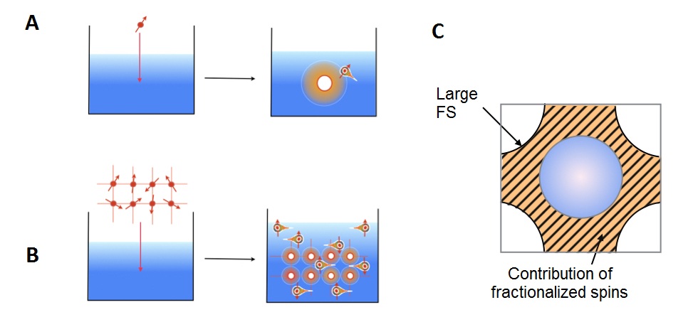
Figure 1: Schematic illustrating the Kondo effect showing (A) the fractionalization of a single spin into a delocalized f-electron in a Kondo impurity model, (B) the fractionalization of local moments in a Kondo lattice, to form a fluid of heavy fermions; (C) the enlargement of the Fermi surface from small (blue) to large (hatched) due to the formation of heavy fermions, as predicted by Oshikawa’s theorem Oshikawa (2000).

There is considerable indirect experimental and theoretical support for spin fractionalization in the Kondo lattice. Using topology, Oshikawa has shown that in a Fermi liquid ground-state, the screened spins of a Kondo lattice contribute to an expansion of its Fermi surface volume Oshikawa (2000). Hall effect and de Haas van Alphen measurements subsequently detected jumps in the Fermi surface volumes at quantum phase transitions between antiferromagnetic and paramagnetic heavy fermion ground-states Paschen et al. (2004); Shishido et al. (2005). The enlargement of the Fermi surface in the Kondo lattice indicates the formation of half-integer excitations from the lattice of local moments, a process that is most naturally interpreted as spin fractionalization.

Experimentally, there are important examples where Kondo spin screening appears coincident with the development of long range order. For instance, in both NpPd₅Al₂ and CeCoIn₅, singlet superconductivity develops directly from a Curie-Weiss paramagnet Aoki et al. (2007); Petrovic et al. (2001) with a substantial loss of spin entropy. Similar phenomenon involving quadrupole degrees of freedom has been proposed for UBe₁₃, URu₂Si₂ and Pr X₂Al₂₀ (X=Ti, Va) Jarrell et al. (1996); Chandra et al. (2013); John S. Van Dyke (2018). Theoretical evidence for spin fractionalization and broken symmetry is found from path-integral based, large-$N$ treatments of Kondo lattices Read and Newns (1983); Coleman et al. (1994, 1999); Flint et al. (2008). However, while these methods demonstrate the feasibility of order fractionalization in models with very large numbers of spin components, they are unable to demonstrate that this phenomenon extends to physical, spin-$1/2$ Kondo lattices. Our motivation to seek new classes of broken symmetry derives from these experimental and theoretical considerations.

Developing this idea, we recall that the dynamics of an interacting fermion is determined by the Dyson self-energy, $\Sigma_{\alpha\beta}(2,1)$, an amplitude for the scattering of a single-particle excitation, a fermion, at space time $1=(x_{1},t_{1})$ back into a single-particle state at the space-time $2\equiv(x_{2},t_{2})$ via intermediate many-body states. Here $\beta$ and $\alpha$ are the internal quantum numbers of the incoming and outgoing fermions. The Hamiltonian that determines the time evolution is invariant under various global symmetry transformations such as spin rotation or global gauge invariance; at high temperatures the self-energy is also invariant under these symmetries. However if a phase transition occurs, the self-energy develops a symmetry-breaking component resulting from scattering off the order parameter. For example a ferromagnet develops a spontaneous Zeeman splitting driven by the internal Weiss field; a BCS superconductor develops a pairing field due to Andreev scattering off the condensate. In all these classical examples, the order parameter has an associated coherence length; for space/times larger than this coherence length, the (coarse-grained) self-energy can be regarded as a local, instantaneous symmetry-breaking potential, $\Sigma_{\alpha\beta}(2,1)=M_{\alpha\beta}(1)\delta(2-1)$, where the order parameter $M_{\alpha\beta}(1)$ transforms as an irreducible representation of the Hamiltonian symmetry group (Fig. 2A).

Fractionalization implies a factorization of quantum operators into two or more independent components. Similarly, we take order fractionalization to imply that at large space-time separations between $1$ and $2$, the self-energy factorizes into a product of fractional order parameters, $\Sigma_{\alpha\beta}(2,1)\sim\bar{V}_{\alpha}(2)V_{\beta}(1)$, where $V_{\beta}(1)$ and $\bar{V}_{\alpha}(2)$ describe a fractional, spinorial order parameter and its conjugate at locations $1$ and $2$, respectively. The independence of these two quantities requires that the intermediate state, which involves an odd number of fermions, develops a bound-state that propagates without decay between $1$ and $2$, as shown schematically in Fig. 2B. Since $V_{\beta}$ carries the quantum number of the incoming fermion, the intermediate bound-state fermion is neutral with respect to this quantum number. This establishes a link between order fractionalization and the formation of neutral fermion bound-states.

Following the example of the Curie-Weiss theory of magnetism, here we develop support for the order fractionalization conjecture. There, the first step is to induce Curie magnetism with an external magnetic field acting on a single spin; next, one argues that in the bulk the interaction of one site on another provides a Weiss field that maintains a spontaneous magnetization Weiss (1907). Similarly here we seek to induce order fractionalization in Kondo impurity models by identifying an appropriate symmetry breaking field. This is a necessary pre-condition for us to argue that “fractionalizing Weiss fields” can spontaneously stabilize order fractionalization in lattices.

Spin Fractionalization. We first identify spin fractionalization in the single impurity Kondo model. Then we show we can induce order fractionalization in the two-channel Kondo impurity model where the local moment is screened by two separate conduction channels. The impurity Kondo model involves an antiferromagnetic spin exchange interaction between a local moment and the spin density of the conduction sea $H_{I}=J(\psi^{\dagger}\vec{\sigma}\psi)\cdot\vec{S}$, where $\psi^{\dagger}$ is a spinor that creates an electron at the site of the impurity. At low energies this model is a resonant level Fermi liquid where the interaction matrix elements behave as an effective (renormalized) Anderson model, $J\psi^{\dagger}(\vec{\sigma}\cdot\vec{S})\psi\rightarrow(\bar{V}\psi^{\dagger}f+Vf^{\dagger}\psi)$. The equivalence of the effective Hamiltonian with its microscopic form implies that the operator combination of a spin and a conduction electron acts as a single, bound-state fermion

$$J(\vec{\sigma}_{\alpha\beta}\cdot\contraction{}{\vec{S}}{)}{\psi}\vec{S})\psi_{\beta}=\bar{V}\hat{f}_{\alpha}.$$ (1)

Here the horizontal line contracting the spin and the fermion implies that at long times, this combination acts as a single composite fermion. Although this process has been amply demonstrated in large-$N$ calculations Read and Newns (1983); Coleman (2007) and is implicitly guaranteed by the low energy equivalence of the Anderson and Kondo impurities models, we now present an explicit demonstration of its occurance in the spin-1/2 Kondo model using numerical renormalization group (NRG) methods Bulla et al. (2008).

In NRG the conduction bath is discretized logarithmically, mapping the model to an impurity spin coupled to a tight-binding (Wilson) chain with exponentially decaying tunneling amplitude. This produces the imaginary part of the Green’s function at a set of discrete frequencies, which are then interpolated to produce a continuous, analytic function satisfying the necessary sum rules. We then transform the T-matrix of the conduction electrons $T(z)$ so obtained, to the irreducible self-energy $\Sigma(z)$ using the relation

$$\Sigma(z)=\frac{T(z)}{1+g(z)T(z)},$$ (2)

where $g(z)$ is the bare local Green’s function of the conduction electrons at the position of the impurity. The unitary single-particle scattering generated by a Kondo singlet at low energies implies that $g(0)T(0)=-1$ at the Fermi energy and hence a singular structure in $\Sigma(z\sim 0)$, making the extraction of $\Sigma(z)$ sensitive to interpolation errors in the NRG. We employ a limiting procedure in which $g(z)\rightarrow(1-\epsilon)g(z)$ , keeping $\epsilon$ larger than the interpolation errors induced in $T(z)$ (c.f. Supplementary Materials A).

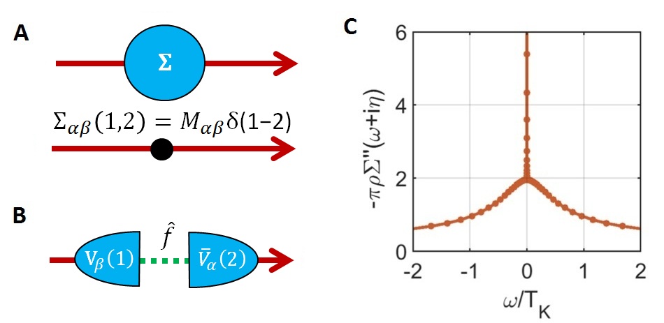
Figure 2: (A) In a conventional broken symmetry state, the coarse-grained electronic self-energy (top) is instantaneous and local. (B) Order fractionalization leads to a factorization of the self-energy into two spinorial components, linked by a low energy fermionic bound-state (bottom). (C) The irreducible self-energy in the single-channel single-impurity Kondo model, computed using NRG, displaying a sharp fermionic pole, on top of a Fermi liquid background (see supplementary material B).

Fig. 2C shows the result of a NRG calculation of the one-particle irreducible electron self-energy in the spin-1/2 Kondo model, indicating that it contains a sharp, resolution-limited pole at zero energy, with the asymptotic form $\Sigma_{\alpha\beta}\sim\delta_{\alpha\beta}\bar{V}V/\omega$. The pole demonstrates the development of a many-body fermionic bound-state at the Fermi energy carrying $S=1/2$ and charge $e$; the sharpness of the pole confirms that the spectral decomposition of the emergent f-electron field has no overlap with one-particle excitations of the conduction sea, i.e it is an emergent fermion, described by the Lagrangian ${\cal L}_{f}=f^{\dagger}_{\sigma}(-i\partial_{t})f_{\sigma}$. The background to the peak can be fit with $\omega^{2}$ at low energies and is due to Fermi-liquid interactions (c.f. Supplementary Materials B).

To confirm that the local moment fractionalizes into a pair of fermions, we apply a small external magnetic field, under which the Lagrangian acquires a term proportional to the magnetization $\vec{M}=\frac{1}{2}\psi^{\dagger}\vec{\sigma}\psi+\vec{S}$, i.e. ${\cal L}\rightarrow{\cal L}-\vec{B}.\vec{M}$. Equivalently, we can employ a Gallilean transformation into a reference frame rotating with angular velocity $\vec{\omega}=\left({g\mu_{B}}\right)\vec{B}$. In the rotating reference frame, $\psi\rightarrow U\psi$ and $f\rightarrow Uf$ where $U=e^{-it\vec{\omega}\cdot\vec{\sigma}/2}$, and under this transformation,

$${\cal L}_{f}\rightarrow f^{\dagger}\left(-i\partial_{t}-\vec{\omega}\cdot{\vec{\sigma}}/{2}\right)f={\cal L}_{f}-(g\mu_{B})\vec{B}\cdot\vec{S}_{f}$$ (3)

where $\vec{S}_{f}\equiv f^{\dagger}_{\alpha}\left(\frac{\vec{\sigma}}{2}\right)_{\alpha\beta}f_{\beta}$. Comparing this to the original $\vec{M}$, we can identify $\vec{S}_{f}$ as the spin, fractionalized into a product of Dirac (i.e. complex) fermions.

Traditional treatments of the single channel Kondo model describe the low energy physics in terms the formation of a Kondo singlet between an electron and local moment, that develops as the Kondo coupling $J$ scales to infinitely strong coupling; the expulsion of the electrons from the site of the Kondo singlet gives rise to unitary scattering, and the development of a local Fermi liquid Nozières and Blandin (1980). To understand how the traditional viewpoint is consistent with fractionalization we have analytically calculated the electron self-energy in the strong coupling limit of large $J$, using the Lehmann representation of the electron Green’s function in terms of the exact eigenvalues. Remarkably, as in the NRG calculation, the self-energy $\Sigma(\omega)=(3J/2)^{2}/{\omega}$ contains a single pole (Supplementary material D). Whereas we might have expected a large static self-energy of order $\Sigma\sim-J$, corresponding to the binding of the electron into the singlet, instead the Kondo scattering off the singlet is dynamical. As in the NRG calculation, we are forced to interpret the zero-energy pole in the self-energy as the fractionalization of the local moment into a fermion, hybridized with the conduction sea to form a local Fermi liquid, as summarized in Fig. 1A. Once we acknowledge that scattering off the Kondo singlet is dynamical at the strong-coupling fixed point, we are able to reconcile fractionalization with the traditional view of the Kondo effect.

An important aspect of fractionalization is the emergence of an internal gauge symmetry. The established view is that fractionalized excitations carry an internal gauge charge Senthil and Fisher (2000); Senthil et al. (2004); Hansson et al. (2004); Vishwanath et al. (2004); Senthil et al. (2005); Fradkin and Shenker (1979). The fractionalized spin is invariant under gauge transformations of the emergent f-excitations, $f_{\alpha}\rightarrow e^{i\theta(t)}f_{\alpha}$. Moreover the composite fermion $(\vec{\sigma}\cdot\vec{S})\psi$ involves a product of the hybridization and the f-electron, $\bar{V}f_{\sigma}$ that is invariant under $U(1)$ transformations of both fields $f_{\sigma}\rightarrow e^{i\theta(t)}f_{\sigma}$, $V\rightarrow e^{i\theta(t)}V$. When these transformed fields are substituted into the action, it becomes ${\cal L}_{f}\rightarrow f^{\dagger}(i\partial_{t}+A_{0})f$, where $A_{0}=\dot{\theta}$ is an emergent gauge field coupled to the number operator of the f-electrons. The path-integral approaches suggest that the right action for the f-electrons contains an additional topological term that controls the irreducible representation of the spin of the form ${\cal L}_{f}=f^{\dagger}i\partial_{t}f+A_{0}(n_{f}-Q)$ where $Q=1$ for the $SU(2)$ Kondo model. With this formulation we can always choose a gauge where $V(t)$ is real and the phase fluctuations are entirely absorbed into $A_{0}(t)$. The NRG results suggest that the mean-field saddle point describing a fractionalized ground-state in which $A_{0}=0$ captures the essential physics of the excitations of the $S=1/2$ SU(2) Kondo model. Fourier transforming the conduction electron self-energy into the time-domain, we see it exhibits long-range temporal correlations

$$\Sigma(t_{1}-t_{2})\xrightarrow{|t_{1}-t_{2}|\rightarrow\infty}|V|^{2}\hbox{sgn}(t_{1}-t_{2})/2.$$ (4)

In the single-channel Kondo model these correlations do not break any physical symmetry but they will be important for our subsequent discussion.

Induced Order Fractionalization. To address our original question regarding order fractionalization, we next turn to the two-channel Kondo (2CK) model where the channels of screening electrons are indexed by $\lambda=1,2$. The channel-symmetric two channel Kondo model has a quantum critical ground-state Andrei and Destri (1984); Tsvelick and Wiegmann (1984); Affleck and Ludwig (1993) , which can be loosely interpreted as a resonant-valence-bond (RVB) state of singlet between the spin and each of the two conduction channels (Fig. 3A). As we now show, breaking this channel symmetry induces order fractionalization. The 2CK exchange interaction is

$$H_{I}=J\psi^{\dagger}_{\lambda}(\vec{\sigma}\cdot\vec{S})\psi_{\lambda}+\delta J\hat{\cal O},$$ (5)

where the channel asymmetry $\delta J$ couples to the composite operator $\hat{\cal O}=(\psi^{\dagger}_{1}\vec{\sigma}\psi_{1}-\psi^{\dagger}_{2}\vec{\sigma}\psi_{2})\cdot\vec{S}$, inducing an asymmetric Kondo coupling $J\pm\delta J$ in the two channels. $\delta J$ plays the role of an external field that induces composite order $\langle{\cal O}\rangle$. Renormalization group studies tell us that a finite channel asymmetry $\delta J>0$ destabilizes the quantum critical point, stabilizing a Kondo singlet in the strongest channel Nozières and Blandin (1980), here associated with the $\lambda=1$, loosely interpreted as a valence bond solid (VBS) state (Fig. 3B). As in the one-channel Kondo model, this implies the formation of a fermionic bound-state

$$J(\vec{\sigma}_{\alpha\beta}\cdot\contraction{}{\vec{S}}{)}{\psi}\vec{S})\psi_{\lambda\beta}=\bar{V}_{\lambda}\hat{f}_{\alpha},\qquad(\lambda=1,2),$$ (6)

but with a channel-dependent amplitude $\bar{V}_{\lambda}=(\bar{V},0)$ that projects into the strongest channel. The quantum numbers of the composite fermion divide into two: a c-number spinor $\bar{V}_{\lambda}$ that carries the channel quantum number and a residual fermion with spin and charge but no channel index.

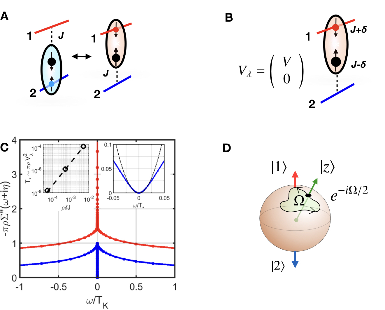
Figure 3: (A) The symmetric two-channel Kondo model forms a quantum critical state where the Kondo singlets are delocalized between channels. (B) Application of channel asymmetry stabilizes a Kondo singlet on one channel, defined by a spinor order parameter. (C) A fermionic pole is induced in the strongest channel, indicating the presence of a selective hybridization $\bar{V}_{\lambda}=(V,0)$ between the fractionalized moment and the two screening channels. The red curve is shifted by 0.5 unit vertically upward for clarity. (Insets) left: $T_{*}$ vs $\rho\delta J$. right: the low-frequency regime of self-energy in channel 2 vs. $\omega$ showing Fermi liquid behavior (dashed black line is an $\omega^{2}$ fit). (D) Adiabatic rotation of the channel asymmetry along a path subtending a solid angle $\Omega$ leads between channels leads to an $e^{-i\Omega/2}$ Berry phase, reflecting the half-integer nature of the induced order.

Fig. 3C displays the self-energy of a channel-asymmetric spin-$1/2$ 2CK model, calculated using NRG. For $\delta J>0$, a sharp, resolution-limited quasiparticle pole forms in the strongest $\lambda=1$ channel, leading to a pole in the self-energy, $\Sigma_{\lambda\lambda^{\prime}}\sim\bar{V}_{\lambda}V_{\lambda^{\prime}}/\omega$. The product form of the self-energy follows from the projection into the strongest channel. By Fourier transforming this result, we confirm that at long times, the self-energy factorizes

$$\Sigma_{\lambda\lambda^{\prime}}(t_{2}-t_{1})\xrightarrow{|t_{2}-t_{1}|\rightarrow\infty}\bar{V}_{\lambda}(t_{2})V_{\lambda^{\prime}}(t_{1}){\rm sgn}(t_{2}-t_{1})/2.$$ (7)

This factorization into two spinors means that the singular part of the self-energy does not transform under an irreducible representation, but instead as a reducible sum of a vector and scalar representation, i.e $1/2\otimes 1/2=0+1$. If we are to preserve Landau’s notion that order parameters transform under irreducible representations, then we are forced to acknowledge that the spinor $V_{\lambda}$ is the relevant order parameter and we have order fractionalization.

A way of exposing the spinorial character of the order is to adiabatically rotate the spinor $V_{\lambda}$ by slowly rotating the channel asymmetry, which we may write $\delta J(\hat{n}(t)\cdot\vec{{\cal O}})$, where $\vec{{\cal O}}=\psi^{\dagger}_{\lambda}\vec{\alpha}_{\lambda\lambda^{\prime}}(\vec{\sigma}\cdot\vec{S})\psi_{\lambda^{\prime}}$ is the composite “channel magnetization”, defined in terms of three Pauli matrices $\vec{\alpha}=(\alpha_{1},\alpha_{2},\alpha_{3})$, and $\hat{n}(t)$ is the asymmetry field. In this adiabatic evolution of the Kondo singlet, the channel selective hybridization is then determined by $(\vec{\alpha}_{\lambda\lambda^{\prime}}\cdot\hat{n})V_{\lambda^{\prime}}=+V_{\lambda}$. By slowly varying $\hat{n}(t)$ along a closed path, we can characterize the topology of the order parameter by examining the corresponding Berry phase factor $e^{-i\gamma}=e^{-i\Omega S}$ where $\Omega$ is the solid angle enclosed by the path and $S$ determines the spin of the order parameter (Fig. 3D). To calculate $\gamma$ we go to the extreme strong coupling limit, where $\delta J\gg\Lambda$, the electron band-width. In this limit the channel Kondo singlet becomes entirely local, taking the form $\left|z\right\rangle=\sum_{\lambda=1,2}z_{\lambda}|\lambda_{s}\rangle$, where $z=(z_{1},z_{2})\equiv V_{\lambda}/|V|$ is a unit spinor and $|\lambda_{s}\rangle=\frac{1}{\sqrt{2}}\left(|\lambda\uparrow,\Downarrow\rangle-|\lambda\downarrow,\Uparrow\rangle\right)$ denotes a singlet formed between the local moment ($\Uparrow$) and electron ($|\lambda\uparrow\rangle$) in channel $\lambda$. When $\hat{n}(t)$ is rotated through a solid angle $\Omega$, the spinor $z_{\lambda}(t)$ evolves adiabatically, and the ground-state wavefunction acquires a Berry phase given by $\gamma=-i\oint dt(z^{\dagger}\partial_{t}z)=\frac{1}{2}\Omega$ (cf. Supplementary Material C). The factor of $1/2$ confirms the half-integer channel spin of the state.

We also note the application of the symmetry-breaking field $\delta J$ induces an expectation value of the composite order parameter $\langle\vec{{\cal O}}\rangle\propto V^{*}_{\lambda}\vec{\alpha}_{\lambda\lambda^{\prime}}V_{\lambda^{\prime}}$, indicating that the induced composite order has fractionalized into a product of channel hybridization spinors. From this exercise, we see that order fractionalization (OF) is manifested in three separate ways: (i) a splitting of the composite fermion into a spinor boson and a fermion; (ii) a fractionalization of the local moment into a product of fermion excitations and (iii) fractionalization of the composite order parameter into a product of spinorial order parameters.

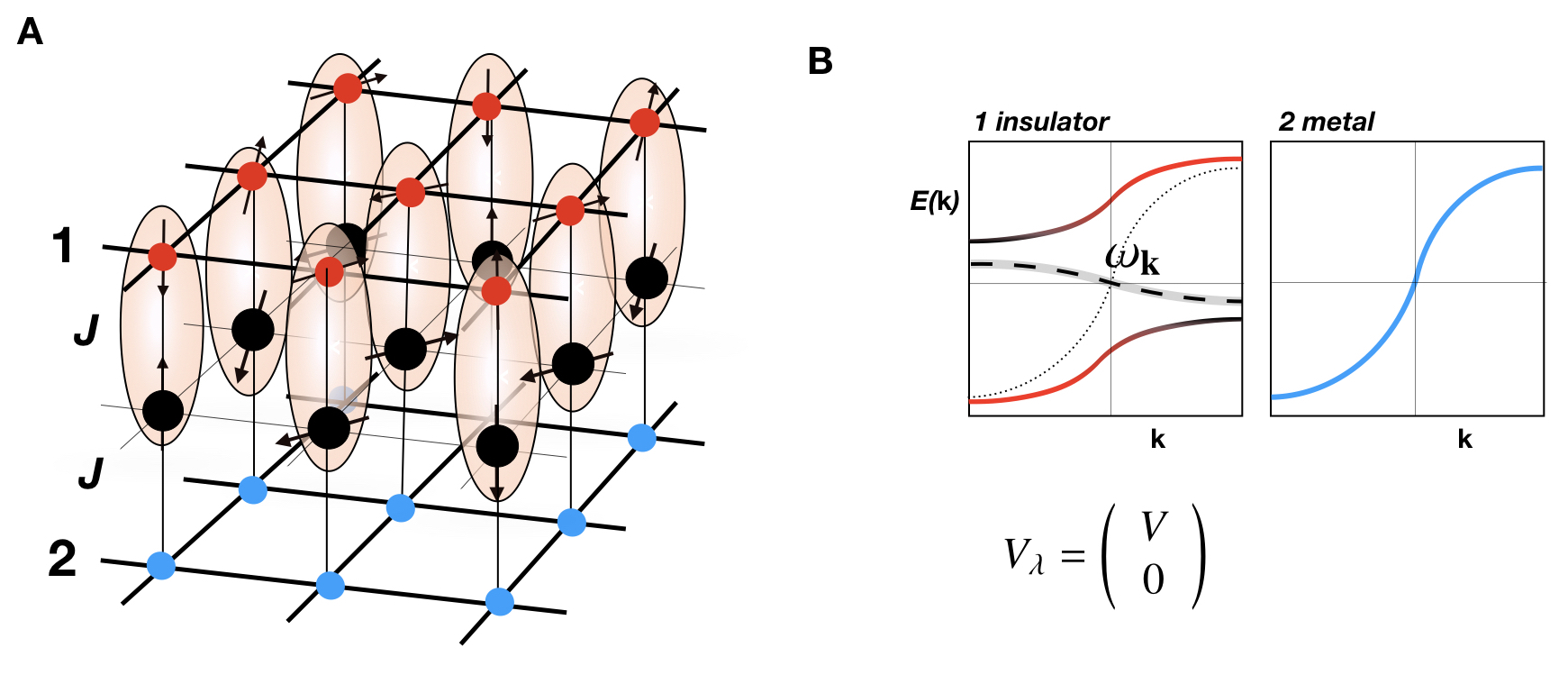
Figure 4: (A) In a 2CK lattice model at $d=2,3$ dimensions we expect order fractionalization to lead to spontaneous channel symmetry breaking, forming Kondo singlets in one channel, with a channel-spinor defining the selective hybridization of the fractionalized local moments. (B) The channel spinor leads to a Kondo insulator in the hybridized channel (1) with a hybridization gap. The dashed line indicates the dispersion $\omega_{{\bf{k}}}$ of the emergent f-electron. Channel 2 remains a gapless insulator.

Spontaneous Order Fractionalization. Induced order fractionalization in the two-channel Kondo impurity model enables us to conjecture spontaneous order fractionalization in lattice models. The key idea is that order fractionalization at one site produces a channel-symmetry breaking Weiss field at its neighbors. This then provides positive feedback that allows a fractionalized ordered state to develop spontaneously due to the fragile nature of the critical system. The NRG results confirm that the path integral gauge theory approach provides a qualitatively correct description of the fractionalization at a mean-field level, which can then be used to describe spontaneous order fractionalization in a Kondo lattice. As in conventional mean-field theories, the Gaussian order parameter fluctuations about such a mean-field theory are finite in dimensions $d\geq 2$, allowing a stable spontaneous order fractionalization Wugalter et al. (2018); Zhang et al. (2018). Thus in the two-channel Kondo lattice at half filling, spontaneous OF means that the system behaves as a Kondo insulator in one channel, remaining metallic in the other. With this reasoning, symmetry-breaking phases of this type characterized in dynamical mean-field theory calculations Jarrell et al. (1996); Nourafkan and Nafari (2008); Hoshino et al. (2011) can be interpreted as order-fractionalized phases.

Patterns of Fractionalization. In our studies we have highlighted just one example of how broken channel symmetry induces an order fractionalization. By varying the asymmetry field ${\cal O}$ we can classify family of fractionalized order, which we have summarized in Table 1. Class (a) is fractionalization of the single channel Kondo model, with no broken symmetry. Class (a’) is discussed below. Our NRG calculation gives us a channel FM, listed as class (b). To obtain the other patterns of fractionalization, we we have emplyed two different strategies. The first is to take advantage of the high symmetry of the 2CK to rotate the pattern of fractionalization. In the 2CK the two channel symmetry and particle-hole symmetries form part of single SO(5) symmetry Affleck et al. (1992); Zhang (1997); Hoshino and Kuramoto (2015) (see supplementary material E). This allows us to rotate the asymmetry field $\vec{{\cal O}}=({\cal O}_{1},\dots\cal O_{5})$ within a five dimensional space, in which the first three components correspond to channel magnetization as discussed above, while the fourth and fifth correspond to a composite pair operator ${\cal O}_{4}-i{\cal O}_{5}\equiv\psi_{1}\vec{\sigma}i\sigma_{2}\psi_{2}\cdot\vec{S}$. When we rotate the asymmetry field from a channel magnet into a composite pair, we can follow the corresponding transformation in the composite fermion, showing that it acquires a Boguilubov structure as shown in class (c). Finally, we can obtain a fifth class (d) by reversing the roles the roles of channel and spin to obtain a quadrupolar Kondo model. Here the fractionalized excitations carry the channel index $\bigl{[}(\vec{S}\cdot\vec{\sigma})\psi\bigr{]}_{\lambda\alpha}\to V_{\alpha}f_{\lambda}$ while the order parameter $V_{\alpha}$ is a spinor that breaks time reversal symmetry.

Each of the examples of order fractionalizalization apply to two-channel Kondo models. We can employ a second strategy to examine order fractionalization in one channel Kondo systems, by using a reformulation of the 2CK in terms of Majorana fermions in which the spin-density of the two channels is replaced by the spin and isospin density of a “compactified” two-channel Kondo model, $(\psi^{\dagger}_{1}\vec{\sigma}\psi_{1},\psi^{\dagger}_{2}\vec{\sigma}\psi_{2})\rightarrow(\psi^{\dagger}\vec{\sigma}\psi,\tilde{\psi}^{\dagger}\vec{\tau}\tilde{\psi})$ Coleman et al. (1995) where $\tilde{\psi}$ is a Nambu spinor. In this form, the fractionalization can analyzed (see supplementary materials D) by studying the family of Kondo interactions $J\tilde{\psi}(\vec{\sigma}+(1-\epsilon)\vec{\tau})\tilde{\psi}\cdot\vec{S}$, where $\epsilon\neq 0$ breaks the channel symmetry. This formulation can be examined in the strong coupling limit, demonstrating that the local moment fractionalizes into Majorana, rather than Dirac fermions Coleman et al. (1994); Xu and Sachdev (2010), as shown in entry a’ of Table 1.

Kondo Model	3 body state	Class	Composite Fermion	Induced Order	Asymmetry ${\cal O}$	OF
One Channel	$(\vec{\sigma}\cdot\contraction{}{\vec{S}}{)_{\alpha\beta}}{\psi}\vec{S})_{\alpha\beta}\psi_{\beta}$	a	${V}\ f_{\beta}$	(Fermi Liquid)	—	—
		a’	$(\vec{\sigma}\cdot\vec{\eta})_{\alpha\beta}{\cal V}_{\beta}$	Odd $\omega$ pairing	$\psi_{\uparrow}\psi_{\downarrow}S^{+}+{\rm H.c}$	${\cal V}_{\uparrow}{\cal V}_{\downarrow}+{\rm H.c}$
			Abrahams et al. (1995); Coleman et al. (1994)
Two channel	Spin	b	$V_{\lambda}f_{\alpha}$	Channel FM	$\psi_{\lambda}^{\dagger}(\vec{\sigma}\cdot\vec{S})\psi_{\lambda^{\prime}}$	$\bar{V}_{\lambda}V_{\lambda^{\prime}}$
	$(\vec{\sigma}\cdot\contraction{}{\vec{S}}{)_{\alpha\beta}}{\psi}\vec{S})_{\alpha\beta}\psi_{\lambda\beta}$		Hoshino et al. (2011); John S. Van Dyke (2018)
		c	$V_{\lambda}f_{\alpha}+\Delta_{\lambda}\tilde{\alpha}f^{\dagger}_{-\alpha}$	Composite pairing	$\psi_{1}(\vec{\sigma}\cdot\vec{S})\sigma_{2}\psi_{2}$	$V_{1}\Delta_{2}-V_{2}\Delta_{1}$
				Emery and Kivelson (1992); Coleman et al. (1999)
	Quadrupolar
	$(\vec{\gamma}\cdot\contraction{}{\vec{S}}{)_{\lambda\lambda^{\prime}}}{\psi}\vec{S})_{\lambda\lambda^{\prime}}\psi_{\lambda^{\prime}\alpha}$	d	$V_{\alpha}f_{\lambda}$	Hastatic Order	$\psi_{\alpha}^{\dagger}\vec{\sigma}(\vec{\gamma}\cdot\vec{S})\psi_{\beta}$	$\bar{V}_{\alpha}V_{\beta}$
				Chandra et al. (2013)

Table 1: Classifying different patterns of fractionalization in single-channel and two-channel Kondo systems, obtained by adding asymmetry fields to one and two-channel Kondo models. In class a’ $\vec{\eta}=(\eta_{1},\eta_{2},\eta_{3})$ denotes a vector of three emergent Majorana fermions that fractionalize the local moment spin, $\vec{S}\equiv\frac{i}{2}\vec{\eta}\times\vec{\eta})$ Coleman et al. (1994). Class b channel rotations of the asymmetry field $\cal O$, whereas class c are obtained from an SO(5) rotation of the channel asymmetry (Supplementary Material XXX). In class c $\tilde{\alpha}$ denotes $\tilde{\alpha}\equiv{\rm sign}{\alpha}$.

Candidate materials with composite order corresponding to these different fractionalization patterns have been proposed in the context of heavy fermion materials. materials. The SO(5) rotations of the channel FM into a composite ordered state Coleman et al. (1999) (Table 1, class c) has been proposed for the heavy fermion superconductor NpPd₂Al₅ Flint et al. (2008). An example of class (d) is the “hastatic” hidden order proposed for phases of URu₂Si₂ Chandra et al. (2013) and PrTi₂Al₂₀ John S. Van Dyke (2018). The Majorana fractionalization class (a’) has been recently proposed as a candidate for the strange insulating state in SmB₆ Erten et al. (2017). Each of these materials are candidates for the realization of spontaneous order fractionalization.

Order Fractionalization Conjecture. We can also envisage spontaneous order fractionalization in broader contexts beyond Kondo lattices; for example in the Hubbard model where the combination of spin and fermion is now replaced by a three fermion bound-state. This leads us to conjecture that in this more general situation, the OF will involve a fractionalization of a three-fermion bound-state into two components: a bosonic “corona ” surrounding a “dark fermion” located at the center-of-mass. This process has the effect of partitioning the quantum numbers $\Lambda=(\{\lambda\},\{\alpha\})$ of three-body composite, into two parts, the $\lambda$ variables reside exclusively in the bosonic corona, while the $\alpha$ variables reside in the dark fermion. The order fractionalization conjectured (OFC) for this general case takes the form

$$\bigl{(}\mathrel{\mathop{{\psi\psi\psi}}^{\displaystyle\raise-0.7pt\hbox{$\scriptscriptstyle|$}\mathrel{\mkern-9.0mu}\mathrel{{\bf\smash{{\phantom{-}\above 1.0pt\phantom{-}}}}}\mathrel{\mkern-9.0mu}\raise-0.7pt\hbox{$\scriptscriptstyle|$}\mathrel{\mkern-9.0mu}\mathrel{{\bf\smash{{\phantom{-}\above 1.0pt\phantom{-}}}}}\mathrel{\mkern-9.0mu}\raise-0.7pt\hbox{$\scriptscriptstyle|$}}}\bigr{)}_{\Lambda}(x)=V^{\lambda}_{\alpha\alpha^{\prime}}(x)f_{\alpha^{\prime}}(x).$$ (8)

Here $(\psi\psi\psi)_{\Lambda}(x)$ corresponds to a combination of creation or annihilation operators with center of mass $x$, that transform under fundamental representations of the $\Lambda$. $V^{\lambda}_{\alpha\alpha^{\prime}}(x)$ and $f_{\alpha}(x)$ are the order parameter corona and the dark fermion respectively. In the simplest cases, $V^{\lambda}_{\alpha\beta}=V^{\lambda}\delta_{\alpha\beta}$ is diagonal, and the corona and dark fermion share a common $U(1)$ gauge symmetry. The general matrix structure of the order fractionalization allows for a non-abelian partition of the quantum numbers, with an internal SU(N) gauge symmetry associated with the quantum numbers $\alpha$. This more general form is required to understand the example of composite pairing shown in Table. 1.

The OFC also implies that the corresponding self-energy factorizes as follows

$$\Sigma_{\Lambda\Lambda^{\prime}}(2,1)\xrightarrow{|2-1|\rightarrow\infty}\bar{V}_{\lambda}(2)g(2-1)V_{\lambda^{\prime}}(1).$$ (9)

where $g(2-1)$ is the one-particle propagator of the dark fermion. In a lattice, the dark fermions will generically delocalize with dispersion $\omega_{{\bf{k}}}$, forming a Fermi surface ${\bf k}\in\{{\bf{k}}_{F}^{*}\}$ where $\omega_{{\bf{k}}_{F}^{*}}=0$ vanishes. In space time, the asymptotic Green’s function of the dark Fermions,

$$g(\vec{x},t)\sim\delta_{\alpha\alpha^{\prime}}\frac{e^{i\vec{k}_{F}^{*}\cdot\vec{x}}}{x-v_{F}(\hat{x})t},$$ (10)

where $\vec{k}_{F}^{*}(\hat{x})={{\bf{k}}}_{F}^{*}$ is the Fermi wavevector at the extremal point on the Fermi surface where the group velocity $\vec{v}_{F}=v_{F}\hat{x}$ is parallel to $\vec{x}$. This defines a kind of “light cone” on which $g$ is arbitrarily large. The factorization of the self-energy into a product of spinors is the conjectured outcome of order fractionalization in a fermionic system, and constitutes a generalization of the concept of off-diagonal long range order into the time domain. We also note that the singularity $\Sigma_{\lambda,\lambda^{\prime}}(\omega,{\bf{k}}_{F}^{*})\sim\bar{V}_{\lambda}V_{\lambda^{\prime}}/(\omega-\omega_{{\bf{k}}})$ in the self-energy at the dark Fermi surface leading to zeroes in the electronic Green’s function $G(\omega,{\bf{k}}_{F}^{*})=0$ Stanescu et al. (2007); Seki and Yunoki (2017). There is an interesting possible link with singularities in the electron self-energy observed in cluster dynamical mean-field studies of the Hubbard model Sakai et al. (2016) and also proposed as a phenomenological explanation of Fermi arcs in under-doped cuprate superconductors Yang et al. (2006); Konik et al. (2006).

Conventional and fractionalized order can be delineated in various ways. There are a number of quantum materials, including NpPd₅Al₂, CeCoIn₅, UBe₁₃, PrV₂Al₂₀ and PrTi₂Al₂₀ where spin or quadrupolar Kondo effects coincide with phase transitions into broken symmetry states. An important “fingerprint” of fractionalization is the appearance of dark fermionic bound-states, that may be detected using spectroscopies such as angle resolved photoemission (ARPES) or scanning tunneling microscopy (STM). For example if in CeCoIn₅ the Kondo effect coincides with the development of superconductivity, then STM should detect an expansion of the Fermi surface at the superconducting transition; in neutral cases the thermal conductivity would be an ideal probe for this Fermi surface change.

An intriguing question is whether the different topologies of fractionalized order can be detected experimentally. For example in UBe₁₃ and Pr (V,Ti)₂Al₂₀ where the channel index is spin, it may be possible to externally manipulate the channel-symmetry breaking Kondo-effect: rotating the order spatially through 360^∘ to create a $\pi$ phase shift may be detected in a channel interferometer; rotating the order in time using optical methods may lead to a breathing Fermi surface which might be measured using a channel-selective conductivity.

We end by noting that despite the spin-statistics theorem, relativistic versions of order fractionalization are possible since Lorentz invariance does not prohibit bosons that carry half-integer isospin. A classic example is the Higgs boson, a spinor which carries half-integer weak isospin and could conceivably emerge as a fractionalized order parameter of more fundamental Fermi fields.

In conclusion we have presented a mechanism for the fractionalization of order parameters through the formation of fermionic poles in the self-energy; this enables long-time factorization of the self-energy into products of order parameters transforming under the fundamental representation of the symmetry group. We have provided crucial substantiating examples in the single and two-channel impurity Kondo models. These results have led us to conjecture that such phenomena may appear spontaneously in a lattice as suggested by several experimental, mean-field and computational results.

We would like to thank C. Batista, M. Civelli, R. Flint, E. König, M. Imada, M. Oshikawa, P. Phillips, A. Rosch, S. Thomas, S. Sondhi, S. Sachdev, T. Senthil and A. Wugalter for stimulating discussions. The conceptual beginnings of this work were supported by NSF grant DMR-1309929 (P. Coleman). Yashar Komijani is supported by a Center for Material Theory postdoctoral Fellowship. We thank Princeton University, Princeton USA (P. Chandra) the Flatiron Institute, New York USA (Y. Komijani and P. Coleman) and the Institute for Solid State Physics, Kashiwanoha, Japan (P. Chandra and P. Coleman) for their hospitality during the later writing stages of this manuscript.

Supplementary Material

This supplementary material contains additional details and proofs for key statements in the paper. Section A contains details of the Numerical Renormalization Group (NRG) calculation. Section B contains a derivation of the fermionic pole in the self-energy of the Kondo problem using Fermi-liquid theory, in the single-channel and channel-asymmetric two-channel Kondo models. Section C contains a proof of the Berry phase accumulated by the ground state under an adiabatic time-evolution, establishing the spinorial character of the order parameter. Section D shows that the projective form of the self-energy and the fractionalization pattern can be directly extracted by studying the the strong coupling limit of single-channel Kondo problem for both usual and the compactified model. In section D we review the SO(5)$\times$SU(2) symmetry group of the two-channel Kondo problem and use the extended symmetry to study various patterns of fractionalization.

Contents

1. .1 Details of the NRG calculations
2. .2 Fermionic pole in the Kondo self energy: relationship to Fermi-liquid theory
3. .3 Berry phase calculation
4. .4 Strong Coupling analysis of the single-channel Kondo Model
   1. .4.1 Fractionalization in the strong coupling limit of single-channel Kondo model
   2. .4.2 Majorana Fractionalization
5. .5 Analysis of SO(5) symmetry breaking in the two-channel Kondo model
   1. .5.1 SP(4) symmetry of the two-channel Kondo problem
   2. .5.2 The projective form of the self-energy
   3. .5.3 Fractionalization pattern and composite ordering

.1 Details of the NRG calculations

NRG calculations were performed using the density-matrix NRG code Tóth et al. (2008); Tóth and Zaránd (2008) with a flat density of states, which produces the imaginary part of the local Green’s functions (e.g. $G(z)=\langle\langle\psi_{\sigma};\psi_{\sigma}^{\dagger}\rangle\rangle_{z}$) at discrete frequencies determined by the Wilson discretization as follows

$$-G^{\prime\prime}(\omega+i\eta)=\frac{1}{Z}\sum_{n,m}|\left\langle m|\psi_{\sigma}^{\dagger}|n\right\rangle|^{2}\pi\delta(\omega+E_{n}-E_{m})(e^{-\beta E_{m}}+e^{-\beta E_{n}}),$$ (11)

where $\left|m\right\rangle$ and $\left|n\right\rangle$ are many-body eigenstates with energies $E_{m}$ and $E_{n}$, respectively, and $Z=\sum_{n}e^{-\beta E_{n}}$ is the partition function. Our methodology takes account of the SU_charge(2)$\times$SU_spin(2) and SU_spin(2)$\times$SU_charge1(2)$\times$SU_charge2(2) symmetries of the one and the two-channel models, respectively to simplify calculation of the matrix elements. The calculations employed 500 multiplets and a Wilson parameter $\Lambda=1.8$, with a Wilson chain length $L=80$. The full-density matrix calculation ensures that the discrete results (11) satisfy the sum-rules enforced by the commutation relations. The code uses an interpolative log-Gaussian broadening, with the Kernel defined as follows Bulla et al. (2001); Tóth et al. (2008)

$$K_{int}(\omega,\omega_{i}) = \frac{1}{b\sqrt{\pi}}e^{-[x(\omega)-x(\omega_{i})]^{2}/b^{2}}\frac{dx}{d\omega_{i}},$$ (12)

$$x(\omega) = \frac{1}{2}\tanh({\omega}/{T_{Q}})\log[(\omega/T_{Q})^{2}+e^{\eta}]$$ (13)

where the ‘quantum temperature’ $T_{Q}$ is chosen to be $10^{-15}$ and $\eta\approx T_{Q}$ for our zero temperature calculations. We have taken the logarithmic broadening parameter $b$ to be $b=0.6$. This leads to

$$-G^{\prime\prime}(\omega+i\eta)=\frac{1}{Z}\sum_{n,m}|\left\langle m|\psi_{\sigma}^{\dagger}|n\right\rangle|^{2}\pi K(\omega,E_{m}-E_{n})(e^{-\beta E_{m}}+e^{-\beta E_{n}}).$$ (14)

The normalization

$$\int{d\omega}K_{int}(\omega,\omega_{i})=1$$ (15)

ensures that the sum-rules are satisfied. Following the standard approach, the Hilbert transform is applied to the broadened data to obtain both real and imaginary parts of the Green’s function.

We compute the irreducible self-energy for the Kondo problem from the conduction electron Green’s function $G(z)$. In principle, the self-energy can be calculated directly from the relation

$$\Sigma(z)=g^{-1}(z)-G^{-1}(z)$$ (16)

where $g(z)$ is the bare conduction electron propagator in the absence of the impurity ($J=0$). However, at the Fermi energy $G^{-1}(z)$ is singular and so this expression requires careful regularization.

In practice, we found it easier to divide the calculation into two parts. First we calculated the electron T-matrix $T(z)$, defined by the relation

$$G(z)=g(z)+g(z)T(z)g(z)$$ (17)

from which we obtain

$$T(z)=\frac{G(z)-g(z)}{g(z)^{2}}.$$ (18)

The regularized self- energy was then calculated from the T-matrix, using the relationship

$$\Sigma(z)=\lim_{\epsilon\to 0}\hphantom{A}\frac{T(z)}{1+(1-\epsilon)g(z)T(z)},\qquad g(z)=\langle\langle\psi^{\vphantom{\dagger}}_{\sigma};\psi^{\dagger}_{\sigma}\rangle\rangle_{z}\Big{|}_{J=0}.$$ (19)

This limiting procedure was used to ensure that the $\Sigma(z)$ has the correct analytical properties. A finite $\epsilon$ leads to some residual broadening of the peak. In our calculations, we used $\epsilon=10^{-8}$.

.2 Fermionic pole in the Kondo self energy: relationship to Fermi-liquid theory

We can gain analytic insight into our results using Fermi-liquid theory. From Fermi-liquid theory Affleck and Ludwig (1993); Shi and Komijani (2017) we know that the phase shifted quasi-particles have a Fermi-liquid interaction with a single scale: the Kondo temperature. This gives rise to a low energy scattering $T$-matrix of the form

$$-\pi\rho T(\omega+i\eta)=i-\frac{\omega}{T^{\prime}_{K}}-i\zeta\frac{\omega^{2}}{T_{K}^{\prime 2}}+O(\omega^{3}),$$ (20)

where $T^{\prime}_{K}$ is proportional to the weak-coupling Kondo temperature $T_{K}\sim D\sqrt{J\rho}e^{-1/\rho J}$. Inserting this expression, together with a flat density of states $g(\omega+i\eta)=-i\pi\rho$ into (18), the corresponding irreducible self-energy is then

$$\pi\rho\Sigma(\omega+i\eta)=\Big{[}{\frac{1}{\pi\rho T(\omega+i\eta)}-i}\Big{]}^{-1}=\frac{T^{\prime}_{K}}{\omega+i(\zeta-1)\omega^{2}/T^{\prime}_{K}+i\eta}.$$ (21)

This result is plotted in Fig. 5. The background beneath the delta-function pole is thus understood as a result of the $\omega^{2}$ Fermi liquid scattering rate.

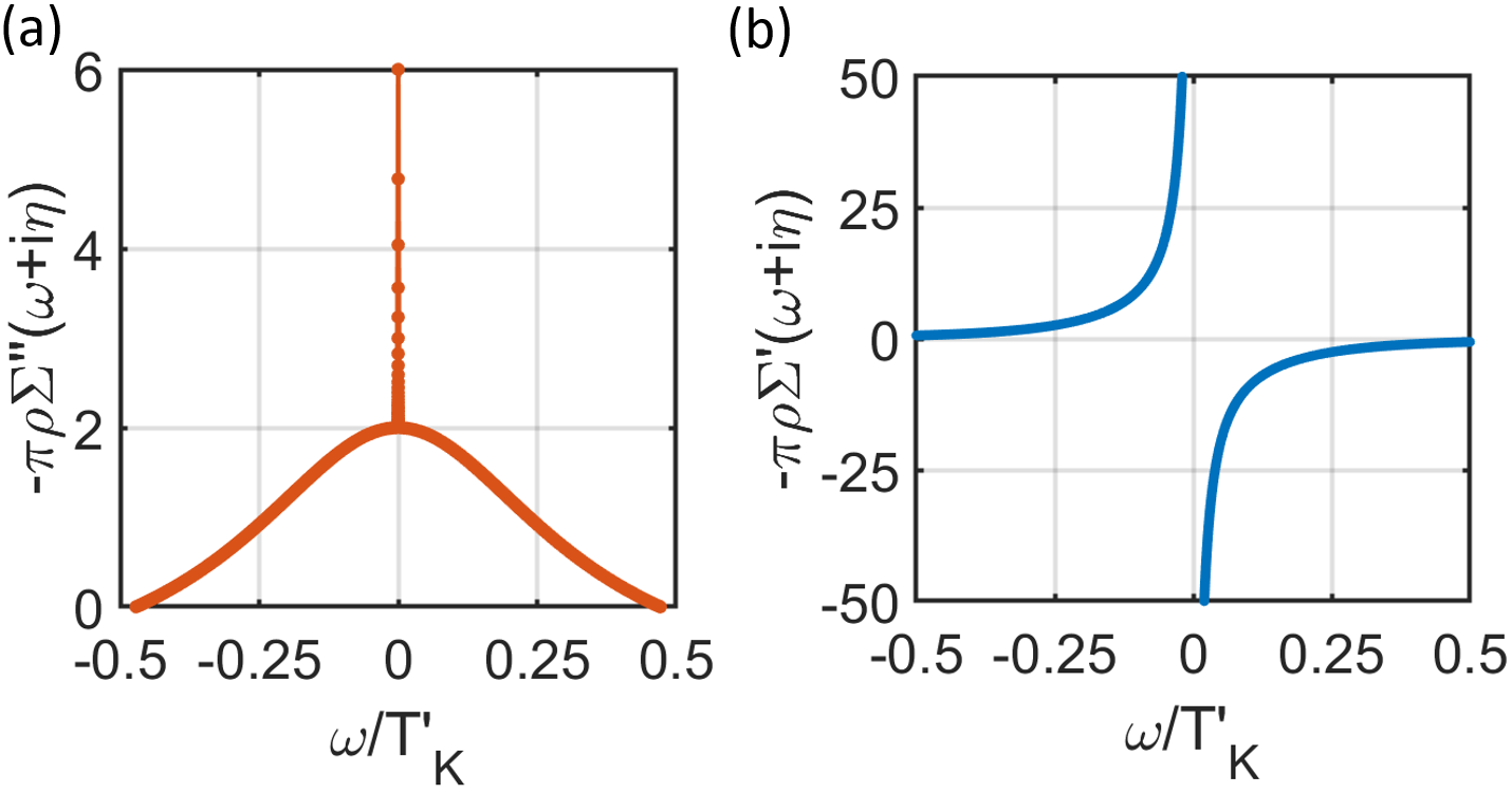
Figure 5: (a) The imaginary part of the irreducible self-energy extracted from Fermi-liquid theory. The background is a result of the inelastic scattering of the composite quasiparticle at finite energy as shown in Eq. (20). (b) The real part shows the $1/\omega$ signature of long-range order in time.

The parameter $\zeta$ determines the value of background offset $-\pi\Sigma^{\prime\prime}(\omega\to 0)=\zeta-1$, and does not affect any qualitative features of the discussion. In order to recover our numerical results $-\pi\Sigma^{\prime\prime}(\omega\to 0)=2$, one must set $\zeta=3$ here. This is a factor of two larger than the value of $\zeta$ derived in Affleck and Ludwig (1993). The origin of this discrepancy is unclear to us at this point.

For the two-channel Kondo impurity model with channel symmetry, the T-matrix at $T=0$ is given by Affleck and Ludwig (1993)

$$-\pi\rho T(\omega+i\eta)=i/2+O(\sqrt{\omega})$$ (22)

which is responsible for the $-\pi\rho\Sigma^{\prime\prime}(0+i\eta)=1$ at the 2CK fixed point. In the presence of channel asymmetry, the system flows to a local Fermi liquid fixed point with resonant scattering in the strongest channel. The Fermi liquid temperature is given by Pustilnik et al. (2004)

$$T_{*}=T_{K}\kappa^{2},\qquad\kappa^{2}=4\frac{(\rho J_{1}-\rho J_{2})^{2}}{(\rho J_{1}+\rho J_{2})^{4}},$$ (23)

in the scaling limit $D\to\infty$ and $\rho J_{i}\to 0$. The latter limit has to be taken such that $\kappa^{2}$ remains finite, so that $T_{*}/T_{K}$ remains finite. Our extracted $T_{*}$ vs. $\rho\delta J$ is shown in the left inset of Fig. 3B and it agrees with this formula (shown as a broken line). At $T=0$ and $\left|\omega\right|\ll T_{*}$ the self-energy in the two-channels are distinctively different. The self-energy of the stronger channel contains a sharp pole on top of the Fermi liquid background, whereas the weaker channel only contains a Fermi-liquid $\omega^{2}$ contribution. The result can be fit with the following formula:

$$-\pi\rho\Sigma(\omega+i\eta)=\left(\begin{array}[]{cc}-[(\omega+i\eta)/T^{*}+2i\omega^{2}/T_{*}^{2}]^{-1}&0\\ 0&2i\omega^{2}/T_{*}^{2}\end{array}\right),\qquad$$ (24)

.3 Berry phase calculation

In this section, we calculate the Berry phase associated with a slow time-dependent change in the channel asymmetry of the two channel Kondo model. Since the Berry phase is a topological quantity, it is independent of coupling strength, and we can carry out this calculation in the strong-coupling limit of the model, given by

$$H[\hat{n}]=H_{I}+\Delta J\hat{n}\cdot\vec{{\cal O}}$$

where $H_{I}=J\sum_{\lambda}\psi^{\dagger}_{\lambda}\vec{\sigma}\psi_{\lambda}\cdot\vec{S}$ is the symmetric Kondo interaction and

$$\vec{{\cal O}}=\psi^{\dagger}_{\lambda}\vec{\alpha}_{\lambda\lambda^{\prime}}(\vec{\sigma}\cdot\vec{S})\psi^{\vphantom{\dagger}}_{\lambda^{\prime}}$$ (25)

is the “channel magnetization”, where $\vec{\alpha}$ are a set of Pauli matrices in channel space and

$$\vec{n}(t)=(\sin\theta_{t}\cos\phi_{t},\sin\theta_{t}\sin\phi_{t},\cos\theta_{t}).$$ (26)

is the time-dependent asymmetry field. We have replaced $\delta J\rightarrow\Delta J$ to denote a large finite value of the channel asymmetry. Provided $\Delta J$ and $J$ are much larger than the electron band-width, we can ignore everything except the one-site Hamiltonian. At $\Delta J=0$, the ground-state is an over-screened local moment with ground-state energy $E=-2J$. Beyond a critical asymmetry, a channel asymmetric singlet state with energy $-\frac{3}{2}(J+\Delta J)$ is stabilized. This requires that $\Delta J>J/3$.

We can parameterize the asymmetry field using a CP¹ representation $\hat{n}=\bar{z}\vec{\alpha}z$, where

$$z[\hat{n}]=\left(\begin{array}[]{cc}z_{1}\cr z_{2}\end{array}\right)=\left(\begin{array}[]{cc}\cos\theta/2\cr\sin\theta/2e^{i\phi}\end{array}\right).$$ (27)

Then the ground-state for a particular fixed value of $\hat{n}$ can be written as

$$\left|z\right\rangle = \sum_{\lambda=1,2}\left|\lambda_{s}\right\rangle z_{\lambda},$$ (28)

$$|\lambda_{s}\rangle = \frac{1}{\sqrt{2}}\left(|\lambda\uparrow,\Downarrow\rangle-|\lambda\downarrow,\Uparrow\rangle\right)$$ (29)

Here the $\Uparrow,\Downarrow$ refer to the spin state of the local moment and $|\lambda\uparrow\rangle,|\lambda\downarrow\rangle$ refer to the spin state of the electron in channel $\lambda$. At the site of the moment, the weaker channel is either empty or doubly occupied, so that its spin is shut down. This charge state in the weaker channel $\alpha\left|0_{\bar{\lambda^{\vphantom{\dagger}}}}\right\rangle+\beta\left|2_{\bar{\lambda^{\vphantom{\dagger}}}}\right\rangle$ forms an isospin variable in the charge sector which, since it commutes with the Hamiltonian, is not relevant for this discussion and we do not include it in $\left|\lambda_{s}\right\rangle$.

When evolved adiabatically, the spin singlet follows the direction of the channel asymmetry. If the applied field $\hat{n}(t=T)=\hat{n}(t=0)$ returns to its original direction, the state returns to its original ground-state, up to a finite phase. The state at time $t$ can be written as

$$\left|\psi(t)\right\rangle=e^{-i\alpha(t)}\left|z(t)\right\rangle$$ (30)

where

$$\alpha(t)=\int_{0}^{t}dt^{\prime}E(t^{\prime})+\eta(t).$$ (31)

Here the first term is the Schrödinger phase accumulation associated with the energy, which in our case is constant $E(t^{\prime})=E$. The second term $\eta(t)$ is the Berry phase. Inserting this into the time-dependent Schroedinger equation

$$i\hbar\partial_{t}\left|\psi(t)\right\rangle=H[\vec{n}(t)]\left|\psi(t)\right\rangle$$ (32)

we find

$$\partial_{t}\left|z(t)\right\rangle-i\dot{\eta}\left|z(t)\right\rangle=0$$ (33)

Multiplying from left by $\left\langle\bar{z}\right|$ we find

$$\dot{\eta}=-i\left\langle\bar{z}|\partial_{t}|z\right\rangle$$ (34)

From Eq. (27)

$$-i\left\langle\bar{z}|\partial_{t}|z\right\rangle=-i\bar{z}(t)\partial_{t}z(t)=\dot{\phi}\frac{1-\cos\theta}{2}=\frac{1}{2}{\dot{\Omega}}$$ (35)

where $\dot{\Omega}$ is the rate at which the vector $\hat{n}$ sweeps out solid angle in channel space. The total accumulated Berry phase associated with a closed path in channel space is then

$$\eta=\frac{1}{2}\int dt\dot{\Omega}=\frac{1}{2}\Omega$$ (36)

where $\Omega$ is the total solid angle subtended by the path. This has the general form of $\eta=\Omega S$. The fact that we find the pre-factor $S=1/2$ shows the spinorial character of the ground state and the underlying order parameter.

.4 Strong Coupling analysis of the single-channel Kondo Model

The goal of this supplementary material is to display the patterns of order fractionalization that occur when symmetry breaking terms are added to the strong coupling one and two channel Kondo models. The basic idea is to first, recognize that the fractionalization is a property of the strong coupling fixed point (Fig. 6a) and can be studied by strong coupling expansion. This is schematically shown in Fig. 6(b).

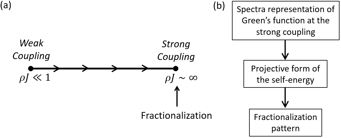
Figure 6: (a) The renormalization group flow for the single-channel Kondo problem. Fractionalization is a property of the strong coupling fixed point. (b) The logic followed in this section. We first use the Lehman representation to find the Green’s function at strong coupling. Then use the latter to extract the self-energy which has a projective form. And finally, having obtained the self-energy we can read off the fractionalization pattern from the strong coupling Hamiltonian.

We begin with the one channel model, demonstrating that self-energy has a sharp pole $\Sigma(z)=V^{2}/z$, that the composite operator $(\vec{\sigma}\cdot\vec{S})_{\alpha\beta}\psi_{\beta}\equiv Vf_{\alpha}$. Next, we consider the an extension of the single-channel Kondo model known as the compactified two-channel Kondo model Coleman et al. (1995), in which the conduction sea has an SO(4)$\sim$SU(2)$\times$SU(2) symmetry. By breaking this symmetry down to an SO(3) subgroup, we are able to demonstrate the fractionalization of the spin into Majorana fermions, giving rise to an odd-frequency triplet state.

.4.1 Fractionalization in the strong coupling limit of single-channel Kondo model

The strong coupling Kondo lattice is literally just the interaction term in the Kondo model

$$H=J(\psi^{\dagger}\vec{\sigma}\psi)\cdot\vec{S}$$ (37)

where we use the notation $\psi^{\dagger}\equiv(\psi^{\dagger}_{\uparrow},\psi^{\dagger}_{\downarrow})$. This is a trivial problem, but we can gain some interesting insight into the nature of composite fermions. We can write this Hamiltonian as $H/J=\left(\vec{S}_{\psi}+\vec{S}\right)^{2}-(\vec{S}_{\psi})^{2}-\frac{3}{4}$, with eigenvalues $E=-3J/2$, $E=J/2$ for the singlet and triplet respectively, and $E=0$ for the empty and doubly occupied conduction electron states. The Hilbert space of energy eigenstates $\{|\lambda\rangle\}$ contains the ground-state

$$|\phi\rangle=\frac{1}{\sqrt{2}}\left(\psi^{\dagger}_{\downarrow}|\Uparrow\rangle-\psi^{\dagger}_{\uparrow}|\Downarrow\rangle\right),\qquad E_{\phi}=-\frac{3}{2}J$$ (38)

the empty and doublet occupied states,

$$\left.\begin{array}[]{rcl}|\sigma\rangle&=&\{|\Uparrow\rangle,|\Downarrow\rangle\},\cr|2,\sigma\rangle&=&\{|2,\Uparrow\rangle,|2,\Downarrow\rangle\}=\{\psi^{\dagger}_{\uparrow}\psi^{\dagger}_{\downarrow}|\Uparrow\rangle,\psi^{\dagger}_{\uparrow}\psi^{\dagger}_{\downarrow}|\Downarrow\rangle\},\end{array}\right\}\qquad E_{\sigma}=0$$ (39)

and the triplet states

$$\left.\begin{array}[]{rcl}|t,m_{J}=+1\rangle&=&\psi^{\dagger}_{\uparrow}|\Uparrow\rangle\cr|t,m_{J}=0\rangle&=&\frac{1}{\sqrt{2}}\left(\psi^{\dagger}_{\uparrow}|\Downarrow\rangle+\psi^{\dagger}_{\downarrow}|\Uparrow\rangle\right)\cr|t,m_{J}=-1\rangle&=&\psi^{\dagger}_{\downarrow}|\Downarrow\rangle\end{array}\right\},\qquad E_{t}=\frac{J}{2}$$ (40)

We can use the Lehmann representation to compute the electron Green’s function, writing

$$G_{c}(z) = \sum_{\lambda}\left[\frac{|\langle\lambda|\psi^{\dagger}_{\sigma}|\phi\rangle|^{2}}{z-(E_{\lambda}-E_{\phi})}+\frac{|\langle\lambda|\psi_{\bar{\sigma}}|\phi\rangle|^{2}}{z-(E_{\phi})-E_{\lambda}}\right]$$ (41)

$$= \left[\frac{|\langle 2,\sigma|\psi^{\dagger}_{\sigma}|\phi\rangle|^{2}}{z-(E_{\lambda}-E_{\phi})}+\frac{|\langle\sigma|\psi_{\bar{\sigma}}|\phi\rangle|^{2}}{z-(E_{\phi})-E_{\lambda}}\right].$$ (42)

where the simplification occurs because the creation and annihilation operators only link the ground-state with the doubly occupied and empty states, respectively. We can use the matrix elements

$$\langle 2,\sigma|\psi^{\dagger}_{\sigma^{\prime}}|\phi\rangle = \frac{1}{\sqrt{2}}\delta_{\sigma\sigma^{\prime}},$$ (43)

$$\langle\sigma|\psi_{\bar{\sigma}^{\prime}}|\phi\rangle = -\frac{1}{\sqrt{2}}\delta_{\sigma\sigma^{\prime}}.$$ (44)

to obtain

$$G_{c}(z)=\frac{1}{2}\left[\frac{1}{z-\frac{3J}{2}}+\frac{1}{z+\frac{3J}{2}}\right]=\frac{z}{z^{2}-(3J/2)^{2}}=\frac{1}{z-\Sigma(z)}$$ (45)

where

$$\Sigma(z)=\frac{(3J/2)^{2}}{z}\equiv\frac{V^{2}}{z}.$$ (46)

thus demonstrating the presence of a sharp pole in the electron self energy with “hybridization” $V=3J/2$. The form of this self-energy is consistent with the identification

$$J(\vec{\sigma}_{\alpha\beta}\cdot\contraction{}{\vec{S}}{)}{c}\vec{S})\psi_{\beta}=V\hat{f}_{\alpha}.$$ (47)

where $V=3J/2$. This strong coupling analysis can be extended in two ways which we leave for a separate publication and just mention the result: a) by aplying a magnetic field to the spin, it can be shown that the action of the spin operator $\vec{S}$ on the ground-state is described by $\vec{S}\equiv f^{\dagger}\frac{\vec{\sigma}}{2}f$. b) by perturbatively including the effect of the kinetic Hamiltinian of the conduction band, it can be shown that the $c$ and the emergent $f$-electrons have a simple two-band effective Hamiltonian at low-energies.

.4.2 Majorana Fractionalization

Next, we look at the strong coupling regime of the so-called compactified two-channel Kondo problem Coleman et al. (1995).

$$H_{int}=J\tilde{\psi}^{\dagger}[\vec{\sigma}+(1-\epsilon)\vec{\tau}]\tilde{\psi}\cdot\vec{S},\qquad\qquad\tilde{\psi}^{\dagger}\equiv\left(\begin{array}[]{cccc}\psi^{\dagger}_{\uparrow}&\psi^{\dagger}_{\downarrow}&\psi^{\vphantom{\dagger}}_{\downarrow}&-\psi^{\vphantom{\dagger}}_{\uparrow}\end{array}\right)$$ (48)

Here, $\tilde{\psi}^{\dagger}\vec{\sigma}\tilde{\psi}$ and $\tilde{\psi}^{\dagger}\vec{\tau}\tilde{\psi}$ are the spin and isospin densities of the conduction electrons and

$$\frac{1}{2}\tilde{\psi}^{\dagger}\vec{\tau}\tilde{\psi}\cdot S=(\psi^{\dagger}_{\uparrow}\psi^{\vphantom{\dagger}}_{\uparrow}+\psi^{\dagger}_{\downarrow}\psi^{\vphantom{\dagger}}_{\downarrow})S^{z}+(\psi^{\dagger}_{\uparrow}\psi^{\dagger}_{\downarrow}S^{-}+h.c.)$$ (49)

For $\epsilon\to 1$ this is just a perturbation of the single-channel Kondo impurity: Near the strong coupling fixed point, the second term is irrelevant because the site near the spin impurity cannot contain both spin and isospin. However, there is a quantum critical point Bulla and Hewson (1997) at $\epsilon=0$ analogous to the two-channel Kondo problem, which happens at strong coupling $J\to\infty$.

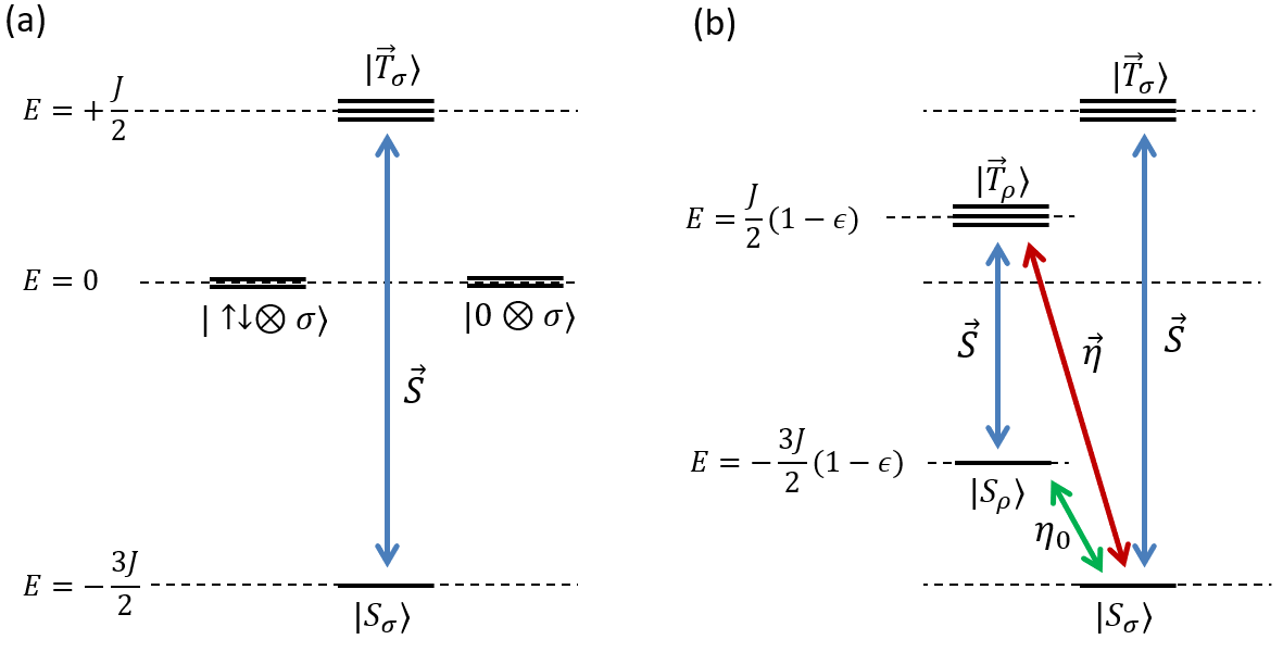
Figure 7: The energy diagram for a single-site problems. (a) Single-channel Kondo problem (b) The compactified two-channel Kondo problem. The arrows show the effect of acting with various operators on the ground state.

The local Hilbert space of the single-channel Kondo problem is composed of the 8 states. In the usual Kondo problem, the Kondo interaction mixes spin states into spin-singlet $\left|S_{\sigma}\right\rangle$ and spin-triplets $\left|\vec{T}_{\sigma}\right\rangle$ separated by an energy gap of $2J$, while the doubly occupied and empty states remain at zero energy [Fig. 7(a)]. In the comapctifie 2CK model, the empty and doubly occipied states are also mixed to create the charge-singlet and charge-triplets states:

$$\left|S_{\rho}\right\rangle=\frac{\left|\Uparrow 0\right\rangle-\left|\Downarrow\uparrow\downarrow\right\rangle}{\sqrt{2}},\qquad\left|T^{0}_{\rho}\right\rangle=\frac{\left|\Uparrow 0\right\rangle+\left|\Downarrow\uparrow\downarrow\right\rangle}{\sqrt{2}},\qquad\left|T^{+}_{\rho}\right\rangle=\left|\Uparrow\uparrow\downarrow\right\rangle,\qquad\left|T^{-}_{\rho}\right\rangle=\left|\Downarrow 0\right\rangle$$

as shown in Fig. 7(b). This problem is best treated in the Majorana representation. We can introduce four Majorana fermions $\gamma_{0}$ and $\vec{\gamma}$ via

$$\left(\begin{array}[]{cc}\psi_{\uparrow}\\ \psi_{\downarrow}\end{array}\right)=\frac{1}{\sqrt{2}}[\gamma_{0}-i\vec{\sigma}\cdot\vec{\gamma}]\left(\begin{array}[]{cc}0\\ i\end{array}\right)=\frac{1}{\sqrt{2}}\left(\begin{array}[]{cc}\gamma^{x}-i\gamma^{y}\\ -\gamma^{z}+i\gamma^{0}\end{array}\right)$$ (50)

$\gamma_{0}$ and $\vec{\gamma}$ are conduction band Majorana fermions that transform as a scalar and vector under SU(2) transformation. There is a freedom on assigning Majorana-s to the Dirac (i.e. complex) fermions, which is reflected by the choice of the spinor on the right. For this choice, we have

$$\tilde{\psi}^{\dagger}\vec{\sigma}\tilde{\psi}=i(-\gamma_{0}\vec{\gamma}-\frac{1}{2}\vec{\gamma}\times\vec{\gamma}),\qquad\tilde{\psi}^{\dagger}\vec{\tau}\tilde{\psi}=i(\gamma_{0}\vec{\gamma}-\frac{1}{2}\vec{\gamma}\times\vec{\gamma})$$ (51)

which leads to

$$H_{int}=-iJ[\epsilon\gamma_{0}\vec{\gamma}+\frac{1}{2}(2-\epsilon)\vec{\gamma}\times\vec{\gamma}]\cdot\vec{S}$$ (52)

Using the zero-temperature spectral representation for the Green’s function

$$G_{\alpha\beta}(z)=\sum_{\lambda}\Big{[}\frac{\left\langle g|\gamma_{\alpha}|\lambda\right\rangle\left\langle\lambda|\gamma_{\beta}|g\right\rangle}{z-(E_{\lambda}-E_{g})}+\frac{\left\langle\lambda|\gamma_{\alpha}|g\right\rangle\left\langle g|\gamma_{\beta}|\lambda\right\rangle}{z+(E_{\lambda}-E_{g})}\Big{]}$$ (53)

and the matrix elements indicated in Fig. 7(b) find

$$G_{\alpha\beta}(z)=\frac{P^{S}_{\alpha\beta}}{z-\Delta E_{S}/z}+\frac{P^{T}_{\alpha\beta}}{z-\Delta E_{T}/z}$$ (54)

where in this Majorana basis we have $P^{S}_{\alpha\beta}=\delta_{\alpha\beta}\delta_{\alpha,0}$ and $P^{T}_{\alpha\beta}=\delta_{\alpha\beta}-P^{S}_{\alpha\beta}$, and

$$\Delta E_{S}=\frac{3J}{2}\epsilon,\qquad\Delta E_{T}=\frac{J}{2}(4-\epsilon).$$ (55)

This means we can write the self-energy as

$$\Sigma_{\alpha\beta}(z)=P_{\alpha\beta}^{S}\frac{\Delta E_{S}}{z}+P_{\alpha\beta}^{T}\frac{\Delta E_{T}}{z}$$ (56)

Note that in the limit of $\epsilon\to 1$ this expression reduces to the original single-channel self-energy. On the other-hand in the limit of $\epsilon\to 0$ the singlet contribution drops out.

Having the structure of the self-energy, we can work out the fractionalization pattern by which the conduction electron Majoranas combine with the spin. The contractions allowed by the symmetry are

$$\contraction[1ex]{}{\gamma_{0}}{}{S^{a}}\gamma_{0}S^{a}\to A\eta^{a},\qquad\contraction[1ex]{}{\gamma^{a}}{}{S^{b}}\gamma^{a}S^{b}\to\delta^{ab}B\eta_{0}+\epsilon^{abc}C\eta^{c}.$$ (57)

in terms of emergent localized Majorana fermions $\eta_{0}$ and $\vec{\eta}$. Using these in Eq. (52) we find

$$H_{int}\to-iJ\Big{\{}\Big{[}2C(2-\epsilon)-A\epsilon\Big{]}\vec{\gamma}\cdot\vec{\eta}+3B\epsilon\gamma_{0}\eta_{0}\Big{\}}$$ (58)

and comparing it to the projective self-energy, the coefficients can be read off as

$$B=\frac{1}{2},\qquad A=-\frac{1}{2},\qquad C=\frac{1}{2}.$$ (59)

Especially, at the $\epsilon\to 0$ we recover the fractionalization pattern reported in the entry a’ of the table in the main section.

.5 Analysis of SO(5) symmetry breaking in the two-channel Kondo model

Finally, we turn to the usual two channel Kondo model (Fig. 8) which has a continuous channel-charge SP (4) and spin SU(2) symmetry, SP(4)$\times$ SU(2).

In the paper we used NRG to induce order fractionalization in an impurity with channel asymmetry

$$H=\sum_{\alpha}\psi^{\dagger}_{\alpha}(\vec{\sigma}\cdot\vec{S})[J+\delta J\alpha^{z}]\psi_{\alpha}.$$ (60)

At the strong coupling, the self-energy is only induced in the stronger channel. This is consistent with the the RG flow (Fig. 8a) which imply that $J,\delta J\to\infty$ and $\delta J/J\to 1$ so that the Hamiltonian takes the same projective form as the self-energy.

We also argued that since the channel symmetry is a continuous group, we may induce order fractionalization using the relevant perturbation

$$H=\sum_{\alpha}\psi^{\dagger}_{\alpha}(\vec{\sigma}\cdot\vec{S})[J+\delta J\vec{n}\cdot\vec{\alpha}]\psi_{\alpha}.$$ (61)

At the strong coupling fixed point the self-energy is only induced in the stronger channel, leading to a projective form for the self-energy

$$\Sigma_{\lambda\lambda^{\prime}}(z)=V^{2}\frac{P_{\lambda\lambda}}{z},\qquad P=\frac{1}{2}(1+\vec{n}\cdot\vec{\alpha})$$ (62)

and the fractionalization pattern

$$J(\vec{\sigma}\cdot\vec{S})\psi_{\alpha}=V_{\lambda}f,$$ (63)

where $\psi_{\alpha}$ with $\alpha=1,2$ and $f$ are regarded as spinors in spin-space and $(\vec{n}\cdot\alpha)V_{\lambda}=+V_{\lambda}$.

In this section, we first review the symmetry properties of the two-channel Kondo model, showing that the channel symmetry is part of a larger channel-charge SP(4) symmetry. The fully symmetry of the two-channel Kondo problem is SO(3)$\times$ SO(5) or SU(2)$\times$SP(4) Affleck et al. (1992). It turns out that there is a full family of projection operators, which enables us to describe a family of different fractionalization patterns (Fig. 8b).

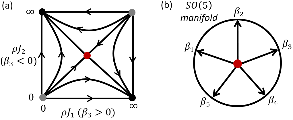
Figure 8: (a) The renormalization group flow for the two-channel Kondo problem in the space of Kondo couplings of the two channel. The critical fixed point (red) is sensitive to the channel asymmetry and flows to stable fixed points (black). (b) More general representation of the symmetry breaking; the critical finite-coupling fixed point of the two-channel Kondo lattice can be (explicitly or spontaneously) broken into any point on the SO(5) manifold.

.5.1 SP(4) symmetry of the two-channel Kondo problem

In order to see this, note that the Kondo interaction can be written as Affleck et al. (1988)

$$H_{int}=\frac{J}{4}{\rm Tr}\Big{[}\Psi^{\dagger}\Psi\vec{\sigma}^{T}\cdot\vec{S}\Big{]}$$ (64)

where we have arranged the elements of $\tilde{\psi}$ in a 4$\times$2 matrix

$$\Psi_{\lambda,\sigma}=\left(\begin{array}[]{c|c}\psi_{1\uparrow}&\psi_{1\downarrow}\\ \psi_{2\uparrow}&\psi_{2\downarrow}\\ \hline\cr-\psi^{\dagger}_{2\downarrow}&\psi^{\dagger}_{2\uparrow}\\ \psi^{\dagger}_{1\downarrow}&-\psi^{\dagger}_{1\uparrow}\end{array}\right)$$ (65)

Despite its formidable form, different symmetries of the problem are manifest in this representation. The quantum number $\sigma=\uparrow,\downarrow$ is connected to the column, whereas the quantum number $\lambda=[\alpha,\tau]$ connected to the rows is a super-index characterizing channel $\alpha=1,2$ and the isospin $\tau=e,h$ degrees of freedom. The isospin tags the large blocks whereas channel tags internal structure of the blocks. Associated with each of these quantum numbers, there exist Pauli matrices $\vec{\sigma}$ acting from the right side and Pauli matrices $\vec{\alpha}$ and $\vec{\tau}$ acting from the left side. The Kondo interaction, as well as the commutation relations and the kinetic energy are invariant under separate left and right transformations of $\psi$:

$$\Psi\to g\Psi,\qquad\Psi\to\Psi h$$ (66)

where $h=e^{i\vec{\phi}\cdot\vec{\sigma}}$ is a usual SU(2) transformation, but $g$ is an element of SP(4) parametrized by

$${\rm SP(4)}:\qquad g=e^{i\sum_{m=1}^{10}\theta_{j}\Lambda_{j}},\qquad\Lambda_{j}\in\{\vec{\alpha},\vec{\alpha}\tau_{1},\vec{\alpha}\tau_{2},\tau_{3}\}.$$ (67)

Proof: Naively, for any SU(4) and SU(2) transformation can be used in Eq. (66). However, our description Eq. (68) has a redundancy, that implies invariance under the discrete transformation

$$\tilde{\psi}\to\theta_{L}\tilde{\psi}^{*}\theta_{R},\qquad\theta_{L}=i\alpha_{2}\tau_{1},\qquad\theta_{R}=i\sigma_{2}$$ (68)

that needs to remain consistent under unitary transformations. For the left transformation, this means

$$g\theta_{L}\tilde{\psi}^{*}\theta_{R}=\theta_{L}(g\tilde{\psi})^{*}\theta_{R},\qquad\rightarrow\qquad g\theta_{L}=\theta_{L}g^{*}$$ (69)

The SU(4) transformation can be generated by the generators $\Lambda_{jk}=\alpha_{j}\tau_{k}$. Considering a group element $g$ to $g=e^{i\Lambda}$ in terms of generators $\Lambda=\sum_{jk}d_{jk}\Lambda_{jk}$, with infinitesimal arbitrary $d_{jk}$, we conclude

$$\Lambda=\theta_{L}\Lambda^{T}\theta_{L}$$ (70)

which is the defining equation for symplectic representation SP(4). The subset of generators that satisfy this condition are the 10 generators given in Eq. (67). This is the same number of generators as SO(5) and indeed it can be shown that SP(4) id a double cover of SO(5). The discrete symmetry (68) is not restrictive for the right-transformation, because it requires

$$\theta_{R}h=h^{*}\theta_{R}$$ (71)

which in terms of infinitesimal group element $g=e^{i\Gamma}$ with $\Gamma=\sum_{j}d_{j}\sigma_{j}$ leads to

$$\Gamma^{T}\theta_{R}+\Gamma\theta_{R}=0$$ (72)

All Pauli matrices satisfy this condition and so the $h$-transformations remain SU(2).

.5.2 The projective form of the self-energy

The 10 generators $\Lambda_{j}\in$ SP(4) are a subset of the 15 generators of SU(4). Out of the remaining 5 generators that are not part of $g\in SP(4)$ we can build a family of projectors

$${\cal P}=\frac{1}{2}\Big{(}1+\vec{m}\cdot\vec{\beta}\Big{)},\qquad\vec{\beta}=\{\alpha_{1}\tau_{3},\alpha_{2}\tau_{3},\alpha_{3}\tau_{3},\tau_{1},\tau_{2}\},$$ (73)

parametrized by the 5 component vector $\vec{m}$. The important point is that these projectors rotate among themselves by the elements of $g\in$SP(4) group:

$$g^{\dagger}(\vec{m}\cdot\vec{\beta})g=\vec{m}^{\prime}\cdot\vec{\beta}.$$ (74)

The channel symmetry breaking perturbations discussed in Eqs. 60 and 61 correspond to $\alpha_{3}\tau_{3}$ and $\vec{\alpha}\tau_{3}$, respectively. Since, different projectors can be rotated into each other, for the most general case of Eq. 73 the self-energy has the projective form

$$\Sigma(z)=\frac{V^{2}}{z}{\cal P}.$$ (75)

in the $\Psi$ representation. To extract the patterns of fractionalization, we first find eigenvectors of $\cal P$, i.e. look for unit vectors $z$ that satisfy

$$(\vec{m}\cdot\vec{\beta}){\rm z}={\rm z}$$ (76)

with $z^{\dagger}z=1$. Such an eigenvector enables a CP³ representation of the five-component $\vec{m}$ vector through $\vec{m}={\rm z}^{\dagger}\vec{\beta}{\rm z}$. These eigenvectors have the general form

$${\rm z}=\left(\begin{array}[]{cc}u_{1}\\ u_{2}\\ -\bar{v}_{2}\\ v_{2}\end{array}\right).$$ (77)

It turns out that ${\cal P}$ has a symmetry

$$\epsilon_{4}^{T}(\vec{m}\cdot\vec{\beta})\epsilon_{4}=\vec{m}\cdot\vec{\beta}$$ (78)

where $\epsilon_{4}=i\alpha_{2}\tau_{1}$ is the fully antisymmetric matrix. It follows that both ${\rm z}$ and $\epsilon_{4}{\rm z}^{*}$ are degenerate eigenvectors of ${\cal P}$ with eigenvalue +1:

$$(\vec{m}\cdot\vec{\beta})(\epsilon_{4}{\rm z}^{*})=(\epsilon_{4}{\rm z}^{*}).$$ (79)

These two can be combined into a single matrix

$${\cal Z}_{\lambda\tau}=\left(\begin{array}[]{cc}{\rm z}&\epsilon_{4}{\rm z}^{*}\end{array}\right)=\left(\begin{array}[]{c|c}u_{1}&v_{1}\\ u_{2}&v_{2}\\ \hline\cr-\bar{v}_{2}&\bar{u}_{2}\\ \bar{v}_{1}&-\bar{u}_{1}\end{array}\right)=g\left(\begin{array}[]{c|c}1&0\\ 0&0\\ \hline\cr 0&0\\ 0&1\end{array}\right)$$ (80)

Here, $\lambda$ index corresponds to the rows and the eigenvectors are enumerated by the coulomn $\tau$ index. The second equation highlights that the general ${\cal Z}$ eigen-matrix can be obtained form a SP(4) rotation of a reference ${\cal Z}$ eigen-matrix, corresponding to the projector $\beta=\alpha_{3}\tau_{3}$ used in the NRG.

Writing ${\rm z}=\left\langle\lambda|\tau=1\right\rangle$ and $\epsilon_{4}{\rm z}^{*}=\left\langle\lambda|\tau=2\right\rangle$ the projector has the form ${\cal P}=\sum_{\tau=1,2}\left|\tau\right\rangle\left\langle\tau\right|$ or in components:

$${\cal P}_{\lambda\lambda^{\prime}}=\sum_{\tau=1,2}\left\langle\lambda|\tau\right\rangle\left\langle\tau|\lambda^{\prime}\right\rangle={\cal Z}^{\vphantom{\dagger}}_{\lambda\tau}{\cal Z}^{*}_{\lambda^{\prime}\tau}.$$ (81)

and the self-energy will take the form

$$\Sigma_{\lambda\lambda^{\prime}}(z)=\frac{V^{2}}{z}({\cal Z}{\cal Z}^{\dagger})_{\lambda\lambda^{\prime}}$$ (82)

and has an internal SU(2) gauge invariance under ${\cal Z}\to{\cal Z}h$ where $h\in SU(2)$.

.5.3 Fractionalization pattern and composite ordering

In terms of $\Psi$ matrix the Hamiltonian is

$$H=\frac{J}{4}{\rm Tr}\Big{[}\Psi^{\dagger}{\cal P}\Psi(\vec{\sigma}^{T}\cdot S)\Big{]}.$$ (83)

and Eq. (63) can be written as

$$J\Psi(\vec{\sigma}^{T}\cdot\vec{S})={\cal V}{\cal F},\qquad\qquad\qquad\tilde{\cal F}=\left(\begin{array}[]{cc}f_{\uparrow}&f_{\downarrow}\\ f^{\dagger}_{\downarrow}&-f^{\dagger}_{\uparrow}\end{array}\right),$$ (84)

where ${\cal V}=V{\cal Z}$. Using the notation $Vu_{\lambda}\to V_{\lambda}$ and $Vv_{\lambda}\to\Delta_{\lambda}$ in the general expression for $\cal Z$ in Eq. (80) and translating the above equation back to the $\psi$ spinors, the contraction reads

$$J(\vec{\sigma}\cdot\vec{S})_{\alpha\beta}\psi_{\lambda\sigma}=V_{\lambda}f_{\alpha}+\Delta_{\lambda}f^{\dagger}_{-\alpha}{\rm sign}{(}\alpha)$$ (85)

which is nothing but the composite pairing Hoshino and Kuramoto (2015). In particular the conduction electron self-energy contains Andreev reflections. This is not surprising given that here, we have induced the symmetry breaking in the pairing channel. As explained in the manuscript, we conjecture that this symmetry breaking and the associated fractionalizations can happen spontaneously in a lattice.

References

- Zaanen et al. (2006) J. Zaanen, S. Chakravarty, T Senthil, P. W. Anderson, P. A. Lee, J. Schmalian, M. Imada, D. Pines, M. Randeria, C. M. Varma, M. Vojta, and T. M. Rice, “Towards a complete theory of high Tc,” Nature Physics 2, 138–143 (2006).
- Lee et al. (2006) Patrick A. Lee, Naoto Nagaosa, and Xiao-Gang Wen, “Doping a Mott insulator: Physics of high-temperature superconductivity,” Rev. Mod. Phys. 78, 17–85 (2006).
- Si et al. (2016) Qimiao Si, Rong Yu, and Elihu Abrahams, “High-temperature Superconductivity in Iron Pnictides and Chalcogenides,” Nature Reviews Materials 1, 16017 (2016).
- Moore (2010) Joel E Moore, “The birth of Topological Insulators,” Nature 464, 194–198 (2010).
- Qi and Zhang (2011) Xiao-Liang Qi and Shou-Cheng Zhang, “Topological Insulators and Superconductors,” Rev. Mod. Phys. 83, 1057–1110 (2011).
- Hasan and Kane (2010) M. Z. Hasan and C. L. Kane, “Colloquium: Topological insulators,” Rev. Mod. Phys. 82, 3045–3067 (2010).
- Savary and Balents (2017) Lucile Savary and Leon Balents, “Quantum Spin Liquids: a review,” Reports on Progress in Physics 80, 016502 (2017).
- Zhou et al. (2017) Yi Zhou, Kazushi Kanoda, and Tai-Kai Ng, “Quantum Spin Liquid States,” Rev. Mod. Phys. 89, 025003 (2017).
- Landau (1937) L. D. Landau, “ Theory of Phase Transformations,” Phys. Z. SowjUn 11, 545 (1937).
- Yang (1962) C. N. Yang, “ Concept of Off-Diagonal Long-Range Order and the Quantum Phases of Liquid He and of Superconductors,” Rev. Mod. Phys. 34, 694–704 (1962).
- Pauli (1940) W. Pauli, “The connection between spin and statistics,” Phys. Rev. 58, 716–722 (1940).
- Duck and Sudarshan (1998) Ian Duck and E C G Sudarshan, “Toward an understanding of the spin-statistics theorem,” American Journal of Physics 66, 284–303 (1998).