Bayesian graph convolutional neural networks for semi-supervised classification

Abstract

Recently, techniques for applying convolutional neural networks to graph-structured data have emerged. Graph convolutional neural networks (GCNNs) have been used to address node and graph classification and matrix completion. Although the performance has been impressive, the current implementations have limited capability to incorporate uncertainty in the graph structure. Almost all GCNNs process a graph as though it is a ground-truth depiction of the relationship between nodes, but often the graphs employed in applications are themselves derived from noisy data or modelling assumptions. Spurious edges may be included; other edges may be missing between nodes that have very strong relationships. In this paper we adopt a Bayesian approach, viewing the observed graph as a realization from a parametric family of random graphs. We then target inference of the joint posterior of the random graph parameters and the node (or graph) labels. We present the Bayesian GCNN framework and develop an iterative learning procedure for the case of assortative mixed-membership stochastic block models. We present the results of experiments that demonstrate that the Bayesian formulation can provide better performance when there are very few labels available during the training process.

1 Introduction

Novel approaches for applying convolutional neural networks to graph-structured data have emerged in recent years. Commencing with the work in (?; ?), there have been numerous developments and improvements. Although these graph convolutional neural networks (GCNNs) are promising, the current implementations have limited capability to handle uncertainty in the graph structure, and treat the graph topology as ground-truth information. This in turn leads to an inability to adequately characterize the uncertainty in the predictions made by the neural network.

In contrast to this past work, we employ a Bayesian framework and view the observed graph as a realization from a parametric random graph family. The observed adjacency matrix is then used in conjunction with features and labels to perform joint inference. The results reported in this paper suggest that this formulation, although computationally more demanding, can lead to an ability to learn more from less data, a better capacity to represent uncertainty, and better robustness and resilience to noise or adversarial attacks.

In this paper, we present the novel Bayesian GCNN framework and discuss how inference can be performed. To provide a concrete example of the approach, we focus on a specific random graph model, the assortative mixed membership block model. We address the task of semi-supervised classification of nodes and examine the resilience of the derived architecture to random perturbations of the graph topology.

2 Related work

A significant body of research focuses on using neural networks to analyze structured data when there is an underlying graph describing the relationship between data items. Early work led to the development of the graph neural network (GNN) (?; ?; ?). The GNN approaches rely on recursive processing and propagation of information across the graph. Training can often take a long time to converge and the required time scales undesirably with respect to the number of nodes in the graph, although recently an approach to mitigate this has been proposed by (?).

Graph convolutional neural networks (GCNNs) have emerged more recently, with the first proposals in (?; ?; ?). A spectral filtering approach was introduced in (?) and this method was simplified or improved in (?; ?; ?). Spatial filtering or aggregation strategies were adopted in (?; ?). A general framework for training neural networks on graphs and manifolds was presented by (?) and the authors explain how several of the other methods can be interpreted as special cases.

The performance of the GCNNs can be improved by incorporating attention nodes (?), leading to the graph attention network (GAT). Experiments have also demonstrated that gates, edge conditioning, and skip connections can prove beneficial (?; ?; ?). In some problem settings it is also beneficial to consider an ensemble of graphs (?), multiple adjacency matrices (?) or the dual graph (?). Compared to this past work, the primary methodological novelty in our proposed approach involves the adoption of a Bayesian framework and the treatment of the observed graph as additional data to be used during inference.

There is a rich literature on Bayesian neural networks, commencing with pioneering work (?; ?; ?; ?) and extending to more recent contributions (?; ?; ?; ?). To the best of our knowledge, Bayesian neural networks have not yet been developed for the analysis of data on graphs.

3 Background

Graph convolutional neural networks (GCNNs)

Although graph convolutional neural networks can be applied to a variety of inference tasks, in order to make the description more concrete we consider the task of identifying the labels of nodes in a graph. Suppose that we observe a graph $\mathcal{G}_{obs}=(\mathcal{V},\mathcal{E})$, comprised of a set of $N$ nodes $\mathcal{V}$ and a set of edges $\mathcal{E}$. For each node we measure data (or derive features), denoted $\bm{x}_{i}$ for node $i$. For some subset of the nodes $\mathcal{L}\subset\mathcal{V}$, we can also measure labels $\mathbf{Y_{\mathcal{L}}}=\{\bm{y}_{i}:i\in\mathcal{L}\}$. In a classification context, the label $\bm{y}_{i}$ identifies a category; in a regression context $\bm{y}_{i}$ can be real-valued. Our task is to use the features $\bm{x}$ and the observed graph structure $\mathcal{G}_{obs}$ to estimate the labels of the unlabelled nodes.

A GCNN performs this task by performing graph convolution operations within a neural network architecture. Collecting the feature vectors as the rows of a matrix $\bm{X}$, the layers of a GCNN (?; ?) are of the form:

$$\mathbf{H}^{(1)} =\sigma(\mathbf{A}_{\mathcal{G}}\mathbf{X}\mathbf{W}^{(0)})$$ (1)

$$\mathbf{H}^{(l+1)} =\sigma(\mathbf{A}_{\mathcal{G}}\mathbf{H}^{(l)}\mathbf{W}^{(l)})$$ (2)

Here $\mathbf{W}^{(l)}$ are the weights of the neural network at layer $l$, $\mathbf{H}^{(l)}$ are the output features from layer $l-1$, and $\sigma$ is a non-linear activation function. The matrix $\mathbf{A}_{\mathcal{G}}$ is derived from the observed graph and determines how the output features are mixed across the graph at each layer. The final output for an $L$-layer network is $\mathbf{Z}=\mathbf{H}^{(L)}$. Training of the weights of the neural network is performed by backpropagation with the goal of minimizing an error metric between the observed labels $\mathbf{Y}$ and the network predictions $\mathbf{Z}$. Performance improvements can be achieved by enhancing the architecture with components that have proved useful for standard CNNs, including attention nodes (?), and skip connections and gates (?; ?).

Although there are many different flavours of GCNNs, all current versions process the graph as though it is a ground-truth depiction of the relationship between nodes. This is despite the fact that in many cases the graphs employed in applications are themselves derived from noisy data or modelling assumptions. Spurious edges may be included; other edges may be missing between nodes that have very strong relationships. Incorporating attention mechanisms as in (?) addresses this to some extent; attention nodes can learn that some edges are not representative of a meaningful relationship and reduce the impact that the nodes have on one another. But the attention mechanisms, for computational expediency, are limited to processing existing edges — they cannot create an edge where one should probably exist. This is also a limitation of the ensemble approach of (?), where learning is performed on multiple graphs derived by erasing some edges in the graph.

Bayesian neural networks

We consider the case where we have training inputs $\mathbf{X}=\{x_{1},...,x_{n}\}$ and corresponding outputs $\mathbf{Y}=\{y_{1},...,y_{n}\}$. Our goal is to learn a function $y=f(x)$ via a neural network with fixed configuration (number of layers, activation function, etc., so that the weights are sufficient statistics for $f$) that provides a likely explanation for the relationship between $x$ and $y$. The weights $W$ are modelled as random variables in a Bayesian approach and we introduce a prior distribution over them. Since $W$ is not deterministic, the output of the neural network is also a random variable. Prediction for a new input $x$ can be formed by integrating with respect to the posterior distribution of $W$ as follows:

$$p(y|x,\mathbf{X},\mathbf{Y})=\int p(y|x,W)p(W|\mathbf{X},\mathbf{Y})\,dW\,.$$ (3)

The term $p(y|x,W)$ can be viewed as a likelihood; in a classification task it is modelled using a categorical distribution by applying a softmax function to the output of the neural network; in a regression task a Gaussian likelihood is often an appropriate choice. The integral in eq. (3) is in general intractable. Various techniques for inference of $p(W|\mathbf{X},\mathbf{Y})$ have been proposed in the literature, including expectation propagation (?), variational inference (?; ?; ?), and Markov Chain Monte Carlo methods (?; ?; ?). In particular, in (?), it was shown that with suitable variational approximation for the posterior of $W$, Monte Carlo dropout is equivalent to drawing samples of $W$ from the approximate posterior and eq. (3) can be approximated by a Monte Carlo integral as follows:

$$p(y|x,\mathbf{X},\mathbf{Y})\approx\dfrac{1}{T}\displaystyle\sum_{i=1}^{S}p(y|x,W_{i})\,,$$ (4)

where $S$ weights $W_{i}$ are obtained via dropout.

4 Methodology

We consider a Bayesian approach, viewing the observed graph as a realization from a parametric family of random graphs. We then target inference of the joint posterior of the random graph parameters, weights in the GCNN and the node (or graph) labels. Since we are usually not directly interested in inferring the graph parameters, posterior estimates of the labels are obtained by marginalization. The goal is to compute the posterior probability of labels, which can be written as:

$$p(\mathbf{Z}|\mathbf{Y_{\mathcal{L}}},\mathbf{X},\mathcal{G}_{obs}) =\int p(\mathbf{Z}|W,\mathcal{G},\mathbf{X})p(W|\mathbf{Y_{\mathcal{L}}},\mathbf{X},\mathcal{G})\,$$

$$\quad\quad p(\mathcal{G}|\lambda)p(\lambda|\mathcal{G}_{obs})\,dW\,d\mathcal{G}\,d\lambda\,.$$ (5)

Here $W$ is a random variable representing the weights of a Bayesian GCNN over graph $\mathcal{G}$, and $\lambda$ denotes the parameters that characterize a family of random graphs. The term $p(\mathbf{Z}|W,\mathcal{G},\mathbf{X})$ can be modelled using a categorical distribution by applying a softmax function to the output of the GCNN, as discussed above.

This integral in eq. (5) is intractable. We can adopt a number of strategies to approximate it, including variational methods and Markov Chain Monte Carlo (MCMC). For example, in order to approximate the posterior of weights $p(W|\mathbf{Y_{\mathcal{L}}},\mathbf{X},\mathcal{G})$, we could use variational inference (?; ?; ?) or MCMC (?; ?; ?). Various parametric random graph generation models can be used to model $p(\lambda|\mathcal{G}_{obs})$, for example a stochastic block model (?), a mixed membership stochastic block model (?), or a degree corrected block model (?). For inference of $p(\lambda|\mathcal{G}_{obs})$, we can use MCMC (?) or variational inference (?).

A Monte Carlo approximation of eq. (5) is:

$$p(\mathbf{Z}|\mathbf{Y_{\mathcal{L}}},\mathbf{X},\mathcal{G}_{obs})\approx$$

$$\quad\quad\quad\dfrac{1}{V}\sum_{v}^{V}\dfrac{1}{N_{G}S}\sum_{i=1}^{N_{G}}\sum_{s=1}^{S}p(\mathbf{Z}|W_{s,i,v},\mathcal{G}_{i,v},\mathbf{X})\,.$$ (6)

In this approximation, $V$ samples $\lambda_{v}$ are drawn from $p(\lambda|\mathcal{G}_{obs})$; the precise method for generating these samples from the posterior varies depending on the nature of the graph model. The $N_{G}$ graphs $\mathcal{G}_{i,v}$ are sampled from $p(\mathcal{G}|\lambda_{v})$ using the adopted random graph model. $S$ weight matrices $W_{s,i,v}$ are sampled from $p(W|\mathbf{Y_{\mathcal{L}}},\mathbf{X},\mathcal{G}_{i,v})$ from the Bayesian GCN corresponding to the graph $\mathcal{G}_{i,v}$.

Example: Assortative mixed membership stochastic block model

For the Bayesian GCNNs derived in this paper, we use an assortative mixed membership stochastic block model (a-MMSBM) for the graph (?; ?) and learn its parameters $\lambda=\{\pi,\beta\}$ using a stochastic optimization approach. The assortative MMSBM, described in the following section, is a good choice to model a graph that has relatively strong community structure (such as the citation networks we study in the experiments section). It generalizes the stochastic block model by allowing nodes to belong to more than one community and to exhibit assortative behaviour, in the sense that a node can be connected to one neighbour because of a relationship through community A and to another neighbour because of a relationship through community B.

Since $\mathcal{G}_{obs}$ is often noisy and may not fit the adopted parametric block model well, sampling $\pi_{v}$ and $\beta_{v}$ from $p(\pi,\beta|\mathcal{G}_{obs})$ can lead to high variance. This can lead to the sampled graphs $\mathcal{G}_{i,v}$ being very different from $\mathcal{G}_{obs}$. Instead, we replace the integration over $\pi$ and $\beta$ with a maximum a posteriori estimate (?). We approximately compute

$$\{\hat{\pi},\hat{\beta}\} =\arg\max_{\beta,\pi}p(\beta,\pi|\mathcal{G}_{obs})$$ (7)

by incorporating suitable priors over $\beta$ and $\pi$ and use the approximation:

$$p(\mathbf{Z}|\mathbf{Y_{\mathcal{L}}},\mathbf{X},\mathcal{G}_{obs})\approx\dfrac{1}{N_{G}S}\sum_{i=1}^{N_{G}}\sum_{s=1}^{S}p(\mathbf{Z}|W_{s,i},\mathcal{G}_{i},\mathbf{X})\,.$$ (8)

In this approximation, $W_{s,i}$ are approximately sampled from $p(W|\mathbf{Y_{\mathcal{L}}},\mathbf{X},\mathcal{G}_{i})$ using Monte Carlo dropout over the Bayesian GCNN corresponding to $\mathcal{G}_{i}$. The $\mathcal{G}_{i}$ are sampled from $p(\mathcal{G}|\hat{\pi},\hat{\beta})$.

Posterior inference for the MMSBM

For the undirected observed graph $\mathcal{G}_{obs}=\{y_{ab}\in\{0,1\}:1\leq a<b\leq N\}$, $y_{ab}=0$ or $1$ indicates absence or presence of a link between node $a$ and node $b$. In MMSBM, each node $a$ has a $K$ dimensional community membership probability distribution $\pi_{a}=[\pi_{a1},...\pi_{aK}]^{T}$, where $K$ is the number of categories/communities of the nodes. For any two nodes $a$ and $b$, if both of them belong to the same community, then the probability of a link between them is significantly higher than the case where the two nodes belong to different communities (?). The generative model is described as:

For any two nodes $a$ and $b$,

• Sample $z_{ab}\sim\pi_{a}$ and $z_{ba}\sim\pi_{b}$.

• If $z_{ab}=z_{ba}=k$, sample a link $y_{ab}\sim\text{Bernoulli}(\beta_{k})$. Otherwise, $y_{ab}\sim\text{Bernoulli}(\delta)$.

Here, $0\leq\beta_{k}\leq 1$ is termed community strength of the $k$-th community and $\delta$ is the cross community link probability, usually set to a small value. The joint posterior of the parameters $\pi$ and $\beta$ is given as:

$$p(\pi,\beta|\mathcal{G}_{obs})\propto p(\beta)p(\pi)p(\mathcal{G}_{obs}|\pi,\beta)\,$$

$$= \prod_{k=1}^{K}p(\beta_{k})\prod_{a=1}^{N}p(\pi_{a})\prod_{1\leq a<b\leq N}\sum_{z_{ab},z_{ba}}p(y_{ab},z_{ab},z_{ba}|\pi_{a},\pi_{b},\beta)\,.$$ (9)

We use a $\text{Beta}(\eta)$ distribution for the prior of $\beta_{k}$ and a Dirichlet distribution, $\text{Dir}(\alpha)$, for the prior of $\pi_{a}$, where $\eta$ and $\alpha$ are hyper-parameters.

Expanded mean parameterisation

Maximizing the posterior of eq. (9) is a constrained optimization problem with $\beta_{k},\pi_{ak}\in(0,1)$ and $\displaystyle\sum_{k=1}^{K}\pi_{ak}=1$. Employing a standard iterative algorithm with a gradient based update rule does not guarantee that the constraints will be satisfied. Hence we consider an expanded mean parameterisation (?) as follows. We introduce the alternative parameters $\theta_{k0},\theta_{k1}\geq 0$ and adopt as the prior for these parameters a product of independent $\text{Gamma}(\eta,\rho)$ distributions. These parameters are related to the original parameter $\beta_{k}$ through the relationship $\beta_{k}=\dfrac{\theta_{k1}}{\theta_{k0}+\theta_{k1}}$. This results in a $\text{Beta}(\eta)$ prior for $\beta_{k}$. Similarly, we introduce a new parameter $\phi_{a}\in\mathbb{R}^{K}_{+}$ and adopt as its prior a product of independent $\text{Gamma}(\alpha,\rho)$ distributions. We define $\pi_{ak}=\dfrac{\phi_{ak}}{\displaystyle\sum_{l=1}^{K}\phi_{al}}$, which results in a Dirichlet prior, $\text{Dir}(\alpha)$, for $\pi_{a}$. The boundary conditions $\theta_{ki},\phi_{ak}\geq 0$ can be handled by simply taking the absolute value of the update.

Stochastic optimization and mini-batch sampling

We use preconditioned gradient ascent to maximize the joint posterior in eq. (9) over $\theta$ and $\phi$. In many graphs that are appropriately modelled by a stochastic block model, most of the nodes belong strongly to only one of the $K$ communities, so the MAP estimate for many $\pi_{a}$ lies near one of the corners of the probability simplex. This suggests that the scaling of different dimensions of $\phi_{a}$ can be very different. Similarly, as $\mathcal{G}_{obs}$ is typically sparse, the community strengths $\beta_{k}$ are very low, indicating that the scales of $\theta_{k0}$ and $\theta_{k1}$ are very different. We use preconditioning matrices $G(\theta)=\mathrm{diag}(\theta)^{-1}$ and $G(\phi)=\mathrm{diag}(\phi)^{-1}$ as in (?), to obtain the following update rules:

$$\theta_{ki}^{(t+1)} =$$

$$\Big{|}\theta_{ki}^{(t)}+\epsilon_{t}\Big{(}\eta-1-\rho\theta_{ki}^{(t)}+\theta_{ki}^{(t)}\sum_{a=1}^{N}\sum_{b=a+1}^{N}g_{ab}(\theta_{ki}^{(t)})\Big{)}\Big{|}\,,$$ (10)

$$\phi_{ak}^{(t+1)} =\Big{|}\phi_{ak}^{(t)}+\epsilon_{t}\Big{(}\alpha-1-\rho\phi_{ak}^{(t)}\sum_{b=1,b\neq a}^{N}g_{ab}(\phi_{ak}^{(t)})\Big{)}\Big{|}\,,$$ (11)

where $\epsilon_{t}=\epsilon_{0}(t+\tau)^{-\kappa}$ is a decreasing step-size, and $g_{ab}(\theta_{ki})$ and $g_{ab}(\phi_{ak})$ are the partial derivatives of $\log p(y_{ab}|\pi_{a},\pi_{b},\beta)$ w.r.t. $\theta_{ki}$ and $\phi_{ak}$, respectively. Detailed expressions for these derivatives are provided in eqs. (9) and (14) of (?).

Implementation of (10) and (11) is $\mathcal{O}(N^{2}K)$ per iteration, where $N$ is the number of nodes in the graph and $K$ the number of communities. This can be prohibitively expensive for large graphs. We instead employ a stochastic gradient based strategy as follows. For update of $\theta_{ki}$’s in eq. (10), we split the $\mathcal{O}(N^{2})$ sum over all edges and non-edges, $\sum_{a=1}^{N}\sum_{b=a+1}^{N}$, into two separate terms. One of these is a sum over all observed edges and the other is a sum over all non-edges. We calculate the term corresponding to observed edges exactly (in the sparse graphs of interest, the number of edges is closer to $\mathcal{O}(N)$ than $\mathcal{O}(N^{2})$). For the other term we consider a mini-batch of 1 percent of randomly sampled non-edges and scale the sum by a factor of 100.

At any single iteration, we update the $\phi_{ak}$ values for only $n$ randomly sampled nodes ($n<N$), keeping the rest of them fixed. For the update of $\phi_{ak}$ values of any of the randomly selected $n$ nodes, we split the sum in eq. (11) into two terms. One involves all of the neighbours (the set of neighbours of node $a$ is denoted by $\mathcal{N}(a)$) and the other involves all the non-neighbours of node $a$. We calculate the first term exactly. For the second term, we use $n-|\mathcal{N}(a)|$ randomly sampled non-neighbours and scale the sum by a factor of $\dfrac{N-1-|\mathcal{N}(a)|}{n-|\mathcal{N}(a)|}$ to maintain unbiasedness of the stochastic gradient. Overall the update of the $\phi$ values involve $\mathcal{O}(n^{2}K)$ operations instead of $\mathcal{O}(N^{2}K)$ complexity for a full batch update.

Since the posterior in the MMSBM is very high-dimensional, random initialization often does not work well. We train a GCNN (?) on $\mathcal{G}_{obs}$ and use its softmax output to initialize $\pi$ and then initialize $\beta$ based on the block structure imposed by $\pi$. The resulting algorithm is given in Algorithm 1.

Input: $\mathcal{G}_{obs}$, $\mathbf{X}$, $\mathbf{Y_{\mathcal{L}}}$
    Output: $p(\mathbf{Z}|\mathbf{Y_{\mathcal{L}}},\mathbf{X},\mathcal{G}_{obs})$

1:  Initialization: train a GCNN to initialize the inference in MMSBM and the weights in the Bayesian GCNN.

2:  for $i=1:N_{G}$ do

3:     Perform $N_{b}$ iterations of MMSBM inference to obtain $(\hat{\pi},\hat{\beta})$.

4:     Sample graph $\mathcal{G}_{i}\sim p(\mathcal{G}|\hat{\pi},\hat{\beta})$.

5:     for $s=1:S$ do

6:        Sample weights $W_{s,i}$ via MC dropout by training a GCNN over the graph $\mathcal{G}_{i}$.

7:     end for

8:  end for

9:  Approximate $p(\mathbf{Z}|\mathbf{Y_{\mathcal{L}}},\mathbf{X},\mathcal{G}_{obs})$ using eq. (8).

Algorithm 1 Bayesian-GCNN

5 Experimental Results

We explore the performance of the proposed Bayesian GCNN on three well-known citation datasets (?): Cora, CiteSeer, and Pubmed. In these datasets each node represents a document and has a sparse bag-of-words feature vector associated with it. Edges are formed whenever one document cites another. The direction of the citation is ignored and an undirected graph with a symmetric adjacency matrix is constructed. Each node label represents the topic that is associated with the document. We assume that we have access to several labels per class and the goal is to predict the unknown document labels. The statistics of these datasets are represented in Table 1.

	Cora	CiteSeer	Pubmed
Nodes	2708	3327	19717
Edges	5429	4732	44338
Features per node	1433	3703	500
Classes	7	6	3

Table 1: Summary of the datasets used in the experiments.

The hyperparameters of GCNN are the same for all of the experiments and are based on (?). The GCNN has two layers where the number of hidden units is 16, the learning rate is 0.01, the L2 regularization parameter is 0.0005, and the dropout rate is 50% at each layer. These hyperparameters are also used in the Bayesian GCNN. In addition, the hyperparameters associated with MMSBM inference are set as follows: $\eta=1,\alpha=1,\rho=0.001,n=500,\epsilon_{0}=1,\tau=1024$ and $\kappa=0.5$.

Semi-supervised node classification

We first evaluate the performance of the proposed Bayesian GCNN algorithm and compare it to the state-of-the-art methods on the semi-supervised node classification problem. In addition to the 20 labels per class training setting explored in previous work (?; ?), we also evaluate the performance of these algorithms under more severely limited data scenarios where only 10 or 5 labels per class are available.

The data is split into train and test datasets in two different ways. The first is the fixed data split originating from (?). In 5 and 10 training labels per class cases, we construct the fixed split of the data by using the first 5 and 10 labels in the original partition of (?). The second type of split is random where the training and test sets are created at random for each run. This provides a more robust comparison of the model performance as the specific split of data can have a significant impact in the limited training labels case.

We compare ChebyNet (?), GCNN (?), and GAT (?) to the Bayesian GCNN proposed in this paper. Tables 2, 3, 4 show the summary of results on Cora, Citeseer and Pubmed datasets respectively. The results are from 50 runs with random weight initializations. The standard errors in the fixed split scenarios are due to the random initialization of weights whereas the random split scenarios have higher variance due to the additional randomness induced by the split of data. We conducted Wilcoxon signed rank tests to evaluate the significance of the difference between the best-performing algorithm and the second-best. The asterisks in the table indicate the scenarios where the score differentials were statistically significant for a p-value threshold of 0.05.

Random split	5 labels	10 labels	20 labels
ChebyNet	61.7$\pm$6.8	72.5$\pm$3.4	78.8$\pm$1.6
GCNN	70.0$\pm$3.7	76.0$\pm$2.2	79.8$\pm$1.8
GAT	70.4$\pm$3.7	76.6$\pm$2.8	79.9$\pm$1.8
Bayesian GCN	​​∗74.6$\pm$2.8	​​∗77.5$\pm$2.6	80.2$\pm$1.5
Fixed split
ChebyNet	67.9$\pm$3.1	72.7$\pm$2.4	80.4$\pm$0.7
GCNN	74.4$\pm$0.8	74.9$\pm$0.7	81.6$\pm$0.5
GAT	73.5$\pm$2.2	74.5$\pm$1.3	81.6$\pm$0.9
Bayesian GCN	​​∗75.3$\pm$0.8	​​∗76.6$\pm$0.8	81.2$\pm$0.8

Table 2: Prediction accuracy (percentage of correctly predicted labels) for Cora dataset. Asterisks denote scenarios where a Wilcoxon signed rank test indicates a statistically significant difference between the scores of the best and second-best algorithms.

Random split	5 labels	10 labels	20 labels
ChebyNet	58.5$\pm$4.8	65.8$\pm$2.8	67.5$\pm$1.9
GCNN	58.5$\pm$4.7	65.4$\pm$2.6	67.8$\pm$2.3
GAT	56.7$\pm$5.1	64.1$\pm$3.3	67.6$\pm$2.3
Bayesian GCN	​​∗63.0$\pm$4.8	​​∗69.9$\pm$2.3	​​∗71.1$\pm$1.8
Fixed split
ChebyNet	53.0$\pm$1.9	67.7$\pm$1.2	70.2$\pm$0.9
GCNN	55.4$\pm$1.1	65.8$\pm$1.1	70.8$\pm$0.7
GAT	55.4$\pm$2.6	66.1$\pm$1.7	70.8$\pm$1.0
Bayesian GCN	​​∗57.3$\pm$0.8	​​∗70.8$\pm$0.6	​​∗72.2$\pm$0.6

Table 3: Prediction accuracy (percentage of correctly predicted labels) for Citeseer dataset. Asterisks denote scenarios where a Wilcoxon signed rank test indicates a statistically significant difference between the scores of the best and second-best algorithms.

Random split	5 labels	10 labels	20 labels
ChebyNet	62.7$\pm$6.9	68.6$\pm$5.0	74.3$\pm$3.0
GCNN	69.7$\pm$4.5	​​∗73.9$\pm$3.4	​​∗77.5$\pm$2.5
GAT	68.0$\pm$4.8	72.6$\pm$3.6	76.4$\pm$3.0
Bayesian GCNN	70.2$\pm$4.5	73.3$\pm$3.1	76.0$\pm$2.6
Fixed split
ChebyNet	68.1$\pm$2.5	69.4$\pm$1.6	76.0$\pm$1.2
GCNN	69.7$\pm$0.5	​​∗72.8$\pm$0.5	​​∗78.9$\pm$0.3
GAT	70.0$\pm$0.6	71.6$\pm$0.9	76.9$\pm$0.5
Bayesian GCNN	​​∗70.9$\pm$0.8	72.3$\pm$0.8	76.6$\pm$0.7

Table 4: Prediction accuracy (percentage of correctly predicted labels) for Pubmed dataset. Asterisks denote scenarios where a Wilcoxon signed rank test indicates a statistically significant difference between the scores of the best and second-best algorithms.

Note that the implementation of the GAT method as provided by the authors employs a validation set of 500 examples which is used to monitor validation accuracy. The model that yields the minimum validation error is selected as final model. We report results without this validation set monitoring as large validation sets are not always available and the other methods examined here do not require one.

The results of our experiments illustrate the improvement in classification accuracy provided by Bayesian GCNN for Cora and Citeseer datasets in the random split scenarios. The improvement is more pronounced when the number of available labels is limited to 10 or 5. In addition to increased accuracy, Bayesian GCNN provides lower variance results in most tested scenarios. For the Pubmed dataset, the Bayesian GCNN provides the best performance for the 5-label case, but is outperformed by other techniques for the 10- and 20-label cases. The Pubmed dataset has a much lower intra-community density than the other datasets and a heavy-tailed degree distribution. The assortative MMSBM is thus a relatively poor choice for the observed graph, and this prevents the Bayesian approach from improving the prediction accuracy.

In order to provide some insight into the information available from the posterior of the MMSBM, we examined the 50 observed edges with lowest average posterior probability for both the Cora and Citeseer graphs. In the majority of cases the identified edges were inter-community (connecting edges with different labels) or had one node with very low degree (lower than 2). This accounted for 39 of the 50 edges for Cora and 42 of the 50 edges for Citeseer. For the unobserved edges, we analyzed the most probable edges from the posterior. Most of these are intra-community edges (connecting nodes with the same label). For Cora 177 of the 200 edges identified as most probable are intra-community, and for Citeseer 197 of 200.

Classification under node attacks

Several studies have shown the vulnerability of deep neural networks to adversarial examples (?). For graph convolutional neural networks, (?) recently introduced a method to create adversarial attacks that involve limited perturbation of the input graph. The aim of the study was to demonstrate the vulnerability of the graph-based learning algorithms. Motivated by this study we use a random attack mechanism to compare the robustness of GCNN and Bayesian GCNN algorithms in the presence of noisy edges.

Random node attack mechanism: In each experiment, we target one node to attack. We choose a fixed number of perturbations $\Delta=d_{v_{0}}+2$, where $v_{0}$ is the node we want to attack, and $d_{v0}$ is the degree of this target node. The random attack involves removing $(d_{v_{0}}+2)/2$ nodes from the target node’s set of neighbors, and sampling $(d_{v_{0}}+2)/2$ cross-community edges (randomly adding neighbors that have different labels than the target node) to the target node. For each target node, this procedure is repeated five times so that five perturbed graphs are generated. There are two types of adversarial mechanisms in (?). In the first type, called an evasion attack, data is modified to fool an already trained classifier, and in the second, called a poisoning attack, the perturbation occurs before the model training. All of our experiments are performed in the poisoning attack fashion.

Selection of target node: Similar to the setup in (?), we choose 40 nodes from the test set that are correctly classified and simulate attacks on these nodes. The margin of classification for node $v$ is defined as:

$$\text{margin}_{v}=\text{score}_{v}(c_{true})-\underset{c\neq c_{true}}{\max}\text{score}_{v}(c)\,,$$

where $c_{true}$ is the true class of node $v$ and $\mathrm{score}_{v}$ denotes the classification score vector reported by the classifier for node $v$. A correct classification leads to a positive margin; incorrect classifications are associated with negative margins. For each algorithm we choose the 10 nodes with the highest margin of classification and 10 nodes with the lowest positive margin of classification. The remaining 20 nodes are selected at random from the set of nodes correctly classified by both algorithms. Thus, among the 40 target nodes, the two algorithms are sharing at least 20 common nodes.

Evaluation: For each targeted node, we run the algorithm for 5 trials. The results of this experiment are summarized in Tables 5 and 6. These results illustrate average performance over the target nodes and the trials. Note that the accuracy figures in these tables are different from Table 2 and 3 as here we are reporting the accuracy for the 40 selected target nodes instead of the entire test set.

	No attack	Random attack
	Accuracy
GCNN	85.55%	55.50%
Bayesian GCNN	86.50%	69.50%
	Classifier margin
GCNN	0.557	0.152
Bayesian GCNN	0.616	0.387

Table 5: Comparison of accuracy and classifier margins for the no attack and random attack scenarios on the Cora dataset. The results are for 40 selected target nodes and 5 runs of the algorithms for each target.

	No attack	Random attack
	Accuracy
GCNN	88.5%	43.0%
Bayesian GCNN	87.0%	66.5%
	Classifier margin
GCNN	0.448	0.014
Bayesian GCNN	0.507	0.335

Table 6: Comparison of accuracy and classifier margins for the no attack and random attack scenarios on the Citeseer dataset. The results are for 40 selected target nodes and 5 runs of the algorithms for each target.

Overall the attacks affect both algorithms severely. GCNN loses 30% in prediction accuracy for the Cora dataset and 44.5% for Citeseer whereas the drop in prediction accuracy is more limited for Bayesian GCNN with 17% for Cora and 20.5% for the Citeseer dataset. The Bayesian GCNN is able to maintain the classifier margin much better compared to GCNN. For the Citeseer dataset the random attacks almost eliminate the GCNN margin whereas Bayesian GCNN suffers a 34% decrease, but retains a positive margin on average.

Figure 1 provides further insight concerning the impact of the attack on the two algorithms. The figure depicts the distribution of average classifier margins over the targeted nodes before and after the random attacks. Each circle in the figure shows the margin for one target node averaged over the 5 random perturbations of the graph. Note that some of the nodes have a negative margin prior to the random attack because we select the correctly classified nodes with lowest average margin based on 10 random trials and then perform another 5 random trials to generate the depicted graph. We see that for GCNN the attacks cause nearly half of the target nodes to be wrongly classified whereas there are considerably fewer prediction changes for the Bayesian GCNN.

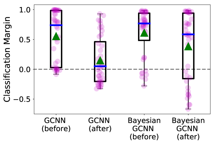
(a)

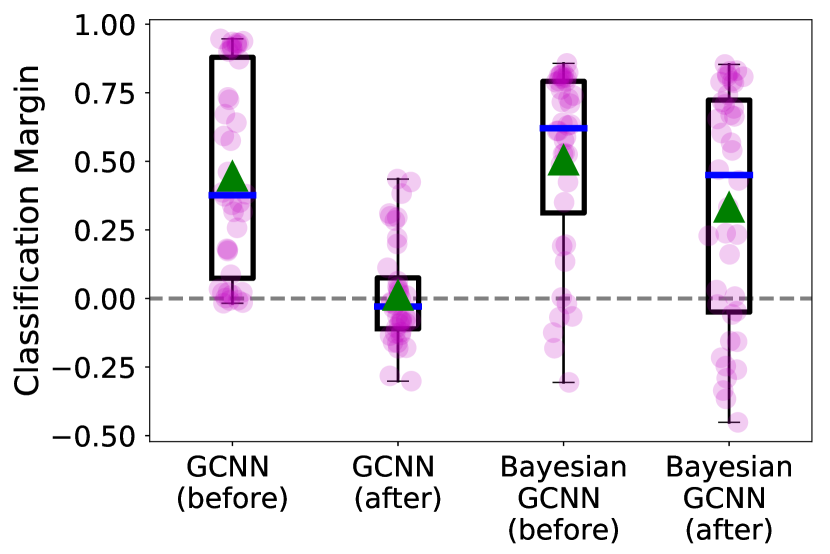
(b)

Figure 1: Boxplots of the average classification margin for 40 nodes before and after random attacks for GCNN and Bayesian GCNN on (a) Cora dataset and (b) Citeseer dataset. The box indicates 25-75 percentiles; the triangle represents the mean value; and the median is shown by a horizontal line. Whiskers extend to the minimum and maximum of data points.

6 Conclusions and Future Work

In this paper we have presented Bayesian graph convolutional neural networks, which provide an approach for incorporating uncertain graph information through a parametric random graph model. We provided an example of the framework for the case of an assortative mixed membership stochastic block model and explained how approximate inference can be performed using a combination of stochastic optimization (to obtain maximum a posteriori estimates of the random graph parameters) and approximate variational inference through Monte Carlo dropout (to sample weights from the Bayesian GCNN). We explored the performance of the Bayesian GCNN for the task of semi-supervised node classification and observed that the methodology improved upon state-of-the-art techniques, particularly for the case where the number of training labels is small. We also compared the robustness of Bayesian GCNNs and standard GCNNs under an adversarial attack involving randomly changing a subset of the edges of node. The Bayesian GCNN appears to be considerably more resilient to attack.

This paper represents a preliminary investigation into Bayesian graph convolutional neural networks and focuses on one type of graph model and one graph learning problem. In future work, we will expand the approach to other graph models and explore the suitability of the Bayesian framework for other learning tasks.

References

- [Airoldi et al. 2009] Airoldi, E. M.; Blei, D. M.; Fienberg, S. E.; and Xing, E. P. 2009. Mixed membership stochastic blockmodels. In Proc. Adv. Neural Inf. Proc. Systems, 33–40.
- [Anirudh and Thiagarajan 2017] Anirudh, R., and Thiagarajan, J. J. 2017. Bootstrapping graph convolutional neural networks for autism spectrum disorder classification. arXiv:1704.07487.
- [Atwood and Towsley 2016] Atwood, J., and Towsley, D. 2016. Diffusion-convolutional neural networks. In Proc. Adv. Neural Inf. Proc. Systems.
- [Bresson and Laurent 2017] Bresson, X., and Laurent, T. 2017. Residual gated graph convnets. arXiv:1711.07553.
- [Bruna et al. 2013] Bruna, J.; Zaremba, W.; Szlam, A.; and LeCun, Y. 2013. Spectral networks and locally connected networks on graphs. In Proc. Int. Conf. Learning Representations.
- [Chen, Ma, and Xiao 2018] Chen, J.; Ma, T.; and Xiao, C. 2018. FastGCN: fast learning with graph convolutional networks via importance sampling. In Proc. Int. Conf. Learning Representations (ICLR).
- [Defferrard, Bresson, and Vandergheynst 2016] Defferrard, M.; Bresson, X.; and Vandergheynst, P. 2016. Convolutional neural networks on graphs with fast localized spectral filtering. In Proc. Adv. Neural Inf. Proc. Systems.
- [Denker and Lecun 1991] Denker, J. S., and Lecun, Y. 1991. Transforming neural-net output levels to probability distributions. In Proc. Adv. Neural Inf. Proc. Systems.
- [Duvenaud, Maclaurin, and others 2015] Duvenaud, D.; Maclaurin, D.; et al. 2015. Convolutional networks on graphs for learning molecular fingerprints. In Proc. Adv. Neural Inf. Proc. Systems.
- [Frasconi, Gori, and Sperduti 1998] Frasconi, P.; Gori, M.; and Sperduti, A. 1998. A general framework for adaptive processing of data structures. IEEE Trans. Neural Networks 9(5):768–786.
- [Gal and Ghahramani 2016] Gal, Y., and Ghahramani, Z. 2016. Dropout as a Bayesian approximation: Representing model uncertainty in deep learning. In Proc. Int. Conf. Machine Learning.
- [Goodfellow, Shlens, and Szegedy 2015] Goodfellow, I.; Shlens, J.; and Szegedy, C. 2015. Explaining and harnessing adversarial examples. In Proc. Int. Conf. Learning Representations.
- [Gopalan, Gerrish, and others 2012] Gopalan, P. K.; Gerrish, S.; et al. 2012. Scalable inference of overlapping communities. In Proc. Adv. Neural Inf. Proc. Systems.
- [Hamilton, Ying, and Leskovec 2017] Hamilton, W.; Ying, R.; and Leskovec, J. 2017. Inductive representation learning on large graphs. In Proc. Adv. Neural Inf. Proc. Systems.
- [Henaff, Bruna, and LeCun 2015] Henaff, M.; Bruna, J.; and LeCun, Y. 2015. Deep convolutional networks on graph-structured data. arXiv:1506.05163.
- [Hernández-Lobato and Adams 2015] Hernández-Lobato, J. M., and Adams, R. 2015. Probabilistic backpropagation for scalable learning of Bayesian neural networks. In Proc. Int. Conf. Machine Learning.
- [Kipf and Welling 2017] Kipf, T., and Welling, M. 2017. Semi-supervised classification with graph convolutional networks. In Proc. Int. Conf. Learning Representations.
- [Korattikara et al. 2015] Korattikara, A.; Rathod, V.; Murphy, K.; and Welling, M. 2015. Bayesian dark knowledge. In Proc. Adv. Neural Inf. Proc. Systems.
- [Levie, Monti, and others 2017] Levie, R.; Monti, F.; et al. 2017. Cayleynets: Graph convolutional neural networks with complex rational spectral filters. arXiv:1705.07664.
- [Li, Ahn, and Welling 2016] Li, W.; Ahn, S.; and Welling, M. 2016. Scalable MCMC for mixed membership stochastic blockmodels. In Proc. Artificial Intelligence and Statistics, 723–731.
- [Li et al. 2016a] Li, C.; Chen, C.; Carlson, D.; and Carin, L. 2016a. Pre-conditioned stochastic gradient Langevin dynamics for deep neural networks. In Proc. AAAI Conf. Artificial Intelligence.
- [Li et al. 2016b] Li, Y.; Tarlow, D.; Brockschmidt, M.; and Zemel, R. 2016b. Gated graph sequence neural networks. In Proc. Int. Conf. Learning Rep. (ICLR).
- [Liao, Brockschmidt, and others 2018] Liao, R.; Brockschmidt, M.; et al. 2018. Graph partition neural networks for semi-supervised classification. arXiv preprint arXiv:1803.06272.
- [Louizos and Welling 2017] Louizos, C., and Welling, M. 2017. Multiplicative normalizing flows for variational Bayesian neural networks. arXiv:1703.01961.
- [MacKay 1992] MacKay, D. J. 1992. A practical Bayesian framework for backpropagation networks. Neural Comp. 4(3):448–472.
- [MacKay 1996] MacKay, D. J. C. 1996. Maximum entropy and Bayesian methods. Springer Netherlands. chapter Hyperparameters: Optimize, or Integrate Out?, 43–59.
- [Monti, Boscaini, and others 2017] Monti, F.; Boscaini, D.; et al. 2017. Geometric deep learning on graphs and manifolds using mixture model CNNs. In Proc. IEEE Conf. Comp. Vision and Pattern Recognition.
- [Monti, Shchur, and others 2018] Monti, F.; Shchur, O.; et al. 2018. Dual-primal graph convolutional networks. arXiv:1806.00770.
- [Neal 1993] Neal, R. M. 1993. Bayesian learning via stochastic dynamics. In Proc. Adv. Neural Inf. Proc. Systems, 475–482.
- [Patterson and Teh 2013] Patterson, S., and Teh, Y. W. 2013. Stochastic gradient Riemannian Langevin dynamics on the probability simplex. In Proc. Adv. Neural Inf. Proc. Systems.
- [Peixoto 2017] Peixoto, T. P. 2017. Bayesian stochastic blockmodeling. ArXiv e-print arXiv: 1705.10225.
- [Peng and Carvalho 2016] Peng, L., and Carvalho, L. 2016. Bayesian degree-corrected stochastic blockmodels for community detection. Electron. J. Statist. 10(2):2746–2779.
- [Scarselli, Gori, and others 2009] Scarselli, F.; Gori, M.; et al. 2009. The graph neural network model. IEEE Trans. Neural Networks 20(1):61–80.
- [Sen, Namata, and others 2008] Sen, P.; Namata, G.; et al. 2008. Collective classification in network data. AI Magazine 29(3):93.
- [Simonovsky and Komodakis 2017] Simonovsky, M., and Komodakis, N. 2017. Dynamic edge-conditioned filters in convolutional neural networks on graphs. arXiv:1704.02901.
- [Such, Sah, and others 2017] Such, F.; Sah, S.; et al. 2017. Robust spatial filtering with graph convolutional neural networks. IEEE J. Sel. Topics Signal Proc. 11(6):884–896.
- [Sukhbaatar, Szlam, and Fergus 2016] Sukhbaatar, S.; Szlam, A.; and Fergus, R. 2016. Learning multiagent communication with backpropagation. In Proc. Adv. Neural Inf. Proc. Systems, 2244–2252.
- [Sun, Chen, and Carin 2017] Sun, S.; Chen, C.; and Carin, L. 2017. Learning structured weight uncertainty in Bayesian neural networks. In Proc. Artificial Intelligence and Statistics.
- [Tishby, Levin, and Solla 1989] Tishby, N.; Levin, E.; and Solla, S. 1989. Consistent inference of probabilities in layered networks: Predictions and generalization. In Proc. Int. Joint Conf. Neural Networks.
- [Veličković et al. 2018] Veličković, P.; Cucurull, G.; Casanova, A.; Romero, A.; Liò, P.; and Bengio, Y. 2018. Graph attention networks. In Proc. Int. Conf. Learning Representations.
- [Yang, Cohen, and Salakhutdinov 2016] Yang, Z.; Cohen, W. W.; and Salakhutdinov, R. 2016. Revisiting semi-supervised learning with graph embeddings. arXiv preprint arXiv:1603.08861.
- [Zügner, Akbarnejad, and Günnemann 2018] Zügner, D.; Akbarnejad, A.; and Günnemann, S. 2018. Adversarial attacks on neural networks for graph data. In Proc. ACM Int. Conf. Knowl. Disc. Data Mining.