Caching to the Sky: Performance Analysis of Cache-Assisted CoMP for Cellular-Connected UAVs

Abstract

Providing connectivity to aerial users, such as cellular-connected unmanned aerial vehicles (UAVs) or flying taxis, is a key challenge for tomorrow’s cellular systems. In this paper, the use of coordinated multi-point (CoMP) transmission along with caching for providing seamless connectivity to aerial users is investigated. In particular, a network of clustered cache-enabled small base stations (SBSs) serving aerial users is considered in which a requested content by an aerial user is cooperatively transmitted from collaborative ground SBSs. For this network, a novel upper bound expression on the coverage probability is derived as a function of the system parameters. The effects of various system parameters such as collaboration distance and content availability on the achievable performance are then investigated. Results reveal that, when the antennas of the SBSs are tilted downwards, the coverage probability of a high-altitude aerial user is upper bounded by that of a ground user regardless of the transmission scheme. Moreover, it is shown that for a low signal-to-interference-ratio (SIR) threshold, CoMP transmission improves the coverage probability for aerial users from $10\%$ to $70\%$ under a collaboration distance of $200\text{\,}\mathrm{m}$.

I Introduction

The past few years have witnessed a tremendous increase in the use of unmanned aerial vehicles (UAVs), also known as drones, in many applications, such as aerial surveillance, package delivery, and even flying taxis [1]. Enabling such UAV-centric applications requires ubiquitous wireless connectivity that can be potentially provided by the popular wireless cellular network [2, 3, 4]. However, in order to operate such cellular-connected UAVs using existing wireless systems, one must address a broad range of challenges that include resource management, interference mitigation, power control, and energy efficiency [5].

In particular, the altitude of a cellular-connected UAV will be much higher than the typical terrestrial user equipment (UE) and will significantly exceed the small base station (SBS) antenna height. Consequently, ground SBSs need to be able to provide 3D communication coverage. However, existing SBSs antennas are usually tilted downwards to cater to the ground coverage and reduce inter-cell interference. Preliminary field measurement results by Qualcomm have demonstrated adequate aerial coverage by SBS antenna sidelobes for UAVs below $120\text{\,}\mathrm{m}$ [6]. However, as the UAV altitude further increases, new solutions are needed to enable cellular SBSs to seamlessly cover the sky [7, 8].

The dominance of line-of-sight (LoS) links makes inter-cell interference a critical issue for cellular systems with hybrid terrestrial and aerial UEs. In this regard, extensive real-world simulations and fields trials in [5, 9], and [10] have shown that an aerial UE, in general, has poorer downlink performance than a ground UE. Due to the down-tilted SBS antennas, it is found that UAVs at $40\text{\,}\mathrm{m}$ and higher are served by the sidelobes of SBS antennas, which have reduced antenna gain compared to the mainlobes of SBS antennas serving ground UEs. However, UEs at $40\text{\,}\mathrm{m}$ and above experience free space propagation conditions, while radio signals attenuate more quickly with distance on the ground. Interestingly, it is shown that free space propagation can make up for the SBS antenna sidelobe gain reduction [9]. However, this merit from such a favorable LoS channel vanishes at high altitudes because the free space propagation also leads to stronger LoS interfering signals. Eventually, aerial UEs at high altitudes are shown to always have poorer communication and coverage as opposed to ground UEs [9, 5], and [10]. Nevertheless, while interesting, these works explored the feasibility of providing cellular connectivity for UAVs without proposing new approaches to solve the ensuing LoS-dominated interference problem.

In [8], the authors studied the feasibility of supporting drone operations using existent cellular infrastructure. The authors showed that carefully designed system parameters such as antenna radiation pattern and network density guarantee a satisfactory quality of service. Meanwhile, the authors in [11] considered a cellular-connected UAV flying from an initial location to a final destination. The authors minimized the UAV’s mission completion time by optimizing its trajectory while maintaining reliable communication with the ground cellular network. However, while the works in [7, 8], and [11] have analyzed the performance of cellular-connected UAVs, effectively mitigating the impact of LoS interference on contemporary aerial UEs has not yet been addressed in the literature.

Compared with this prior art [5, 6, 7, 8, 9, 10, 11], the main contribution of this paper is to develop a novel framework that leverages coordinated multi-point (CoMP) transmissions for serving high-altitude cellular-connected UAVs while mitigating cross-cell interference and boosting the received signal-to-interference-ratio (SIR). In particular, we consider a network of cache-enabled SBSs in which an aerial UE downloads a previously cached content via CoMP transmission from neighboring ground SBSs. Using tools from stochastic geometry, we derive a considerably tight upper bound on the content coverage probability as a function of the system parameters. We show that the achievable performance of an aerial user depends heavily on the collaboration distance, content availability, and target bit rate. Moreover, while allowing CoMP transmission substantially improves the coverage probability for aerial UEs, it is shown that their performance is still upper bounded by that of ground UEs due to the down-tilt of the current SBSs’ antennas. To the best of our knowledge, this paper provides the first analysis of CoMP transmission for cellular-connected UAVs in cache-enabled networks.

The rest of this paper is organized as follows. Section II and Section III present the system model and the coverage probability analysis, respectively. Numerical results are presented in Section IV and conclusions are drawn in Section V.

II System Model

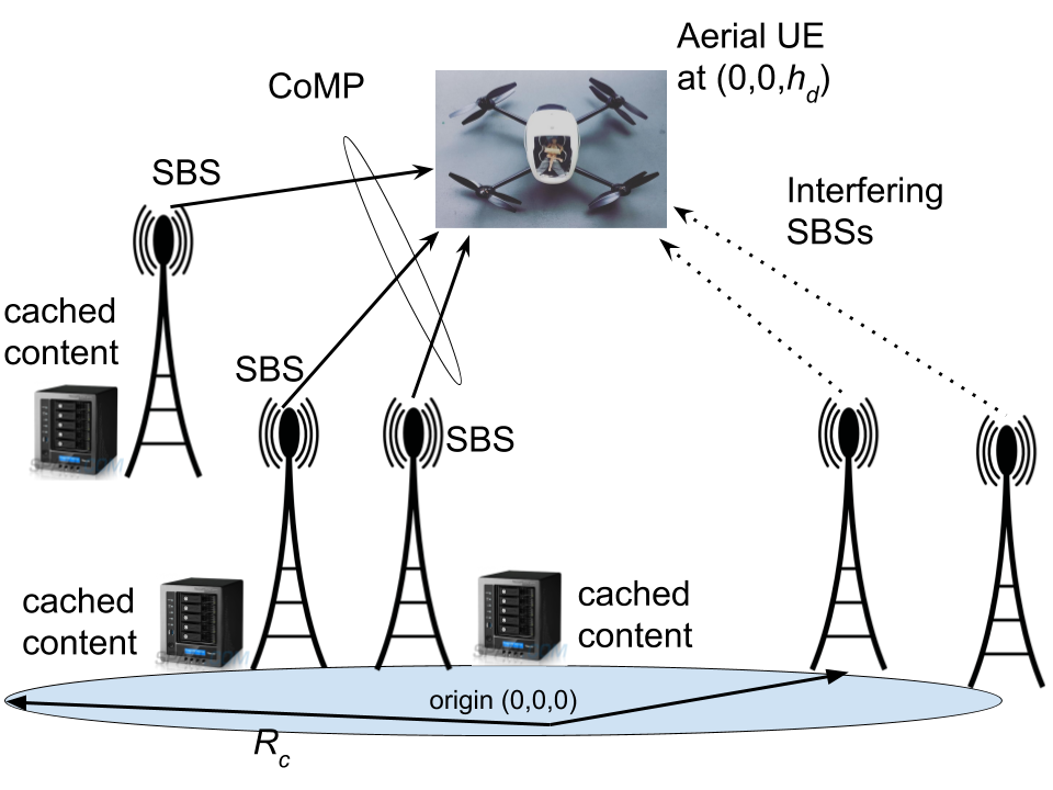
Figure 1: Illustration of the proposed system model.

We consider a cache-enabled small cell network in which SBSs are distributed according to a homogeneous Poisson point process (PPP) $\Phi_{b}=\{b_{i}\in\mathbb{R}^{2},\forall i\in\mathbb{N}^{+}\}$ with intensity $\lambda_{b}$. We consider a cellular-connected aerial UE flying at an altitude $h_{d}$ and located at $(0,0,h_{d})\in\mathbb{R}^{3}$, where $h_{d}$ is the altitude of the UAV. We assume a user-centric model in which the SBSs are grouped into disjoint clusters around aerial UEs to be served [12]. A cluster is represented by a circle of radius $R_{c}$ centered at the terrestrial projection of an aerial UE, as shown in Fig. 1. The area of each cluster is then given by $A=\pi R_{c}^{2}$.

SBSs belonging to the same cluster can cooperate to serve cached content to the aerial UE whose projection on the ground is assumed at the cluster center. The aerial UE can represent a conventional cellular-connected UAV or a passenger of a flying drone-taxi [1]. Due to the strong LoS-dominated interference at high altitudes, we allow multiple SBSs within a certain distance from the aerial UE to cooperatively transmit a requested content that they previously cached.

II-A Probabilistic Caching Placement

Each SBS has a surplus memory designated for caching content from a known file library. These files represent the content catalog that an aerial UE may request, and are indexed in a descending order of popularity. We adopt a random content placement policy in which each content $f$ is cached independently at each SBS according to a probability $c_{f}$, $0\leq c_{f}\leq 1$. Note that SBSs caching content $f$ can be modeled as a PPP $\Phi_{bf}$ with the intensity function given by the independent thinning theorem as $\lambda_{bf}=c_{f}\lambda_{b}$ [13]. Similarly, SBSs not caching a content $f$ can be modeled as another PPP $\Phi_{bf}^{!}$ with intensity function $\lambda_{bf}^{\circ}=(1-c_{f})\lambda_{b}$, where $\Phi_{b}=\Phi_{bf}\cup\Phi_{bf}^{!}$. The probability mass function (PMF) of the number of SBSs caching content $f$ in a cluster is given by:

$$\mathbb{P}(n=\kappa)=\frac{(c_{f}\lambda_{b}A)^{\kappa}e^{-c_{f}\lambda_{b}A}}{\kappa!},$$ (1)

which represents a Poisson distribution with mean $c_{f}\lambda_{b}A$.

II-B Serving Distance Distributions

Under the condition of having $\kappa$ caching SBSs in the cluster of interest, the distribution of such in-cluster caching SBSs will follow a binomial point process (BPP). This BPP consists of $\kappa$ uniformly and independently distributed SBSs in the cluster.

The set of cooperative SBSs providing content $f$ is defined as $\Phi_{cf}=\{b_{i}\in\Phi_{bf}\cap\mathcal{B}(0,R_{c})\}$, where $\mathcal{B}(0,R_{c})$ denotes the ball centered at the origin with radius $R_{c}$. Considering the aerial UE located at the origin in $\mathbb{R}^{2}$, i.e., $(0,0,h_{d})\in\mathbb{R}^{3}$, the 2D distances from the cooperative SBSs to the aerial UE are denoted by $\boldsymbol{R}_{\kappa}=[R_{1},\dots,R_{\kappa}]$. Then, conditioning on $\boldsymbol{R}_{\kappa}=\boldsymbol{r}_{\kappa}$, where $\boldsymbol{r}_{\kappa}=[r_{1},\dots,r_{\kappa}]$, the conditional probability distribution function (PDF) of the joint serving distances’ distribution is denoted as $f_{\boldsymbol{R}_{\kappa}}(\boldsymbol{r}_{\kappa})$. The $\kappa$ cooperative SBSs that cache a content $f$ can be seen as the $\kappa$-closest SBSs to the cluster center from the PPP $\Phi_{bf}$. Since the $\kappa$ SBSs are independently and uniformly distributed in the cluster approximated by $\mathcal{B}(0,R_{c})$, we have the PDF of the horizontal distance $r_{i}$ from SBS $i$ to the aerial UE at $(0,0,h_{d})$ given as [13]

$$f_{R_{i}}(r_{i})=\left\{\begin{array}[]{ll}\frac{2r_{i}}{R_{c}^{2}},\quad\quad\quad 0\leq r_{i}\leq R_{c},\\ 0,\quad\quad\quad\quad{\rm otherwise},\end{array}\right.$$

for any $i\in\mathcal{K}_{f}=\{1,\dots,\kappa\}$, where $\mathcal{K}_{f}$ is the set of SBSs that cache a content $f$ within the ball $\mathcal{B}(0,R_{c})$. From the i.i.d. property of BPP, the conditional joint PDF of the serving distances $\boldsymbol{R}_{\kappa}=[R_{1},\dots,R_{\kappa}]$ is

$$f_{\boldsymbol{R}_{\kappa}}(\boldsymbol{r}_{\kappa})=\prod_{i=0}^{\kappa}\frac{2r_{i}}{R_{c}^{2}}.$$ (2)

We consider a content delivery from ground SBSs having the same height $h_{\textrm{SBS}}$ to an aerial UE located at altitude $h_{d}$. The SBS vertical antenna pattern is directional and down-tilted for ground UEs. The vertical antenna beamwidth and down-tilt angle of the SBSs are denoted respectively by $\theta_{B}$ and $\theta_{t}$. The side and main lobe gains of the antennas are denoted by $G_{s}$ and $G_{m}$, respectively. Since the horizontal distance between the aerial UE and SBS $i$ is $r_{i}$, the communication link distance will be $d_{i}=\sqrt{r_{i}^{2}+(h_{d}-h_{\textrm{SBS}})^{2}}$ for all $i\in\mathcal{K}_{f}$.

II-C Channel Model

For the CoMP transmission between SBSs and the aerial UE, we consider a wireless channel that is characterized by both large-scale and small-scale fading. For the large-scale fading, the channel between SBS $i$ and the aerial user is described by the LoS and non-line-of-sight (NLoS) components, which are considered separately along with their probabilities of occurrence [14]. This assumption is apropos for such ground-to-air channels that are often dominated by LoS communication [7]. Therefore, the antenna gain plus path loss for each component, i.e., LoS and NLoS, will be

$$\zeta_{v}(r_{i})=A_{v}G(r_{i})d_{i}^{-\alpha_{v}}=A_{v}G(r_{i})\big{(}r_{i}^{2}+(h_{d}-h_{\textrm{SBS}})^{2}\big{)}^{-\alpha_{v}/2},$$ (3)

where $v\in\{l,n\}$, $\alpha_{l}$ and $\alpha_{n}$ are the path loss exponents for the LoS and NLoS links, respectively, with $\alpha_{l}<\alpha_{n}$, and $A_{l}$ and $A_{n}$ are the path-loss constants at the reference distance $d_{i}=$1\text{\,}\mathrm{m}$$ for the LoS and NLoS, respectively. $G(r_{i})$ is the total antenna directivity gain between SBS $i$ and the aerial UE, which can be written similar to [8] as

$$G(r_{i})=\left\{\begin{array}[]{ll}G_{m},\quad\quad\quad{\rm for\quad}r_{i}\in\mathcal{S}_{bs},\\ G_{s},\quad\quad\quad{\rm for\quad}r_{i}\notin\mathcal{S}_{bs},\end{array}\right.$$

where $\mathcal{S}_{bs}$ is formed by all the distances $r_{i}$ satisfying $h_{\textrm{SBS}}-r_{i}{\rm tan}(\theta_{t}+\frac{\theta_{B}}{2})<h_{d}<h_{\textrm{SBS}}-r_{i}{\rm tan}(\theta_{t}-\frac{\theta_{B}}{2})$. In other words, the horizontal distance between a SBS and an aerial UE along with the antenna height, antenna beamwidth and down-tilt angles, and the altitude of this aerial UE determine whether it is served by a mainlobe or sidelobe of a SBS antenna.

For the small-scale fading, we adopt a Nakagami-$m$ model utilized in [7] and [8] for the channel gain, whose PDF is given by:

$$f(\omega)=\frac{2\frac{m}{\eta}^{m}\omega^{2m-1}}{\Gamma(m)}{\rm exp}\big{(}-\frac{m}{\eta}\omega^{2}\big{)},$$ (4)

where $\eta$ is a controlling spread parameter, and the fading parameter $m$ is assumed to be an integer for analytical tractability. Since the communication links between an aerial UE and SBSs are LoS-dominated, e.g., suburban environments with $h_{d}>$40\text{\,}\mathrm{m}$$ [9], it is assumed to have $m>1$. Given that $\omega\sim$ Nakagami$(m,\eta/m)$, it directly follows that the channel gain power $\gamma=\omega^{2}\sim\Gamma(m,\eta/m)$, where $\Gamma(k,\theta)$ is a Gamma random variable (RV) with $k$ and $\theta$ denoting the shape and scale parameters, respectively. Hence, the PDF of channel power gain distribution will be:

$$f(\gamma)=\frac{(\frac{m}{\eta})^{m}\gamma^{m-1}}{\Gamma(m)}{\rm exp}\big{(}-\frac{m}{\eta}\gamma\big{)}.$$ (5)

3D blockage is characterized by the fraction $a$ of the total land area occupied by buildings, the mean number of buildings $e$ per $\text{\,}\mathrm{k}\mathrm{m}$², and the buildings height modeled by a Rayleigh PDF with a scale parameter $c$. Hence, the probability of LoS of a caching SBS at a distance $r_{i}$ from the aerial UE is given by [15]:

$$\mathbb{P}_{l}(r_{i})=\prod_{n=0}^{{\rm max}(p-1,0)}\Bigg{[}1-{\rm exp}\Big{(}-\frac{\big{(}h_{\textrm{SBS}}+\frac{h(n+0.5)}{m+1}\big{)}^{2}}{2c^{2}}\Big{)}\Bigg{]},$$ (6)

where $h=h_{d}-h_{\textrm{SBS}}$ and $p=\lfloor\frac{r_{i}\sqrt{ae}}{1000}\rfloor$. Different terrain structures and environments can be considered by by varying the set of $(a,e,c)$.

As discussed previously, the performance of a high-altitude aerial UE is limited by the LoS interference they encounter. We hence propose a multi-SBSs cooperative transmission scheme aiming at mitigating inter-cell interference and improving the performance of such high-altitude aerial UEs. Under this setting, in the next section we develop a novel mathematical framework to characterize the performance of cache-assisted CoMP transmission for cellular-connected UAVs. The performance of UAVs is then contrasted to their terrestrial counterparts.

III Coverage Probability Analysis

In this section, we characterize the network performance in terms of coverage probability. We assume that the SBSs have the same transmit power $P_{t}$. Without loss of generality, we consider a typical aerial UE located at $(0,0,h_{d})\in\mathbb{R}^{3}$. Conditioning on having $\kappa$ SBSs serving a content $f$, the received signal at the aerial UE will be:

$$P =\underbrace{\sum_{i=1}^{\kappa}P(r_{i})\omega_{i}w_{i}X_{f}}_{\text{desired signal}}+\underbrace{\sum_{j\in\Phi_{bf}^{!}\cap\mathcal{B}(0,R_{c})}P(u_{j})\omega_{j}w_{j}Y_{j}}_{I_{\text{in}}}$$

$$+\underbrace{\sum_{k\in\Phi_{b}\setminus\mathcal{B}(0,R_{c})}P(u_{k})\omega_{k}w_{k}Y_{k}}_{I_{\text{out}}}+\quad Z,$$ (7)

where the first term represents the desired signal from $\kappa$ transmitting SBSs with $P(r_{i})=\sqrt{P_{t}}\zeta_{v}(r_{i})^{0.5}$, $v\in\{l,n\}$, $\omega_{i}$ being the Nakagami-$m$ fading variable of the channel from SBS $i$ to the aerial UE, $w_{i}$ is the precoder used by SBS $i$, and $X_{f}$ is the channel input symbol that is sent by the cooperating SBSs. The second and third terms represent the in-cluster interference $I_{\text{in}}$, and the out-of-cluster interference $I_{\text{out}}$, respectively. $Y_{j}$ is the transmitted symbol from interfering SBS $j$ and

$$P(u_{j})=\left\{\begin{array}[]{ll}P_{l}(u_{j})=\sqrt{P_{t}}\zeta_{l}(u_{j})^{0.5},\quad\quad\quad{\rm for\quad LoS},\\ P_{n}(u_{j})=\sqrt{P_{t}}\zeta_{n}(u_{j})^{0.5},\quad\quad\quad{\rm for\quad NLoS},\end{array}\right.$$

where $u_{j}$ is the horizontal distance between interfering SBS $j$ and the aerial UE. $Z$ is a circular-symmetric zero-mean complex Gaussian RV modeling the background thermal noise. In-cluster interference occurs only for the case in which not all of the collaborative SBSs (within distance $R_{c}$) have the cached content (i.e., $c_{f}<1$). In this case, the set of interfering SBSs will be characterized by $\Phi_{b}\setminus\Phi_{cf}=\Big{\{}b_{i}\in\big{\{}\Phi_{b}\setminus\mathcal{B}(0,R_{c})\big{\}}\cup\big{\{}\Phi_{bf}^{!}\cap\mathcal{B}(0,R_{c})\big{\}}\Big{\}}$. For ease of notation, we denote $\big{\{}\Phi_{bf}^{!}\cap\mathcal{B}(0,R_{c})\big{\}}$ as $\Phi_{cf}^{!}$. Otherwise, for $c_{f}=1$, there is no in-cluster interference and the set of interfering SBSs will then be $\Phi_{b}\setminus\Phi_{cf}=\{b_{i}\in\Phi_{b}\setminus\mathcal{B}(0,R_{c})\}$.

We assume that the channel state information (CSI) is available at the serving SBSs, i.e., the precoder $w_{i}$ can be set as $\frac{\omega_{i}^{*}}{|\omega_{i}|}$, where $\omega_{i}^{*}$ is the complex conjugate of $\omega_{i}$. Assuming that $X_{f}$, $Y_{j}$, and $Y_{k}$ in (III) are independent zero-mean RVs of unit variance, and averaging over all LoS and NLoS configurations for the $\kappa$ caching SBSs, the SIR at the aerial UE will then be:

$$\Upsilon_{|\boldsymbol{r}_{\kappa}} =\sum_{o=0}^{\kappa}{\kappa\choose o}\prod_{i=0}^{o}\mathbb{P}_{l}(r_{i})\prod_{j=o+1}^{\kappa}\mathbb{P}_{n}(r_{j})\cdot$$

$$\frac{P_{t}\Bigg{|}\sum_{i=1}^{o}\zeta_{l}^{1/2}(r_{i})\omega_{i}+\sum_{j=o+1}^{\kappa}\zeta_{n}^{1/2}(r_{j})\omega_{j}\Bigg{|}^{2}}{I_{\text{in}}+I_{\text{out}}}.$$ (8)

In (III), we have $\big{|}\sum_{i=1}^{o}\zeta_{l}^{1/2}(r_{i})\omega_{i}+\sum_{j=o+1}^{\kappa}\zeta_{n}^{1/2}(r_{j})\omega_{j}\big{|}^{2}$ representing the square of a weighted sum of $\kappa$ Nakagami-$m$ RVs. Since there is no known closed-form expression for a weighted sum of Nakagami-$m$ RVs, we use the Cauchy-Schwarz’s inequality to get an upper bound on a square of weighted sum as follows:

$$\Bigg{|}\sum_{i=1}^{o}\zeta_{l}^{1/2}(r_{i})\omega_{i}+ \sum_{j=o+1}^{\kappa}\zeta_{n}^{1/2}(r_{j})\omega_{j}\Bigg{|}^{2}=\Bigg{(}\sum_{i=1}^{\kappa}Q_{i}\Bigg{)}^{2}$$

$$\leq\kappa\Bigg{(}\sum_{i=1}^{\kappa}Q_{i}^{2}\Bigg{)},$$ (9)

where $Q_{i}=\zeta_{v}^{1/2}(r_{i})\omega_{i}$, is a scaled Nakagami-$m$ RV, with $v\in\{l,n\}$ and $i\in\mathcal{K}_{f}$. Since $\omega_{i}\sim$ Nakagami$(m,\eta/m)$, from the scaling property of the Gamma PDF, $Q_{i}^{2}\sim\Gamma\big{(}k_{i}=m,\theta_{i}=2\eta\zeta_{v}(r_{i})/m\big{)}$. To get a statistical equivalent PDF of a sum of $\kappa$ Gamma RVs $Q_{i}$ with different shape parameters $\theta_{i}$, we adopt the method of sum of Gammas second-order moment match proposed in [16, Proposition 8]. It is shown that the equivalent Gamma distribution, denoted as $J\sim\Gamma(k,\theta)$, with the same first and second-order moments has the parameters $k=\Big{(}\sum_{i}{k_{i}\theta_{i}}\Big{)}^{2}/\sum_{i}{k_{i}\theta_{i}^{2}}$ and $\theta=\sum_{i}{k_{i}\theta_{i}^{2}}/\sum_{i}k_{i}\theta_{i}$. To showcase the accuracy of the second-order moment approximation in our case, for an arbitrary realization of the network, we plot in Fig. 2 the PDF of the equivalent channel gain. As evident from the plot, approximating a sum of $\kappa$ Gamma RVs with an equivalent Gamma RV whose parameters are

$$k=\frac{m\big{(}\sum_{i}{\zeta_{v}(r_{i})}\big{)}^{2}}{\sum_{i}{\big{(}\zeta_{v}(r_{i})\big{)}^{2}}}\quad\quad\text{and}\quad\quad\theta=\frac{\eta\sum_{i}{\zeta_{v}(r_{i})}}{m\sum_{i}\zeta_{v}(r_{i})},$$ (10)

is quite accurate. For tractability, we further upper bound the shape parameter $k$ in (10):

$$k=m\frac{\Big{(}\sum_{i}\zeta_{v}(r_{i})\Big{)}^{2}}{\sum_{i}\Big{(}\zeta_{v}(r_{i})\Big{)}^{2}}\leq m\frac{\kappa\sum_{i}\Big{(}\zeta_{v}(r_{i})\Big{)}^{2}}{\sum_{i}\Big{(}\zeta_{v}(r_{i})\Big{)}^{2}}=m\kappa,$$ (11)

where $m\kappa$ is integer.

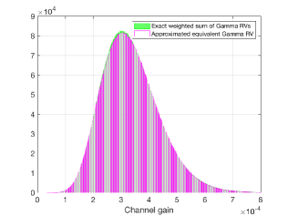
Figure 2: Monte Carlo simulation of the PDF of the equivalent gain of channels between cooperating SBSs and the aerial UE, including path loss and fading. A PPP realization of density $\lambda_{b}=20$ SBS/$\text{\,}\mathrm{k}\mathrm{m}$² is run for a simulated area of $20\text{\,}\mathrm{k}\mathrm{m}$² with $m=3$ and $R_{c}=$200\text{\,}\mathrm{m}$$.

We next derive an upper bound expression on the coverage probability. The novelty of our approach is that it adopts an upper bound on the square of summed Nakagami-$m$ RVs and second-order match approximation of Gamma RVs. This allows us to get a closed-form upper bound on the coverage probability, which is difficult to obtain exactly.

The coverage probability of the aerial UE conditioned on the serving distances $\boldsymbol{r}_{\kappa}$ is then expressed as

$$\mathbb{P}_{\textrm{cov}|\boldsymbol{r}_{\kappa}}=\mathbb{P}\big{[}\Upsilon_{|\boldsymbol{r}_{\kappa}}>\vartheta\big{]}$$ (12)

$$\approx\sum_{o=0}^{\kappa}{\kappa\choose o}\prod_{i=0}^{o}\mathbb{P}_{l}(r_{i})\prod_{j=o+1}^{\kappa}\mathbb{P}_{n}(r_{j})\mathbb{P}\Big{(}\frac{\kappa P_{t}\big{(}\sum_{i=1}^{\kappa}Q_{i}\big{)}^{2}}{I_{\text{in}}+I_{\text{out}}}>\vartheta\Big{)},$$

$$=\sum_{o=0}^{\kappa}{\kappa\choose o}\prod_{i=0}^{o}\mathbb{P}_{l}(r_{i})\prod_{j=o+1}^{\kappa}\mathbb{P}_{n}(r_{j})\mathbb{P}\Big{(}\frac{\kappa P_{t}J}{I_{\text{in}}+I_{\text{out}}}>\vartheta\Big{)},$$ (13)

where $\vartheta$ is the $\mathrm{SIR}$ threshold. The unconditional coverage probability can be obtained as a function of the system parameters, as stated formally in the following theorem.

Theorem 1.

The coverage probability is given by:

$$\mathbb{P}_{{\rm cov}}=\sum_{\kappa=1}^{\infty}\mathbb{P}(n=\kappa)\int_{\boldsymbol{r_{\kappa}}=\boldsymbol{0}}^{\boldsymbol{R_{c}}}\mathbb{P}_{{\rm cov}|\boldsymbol{r}_{\kappa}}\prod_{i=0}^{\kappa}\frac{2r_{i}}{R_{c}^{2}}\differential{\boldsymbol{r}_{\kappa}},$$ (14)

where $\mathbb{P}_{{\rm cov}|\boldsymbol{r}_{\kappa}}$ is the conditional coverage probability in (16) (at the top of next page), where $\varpi=\vartheta/\kappa P_{t}\theta$.

Proof.

We proceed to obtain the coverage probability as follows:

$$\mathbb{P}\Big{(}\frac{\kappa P_{t}J}{I_{\text{in}}+I_{\text{out}}}>\vartheta\Big{)}=\mathbb{P}\Big{(}\kappa P_{t}J>\vartheta\big{(}I_{\text{in}}+I_{\text{out}}\big{)}\Big{)}$$

$$=\mathbb{E}_{I_{\text{in}},I_{\text{out}}}\Bigg{[}\mathbb{P}\Big{(}\kappa P_{t}J>\vartheta\big{(}I_{\text{in}}+I_{\text{out}}\big{)}\Big{)}\Bigg{]}$$

$$=\mathbb{E}_{I_{\text{in}},I_{\text{out}}}\Bigg{[}\mathbb{P}\Big{(}J>\frac{\vartheta}{\kappa P_{t}}\big{(}I_{\text{in}}+I_{\text{out}}\big{)}\Big{)}\Bigg{]}$$

$$\overset{(a)}{\approx}\mathbb{E}_{I_{\text{in}},I_{\text{out}}}\Big{[}\sum_{k=0}^{k-1}\frac{(\vartheta/\kappa P_{t}\theta)^{k}}{k!}\big{(}I_{\text{in}}+I_{\text{out}}\big{)}^{k}{\rm exp}\Big{(}-\frac{\vartheta}{\kappa P_{t}\theta}\big{(}I_{\text{in}}+I_{\text{out}}\big{)}\Big{)}\Big{]}$$

$$\overset{(b)}{=}\mathbb{E}_{I_{\text{in}},I_{\text{out}}}\Big{[}\sum_{k=0}^{k-1}\frac{(-\varpi)^{k}}{k!}\frac{d^{k}}{d\vartheta^{k}}\mathcal{L}_{I_{\text{in}}+I_{\text{out}}|\boldsymbol{r}_{\kappa}}(\varpi)\Big{]},$$ (15)

where (a) follows from the PDF of Gamma RV $J$ with parameters $\theta$ and $k$ given in (10) and (11), respectively. (b) follows from the fact that $\varpi=\vartheta/\kappa P_{t}\theta$ along with the Laplace transform definition of the RV $I_{\text{in}}+I_{\text{out}}$. Next, we derive the Laplace transform of interference:

$$\mathbb{P}_{\textrm{cov}|\boldsymbol{r}_{\kappa}}=\sum_{o=0}^{\kappa}{\kappa\choose o}\prod_{i=0}^{o}\mathbb{P}_{l}(r_{i})\prod_{i=o+1}^{\kappa}\mathbb{P}_{n}(r_{i})\sum_{k=0}^{k-1}\frac{(-\varpi)^{k}}{k!}\frac{\partial^{k}}{\partial\varpi^{k}}\cdot$$

$${\rm exp}\Bigg{(}-2\pi\lambda_{bf}^{\circ}\int_{v=0}^{R_{c}}\Big{(}1-\delta_{l}\mathbb{P}_{l}(v)-\delta_{n}\mathbb{P}_{n}(v)\Big{)}v\differential{v}\Bigg{)}{\rm exp}\Bigg{(}-2\pi\lambda_{p}\int_{v=R_{c}}^{\infty}\Big{(}1-\delta_{l}\mathbb{P}_{l}(v)-\delta_{n}\mathbb{P}_{n}(v)\Big{)}v\differential{v}\Bigg{)}.$$ (16)

$$\mathcal{L}_{I_{\text{in}}+I_{\text{out}}|\boldsymbol{r}_{\kappa}}(\varpi)=\mathbb{E}_{I_{\text{in}},I_{\text{out}}}\Big{[}{\rm exp}\big{(}-\varpi(I_{\text{in}}+I_{\text{out}})\big{)}\Big{]}$$

$$=\mathbb{E}\Bigg{[}e^{-\varpi\sum_{j\in\Phi_{cf}^{!}}\gamma_{j}P(u_{j})^{2}}e^{-\varpi\sum_{j\in\Phi_{b}\setminus\mathcal{B}(0,R_{c})}\gamma_{j}P(u_{j})^{2}}\Bigg{]}$$

$$=\mathbb{E}_{\Phi_{b}}\Big{[}\prod_{j\in\Phi_{cf}^{!}}\mathbb{E}_{\gamma_{j}}e^{-\varpi\gamma_{j}P(u_{j})^{2}}\prod_{j\in\Phi_{b}\setminus\mathcal{B}(0,R_{c})}\mathbb{E}_{\gamma_{j}}e^{-\varpi\gamma_{j}P(u_{j})^{2}}\Big{]}$$

$$\overset{(a)}{=}\mathbb{E}_{\Phi_{b}}\Bigg{[}\prod_{j\in\Phi_{cf}^{!}}\Big{[}\Big{(}1+\frac{\varpi P_{l}(u_{j})^{2}}{m}\Big{)}^{-m}\mathbb{P}_{l}(u_{j})+$$

$$\Big{(}1+\frac{\varpi P_{n}(u_{j})^{2}}{m}\Big{)}^{-m}\mathbb{P}_{n}(u_{j})\Big{]}\cdot$$

$$\prod_{j\in\Phi_{b}\setminus\mathcal{B}(0,R_{c})}\Big{[}\Big{(}1+\frac{\varpi P_{l}(u_{j})^{2}}{m}\Big{)}^{-m}$$

$$\cdot\mathbb{P}_{l}(u_{j})+\Big{(}1+\frac{\varpi P_{n}(u_{j})^{2}}{m}\Big{)}^{-m}\mathbb{P}_{n}(u_{j})\Big{]}\Bigg{]}$$

$$\overset{(b)}{=}{\rm exp}\Bigg{(}-2\pi\lambda_{bf}^{\circ}\int_{v=0}^{R_{c}}\Big{(}1-\delta_{l}\mathbb{P}_{l}(v)-\delta_{n}\mathbb{P}_{n}(v)\Big{)}v\differential{v}\Bigg{)}\cdot$$

$${\rm exp}\Bigg{(}-2\pi\lambda_{p}\int_{v=R_{c}}^{\infty}\Big{(}1-\delta_{l}\mathbb{P}_{l}(v)-\delta_{n}\mathbb{P}_{n}(v)\Big{)}v\differential{v}\Bigg{)},$$ (17)

where (a) follows from the moment generating function (MGF) of gamma distribution. (b) follows from the probability generating functional (PGFL) of PPP, the substitution $\delta_{l}=\big{(}1+\frac{\varpi P_{l}(v)^{2}}{m}\big{)}^{-m}$ and $\delta_{n}=\big{(}1+\frac{\varpi P_{n}(v)^{2}}{m}\big{)}^{-m}$, and Cartesian to polar coordinates conversion. By using (13), (15), and (III) along with the PMF of the number of caching SBSs given in (1), the coverage probability is obtained. ∎

Important insights about the coverage probability can be obtained from (14). First, if the collaboration distance $R_{c}$ or the caching probability $c_{f}$ increases, both the probability $\mathbb{P}(n=\kappa)$ and the integrand value in (14) increase, and, thus, the coverage probability grows accordingly. Furthermore, the effect of the spatial SBS density $\lambda_{b}$ on the coverage probability is two-fold. On the one hand, the average number of caching SBSs increases with $\lambda_{b}$ as characterized by $\mathbb{P}(n=\kappa)$, which results in a higher desired signal power. On the other hand, this advantage is counter-balanced by the increase in interference power when $\lambda_{b}$ increases, as captured in the decaying exponential functions in (16).

IV Numerical Results

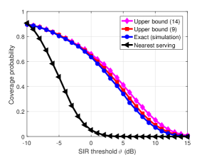
Figure 3: The derived upper bound on the coverage probability is plotted versus the SIR threshold $\vartheta$.

TABLE I: Simulation Parameters

Description	Parameter	Value
LoS path-loss exponent	$\alpha_{l}$	2.09
NLoS path-loss exponent	$\alpha_{n}$	3.75
LoS path-loss constant	$A_{l}$	$-41.1\text{\,}\mathrm{d}\mathrm{B}$
NLoS path-loss constant	$A_{n}$	$-32.9\text{\,}\mathrm{d}\mathrm{B}$
Antenna main lobe gain	$G_{m}$	$10\text{\,}\mathrm{d}\mathrm{B}$
Antenna side lobe gain	$G_{s}$	$-3.01\text{\,}\mathrm{d}\mathrm{B}$
Nakagami fading parameter	$m$	3
Nakagami spreading factor	$\eta$	2
SBS antenna height	$h_{\textrm{SBS}}$	$30\text{\,}\mathrm{m}$
Aerial UE altitude	$h_{d}$	$100\text{\,}\mathrm{m}$
Area fraction occupied by buildings	$a$	0.3
Mean number of buildings	$e$	200 per $\text{\,}\mathrm{k}\mathrm{m}$2
Buildings height Rayleigh parameter	$c$	15
Collaboration distance	$R_{c}$	$200\text{\,}\mathrm{m}$
Density of SBSs	$\lambda_{b}$	20 SBSs/$\text{\,}\mathrm{k}\mathrm{m}$2
$\mathrm{SIR}$ threshold	$\vartheta$	$0\text{\,}\mathrm{dB}$
Down-tilt angle	$\theta_{t}$	$8^{\circ}$
Vertical beamwidth	$\theta_{B}$	$30^{\circ}$
Content caching probability	$c_{f}$	1

For our simulations, we consider a network having the parameter values indicated in Table I. Monte Carlo simulations are used to validate the developed mathematical model.

In Fig. 3, we show the theoretical upper bound on the coverage probability obtained in (14), simulation of the exact coverage probability, and simulation of the upper bound based on Cauchy’s inequality in (9). The figure shows that the Cauchy’s inequality-based upper bound is remarkably tight. Moreover, although the upper bound on the coverage probability obtained in (14) is less tight, it still represents a reasonably tractable bound on the exact coverage probability. Hence, (14) can be treated as a proxy of the exact result. Recall that (9) is based on an upper bound on a square of a sum of Nakagami-$m$ RVs while the expression in (14) goes further by two more steps. First, we approximate the sum of Gamma RVs to an equivalent Gamma RV. Then, we approximatie the shape parameter of the yielded Gamma RV to an integer (11). Fig. 3 also compares the coverage probability of the proposed CoMP transmission scheme with the nearest serving SBS transmission scheme. As evident from the plot, allowing multiple transmission of the same content from neighboring SBSs significantly enhances the coverage probability, e.g., from $10\%$ to $70\%$ at $\vartheta=$ $0\text{\,}\mathrm{d}\mathrm{B}$ for an average of only 2.5 serving SBSs.

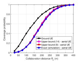
Figure 4: Coverage probability versus the collaboration distance $R_{c}$ for the aerial and ground UEs.

Fig. 4 shows the prominent effect of the collaboration distance $R_{c}$ on the coverage probability for two UEs, namely, ground UE, and high-altitude aerial UE. We can see that for both UEs, the coverage probability monotonically increases with $R_{c}$ since more SBSs cooperate to send a content when $R_{c}$ increases. Although the achievable coverage probability of the aerial UE is always upper bounded by that of the ground UE (due to the down-tilt of the SBSs’ antennas), we can see that the rate of improvement of the coverage probability with $R_{c}$, i.e., the slope, is higher for the aerial UE. This can be interpreted by the fact that increasing the collaboration distance yields more LoS signals within the desired signal side and mitigates them from the interference. In contrast, for the ground UE, the transmission is always dominated by NLoS signals and Rayleigh fading.

To show the effect of content availability, i.e., content caching, in Fig. 5, we plot the coverage probability versus the SIR threshold $\vartheta$ for different $c_{f}$. We observe that the coverage probability decreases as the caching probability $c_{f}$ decreases. This stems from the fact that the average number of caching SBSs decreases as $c_{f}$ decreases. This in turn reduces the cooperative transmission gain. Note that the value $c_{f}$ is, in fact, a parameter that can be designed based on various factors such as the memory size of SBSs, the popularity of files, and file library size.

V Conclusion

In this paper, we have proposed a novel framework for cooperative transmission and probabilistic caching suitable for high-altitude aerial UEs. In order to obtain analytically tractable expressions, we have employed Cauchy’s inequality and a second-order moment approximation of Gamma RVs to derive a closed-form upper bound on the content coverage probability. We have then shown that the derived bound is considerably tight. We have also shown that exploiting CoMP transmission with an average of 2.5 serving SBSs per cluster significantly improves the coverage probability, e.g., from $10\%$ to $70\%$ at $0\text{\,}\mathrm{d}\mathrm{B}$ SIR threshold. Moreover, comparing the performance of an aerial UE to a ground UE, our results have shown that the coverage probability of an aerial UE is always upper bounded by that of a ground UE owing to the down-tilted antenna pattern.

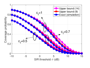
Figure 5: Coverage probability versus SIR threshold $\vartheta$ for different content caching probability $c_{f}$.

References

- [1] M. Vondra, M. Ozger, D. Schupke, and C. Cavdar, “Integration of satellite and aerial communications for heterogeneous flying vehicles,” IEEE Network, vol. 32, no. 5, pp. 62–69, September 2018.
- [2] U. Challita, W. Saad, and C. Bettstetter, “Deep reinforcement learning for interference-aware path planning of cellular-connected UAVs,” in Proc. of IEEE International Conference on Communications (ICC), Kansas City, USA, May 2018, pp. 1–7.
- [3] M. Mozaffari, W. Saad, M. Bennis, Y.-H. Nam, and M. Debbah, “A tutorial on UAVs for wireless networks: Applications, challenges, and open problems,” arXiv preprint arXiv:1803.00680, 2018.
- [4] M. Mozaffari, W. Saad, M. Bennis, and M. Debbah, “Unmanned aerial vehicle with underlaid device-to-device communications: Performance and tradeoffs,” IEEE Transactions on Wireless Communications, vol. 15, no. 6, pp. 3949–3963, June 2016.
- [5] Y. Zeng, J. Lyu, and R. Zhang, “Cellular-connected UAV: Potential, challenges and promising technologies,” IEEE Wireless Communications, October 2018.
- [6] Qualcomm, “LTE Unmanned aircraft systems’ trial report,” 2017.
- [7] M. M. Azari, F. Rosas, A. Chiumento, and S. Pollin, “Coexistence of terrestrial and aerial users in cellular networks,” in Proc. of IEEE Globecom Workshops (GC Wkshps), Singapore, Dec 2017, pp. 1–6.
- [8] M. M. Azari, F. Rosas, and S. Pollin, “Reshaping cellular networks for the sky: Major factors and feasibility,” in Proc. of IEEE International Conference on Communications (ICC), Kansas City, USA, May 2018, pp. 1–7.
- [9] X. Lin, V. Yajnanarayana, S. D. Muruganathan, S. Gao, H. Asplund, H.-L. Maattanen, M. Bergstrom, S. Euler, and Y.-P. E. Wang, “The sky is not the limit: LTE for unmanned aerial vehicles,” IEEE Communications Magazine, vol. 56, no. 4, pp. 204–210, April 2018.
- [10] B. Van der Bergh, A. Chiumento, and S. Pollin, “LTE in the sky: trading off propagation benefits with interference costs for aerial nodes,” IEEE Communications Magazine, vol. 54, no. 5, pp. 44–50, May 2016.
- [11] S. Zhang, Y. Zeng, and R. Zhang, “Cellular-enabled UAV communication: A connectivity-constrained trajectory optimization perspective,” arXiv preprint arXiv:1805.07182, 2018.
- [12] C. Zhu and W. Yu, “Stochastic modeling and analysis of user-centric network MIMO systems,” IEEE Transactions on Communications, pp. 1–1, 2018.
- [13] M. Haenggi, Stochastic geometry for wireless networks. Cambridge University Press, 2012.
- [14] M. Ding, P. Wang, D. López-Pérez, G. Mao, and Z. Lin, “Performance impact of LoS and NLoS transmissions in dense cellular networks,” IEEE Transactions on Wireless Communications, vol. 15, no. 3, pp. 2365–2380, March 2016.
- [15] P. Series, “Propagation data and prediction methods required for the design of terrestrial broadband radio access systems operating in a frequency range from 3 to 60 GHz,” 2013.
- [16] R. W. Heath Jr, T. Wu, Y. H. Kwon, and A. C. Soong, “Multiuser MIMO in distributed antenna systems with out-of-cell interference,” IEEE Transactions on Signal Processing, vol. 59, no. 10, pp. 4885–4899, Oct 2011.