An Analytical Approach to Improving Time Warping on Multidimensional Time Series

Abstract

Dynamic time warping (DTW) is one of the most used distance functions to compare time series, e. g. in nearest neighbor classifiers. Yet, fast state of the art algorithms only compare 1-dimensional time series efficiently. One of these state of the art algorithms uses a lower bound ($\texttt{LB}_{\texttt{Keogh}}$) introduced by E. Keogh to prune DTW computations. We introduce $\texttt{LB}_{\texttt{Box}}$ as a canonical extension to $\texttt{LB}_{\texttt{Keogh}}$ on multi-dimensional time series. We evaluate its performance conceptually and experimentally and show that an alternative to $\texttt{LB}_{\texttt{Box}}$ is necessary for multi-dimensional time series. We also propose a new algorithm for the dog-keeper distance (DK) which is an alternative distance function to DTW and show that it outperforms DTW with $\texttt{LB}_{\texttt{Box}}$ by more than one order of magnitude on multi-dimensional time series.

1 Introduction

Multimedia retrieval is a common application which requires finding similar objects to a query object. We consider examples such as gesture recognition with modern virtual reality motion controllers, GPS tracking, speech recognition, and classification of handwritten letters where the objects are multi-dimensional time series.

In many cases, similarity search is performed using a distance function on the time series, where small distances imply similar time series. A nearest neigbor query to the query time series can be a $k$-nearest neighbor ($k$-NN) query or an $\varepsilon$-nearest neighbor ($\varepsilon$-NN) query. A $k$-NN query retrieves the $k$ most similar time series. An $\varepsilon$-NN query retrieves all time series with a distance of at most $\varepsilon$.

A common application of $k$-NN queries is solving classification tasks in machine learning [9, 1]. For example, if all data objects (here time series) are labeled, a $k$-NN classifier basically assigns the label of a nearest neighbor to the unlabeled query object.

In our examples, the time series of the same classes, (e. g., same written character or same gestures) follow the same path in space, but have some temporal displacements. Tracking the GPS coordinates of two cars driving the same route from A to B is an illustrative example. We want these tracks (i. e. 2-dimensional time series) to be recognized as similar, although driving style, traffic lights, and traffic jams might result in temporal differences. Time warping distance functions such as dynamic time warping (DTW) [18], the dog-keeper distance (DK) [11], and the edit distance with real penalties (ERP) [8] respect this semantic requirement. They map pairs of time series representing the same trajectory to small distances.

We are interested in fast algorithms for $k$-NN queries based on these time series distance functions. Unfortunately, time warping distance functions usually have quadratic runtime [5, 6, 4].

However, we are usually not interested in the exact distance values but in the set of the nearest neighbors to our query time series. During such a nearest neighbor query, a common approach for improving the runtime is pruning as much distance computations as possible using lower bounds to the distance function: If the lower bound exceeds a certain threshold already (e. g. the largest distance to our $k$ nearest neighbors found so far), the expensive distance also yields a larger value and thus, its computation can be skipped.

E. Keogh proposed one of the state of the art algorithms for nearest neighbor queries with DTW on 1-dimensional time series. His main contribution is the lower bound $\texttt{LB}_{\texttt{Keogh}}$ [17, 14] pruning many expensive DTW computations during a linear scan.

1.1 Contributions

The contributions of this paper are the following:

• We introduce $\texttt{LB}_{\texttt{Box}}$ as canonical extension to $\texttt{LB}_{\texttt{Keogh}}$ for multi-dimensional time series in Section 3, i. e. $\texttt{LB}_{\texttt{Box}}$ is a lower bound to DTW on multi-dimensional time series and equals $\texttt{LB}_{\texttt{Keogh}}$ on 1-dimensional time series.

• In Section 3, we theoretically show, that the canonical extension $\texttt{LB}_{\texttt{Box}}$ suffers from an effect similar to the curse of dimensionality. In Section 5, we confirm the theoretical results with experiments on two synthesized and several real world data sets.

• In Section 4, we propose a new algorithm to compute the DK distance working faster than DTW with $\texttt{LB}_{\texttt{Box}}$ by more than one order of magnitude on multi-dimensional time series. The comparisons to DTW with $\texttt{LB}_{\texttt{Box}}$ in terms of accuracy and computation time are in Section 5.

We first declare basic notation and preliminaries in Section 1.2 and 2, respectively.

1.2 Basic Notation

We denote the natural numbers including zero with $\mathbb{N}$ and the real numbers with $\mathbb{R}$. Elements of a $d$-dimensional vector $v\in\mathbb{R}^{d}$ are accessed using subindices, i. e. $v_{3}$ is the third element of the vector. Sequences (here also called time series) are usually written using capital letters, e. g. $S=(s_{1},\cdots,s_{n})$ is a sequence of length $n$. Suppose $s_{i}\in\mathbb{R}^{d}$, then $s_{i,j}$ denotes the $j$-th element of the $i$-th vector in the sequence $S$. The projection to the $j$-th dimension is denoted via $S^{j}$, i. e. $S^{j}=(s_{1,j},\cdots,s_{n,j})$. The Euclidean norm of a vector $v$ is denoted via $\|v\|_{2}$, thus $\|v-w\|_{2}$ denotes the Euclidean distance between $v$ and $w\in\mathbb{R}^{d}$. In general, we denote distance functions via d.

We denote $[l,u]\subset\mathbb{R}$ as the 1-dimensional interval from $l\in\mathbb{R}$ to $u\in\mathbb{R}$. We denote the cartesian product using the symbol $\bigotimes$, thus $\bigotimes_{1\leqslant j\leqslant d}[l_{i},u_{i}]$ denotes the set of vectors $v$ with $l_{j}\leqslant v_{j}\leqslant u_{j}$ for $1\leqslant j\leqslant d$.

For a random variable $X$ over $\mathbb{R}$, we denote the mean with $\mathbb{E}[X]$, its variance using $\mathbb{V}[X]$, and the probability measure with $\mathbb{P}$, i. e. $\mathbb{P}[X<a]$ is the probability that the value of $X$ is less than $a\in\mathbb{R}$. We denote the standard normal distribution with $\Phi_{0,1}$.

2 Preliminaries

2.1 Time Warping Distance Functions

Dynamic time warping (DTW) is a distance function on time series [18]. Its benefit is a dynamic time alignment thus it is robust against time distortion or temporal displacements. Distance functions on time series which are robust against time distortion are from hereon called time warping distance functions.

For a formal definition, let $S=\left(s_{1},\cdots,s_{m}\right)$ and $T=\left(t_{1},\cdots,t_{n}\right)$ be two time series and d a distance function for the elements of the time series. DTW is defined recursively:

$$\texttt{DTW}{}(S,())= \ \infty\quad\texttt{DTW}{}((),T)=\infty$$

$$\texttt{DTW}{}((s),(t)) =\texttt{d}{}(s,t)^{2}$$

$$\texttt{DTW}{}(S,T)= \ d(s_{1},t_{1})^{2}+$$

$$\quad\quad\min\begin{cases}\texttt{DTW}{}(\texttt{Tail}(S),\texttt{Tail}(T))\\ \texttt{DTW}{}(S,\texttt{Tail}(T))\\ \texttt{DTW}{}(\texttt{Tail}(S),T)\end{cases}$$

where $\texttt{Tail}(T)\coloneqq\left(t_{2},\cdots,t_{n}\right)$. The dog-keeper distance (DK) is similar to DTW. It only differs by taking the maximum distance along a warping path instead of the sum.

$$\texttt{DK}{}(S,())=\ \infty\quad\texttt{DK}{}((),T)=\infty$$

$$\texttt{DK}{}((s),(t))=\texttt{d}{}(s,t)$$

$$\texttt{DK}{}(S,T)=$$

$$\quad\min\begin{cases}\max\left\{\texttt{d}{}(s_{1},t_{1}),\texttt{DK}{}(\texttt{Tail}(S),\texttt{Tail}(T))\right\}\\ \max\left\{\texttt{d}{}(s_{1},t_{1}),\texttt{DK}{}(S,\texttt{Tail}(T))\right\}\\ \max\left\{\texttt{d}{}(s_{1},t_{1}),\texttt{DK}{}(\texttt{Tail}(S),T)\right\}\end{cases}$$

Further examples for time warping distance functions are LCSS [19] and ERP [8].

Well known algorithms computing DTW and DK in quadratic time exist [18, 11]. These algorithms first build the cross product of both time series $S$ and $T$ using the distance function on the elements. The resulting distance matrix consists of entries $\texttt{d}{}(s_{i},t_{j})^{2}$ where $\texttt{d}{}(s_{1},t_{1})^{2}$ is in the bottom left cell and $\texttt{d}{}(s_{m},t_{n})^{2}$ is in the top right cell. After that, the algorithms compute the cheapest path from the bottom left to the top right cell by cell. For each cell, they replace the value with a combination of that value and the smallest value of one of the possible predecessors: the left, the lower, and the left lower neighbor cell, yielding the warping matrix. Unfortunately, any algorithm computing any of these distance functions has quadratic runtime complexity in worst case [6, 5].

2.2 Sakoe Chiba Band

The Sakoe Chiba band changes the semantic of DTW by constraining the possible paths in the warping matrix to a diagonal band of a certain bandwidth [18]. Thus, the warping of the time is constrained. On the other hand, the computation time is decreased since a huge part of the distance matrix does not need to be considered. Still, the runtime complexity remains quadratic because only a fixed ratio of the distance matrix is “cut off”.

2.3 Keoghs Lower Bound for DTW

Cheap lower bounds are used to prune many complete DTW computations and thus improve the overall computation time of a nearest neighbor search: If the lower bound already exceeds a desired threshold, then the final result of the expensive DTW distance function will be larger as well. Keogh proposed one of the most successfull lower bounding functions to DTW [14, 17]. His lower bound $\texttt{LB}_{\texttt{Keogh}}$ depends on the Sakoe Chiba Band which constrains finding best time alignments to a maximum time distance of a certain band width.

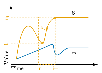
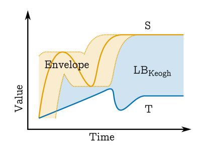
Figure 1: The envelope functions (computation sketched on the left) are used to compute the $\texttt{LB}_{\texttt{Keogh}}$ lower bound (right).

Basically, the idea of his lower bound is the following (cf. Figure 1 for an illustration): Consider two time series $S=\left(s_{1},\cdots,s_{m}\right)$ and $T=\left(t_{1},\cdots,t_{n}\right)$ and map each $s_{i}\in S$ to the interval of all possible aligned values within the time range (i. e. Sakoe Chiba band) $i-r$ and $i+r$:

$$l_{i} \coloneqq\min\left\{t_{i-r},\cdots,r_{i+r}\right\}$$

$$u_{i} \coloneqq\max\left\{t_{i-r},\cdots,r_{i+r}\right\}$$

Summing up the square distances of $s_{i}$ to each interval $[l_{i},u_{i}]$ is a lower bound to DTW since DTW aligns each $s_{i}$ to at least one of the values within $[l_{i},u_{i}]$, i. e.:

$$\texttt{LB}_{\texttt{Keogh}}{}(S,T) \coloneqq\sum_{i=1}^{m}\texttt{d}{}\left(s_{i},\left[l_{i},u_{i}\right]\right)^{2}\leqslant\texttt{DTW}{}(S,T)$$

where

$$\texttt{d}{}\left(s_{i},\left[l_{i},u_{i}\right]\right) \coloneqq\begin{cases}s_{i}-l_{i}&\text{iff }s_{i}<l_{i}\\ u_{i}-s_{i}&\text{iff }u_{i}<s_{i}\\ 0&\text{else}\end{cases}$$

The computation of the intervals $[l_{i},u_{i}]$ takes linear time when using the algorithm of Daniel Lemire [15]. Hence, it is obvious that the computation of $\texttt{LB}_{\texttt{Keogh}}$ is linear in the length of the time series as well.

3 Multi Dimensional Time Series

Consider two time series $S=\left(s_{1},\cdots,s_{m}\right)$ and $T=\left(t_{1},\cdots,t_{n}\right)$ with $s_{i},t_{j}\in\mathbb{R}^{k}$, i. e. $S$ and $T$ are multi-dimensional time series, and let

$$\texttt{d}{}(s_{i},t_{j}) \coloneqq\|s_{i}-t_{j}\|_{2}$$

be the Euclidean distance of the two vectors $s_{i}$ and $t_{j}$. We extend the lower bound $\texttt{LB}_{\texttt{Keogh}}$ of DTW canonically using the interpretation presented in Section 2.3: For each $s_{i}$ we find the minimal bounding box to all values $\left\{t_{i-r},\cdots,t_{i+r}\right\}$. Summing up the square distances of $s_{i}$ to their bounding boxes is again a lower bound to DTW.

For a formal definition, let

$$B_{i} \coloneqq\bigotimes_{1\leqslant j\leqslant k}\left[l_{i,j},u_{i,j}\right]$$

$$=\bigotimes_{1\leqslant j\leqslant k}\left[\min_{-r\leqslant\ell\leqslant r}t_{i+\ell,j},\max_{-r\leqslant\ell\leqslant r}t_{i+\ell,j}\right]$$

be the minimal axis aligned bounding box of $t_{i-r},\cdots,t_{i+r}$. The vectors $l_{i}$ and $u_{i}$ are the lower left and upper right corners, respectively. The distance of a vector to the bounding box is the distance to the nearest element within the bounding box:

$$\texttt{d}{}\left(s_{i},B_{i}\right)^{2} \coloneqq\min_{t\in B_{i}}\texttt{d}{}\left(s_{i},B_{i}\right)^{2}$$

$$=\min_{t\in B_{i}}\|s_{i}-t\|^{2}_{2}$$

$$=\sum_{1\leqslant j\leqslant k}\texttt{d}{}\left(s_{i},\left[l_{i,j},u_{i,j}\right]\right)^{2}$$

Considering the definition of DTW, the following function is a lower bound to DTW:

$$\texttt{DTW}{}(S,T) \geqslant$$

$$\texttt{LB}_{\Sigma\texttt{min}}{}(S,T) \coloneqq\sum_{i=1}^{m}\min_{-r\leqslant\ell\leqslant r}d\left(s_{i},t_{i+\ell}\right)^{2}$$

The distance function $\texttt{LB}_{\Sigma\texttt{min}}$ is hard to compute but can be estimated:

$$\texttt{LB}_{\Sigma\texttt{min}}{}(S,T)\geqslant\texttt{LB}_{\texttt{Box}}{}(S,T) \coloneqq\sum_{i=1}^{m}\texttt{d}{}\left(s_{i},B_{i}\right)^{2}$$

$$=\sum_{i=1}^{m}\sum_{j=1}^{k}\texttt{d}{}\left(s_{i},\left[l_{i,j},u_{i,j}\right]\right)^{2}$$

$$=\sum_{j=1}^{k}\texttt{LB}_{\texttt{Keogh}}{}\left(S^{j},T^{j}\right)$$ (1)

As it turns out, the estimation is not only a canonical extension of the lower bound proposed by Keogh, but it also can be computed by using his proposed algorithm on the different dimensions of the time series. Please note, that $\texttt{LB}_{\texttt{Box}}{}\equiv\texttt{LB}_{\texttt{Keogh}}{}$ holds especially for 1-dimensional time series.

Curse Of Dimensionality

Figure 2: Two 2-dimensional time series. DTW with Sakoe Chiba Band compares $q_{i}$ to at least one of $t_{i-r},\cdots,t_{i+r}$. $\texttt{LB}_{\texttt{Box}}$ compares $q_{i}$ to the corresponding bounding box $[l_{i,1},u_{i,1}]\otimes[l_{i,2},u_{i,2}]$.

Consider the bounding box of a subsequence $\left(t_{i-r},\cdots,t_{i+r}\right)$ as illustrated in Figure 2. For 2-dimensional time series, the following situation might happen: The time series $T$ moves along the left and then along the bottom edge of the bounding box. The query point $s_{i}$ however is at the top right vertex of the bounding box. Hence, a perfect alignment of DTW would still result in a distance

$$\texttt{LB}_{\Sigma\texttt{min}}{}(S,T) =\cdots+\min_{-r\leqslant\ell\leqslant r}\texttt{d}{}\left(s_{i},t_{i+\ell}\right)^{2}+\cdots>0$$

Simplifying the distance function to the bounding box results in

$$\texttt{LB}_{\texttt{Box}}{}(S,T) =\cdots+\sum_{j=1}^{k}\texttt{d}{}\left(s_{i},\left[l_{i,j},u_{i,j}\right]\right)^{2}+\cdots$$

$$=\cdots+0+\cdots=0$$

Thus, there is a clear divergence of DTW and $\texttt{LB}_{\texttt{Box}}$. With increasing dimensionality, there is more space for the time series to sneak past the query point, i. e. the probability for this situation to happen increases. For this reason, we claim that the tightness (i. e. the ratio $\frac{\texttt{LB}_{\texttt{Box}}{}}{\texttt{DTW}{}}$) of the lower bound gets worse with increasing dimensionality. This effect is similar to that of the Curse of Dimensionality [7], thus we still call it the same.

The goal of this section is the proof of Theorem 3.1 which claims the existence of the Curse of Dimensionality on $\texttt{LB}_{\texttt{Box}}$. Since we want to assume as little as possible from the data sets, we assume that the time series consist of independent and identical distributed elements. Section 5 confirms the theoretical results experimentally. For proving Theorem 3.1, we first need some technical lemmata.

Lemma 1.

Let $D_{\ell,j}$ be independent identically distributed random variables for $1\leqslant\ell\leqslant r$ and $1\leqslant j\leqslant k$. Furthermore, let $\mu_{r}\coloneqq\mathbb{E}\left[\min_{1\leqslant\ell\leqslant r}D_{\ell,j}\right]<\mu\coloneqq\mathbb{E}\left[D_{\ell,j}\right]$. Then,

$$\frac{\mathbb{E}\left[\sum_{j=1}^{k}\min_{1\leqslant\ell\leqslant r}D_{\ell,j}\right]}{\mathbb{E}\left[\min_{1\leqslant\ell\leqslant r}\sum_{j=1}^{k}D_{\ell,j}\right]}\rightarrow\frac{\mu_{r}}{\mu}<1\ \text{ for }k\rightarrow\infty.$$

Proof.

Let $\mu\coloneqq\mathbb{E}\left[D_{\ell,j}\right]$ be the mean and $\sigma^{2}\coloneqq\mathbb{V}\left[D_{\ell,j}\right]$ be the variance of the identically distributed variables $D_{\ell,j}$. The following inequation holds using calculation rules for expected values:

$$\mathbb{E}\left[\sum_{j=1}^{k}\min_{1\leqslant\ell\leqslant r}D_{\ell,j}\right] =k\cdot\mathbb{E}\left[\min_{1\leqslant\ell\leqslant r}D_{\ell,1}\right]=k\cdot\mu_{r}$$ (2)

Let $\rho\coloneqq\mathbb{E}\left[\left|D_{\ell,j}^{3}\right|\right]$. Since we only consider finite data sets for our nearest neighbour queries, $\rho<\infty$ holds obviously. For a theoretical analysis on data sets with infinite many elements, this property is a necessary preliminary in order to estimate the denominator using the Berry-Esseen Theorem. Basically, the Berry-Esseen Theorem claims that the sum of random variables converges to a normal distribution for increasing number of summands. We also apply the well known Markov inequality to estimate the denominator:

$$\mathbb{E}\left[\min_{1\leqslant\ell\leqslant r}\sum_{j=1}^{k}D_{\ell,j}\right]\geqslant a\cdot\mathbb{P}\left[\min_{1\leqslant\ell\leqslant r}\sum_{j=1}^{k}D_{\ell,j}\geqslant a\right]$$

$$=a\cdot\mathbb{P}\left[\bigvee_{1\leqslant\ell\leqslant r}\sum_{j=1}^{k}D_{\ell,j}\geqslant a\right]$$

$$=a\cdot\left(1-\mathbb{P}\left[\bigwedge_{1\leqslant\ell\leqslant r}\sum_{j=1}^{k}D_{\ell,j}<a\right]\right)$$

$$=a\cdot\left(1-\mathbb{P}\left[\sum_{j=1}^{k}D_{1,j}<a\right]^{r}\right)$$

$$=a\cdot\left(1-\mathbb{P}\left[\frac{\sum_{j=1}^{k}D_{1,j}-k\cdot\mu}{\sigma\sqrt{k}}<\frac{a-k\cdot\mu}{\sigma\sqrt{k}}\right]^{r}\right)$$

$$\geqslant a\cdot\left(1-\left(\Phi_{0,1}\left(\frac{a-k\cdot\mu}{k\sqrt{k}}\right)+\frac{C\cdot\rho}{\sigma^{3}\cdot\sqrt{k}}\right)^{r}\right)$$

$$=k\cdot\mu\cdot\left(1-\left(\frac{C\cdot\rho}{\sigma^{3}\cdot\sqrt{k}}\right)^{r}\right)\text{ for }a=k\cdot\mu$$ (3)

where the first inequation is the Markov inequality and the second inequation is derived from the Berry-Esseen Theorem which also claims the existence of the constant $C$.

Putting together Equation (2) and Inequation (3), we achieve the desired convergence:

$$\frac{\mathbb{E}\left[\sum_{j=1}^{k}\min_{1\leqslant\ell\leqslant r}D_{\ell,j}\right]}{\mathbb{E}\left[\min_{1\leqslant\ell\leqslant r}\sum_{j=1}^{k}D_{\ell,j}\right]} \leqslant\frac{k\cdot\mu_{r}}{k\cdot\mu\cdot\left(1-\left(\frac{C\cdot\rho}{\sigma^{3}\cdot\sqrt{k}}\right)^{r}\right)}$$

$$\longrightarrow\frac{\mu_{r}}{\mu}\text{ for }k\rightarrow\infty$$

$\square$

For $r=R\cdot n$ ($0<R\leqslant 1$), the following Lemma 2 shows that the value $\frac{\mu_{r}}{\mu}$ from Lemma 1 converges to $0$ for $n\rightarrow\infty$.

Lemma 2.

Let $X_{i}\geqslant 0$ be independent identically distributed random variables for $1\leqslant i\leqslant n$ such that $\mathbb{P}\left[X_{i}\geqslant x\right]<1$ for each $x>0$. Then, $\mathbb{E}\left[\min_{1\leqslant i\leqslant n}X_{i}\right]\longrightarrow 0$ for $n\rightarrow\infty$.

Proof.

The expected value can be calculated as follows:

$$\mathbb{E}\left[\min_{1\leqslant i\leqslant n}X_{i}\right] =\int_{0}^{\infty}\mathbb{P}\left[\min_{1\leqslant i\leqslant n}X_{i}\geqslant x\right]dx$$

$$=\int_{0}^{\infty}\mathbb{P}\left[X_{1}\geqslant x\wedge\cdots\wedge X_{n}\geqslant x\right]dx$$

$$=\int_{0}^{\infty}\mathbb{P}\left[X_{i}\geqslant x\right]^{n}dx$$

Since $\mathbb{P}\left[X_{i}\geqslant x\right]$ is Lebesgue measurable and $\mathbb{P}\left[X_{i}\geqslant x\right]^{n}\longrightarrow 0$ for $x>0$, the last integral converges to zero for $n\rightarrow\infty$. $\square$

Now, we prove that $\texttt{LB}_{\texttt{Box}}$ suffers from the curse of dimensionality using Lemma 1 and 2, i. e. the tightness of the lower bound $\texttt{LB}_{\texttt{Box}}$ to DTW gets worse for increasing dimensionality.

Theorem 3.1.

Let $S$ and $T$ be two time series in $\mathbb{R}^{k}$ with length $n$. Then

$$\frac{\mathbb{E}\left[\texttt{LB}_{\texttt{Box}}{}(S,T)\right]}{\mathbb{E}\left[\texttt{DTW}{}(S,T)\right]}\longrightarrow 0$$

for $k,n\rightarrow\infty$.

Proof.

Since we do not know anything about the time series, we assume that their elements are independent identically distributed variables. For simplicity, we even assume that the distance between any two elements is a random variable, i. e.

$$D_{i,j} \coloneqq\texttt{d}{}\left(s_{i},t_{j}\right)^{2}$$

are independent identically distributed random variables. With a Sakoe Chiba band of width $r=R\cdot n$ ($0<R\leqslant 1$ constant) we get

$$\frac{\mathbb{E}\left[\texttt{LB}_{\texttt{Box}}{}(S,T)\right]}{\mathbb{E}\left[\texttt{DTW}{}(S,T)\right]} \leqslant\frac{\mathbb{E}\left[\sum_{i=1}^{n}\sum_{j=1}^{k}\texttt{d}{}\left(s_{i},\left[l_{i,j},r_{i,j}\right]\right)^{2}\right]}{\mathbb{E}\left[\texttt{LB}_{\Sigma\texttt{min}}{}(S,T)\right]}$$

$$\leqslant\frac{\mathbb{E}\left[\sum_{i=1}^{n}\sum_{j=1}^{k}\min_{-r\leqslant\ell\leqslant r}D_{i+\ell,j}\right]}{\mathbb{E}\left[\sum_{i=1}^{n}\min_{-r\leqslant\ell\leqslant r}\sum_{j=1}^{k}D_{i+\ell,j}\right]}$$

$$=\frac{n\cdot\mathbb{E}\left[\sum_{j=1}^{k}\min_{1\leqslant\ell\leqslant 2r+1}D_{\ell,j}\right]}{n\cdot\mathbb{E}\left[\min_{1\leqslant\ell\leqslant 2r+1}\sum_{j=1}^{k}D_{\ell,j}\right]}$$

$$\longrightarrow\frac{\mu_{r}}{\mu}\quad\text{ for }k\rightarrow\infty$$

$$\longrightarrow 0\quad\text{ for }n\rightarrow\infty$$

$\square$

4 Dog-Keeper Distance

Practical implementations of DTW speed up the computation process by stopping early when a promised lower bound already exceeds a certain threshold. For example, processing the warping matrix while computing DTW, the minimum value of a column or row is a lower bound to the final distance value. The lower bound proposed by Keogh promises even tighter values to the final distance value [17].

Since DTW sums up values along a warping path through the distance matrix, the values in the early computation time exceed a certain threshold less probable than the values at a later computation time. This observation does not hold when computing the DK distance [2]. This insight yields the idea that the matrix filled out during computation of the DK distance might be very sparse.

Therefore, our approach to improving the computation time of the DK distance is to compute the distance matrix using a sparse matrix algorithm (cf. Section 4.2). However, to avoid computing most of the cells of this matrix, we need a low threshold beforehand. Such a threshold is found using a cheap upper bound to the DK distance. Specifically, we propose a greedy algorithm to the time warping alignment problem (cf. 4.1).

To explain the algorithms in detail, consider two time series $S=(s_{1},\cdots,s_{m})$ and $T=(t_{1},\cdots,t_{n})$.

4.1 Greedy Dog-Keeper

The greedy dog-keeper distance (GDK) starts by aligning $s_{1}$ and $t_{1}$. It then successively steps to one of the next pairs aligning $(s_{i+1},t_{j})$, $(s_{i},t_{j+1})$, or $(s_{i+1},t_{j+1})$ with the lowest distance. When it reaches the alignment of $s_{m}$ to $t_{n}$, the maximum of the distances along the choosen path yields the final distance. Algorithm 1 provides the pseudo code for the algorithm.

Algorithm 1 Greedy dog-keeper distance

⬇

1Algorithm: greedydogkeeper

2Input: time series $S,T$ of length $m,n$ resp.; threshold $\varepsilon$

3Output: upper bound $d$

4

5let $(i,j)=(1,1)$

6let $g=\texttt{d}{}\left(s_{i},t_{j}\right)$

7while $i\neq m$ and $j\neq n$

8 // non defined distances yield $\infty$

9 $(i,j)=\arg\min\begin{cases}\texttt{d}{}(s_{i+1},t_{j})\\ \texttt{d}{}(s_{i+1},t_{j+1})\\ \texttt{d}{}(s_{i},t_{j+1})\end{cases}$

10 $g=\max\left\{g,\texttt{d}{}(i,j)\right\}$

11 if $g>\varepsilon$ then return $g$

12return $g$

So far, the GDK distance matches whole sequences against each other. In order to support sub sequence matching, we alter the algorithm by first finding the best match of $s_{1}$ to any $t_{i}$ (name it $t_{left}$). Then, we run GDK starting at $t_{left}$ and stop the computation as soon, as $s_{m}$ is aligned to one of the $t_{i}$. For details, refer to Algorithm 2.

Algorithm 2 Greedy dog-keeper for Sub Sequence Search

⬇

1Algorithm: greedydogkeeper

2Input: time series $S$ and $T$ of length $m$ and $n$ resp., threshold $\varepsilon$

3Output: upper bound $d$

4

5let $(i,j)=(1,\arg\min\left\{\texttt{d}{}(s_{1},t_{j})\right\})$

6let $g=\texttt{d}{}\left(s_{i},t_{j}\right)$

7while $i\neq m$

8 // non defined distances yield $\infty$

9 $(i,j)=\arg\min\begin{cases}\texttt{d}{}(s_{i+1},t_{j})\\ \texttt{d}{}(s_{i+1},t_{j+1})\\ \texttt{d}{}(s_{i},t_{j+1})\end{cases}$

10 $g=\max\left\{g,\texttt{d}{}(i,j)\right\}$

11 if $g>\varepsilon$ then return $g$

12return $g$

Both algorithms have linear complexity, since the while loop runs at maximum $m+n$ times

4.2 Sparse dog-keeper distance

The sparse dog-keeper algorithm essentially works the same as the original algorithm, except that it only visits those neighbor cells of the distance matrix having a value not larger than a given threshold. Algorithm 3 provides the pseudo code for the algorithm: Similar to the original algorithm, we compute the (sparse) warping matrix column by column (cf. Line 10). The variables $I$ and $J$ store the indices of cells to visit in the current and next column, respectively. If the value at the current cell of the matrix is not larger than the threshold (cf. Line 13), we also need to visit the right, upper right, and upper cells (cf. Lines 15 and 16). The actual values within the columns are stored in $D$ (current column) and $E$ (previous column). After we finished the computation of a column, we prepare the variables to enter the next column (cf. Lines 19 to 26).

Algorithm 3 Sparse dog-keeper distance

⬇

1Algorithm: sparsedogkeeper

2Input: time series $S$ and $T$ of length $m$ and $n$ resp., threshold $\varepsilon$, boolean SUB

3Output: distance $d$

4

5$I=\left\{1\right\}$

6$J=\emptyset$

7$D=(\infty,\cdots)$

8$E=(\infty,\cdots)$

9

10for $k=1$ to $n$

11 if SUB $d=\infty$

12 for $i\in I$

13 if $\texttt{d}{}\left(S_{i},T_{k}\right)\leqslant\varepsilon$

14 $D_{i}=\max\begin{cases}\texttt{d}{}\left(S_{i},T_{k}\right)\\ \min\left\{D_{i-1},E_{i},E_{i-1}\right\}\end{cases}$

15 $I=I\cup\left\{i+1\right\}$

16 $J=J\cup\left\{i,i+1\right\}$

17 else

18 $I=I\setminus\left\{i\right\}$

19 if SUB $d=\min\left\{d,D_{m}\right\}$

20 $E=D$

21 // reset $D$ to $(\infty,\cdots)$

22 for $i\in I$

23 $D_{i}=\infty$

24 if SUB $I=J\cup\left\{1\right\}$

25 else $I=J$

26 $J=\emptyset$

27 if not SUB and $I$ is empty

28 return $\varepsilon$

29

30if SUB return $d$

31else return $D_{m}$

The algorithm performs subsequence search iff passing true for the parameter SUB. It differs to the whole matching version by considering each position of the super sequence as possible start of a match (cf. Line 24) and by considering each position as possible end of a match (cf. Line 19).

4.3 Nearest Neighbour Search

Our nearest neighbor search algorithm requires finding a good upper bound. Hence, we first loop over all time series and find the lowest upper bound using the GDK distance. Then, we perform a common nearest neighbor search by scanning the time series.

5 Evaluation

In Section 5.1, we evaluate Theorem 3.1 (which claims the existence of the curse of dimensionality for $\texttt{LB}_{\texttt{Box}}$) experimentally on synthetic data sets which have a parameter for setting the dimensionality [3]. We confirm our observations on real world data sets.

We compare DTW (with $\texttt{LB}_{\texttt{Box}}$ as lower bound) against our implementation of the DK distance in terms of runtime in Section 5.2. We focus on the subsequence matching algorithms since this is the more challenging task.

The retrieval quality is of high importance when considering an alternative distance function for nearest neighbor queries. Therefore, we close the evaluation by comparing the accuracy of the DK and DTW distance functions on nearest neighbor tasks in Section 5.3.

Synthetic Data Sets

Due to space limitations, we can not show results for all parameters of the data set generators. The following set of parameters yield the most interesting results: If not mentioned otherwise explicitely, we generate data with distortion $25$, radius $50$, $50$ distinguish classes, and $2$ representatives per class using the RAM generator and $27$ distinguish classes and $3$ representatives per class using the CBF generator.

5.1 Curse Of Dimensionality

Theorem 3.1 claims that the tightness of the lower bound function $\texttt{LB}_{\texttt{Box}}{}$ to DTW gets worse with increasing dimensionality. We evaluate the theorem experimentally on data sets generated by the two synthesizers CBF and RAM [3]. Figure 3 illustrates examples for time series generated by the RAM and CBF synthesizers.

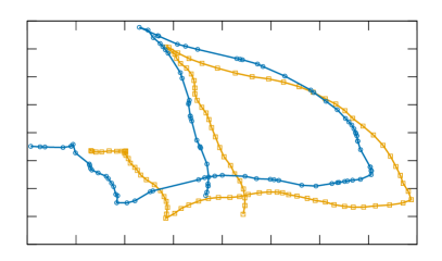
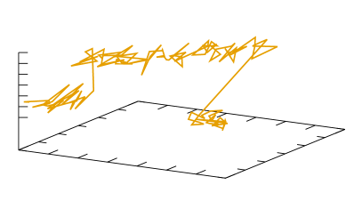
Figure 3: Two 2-dimensional examples for the RAM data set (left) and one example for the CBF data set (right).

Implementation

Our implementation of $\texttt{LB}_{\texttt{Box}}$ is based on $\texttt{LB}_{\texttt{Keogh}}$ from the UCR Suite [17]. We skipped the normalization on some data sets to improve the runtime and accuracy of $\texttt{LB}_{\texttt{Box}}$. While adapting the UCR Suite to work on multi-dimensional time series, we checked that the runtime remained stable for 1-dimensional time series. Thus, we made sure that all of our results for runtime comparison are not implementation dependent. We ran all experiments on one core of an Intel(R) Xeon(R) CPU E5-2620 0 @ 2.00GHz with 24GB Memory.

Tightness

Figure 5 demonstrates that the tightness of $\texttt{LB}_{\texttt{Box}}$ to DTW is decreasing down to zero for increasing length, which confirms Theorem 3.1. The theorem also claims that the tightness drops to a constant value for increasing dimensionality but constant length. With Figure 5 we confirm this claim for the RAM data sets and show even more that the tightness converges (drops down) already for moderate dimensionality (e. g. 3 dimensional time series). We could ovbserve the same results for the CBF data sets (cf. Figure 6) although the dimensionality has greater impact on the tightness while the length has a smaller impact.

Pruning power

We show the effects on the pruning power in the second heat maps of both Figures 5 and 6. Their black lines (lines of same values within each heat map) look rather similar to the black lines in their corresponding heat maps on the left side. They confirm the correlation between the dropping of the tightness of $\texttt{LB}_{\texttt{Box}}$ and the dropping of the pruning power within a nearest neighbor search. Still, the dimensionality has a larger impact to the pruning power than to the tightness of the time series.

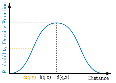
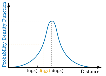
Figure 4: Two data sets (left: low dimensional; right: high dimensional), a query $q$, a nearest neighbor $y$ and a candidate $x$. If the lower bound $l(q,x)\geqslant d(q,y)$, then $x$ can be pruned without computation of $d(q,x)$.

The reason is the curse of dimensionality on retrieval tasks [7]. It basically says that the variance of distance values between random elements of a data set decreases with increasing dimensionality. Thus, even if the tightness of a lower bound such as $\texttt{LB}_{\texttt{Box}}$ equals on two distinct data sets, pruning is less probable in the higher dimensional data set. Figure 4 illustrates an example where $q$ is the query and $y$ the nearest neighbor found so far during the search. If the lower bound $l(q,x)$ is larger than $d(q,y)$ then we can prune the next element $x$. Assume $l(q,x)=\alpha\cdot d(q,x)$ where $0\leqslant\alpha\leqslant 1$ is equal in the low dimensional and the high dimensional data set. Since $d(q,x)$ and $d(q,y)$ converge on data sets with increasing dimensionality (this is the curse of dimensionality), $l(q,x)<d(q,y)\approx d(q,x)$ is more probable in higher dimensionality. The lower bound can not be used for pruning in these cases. Please note, that this insight holds for any lower bound driven approach.

Both of the Figures 5 and 6 show that $\texttt{LB}_{\texttt{Box}}$ loses its benefit already for moderate dimensionality.

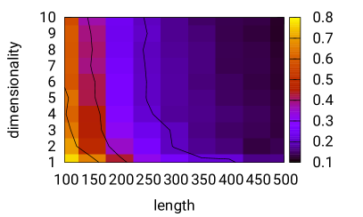
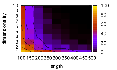
Figure 5: Heat maps presenting the average tightness of $\texttt{LB}_{\texttt{Box}}$ (left) and the pruning power of $\texttt{LB}_{\texttt{Box}}$ in percent (right) on the RAM data set.

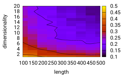
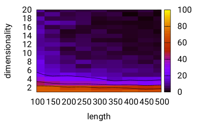
Figure 6: Heat maps presenting the average tightness of $\texttt{LB}_{\texttt{Box}}$ (left) and the pruning power of $\texttt{LB}_{\texttt{Box}}$ in percent (right) on the CBF data set.

5.2 Computation Time

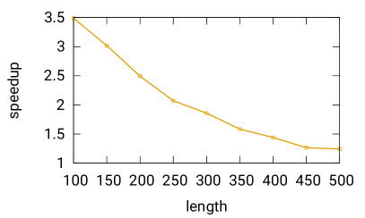
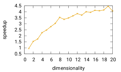
Figure 7: Speedup of DK to DTW with $\texttt{LB}_{\texttt{Box}}$ on the CBF data set. Dimensionality: 10 (left); Length: 100 (right).

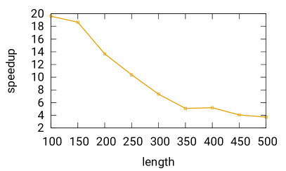
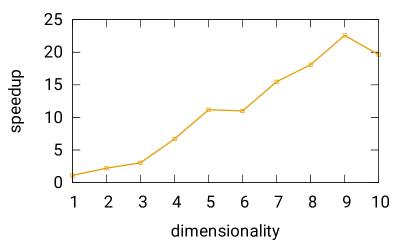
Figure 8: Speedup of DK to DTW with $\texttt{LB}_{\texttt{Box}}$ on the RAM data set. Dimensionality: 10 (left); Length: 100 (right).

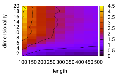
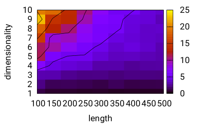
Figure 9: Speedup of DK to DTW with $\texttt{LB}_{\texttt{Box}}$ on the CBF data set (left) and the RAM data set (right). Dimensionality: 10 (left); Length: 100 (right).

For the evaluation of the runtime of our DK algorithm, we consider the runtime of DTW with $\texttt{LB}_{\texttt{Box}}$ as the base line. In Figures 7 and 8 we show the speedup of our DK implementation against DTW with $\texttt{LB}_{\texttt{Box}}$ on the RAM and CBF data sets, respectively. The speedup decreases for longer time series while increasing with growing dimensionality. Figure 9 confirms this observation on an even larger parameter set. Thus, our DK implementation outperforms DTW with $\texttt{LB}_{\texttt{Box}}$ on rather short and multi-dimensional time series.

To ensure that our results do not depend on the generated synthetical data sets, we repeated the same experiments on the following real world data sets from the UCI Machine Learning Repository [10]: Character Trajectories (CT), Activity Recognition system based on Multisensor data fusion (AReM) [16], EMG Physical Action (EMGPA), Australian Sign Language 2 (ASL) [13], Arabic Spoken Digits (ASD), and Vicon Physical Action (VICON). We also used the ECG data proposed by Keogh [17] for querying in one very long time series. Columns 1 and 2 of Table 1 show that the speedup increases with growing dimensionality. Thus, we demonstrate that our implementation of the DK distance outperforms DTW with $\texttt{LB}_{\texttt{Box}}$ in terms of computation time, especially on multi-dimensional time series.

Table 1: Speedup and Accuracy of DTW with $\texttt{LB}_{\texttt{Box}}$ and DK on real world data sets.

data set	dim.	speedup	acc. DTW	acc. DK
ECG	1	$0.05$	-	-
CT	2	$4.5$	$0.94$	$0.93$
AReM	6	$1.2$	$0.81$	$0.75$
EMGPA	8	$31$	$0.21$	$0.26$
ASD	13	$45$	$0.98$	$0.96$
ASL	22	$33$	$0.85$	$0.88$
VICON	27	$62$	$0.12$	$0.09$

5.3 Retrieval Quality:

Figures 10 and 11 reveal that the accuracy of both distance functions decreases on CBF while increasing on RAM with growing dimensionality. While DK outperforms DTW on the CBF data set it looses on the RAM data set.

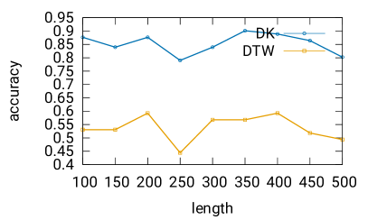
Figure 10: Accuracy of DK and DTW with $\texttt{LB}_{\texttt{Box}}$ on the CBF data set. Dimensionality: 10 (left); Length: 100 (right).

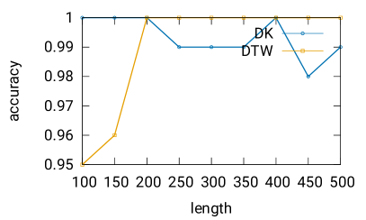
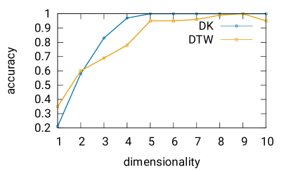
Figure 11: Accuracy of DK and DTW with $\texttt{LB}_{\texttt{Box}}$ on the RAM data set. Dimensionality: 10 (left); Length: 100 (right).

Columns 1, 3 and 4 of Table 1 also prove that there is no clear winner regarding accuracy.

6 Conclusion

We introduced $\texttt{LB}_{\texttt{Box}}$ as a canonical extension to Keogh’s lower bound $\texttt{LB}_{\texttt{Keogh}}$ for DTW on multi-dimensional time series and proved its correctness. Not only do lower bounds suffer from the curse of dimensionality even if their tightness remains constant, but we also proved that the tightness of $\texttt{LB}_{\texttt{Box}}$ decreases with growing dimensionality. On the other hand, we proposed an alternative algorithm for the computation of the long known DK distance, which is similar to DTW. Please note that the DK distance satisfies the triangle inequality and can thus be used in metric indexes [12, 2].

In our evaluation, we confirmed our theory that $\texttt{LB}_{\texttt{Box}}$ as extension of $\texttt{LB}_{\texttt{Keogh}}$ suffers from the curse of dimensionality. We could show that our implementation of DK outperforms $\texttt{LB}_{\texttt{Box}}$ on multi-dimensional synthesized data sets as well as real world data sets in terms of computation time by more than one order of magnitude. However, there is no clear winner regarding the accuracy in retrieval tasks. Hence, we propose to stay with $\texttt{LB}_{\texttt{Keogh}}$ on 1-dimensional time series while choosing the DK distance on multi-dimensional time series.

7 Acknowledgments

We like to thank Jochen Taeschner for his help on this work.

References

- [1] Miscellaneous Clustering Methods, pages 215–255. Wiley-Blackwell, 2011.
- [2] J. P. Bachmann and J.-C. Freytag. Dynamic Time Warping and the (Windowed) Dog-Keeper Distance, pages 127–140. Springer International Publishing, Cham, 2017.
- [3] J. P. Bachmann and J.-C. Freytag. High Dimensional Time Series Generators, 2018. arXiv:1804.06352v1.
- [4] A. Backurs and P. Indyk. Edit distance cannot be computed in strongly subquadratic time (unless SETH is false). CoRR, abs/1412.0348, 2014.
- [5] K. Bringmann. Why walking the dog takes time: Frechet distance has no strongly subquadratic algorithms unless SETH fails. CoRR, abs/1404.1448, 2014.
- [6] K. Bringmann and M. Künnemann. Quadratic conditional lower bounds for string problems and dynamic time warping. CoRR, abs/1502.01063, 2015.
- [7] E. Chávez, G. Navarro, R. Baeza-Yates, and J. L. Marroquín. Searching in metric spaces. ACM Comput. Surv., 33(3):273–321, Sept. 2001.
- [8] L. Chen and R. Ng. On the marriage of lp-norms and edit distance. In Proceedings of the Thirtieth International Conference on Very Large Data Bases - Volume 30, VLDB ’04, pages 792–803. VLDB Endowment, 2004.
- [9] D. Coomans and D. Massart. Alternative k-nearest neighbour rules in supervised pattern recognition: Part 1. k-nearest neighbour classification by using alternative voting rules. Analytica Chimica Acta, 136:15 – 27, 1982.
- [10] D. Dheeru and E. Karra Taniskidou. UCI machine learning repository, 2017.
- [11] T. Eiter and H. Mannila. Computing discrete fréchet distance. Technical report, Technische Universität Wien, 1994.
- [12] M. R. Fréchet. Sur quelques points du calcul fonctionnel. 22. Rendiconti del Circolo Mathematico di Palermo, 1906.
- [13] M. W. Kadous. Temporal Classification: Extending the Classification Paradigm to Multivariate Time Series. PhD thesis, New South Wales, Australia, Australia, 2002. AAI0806481.
- [14] E. Keogh and C. A. Ratanamahatana. Exact indexing of dynamic time warping. Knowledge and Information Systems, 7(3):358–386, 2005.
- [15] D. Lemire. Faster retrieval with a two-pass dynamic-time-warping lower bound. Pattern Recogn., 42(9):2169–2180, Sept. 2009.
- [16] F. Palumbo, C. Gallicchio, R. Pucci, and A. Micheli. Human activity recognition using multisensor data fusion based on reservoir computing. 8:87–, 03 2016.
- [17] T. Rakthanmanon, B. Campana, A. Mueen, G. Batista, B. Westover, Q. Zhu, J. Zakaria, and E. Keogh. Searching and mining trillions of time series subsequences under dynamic time warping. In Proceedings of the 18th ACM SIGKDD International Conference on Knowledge Discovery and Data Mining, KDD ’12, pages 262–270, New York, NY, USA, 2012. ACM.
- [18] H. Sakoe and S. Chiba. Readings in speech recognition. In A. Waibel and K.-F. Lee, editors, Readings in Speech Recognition, chapter Dynamic Programming Algorithm Optimization for Spoken Word Recognition, pages 159–165. Morgan Kaufmann Publishers Inc., San Francisco, CA, USA, 1990.
- [19] M. Vlachos, M. Hadjieleftheriou, D. Gunopulos, and E. Keogh. Indexing multi-dimensional time-series with support for multiple distance measures. In Proceedings of the Ninth ACM SIGKDD International Conference on Knowledge Discovery and Data Mining, KDD ’03, pages 216–225, New York, NY, USA, 2003. ACM.