Advanced control laws for the new generation of AO systems

Abstract

Geared by the increasing need for enhanced performance, both optical and computational, new dynamic control laws have been researched in recent years for next generation adaptive optics systems on current 10 m-class and extremely large telescopes up to 40 m. We provide an overview of these developments and point out prospects to making such controllers drive actual systems on-sky.

1 Introduction

Adaptive optics systems rely on some form of dynamic control to keep up with the evolving atmospheric and telescope disturbances [1, 2]. Although historically in closed-loop, open-loop systems have also been deployed on-sky [3, 4]. The developments covered here apply to both configurations.

The need for faster systems with increased performance led to the development of minimum-variance (MV) controllers that can potentially cope with the very large number of degrees of freedom (DoF) in the order of many thousands [5, 6, 7]. The main shortcoming is the computational burden associated and how these solutions can be mapped onto real-time architectures to drive systems at kilohertz frame-rates.

In this contribution we provide an overview of recent work on optimal and near-optimal solutions for both classical and tomographic systems. We cover ways in which disturbance’s temporal evolution can be embedded in the control to improve contrast in extreme AO systems by tackling servo-lag errors causing poorer performance at short separations from the host star. For tomographic systems we reason analogously to provide insight into how spatio-temporal combinations can lead to improved performance.

The use of sub-optimal, ad-hoc controllers in AO is commonplace [1, 2]. Historically, integral-action controllers were (and are still) the most common choice for a variety of good reasons

• AO being a disturbance-rejection dynamical problem [8], driving the measurement error (i.e. the sum of disturbance and propagated noise – see Fig. 1) to zero is a sound approach

• ease of manipulation with reduced number of free-parameters [9, 10, 11] – basically the controller gain

• synthetic modelling in open- and closed-loop [12, 13, 14, 15] for which closed-forms exist

It it worth pointing out that such integral-action control is the first choice to drive the single-conjugate (SCAO) and high-order laser-guide-star assisted tomographic systems on all the three giant telescopes [16, 17, 18].

For low-order modes however there is a general consensus on the need for more advanced controllers capable of improved performance [19, 20, 21]. A brief presentation is provided next.

2 Towards Strehl-optimal control

Turning our attention now to Strehl-ratio optimisation (a metric of image quality between 1 for aberration-free diffraction-limited images converging asymptotically to 0 for totally uncorrected images), it has been shown in Herrman et al (1992) [22] that minimising the residual phase error variance (MV) is a surrogate for maximising the Strehl-ratio. This makes for a discrete-time minimum residual phase variance (MV) criterion.

To address this class of optimisation problems, we start off by a general discrete-time linear-quadratic (LQ) regulator minimizes the cost function

$$J({\mathbf{u}})=\lim_{M\rightarrow\infty}\frac{1}{M}\sum_{k=0}^{M-1}\left({\mathbf{x}}^{\mathsf{T}}\mathbf{Q}{\mathbf{x}}+{\mathbf{u}}^{\mathsf{T}}\mathbf{R}{\mathbf{u}}+2{\mathbf{x}}^{\mathsf{T}}\mathbf{S}{\mathbf{u}}\right)_{k}$$ (1)

where the weighting triplet $\{\mathbf{Q},\mathbf{R},\mathbf{S}\}$ is made apparent and will be specified next by developing an AO-specific quadratic criterion subject to the state-space model

$$\left\{\begin{array}[]{ccl}{\mathbf{x}}_{k+1}&=&\mathcal{A}_{\mathsf{tur}}{\mathbf{x}}_{k}+\mathcal{V}\mathbf{\nu}_{k}\\ {\mathbf{s}}_{{\mathbf{\alpha}},k}&=&\mathcal{C}_{\mathsf{tur}}{\mathbf{x}}_{k}+\mathcal{D}_{\mathsf{tur}}{\mathbf{u}}_{k-d}+{\mathbf{\eta}}_{k}\end{array}\right.$$ (2)

where ${\mathbf{x}}_{k}$ is the state vector that contains if not the phase directly a linear combination thereof, ${\mathbf{s}}_{{\mathbf{\alpha}},k}$ are the noisy measurements provided by the WFS in the GS directions ${\mathbf{\alpha}}$, $\mathbf{\nu}_{k}$ and ${\mathbf{\eta}}_{k}$ are spectrally white, Gaussian-distributed state excitation and measurement noise respectively. In the following we assume that the state drive noise covariance $\mathbf{\Sigma}_{\mathbf{\nu}}=\left\langle{\mathbf{\nu}\mathbf{\nu}^{\mathsf{T}}}\right\rangle$ and measurement noise covariance $\mathbf{\Sigma}_{\mathbf{\mathbf{\eta}}}=\left\langle{\mathbf{\eta}\mathbf{\eta}^{\mathsf{T}}}\right\rangle$ are known and that $\mathbf{\Sigma}_{\mathbf{\mathbf{\eta,\nu}}}=\left\langle{\mathbf{\eta}\mathbf{\nu}^{\mathsf{T}}}\right\rangle=0$. Matrices $\mathcal{A}_{\mathsf{tur}},\mathcal{B}_{\mathsf{tur}},\mathcal{C}_{\mathsf{tur}}$ will be populated according to the temporal evolution and measurement modes of the AO loop.

The solution to the criterion in Eq. (2) is known to be a negative state feedback of the form [8]

$${\mathbf{u}}_{k}=-\mathbf{K}_{\infty}{\mathbf{x}}_{k}$$ (3)

where $\mathbf{K}_{\infty}$ is the LQ gain which involves the solution of a Riccati equation [8]. The AO problem allows for a simplification leading to an easier to grasp solution.

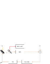
Figure 1: (Colour on-line) Control-oriented block diagram in closed-loop. The residual error ${\mathbf{\varepsilon}}$ is a joint contribution od the phase ${\mathbf{\psi}}$ and noise ${\mathbf{\eta}}$. In this paper we focus on the choice of the controller, assuming the rest of the loop to be represented by pure delays.

Looking back at the AO optimisation criterion, it takes the form

$$J({\mathbf{u}})=\lim_{M\rightarrow\infty}\frac{1}{M}\sum_{k=0}^{M-1}\sigma^{2}_{k}\\ =\lim_{M\rightarrow\infty}\frac{1}{M}\sum_{k=0}^{M-1}\|{\mathbf{\psi}}_{k+1}(\mathbf{\rho},{\mathbf{\beta}})-\mathbf{N}{\mathbf{u}}_{k}(\mathbf{\rho},{\mathbf{\beta}})\|^{2}_{W,L_{2}(\Omega)}$$

where ${\mathbf{\psi}}_{k+1}$ is the average phase disturbance $\in[kT_{s}:(k+1)T_{s}[$, ${\mathbf{u}}_{k}$ is the applied commands over $\in[kT_{s}:(k+1)T_{s}[$ producing a correction phase $\mathbf{N}{\mathbf{u}}_{k}(\mathbf{\rho},{\mathbf{\beta}})$ with $\mathbf{N}$ a concatenation of deformable-mirror (DM) influence functions and $\mathbf{\rho}$ a bi-dimensional spatial index spanning the telescope pupil and ${\mathbf{\beta}}$ the observation direction of interest. In Eq. (2), $W$ is a positive-definite weighting matrix that removes the piston contribution over the telescope aperture and $L_{2}$ the Euclidean norm over the aperture $\Omega$ such that $\sigma^{2}_{k}=\|{\mathbf{\varepsilon}}_{k}\|^{2}_{W,L_{2}(\Omega)}={\mathbf{\varepsilon}}_{k}^{\mathsf{T}}W{\mathbf{\varepsilon}}_{k}$. Equation (2) neglects any WF dynamics during the integration. The error that is neglected here has been dubbed insurmountable error due to the use of averaged variables instead of continuous ones [23] and is negligible for the most common systems operating at high frame-rates.

Solution to Eq. (2) is straightforwardly shown to be a least-squares fit onto the DM influence functions [11, 23]

$${\mathbf{u}}_{k}(\mathbf{\rho},{\mathbf{\beta}})=\mathbf{F}{{\mathbf{\psi}}}_{k+1}(\mathbf{\rho},{\mathbf{\beta}})=(\mathbf{N}^{\mathsf{T}}W\mathbf{N})^{-1}\mathbf{N}^{\mathsf{T}}W{\mathbf{\psi}}_{k+1}(\mathbf{\rho},{\mathbf{\beta}})$$ (4)

In passing we note that in order to take into account inter-sample phase and DM dynamics a more involved derivation is necessary [24, 25] leading to adopting instead the general solution in Eq. (4) as the optimal state feedback gain; this case is not covered here though. Under this somewhat simplified, yet realistic assumption (considering the insurmountable error small and DM bandwidth larger than the AO sampling frequency to be a sound standpoint), the least-squares solution in Eq. (4) would have been likewise found from the solution of a (albeit degenerate) control Riccati solution [26, 23]. In this case the weighting triplet $\{\mathbf{Q},\mathbf{R},\mathbf{S}\}$ is found in [23] to be $\mathbf{Q}=\mathbf{I}$, $\mathbf{R}=\mathbf{N}^{\mathsf{T}}W\mathbf{N}$ and $\mathbf{S}=-\mathbf{N}W$ when ${\mathbf{x}}_{k}={\mathbf{\psi}}_{k+1}$.

In practice, however, ${\mathbf{x}}_{k+1}$ is not known. The separation theorem [8] between estimation and control allows writing

$${\mathbf{u}}_{k}(\mathbf{\rho},{\mathbf{\beta}})=\mathbf{F}\widehat{{\mathbf{\psi}}}_{k+1|k}(\mathbf{\rho},{\mathbf{\beta}})=(\mathbf{N}^{\mathsf{T}}W\mathbf{N})^{-1}\mathbf{N}^{\mathsf{T}}W\widehat{{\mathbf{\psi}}}_{k+1|k}(\mathbf{\rho},{\mathbf{\beta}}),$$ (5)

where $\widehat{{\mathbf{\psi}}}_{k+1|k}(\mathbf{\rho},{\mathbf{\beta}})=\widehat{{\mathbf{\psi}}}_{k+1|\mathcal{S}_{k}({\mathbf{\alpha}})}(\mathbf{\rho},{\mathbf{\beta}})=E({{\mathbf{\psi}}}_{k+1}(\mathbf{\rho},{\mathbf{\beta}})|\mathcal{S}_{k}(\mathbf{\rho},{\mathbf{\alpha}}))$ is the conditional expectation of ${{\mathbf{\psi}}}_{k+1}({\mathbf{\beta}})$ in the science directions with respect to the sequence of all measurements from (in general not co-aligned) GS directions available up to $t=kT_{s}$, i.e. $\mathcal{S}_{k}=\{{\mathbf{s}}_{0},\cdots,{\mathbf{s}}_{k}\}(\mathbf{\rho},{\mathbf{\alpha}})$ [27].

This conditional expectation is readily available from a Kalman filter [8, 23, 28], applied during AO run-time as follows

$$\left.\begin{array}[]{ccl}{\mathbf{u}}_{k}&=&\widehat{{\mathbf{x}}}_{k|k-1}\\ \widehat{{\mathbf{x}}}_{k|k}&=&\widehat{{\mathbf{x}}}_{k|k-1}+\mathbf{H}_{\infty}({\mathbf{s}}_{k}-\mathcal{C}_{\mathsf{tur}}\widehat{{\mathbf{x}}}_{k|k-1})+\mathcal{D}_{\mathsf{tur}}{\mathbf{u}}_{k-d}\\ \widehat{{\mathbf{x}}}_{k+1|k}&=&\mathcal{A}_{\mathsf{tur}}\widehat{{\mathbf{x}}}_{k|k}\end{array}\right.$$ (6)

with the asymptotic solutions of the Kalman gain $\mathbf{H}_{\infty}$ found from

$$\mathbf{H}_{\infty}=\mathbf{\Sigma}_{\infty}\mathcal{C}_{\mathsf{tur}}^{\mathsf{T}}(\mathcal{C}_{\mathsf{tur}}\mathbf{\Sigma}_{\infty}\mathcal{C}_{\mathsf{tur}}^{\mathsf{T}}+\Sigma_{\eta})^{-1}$$ (7)

which requires solving for the estimation error covariance matrix $\mathbf{\Sigma}_{\infty}$ from a Riccati equation of the following form

$$\mathbf{\Sigma}_{\infty}=\mathcal{A}_{\mathsf{tur}}\mathbf{\Sigma}_{\infty}\mathcal{A}_{\mathsf{tur}}^{\mathsf{T}}+\Sigma_{\nu}-\mathcal{A}_{\mathsf{tur}}\mathbf{\Sigma}_{\infty}\mathcal{C}_{\mathsf{tur}}^{\mathsf{T}}(\mathcal{C}_{\mathsf{tur}}\mathbf{\Sigma}_{\infty}\mathcal{C}_{\mathsf{tur}}^{\mathsf{T}}+\Sigma_{\eta})^{-1}\mathcal{C}_{\mathsf{tur}}\mathbf{\Sigma}_{\infty}\mathcal{A}_{\mathsf{tur}}^{\mathsf{T}}$$ (8)

This forms the full Linear-Quadradic-Gaussian solution, called LQG controller in the remainder of this paper.

2.1 Transfer functions

A common notion is that of transfer function[29] which provide the ratio of the output to the input of a system in the Laplace domain (or in ’Z’ domain for discrete-time signals).

Noticing that the residual is a sum of two contributions, namely the residual input disturbance and propagated noise through the loop – see Fig. 1, the residual output variance is computed from

$$\sigma^{2}_{\mathbf{\varepsilon}}=\int_{0}^{f_{s}/2}\left|H\left(e^{2i\pi\nu/f_{s}}\right)\right|^{2}\mathbf{W}_{\mathbf{\psi}}(\nu)\mathrm{d}\nu+\int_{0}^{f_{s}/2}\left|N\left(e^{2i\pi\nu/f_{s}}\right)\right|^{2}\mathbf{W}_{\eta}(\nu)\mathrm{d}\nu$$ (9)

where $f_{s}=1/T_{s}$ is the sampling frequency, $\mathbf{W}$ are temporal power-spectral densities (PSDs) of WF and noise.

The control optimisation problem can be rephrased now as follows. The controller synthesis consists in finding the solution that minimises $\sigma^{2}_{\mathbf{\varepsilon}}$, subject to the Bode’s integral theorem

$$\int_{0}^{f_{s}/2}log\left(H(e^{2i\pi\nu/f_{s}})\right)\mathrm{d}\nu=0.$$ (10)

and $\int H(\nu)+N(\nu)\mathrm{d}\nu=1$.

This is particularly insightful since a control action at a given frequency will have a ’rebound’ at another frequency – the famous waterbed effect. The optimal control solution provides a means to balance the rejection optimally across the temporal spectrum, considering jointly the disturbance and the noise.

Under the assumption of an overall loop transfer taken as a pure delay of $d\times T_{s}$, $d\in\mathbb{I}$ its transfer function becomes $z^{-d}$, where $z=e^{2i\pi\nu T_{s}}=e^{2i\pi\nu/f_{s}}$ is the temporal shift operator, $d\geq 1$. This yields for the closed-loop rejection functions [1]

$$H(z)=\frac{1}{1+z^{-d}H_{ctr}(z)}$$ (11)

for the input disturbance rejection transfer and

$$N(z)=z^{-d-1}H_{ctr}(z)$$ (12)

for the noise transfer function. with $H_{ctr}(z)$ in the case of the integrator

$$H_{ctr=int}(z)=\frac{g}{1-z^{-1}}$$ (13)

where $g$ is the integrator gain. Early attempts to minimise Eq. (9) by adjusting the controller gain led to the development of the Optimal Modal Gain Integrator [9], i.e find $g$ that minimises $\sigma^{2}_{\mathbf{\varepsilon}}$.

For the LQG transfer function [15]

$$H_{ctr=lqg}(z)=-\left\{\mathbf{I}+\mathbf{K}_{\infty}\Lambda_{e}\left[z^{-1}(\mathbf{I}-\mathbf{H}_{\infty}\mathcal{C}_{\mathsf{tur}})\mathcal{B}_{\mathsf{tur}}\right.\right.+\left.\left.{z}^{-d}\mathbf{H}_{\infty}\mathcal{D}\right]\right\}^{-1}\mathbf{K}_{\infty}\Lambda_{e}\mathbf{H}_{\infty},$$ (14)

where

$$\Lambda_{e}=\left(\mathbf{I}-{z}^{-1}\mathcal{A}_{\mathsf{tur}}+{z}^{-1}\mathbf{H}_{\infty}\mathcal{C}_{\mathsf{tur}}\mathcal{A}_{\mathsf{tur}}\right)^{-1}.$$ (15)

2.2 Illustrative example

There are often comments about the overall complexity in the derivation of the optimal control solution in AO (specially compared to the simplicity of the integral controller). During and after this SPIE conference at Austin the same happened. I hope that providing a simple example using single-input single-output (SISO) systems it can make things clearer for anyone willing to delve into optimal control in our community.

Let’s start by the measurement equation

$${\mathbf{s}}_{k}=\mathbf{G}{\mathbf{\psi}}_{k-1}-\mathbf{N}{\mathbf{u}}_{k-2}$$ (16)

which is the typical 2-step delay closed-loop AO system with $\mathbf{G}$ a linear mapping from wave-front to measurements and $\mathbf{N}$ the mapping from commands to measurements, i.e the interaction matrix. In this SISO example, these are simply scalar values set to one for the sake of simplicity. For reasons that will become apparent momentarily, let the state be

$${\mathbf{x}}_{k}=\left(\begin{array}[]{c}{\mathbf{\psi}}_{k+1}\\ {\mathbf{\psi}}_{k}\\ {\mathbf{\psi}}_{k-1}\end{array}\right)$$ (17)

and state-space matrices

$$\mathcal{A}=\left(\begin{array}[]{ccc}a&b&c\\ 1&0&0\\ 0&1&0\end{array}\right)\hskip 20.0pt\mathcal{C}=\left(\begin{array}[]{ccc}0&0&G\end{array}\right)\hskip 20.0pt\mathcal{D}=\begin{array}[]{c}-GNz^{-2}\end{array}$$ (18)

where we implicitly chose a model structure up to order 3 ($\{a,b,c\}\neq 0$). The choice of the model order is an important one, since the rejection slope at low-frequencies depends on this value. For the time being, lets pursue under this choice of parameters. Eq. (4).

The optimal controls being given by Eq. (4), we set

$${\mathbf{u}}=\mathbf{K}_{\infty}\widehat{{\mathbf{x}}}_{k|k}=\left(\begin{array}[]{ccc}1&0&0\end{array}\right)\widehat{{\mathbf{x}}}_{k|k}=\widehat{{\mathbf{\psi}}}_{k+1|k}$$ (19)

which effectively extracts the first element on the state vector, namely $\widehat{{\mathbf{\psi}}}_{k+1|k}$.

In order to solve for Eq. (8) we lack the measurement noise covariance matrix and the state driving noise covariance matrix.

For the measurement we chose $\Sigma_{\eta}=\sigma^{2}_{\eta}$ a scalar value carrying the noise variance for this single mode measurement. For the state drive noise, $\Sigma_{\nu}$ must be chosen such that the state output model $x_{k}$ has the correct variance. The simplest of the cases is ${\mathbf{\psi}}_{k+1}=a{\mathbf{\psi}}_{k}+\nu_{k}$ leading to $\sigma^{2}_{\nu}=(1-a^{2})\sigma^{2}_{\phi}$. For order 2, i.e. ${\mathbf{\psi}}_{k+1}=a{\mathbf{\psi}}_{k}+b{\mathbf{\psi}}_{k-1}+\nu_{k}$ we find $\sigma^{2}_{\nu}=(1-a^{2}-b^{2}-2a^{2}b/(1-b))\sigma^{2}_{\mathbf{\psi}}$ For higher-order auto-regressive models there is no general closed-form expression and the state drive noise may have to be adjusted numerically. Although model identification is only alluded to here, it is a central topic of research on which the optimal control fully depends [30].

We now take a standard atmospheric temporal power spectral density (PSD) [31] available for instance from [32]. For a $r_{0}=15$ cm coherence length atmosphere, with outer scale $L_{0}=25$ m and $15\,m/s$ winds-speed, we get 294 $rad^{2}$. With $a=1.9722$, $b=-0.9724$ and $c=0$ (computed for a model with double pole at 7 Hz) we find $sigma^{2}_{\nu}=0.0031$. The reader can try out these values to find the correct output variance of the mode as expected. The noise variance is in this example $\sigma^{2}_{\eta}=10\,rad^{2}$.

Figure 2 depicts the input PSD and the rejection transfer functions of the integrator and the optimal controller.

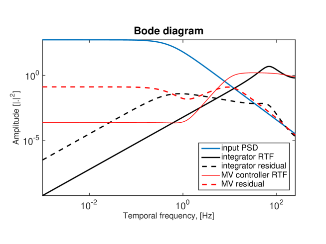
Figure 2: (Colour on-line) Example input disturbance and rejection transfer functions for the integrator and LQG controllers.

Salient features are:

• The optimal controller rejection is proportional to 40dB/dec whereas the integrator is only 20db/dec. This is a tunable parameter that depends on the model order to achieve 20dB/dec $\times$ model-order.

• There is a knee at low frequencies such that the residual PSD is as flat as possible. This depends on the parameters $\{a,b,\cdots\}$ of the model

2.3 Multi-mode case

From the results above in the mono-mode, scalar case, we can extend the reasoning to a larger set of modes. Initial results were developed in [33, 11] and later extended by [34, 24, 35] using a Zernike modal basis[36]. Of particular insight is the work by Conan [37] that covers in greater detail than I could possibly do here the application to the multiple-input, multiple-output (MIMO) case. From the observation that the LQG controller provides better rejection for every mode, one can either

1. improve the performance for a given sampling frequency or

2. relax the sampling frequency, thus integrate longer whilst keeping a performance not worst than the integrator.

Implementations on systems beyond just tip-tilt modes showed promising results on Canary [3] and Raven [4].

2.4 Vibrations

Vibrations are considered a major source of disturbance affecting almost all observatories around the globe [38]. Most remarkably, the LQG has been successfully applied to vibration rejection on SPHERE [39] and GPI [40] using formalism developed in [41, 42, 43].

A continuous-time model is provided in [44] which is quite convenient for LGS-based tomographic systems where the low-order modes are corrected separately and potentially at lower frame rates to allow for improved sky-coverage [19, 20].

In practice the vibration model is concatenated with that in Eq. (17) in order to obtain a notch at the vibration central frequencies.

2.5 From 8 m to 40 m class telescopes

The optimal control features are particularly useful on 40 m class telescopes, particularly the low-order modes. Since the lowest spatial frequency is $\propto 1/D$, low-order modes will carry lot more disturbance $\propto(D/r_{0})^{5/3}$ [37]. This in turn indicates that we need a means to adjust the rejection at very low frequencies along the lines presented in Fig. 2. Conan et al (2011)[37] provide a full account of the advantages of optimal control on 40 m class telescopes.

2.6 The MMSE as a degraded solution of the optimal control

It has been early recognised that the minimum-mean squared error solution to the (spatial) mode estimation can be obtained seamlessly from the LQG solution. This is achieved by noting that under a static assumption (i.e. no temporal delays, memoryless model) then $\mathcal{A}=\mathbf{I}$, i.e. ${\mathbf{\psi}}_{k+1}={\mathbf{\psi}}_{k}$ the conditional expectation $\widehat{{\mathbf{x}}}_{k|k-1}=0$. The estimation error covariance matrix becomes in this case $\mathbf{\Sigma}_{\infty}=\mathbf{\Sigma}_{\mathbf{\psi}}$ the uncorrected phase covariance matrix leading to

$$\widehat{{\mathbf{x}}}_{k}=\mathbf{H}_{\infty}({\mathbf{s}}_{k}+\mathcal{D}_{\mathsf{tur}}{\mathbf{u}}_{k-d})$$ (20)

and as before

$${\mathbf{u}}_{k}=\mathbf{F}\widehat{{\mathbf{x}}}^{\prime}_{k|k}=\mathbf{F}\widehat{{\mathbf{\psi}}}_{k|k}$$ (21)

The term ${\mathbf{s}}_{k}+\mathcal{D}{\mathbf{u}}_{k-d}$ represents the so-called pseudo open-loop slopes, i.e. the solution obtained although specified for closed-loop systems makes ”as if” it were in open-loop. If instead we were working directly in open loop, then $\mathcal{D}_{\mathsf{tur}}=0$ and the same structure is kept. This is a remarkable feature of the LQG that ultimately stems from the separation principle.

Since the intrinsic model of the MMSE solution assumes intrinsically $\mathcal{A}_{\mathsf{tur}}=\mathbf{I}$ this model is unstable (energy unbound) representative of a random walk. Adaptation of the MMSE to the closed-loop case has been proposed in [45] as a pseudo open-loop control (POLC) or in [46] – neither inspired in Eq. (20) –, ensuring on the one hand that the MMSE solution is used (mainly for computational reasons) and that the solution is stable, although sub-optimal. POLC solutions are the baseline for the AO systems of all giant telescopes, both implementing laser-tomography (as is the case of the ELT and GMT) or multi-conjugation (the case of TMT and the ELT).

2.7 Robustness and model identification

Robustness to changing observing conditions is an item that deserves special care. Identification of models [30] and adaptation to unstationary conditions can be found in [47]. Recent work is reported in [48].

3 Optimal control in large scale AO

Although theoretically very appealing, optimal control has several drawbacks for real-time environments:

• The filter is recursive meaning that the (k – 1) estimate is needed to update the state. This is by no means fundamentally different from integrator-based update equations coupled or not to pseudo-open-loop measurements calculation;

• The gain computation commonly involves the inversion of state-sized matrix equation which by itself is unappealing;

• The state has usually a much higher dimension than the input or output vectors.

3.1 Wide-field AO systems

Several adaptations to large scale AO systems have been pursued over the years, in particular wide-field AO. It has been observed – and extensively used for modelling purposes – that the main operations involved in the forward process are, or can reasonably be approximated by, circular convolutions with localized kernels. Here we talk about propagation in weak-turbulence (geometric optics applies, otherwise Fourier optics needed), angular shifts that convert to spatial shifts through easy-to-grasp geometric transformations, temporal shifts which convert correspondingly to spatial shifts on account of the frozen-flow hypothesis and finally, the critical point for modellers, describing the wave-front sensor (WFS) through filtering operations.

Calculations in the spatial Fourier domain are particularly suitable for the Fourier-transformed bidimensional operators become diagonal. The problem with this approach is that of the spatial invariance of the operators – it is only an approximation due to the fact that all telescope have finite apertures. This leads to boundary issues (so common in many other fields of physics and engineering) and to circularity concerns. For instance, although the covariance matrices appearing in the formulations admit a quasi-diagonal representation in the spatial Fourier-domain, the matrices are instead Toeplitz with Toeplitz blocks and not circulant with circulant blocks. Rodoplhe Conan points out the exact multiplication of a vector by a Toeplitz matrix in the Fourier-domain [49] a work later extended in [50].

On the same vein we also note the annular shapes of telescope apertures are not adapted to the use of bi-dimensional Fourier transforms. As argued elsewhere, the Fourier modes are shown to be the eigenmodes of the bi-harmonic equation on a rectangular domain. For annular domains the use of disk-harmonic functions would therefore seem more suited, as they are in turn shown to be the eigenmodes of the bi-harmonic equation on a circle.

The localised kernels mean in turn that sparse techniques are in principle applicable giving rise to approximate models with a reduced number of non-zero entries [51].

In the recent past several research papers on the optimisation of Kalman filters were published. The ideas therein can somehow arbitrarily be categorized as follows, involving both runtime and off-line optimization:

• For the main flavours of AO – single-conjugate (SCAO), ground-layer (GLAO), multi-object (MOAO), laser-tomography (LTAO) systems –, the need to estimate only a pupil-plane wave-front (possibly averaged over several optimization directions) means that the explicit estimation of layered wave-front profiles can be circumvented leading to considerable computational savings. Resorting to a pixelated description of the wave-fronts (customarily a zonal basis) all the matrices in the spate-space model are sparse but the state transition. Calling for the quasi-Markovianity of the model, reasonable approximations can be found of which bilinear spline phase-shifting operators are a good proxy [35].

• Using directly the complex-exponential basis. In this case the modes are temporally and statistically independent (reasonable approximation) which means calculations can be done on a mode-per-mode basis – we’re thus under a distributed control framework [52]. It goes without saying that the gain is also computed in such parallel fashion which is chiefly important for off-line but also real-time operations, boiling down to localised convolutions. We note also that, unlike in the previous item, the state-transition matrix is (complex) diagonal. Each entry is a phasor to produce a spatial shift of every mode, mimicking thus wind-blown wave-fronts translating across the pupil [53, 15].

• Using sparse approximations to the discrete-time Riccati equation (DARE) solution and apply the gain by formulating the result as the search for the unknowns x in the Ax = b linear system of equations [5].

• Doing a Taylor expansion of the DARE to break the algebraic nature of the Riccati equation, solving for it using a closed-form equation [6].

• Applying the finite-horizon Kalman filter. Instead of using the infinite-horizon steady-state Kalman gain, fixing a sliding, finite-horizon with h steps, and then use at any time step k only the measurements from ($k–1$) to ($k–h$) to get an estimate. In such case the problem can be cast as a vector-matrix multiplication (VMM). [7]

3.2 High-contrast AO systems

For high-contrast AO systems, the focus is more on optical performance than beating computational constraints which, for this class of systems, are less of a problem.

The use of predictive control bears the hope of considerably reducing the servo-lag error. The latter manifest itself as a butterfly-like pattern close to the post-coronagraphic PSF core, much reducing the achievable contrast [54]. The use of the complex exponential basis is particularly adapted on account of the post-coronagraphic PSF and residual error PSD with speckles directly obtained as a scaled version of the PSD [53, 15, 55]. Although the models are suitable, identification of the correct parameters and robustness in changing observing conditions are the main limitations to the implementation of predictive control on-sky.

4 SUMMARY

Optimal dynamical control has a handful of very welcome advantages, including

• Common and non-common path optical aberrations can be directly modelled in the state-space

• Vibrations can be straightforwardly fed-in

• The gains are analytically found, no need to cumbersome dichotomy search routines

• Dealing with the open or close loop nature of the loops is transparent – pseudo open-loop measurements are obtained at each update step in the latter case when manipulating the Kalman equations

• The spatio-temporal nature of the AO optimization problem, i.e. the temporal dynamics of the loop is factored in analytically and not following ad-hoc techniques.

• The estimation and prediction error variances are found directly from the filter optimization.

• General-case scenario: optical performance is considerably enhanced

Yet, it also faces several challenges. Of main concern is the computational complexity associated with finding the optimal gain matrices on large scale AO systems, specially tomographic AO using several wave-front sensor probes.

- [1] Roddier, F., [Adaptive Optics in Astronomy ], Cambridge University Press, New York (1999).
- [2] J.W.Hardy, [Adaptive Optics for Astronomical Telescopes ], Oxford, New York (1998).
- [3] Sivo, G., Kulcsár, C., Conan, J.-M., Raynaud, H.-F., Éric Gendron, Basden, A., Vidal, F., Morris, T., Meimon, S., Petit, C., Gratadour, D., Martin, O., Hubert, Z., Sevin, A., Perret, D., Chemla, F., Rousset, G., Dipper, N., Talbot, G., Younger, E., Myers, R., Henry, D., Todd, S., Atkinson, D., Dickson, C., and Longmore, A., “First on-sky scao validation of full LQG control with vibration mitigation on the canary pathfinder,” Opt. Express 22, 23565–23591 (Sep 2014).
- [4] Lardière, O., Andersen, D., Blain, C., Bradley, C., Gamroth, D., Jackson, K., Lach, P., Nash, R., Venn, K., Véran, J.-P., Correia, C., Oya, S., Hayano, Y., Terada, H., Ono, Y., and Akiyama, M., “Multi-object adaptive optics on-sky results with raven,” Proc. SPIE 9148, 91481G–91481G–14 (2014).
- [5] Correia, C., Conan, J.-M., Kulcsár, C., Raynaud, H.-F., and Petit, C., “Adapting optimal LQG methods to ELT-sized AO systems,” in [1st AO4ELT Conference - Adaptative Optics for Extremely Large Telescopes proceedings ], Y. Clénet, J.-M. Conan, T. F. and Rousset, G., eds., AO4ELT , EDP Sciences (jun 2009).
- [6] Massioni, P., Kulcsár, C., Raynaud, H.-F., and Conan, J.-M., “Fast computation of an optimal controller for large-scale adaptive optics,” J. Opt. Soc. Am. A 28, 2298–2309 (Nov 2011).
- [7] Massioni, P. and Di Loreto, M., “Fast finite-horizon kalman filter in wavefront estimation for adaptive optics,” in [European Control Conference ], ECC, ed. (2014).
- [8] Anderson, B. D. O. and Moore, J. B., [Optimal Control, Linear Quadratic Methods ], Dover Publications Inc. (1995).
- [9] Gendron, E. and Léna, P., “Astronomical adaptive optics I: Modal control optimization,” Astronomy and Astrophysics 291, 337–347 (1994).
- [10] Dessenne, C., Madec, P.-Y., and Rousset, G., “Optimization of a predictive controller for closed-loop adaptive optics,” Appl. Opt. 37, 4623–4633 (1998).
- [11] Kulcsár, C., Raynaud, H.-F., Petit, C., Conan, J.-M., and de Lesegno, P. V., “Optimal control, observers and integrators in adaptive optics,” Opt. Express 14(17), 7464–7476 (2006).
- [12] Ellerbroek, B. L., “Linear systems modeling of adaptive optics in the spatial-frequency domain,” J. Opt. Soc. Am. A 22, 310–322 (Feb 2005).
- [13] Rigaut, F. J., Véran, J.-P., and Lai, O., “Analytical model for Shack-Hartmann-based adaptive optics systems,” in [Proc. of the SPIE ], Bonaccini, D. and Tyson, R. K., eds., Adaptive Optical System Technologies 3353(1), 1038–1048, SPIE (1998).
- [14] Jolissaint, L., “Synthetic modeling of astronomical closed loop adaptive optics,” Journal of the European Optical Society - Rapid publications, 5, 10055 5 (Nov. 2010).
- [15] Correia, C. M., “Temporally filtered wiener phase reconstruction in astronomical adaptive optics from slope data,” JOSA A submitted (2017).
- [16] Suzanne K. Ramsay, Mark M. Casali, N. H. M. K.-P. H.-U. K. J.-L. L. J. S., “A roadmap for the e-elt instrument suite,” Proc.SPIE 8446, 8446 – 8446 – 8 (2013).
- [17] Antonin H. Bouchez, D. Scott Acton, R. B. R. C.-B. E.-S. E. J. F. D. G. B. A. M. E. P. F. S. G. T. M. A. v. D., “The giant magellan telescope adaptive optics program,” Proc.SPIE 9148, 9148 – 9148 – 19 (2014).
- [18] C. Boyer, B. E., “Adaptive optics program update at tmt,” Proc.SPIE 9909, 9909 – 9909 – 14 (2016).
- [19] Correia, C., Véran, J.-P., Herriot, G., Ellerbroek, B., Wang, L., and Gilles, L., “Increased sky coverage with optimal correction of tilt and tilt-anisoplanatism modes in laser-guide-star multiconjugate adaptive optics,” J. Opt. Soc. Am. A 30, 604–615 (Apr 2013).
- [20] Wang, L., Gilles, L., Ellerbroek, B., and Correia, C., “Physical optics modeling of sky coverage for tmt nfiraos with advanced lqg controller,” Proc. SPIE 9148, 91482J–91482J–10 (2014).
- [21] Carlos M. Correia, Benoit Neichel, J.-M. C. C. P.-J.-F. S. T. F. J. D. R. V. N. T., “Natural guide-star processing for wide-field laser-assisted ao systems,” Proc.SPIE 9909, 9909 – 9909 – 13 (2016).
- [22] Herrmann, J., “Phase variance and Strehl ratio in adaptive optics.,” J. Opt. Soc. Am. A 9, 2257–2258 (Dec. 1992).
- [23] Correia, C., Raynaud, H.-F., Kulcsár, C., and Conan, J.-M., “On the optimal reconstruction and control of adaptive optical systems with mirror dynamics,” J. Opt. Soc. Am. A 27, 333–349 (Feb. 2010).
- [24] Correia, C., Design of high-performance control laws for very/extremely large astronomical telescopes, PhD thesis, E. D. Galilée, Univ. Paris XIII (Mar 2010).
- [25] Looze, D. P., “Discrete-time model of an adaptive optics systems,” J. Opt. Soc. Am. A 24, 2850–+ (2007).
- [26] Kulcsár, C., Raynaud, H.-F., Petit, C., and Conan, J.-M., “Minimum variance prediction and control for adaptive optics,” Automatica 48(9), 1939 – 1954 (2012).
- [27] Anderson, B. D. O. and Moore, J. B., [Optimal Filtering ], Dover Publications Inc. (1995).
- [28] Gilles, L., Massioni, P., Kulcsár, C., Raynaud, H.-F., and Ellerbroek, B., “Distributed Kalman filtering compared to Fourier domain preconditioned conjugate gradient for laser guide star tomography on extremely large telescopes,” J. Opt. Soc. Am. A 30, 898 (May 2013).
- [29] Oppenheim, A. V. and Willsky, A. S., [Signals & Systems ], Prentice-Hall,Inc., 2nd ed. (1997).
- [30] Hinnen, K., Verhaegen, M., and Doelman, N., “Exploiting the spatiotemporal correlation in adaptive optics using data-driven H2-optimal control,” J. Opt. Soc. Am. A 24, 1714–1725 (June 2007).
- [31] Conan, J.-M., Rousset, G., and Madec, P.-Y., “Wave-front temporal spectra in high-resolution imaging through turbulence,” J. Opt. Soc. Am. A 12, 1559–1570 (1995).
- [32] Conan, R. and Correia, C., “Object-oriented matlab adaptive optics toolbox,” in [Proc. of the SPIE ], 9148, 91486C–91486C–17 (2014).
- [33] Le Roux, B., Conan, J.-M., Kulcsár, C., Raynaud, H.-F., Mugnier, L. M., and Fusco, T., “Optimal control law for classical and multiconjugate adaptive optics,” J. Opt. Soc. Am. A 21, 1261–1276 (2004).
- [34] Petit, C., Conan, J.-M., Kulcsár, C., and Raynaud, H.-F., “Linear quadratic gaussian control for adaptive optics and multiconjugate adaptive optics: experimental and numerical analysis,” J. Opt. Soc. Am. A 26(6), 1307–1325 (2009).
- [35] Correia, C. M., Jackson, K., Véran, J.-P., Andersen, D., Lardière, O., and Bradley, C., “Spatio-angular minimum-variance tomographic controller for multi-object adaptive-optics systems,” Appl. Opt. 54, 5281–5290 (Jun 2015).
- [36] Noll, R. J., “Zernike polynomials and atmospheric turbulence,” J. Opt. Soc. Am. A 66, 207–211 (1976).
- [37] Conan, J. M., Raynaud, H. F., Kulcsár, C., and Meimon, S., “Are integral controllers adapted to the new era of ELT adaptive optics?,” in [Second International Conference on Adaptive Optics for Extremely Large Telescopes. Online at ¡A href=”http://ao4elt2.lesia.obspm.fr”¿http://ao4elt2.lesia.obspm.fr¡/A ], 57 (Sept. 2011).
- [38] Caroline Kulcs r, Gaetano Sivo, H.-F. R. B. N. F. R.-J. C. A. G. C. C. J.-P. V. E. G. F. V. G. R. T. M. S. E. F. Q.-P. G. A. E. F. L. P. R. C. R. M. O. G. F. M. S. M. J.-M. C., “Vibrations in ao control: a short analysis of on-sky data around the world,” Proc.SPIE 8447, 8447 – 8447 – 14 (2012).
- [39] Fusco, T., Sauvage, J. F., Mouillet, D., Costille, A., Petit, C., Beuzit, J. L., Dohlen, K., Milli, J., Girard, J., Kasper, M., Vigan, A., Suarez, M., Soenke, C., Downing, M., N’Diaye, M., Baudoz, P., Sevin, A., Baruffolo, A., Schmid, H. M., Salasnich, B., Hugot, E., and Hubin, N., “SAXO, the SPHERE extreme AO system: on-sky final performance and future improvements,” in [Adaptive Optics Systems V ], 9909, 99090U (July 2016).
- [40] Poyneer, L. A., De Rosa, R. J., Macintosh, B., Palmer, D. W., Perrin, M. D., Sadakuni, N., Savransky, D., Bauman, B., Cardwell, A., Chilcote, J. K., Dillon, D., Gavel, D., Goodsell, S. J., Hartung, M., Hibon, P., Rantakyrö, F. T., Thomas, S., and Veran, J.-P., “On-sky performance during verification and commissioning of the Gemini Planet Imager’s adaptive optics system,” in [Adaptive Optics Systems IV ], 9148, 91480K (July 2014).
- [41] Petit, C., Conan, J.-M., Kulcsár, C., Raynaud, H.-F., and Fusco, T., “First laboratory validation of vibration filtering with LQG control law for adaptive optics,” Opt. Express 16(1), 87–97 (2008).
- [42] Meimon, S., Petit, C., Fusco, T., and Kulcsar, C., “Tip–tilt disturbance model identification for Kalman-based control scheme: application to XAO and ELT systems,” J. Opt. Soc. Am. A 27(11), A122–A132 (2010).
- [43] Poyneer, L. A. and Véran, J.-P., “Kalman filtering to suppress spurious signals in adaptive optics control,” J. Opt. Soc. Am. A 27(11), A223–A234 (2010).
- [44] Correia, C., Véran, J.-P., and Herriot, G., “Advanced vibration suppression algorithms in adaptive optics systems,” J. Opt. Soc. Am. A 29, 185–194 (Mar 2012).
- [45] Gilles, L., “Closed-loop stability and performance analysis of least-squares and minimum-variance control algorithms for multiconjugate adaptive optics,” Appl. Opt. 44, 993–1002 (feb 2005).
- [46] Béchet, C., Tallon, M., Tallon-Bosc, I., Thiébaut, E., Louarn, M. L., and Clare, R. M., “Optimal reconstruction for closed-loop ground-layer adaptive optics with elongated spots,” J. Opt. Soc. Am. A 27(11), A1–A8 (2010).
- [47] Doelman, N. and Osborn, J., “Modelling and prediction of non-stationary optical turbulence behaviour,” in [Adaptive Optics Systems V ], 9909, 99091M (July 2016).
- [48] van Kooten, M. and Doelman, N., “Implications for contrast as a result of the wind vector and non- stationary turbulence,” in [Proc. of the SPIE ], (2018).
- [49] Conan, R., “Fast iterative optimal estimation of turbulence wavefronts with recursive block toeplitz covariance matrix,” Proc. SPIE 9148, 91480R–91480R–15 (2014).
- [50] Ono, Y. H., Correia, C., Conan, R., Blanco, L., Neichel, B., and Fusco, T., “Fast iterative tomographic wavefront estimation with recursive toeplitz reconstructor structure for large-scale systems,” J. Opt. Soc. Am. A 35, 1330–1345 (Aug 2018).
- [51] Ellerbroek, B. L., Gilles, L., and Vogel, C. R., “A computationally efficient wavefront reconstructor for simulation of multi-conjugate adaptive optics on giant telescopes,” in [Adaptive Optical System Technologies II. Edited by Wizinowich, Peter L.; Bonaccini, Domenico. Proc. of the SPIE, Volume 4839, pp. 989-1000 (2003). ], 4839, 989–1000 (2003).
- [52] Massioni, P., Gilles, L., and Ellerbroek, B., “Adaptive distributed kalman filtering with wind estimation for astronomical adaptive optics,” J. Opt. Soc. Am. A 32, 2353–2364 (Dec 2015).
- [53] Poyneer, L. and Véran, J.-P., “Predictive wavefront control for adaptive optics with arbitrary control loop delays,” J. Opt. Soc. Am. A 25(7), 1486–1496 (2008).
- [54] Guyon, O. and Males, J., “Adaptive Optics Predictive Control with Empirical Orthogonal Functions (EOFs),” ArXiv e-prints , arXiv:1707.00570 (July 2017).
- [55] Jared R. Males, O. G., “Ground-based adaptive optics coronagraphic performance under closed-loop predictive control,” Journal of Astronomical Telescopes, Instruments, and Systems 4, 4 – 4 – 21 (2018).