The impact of AGN on stellar kinematics and orbits in simulated massive galaxies

Abstract

We present a series of 20 cosmological zoom simulations of the formation of massive galaxies with and without a model for AGN feedback. Differences in stellar population and kinematic properties are evaluated by constructing mock integral field unit (IFU) maps. The impact of the AGN is weak at high redshift when all systems are mostly fast rotating and disc-like. After $z\sim 1$ the AGN simulations result in lower mass, older, less metal rich and slower rotating systems with less disky isophotes - in general agreement with observations. Two-dimensional kinematic maps of in-situ and accreted stars show that these differences result from reduced in-situ star formation due to AGN feedback. A full analysis of stellar orbits indicates that galaxies simulated with AGN are typically more triaxial and have higher fractions of x-tubes and box orbits and lower fractions of z-tubes. This trend can also be explained by reduced late in-situ star formation. We introduce a global parameter, $\xi_{3}$, to characterise the anti-correlation between the third-order kinematic moment $h_{3}$ and the line-of-sight velocity ($v_{los}/\sigma$), and compare to ATLAS^3D observations. The kinematic asymmetry parameter $\xi_{3}$ might be a useful diagnostic for large integral field surveys as it is a kinematic indicator for intrinsic shape and orbital content.

1 Introduction

The connection between active galactic nuclei (AGN) and their host galaxies has been subject of research for more than two decades. Soon after the discovery of super-massive black holes (SMBH) in the centres of early-type galaxies, correlations have been found between their mass and galactic properties such as galactic bulge mass and velocity dispersion (Dressler, 1989; Kormendy, 1993; Gebhardt et al., 2000). This connection has been in the focus of theoretical work with the conclusion that the energy feedback from accreting black holes could be necessary to reproduce these scaling relations as well as the correct masses and abundances of early-type galaxies in cosmological simulations (see e.g. Croton et al., 2006; Schaye et al., 2015; Vogelsberger et al., 2014 and reviews by Kormendy & Ho (2013), Somerville & Davé (2015) and Naab & Ostriker (2017)). However, the impact of AGN might go beyond affecting global properties. The cosmological simulations of Choi et al. (2015); Choi et al. (2017) showed that in low-redshift galaxies the fraction of stars that form in-situ is much lower when including AGN feedback. This has strong repercussions on the morphological and kinematic properties of these galaxies: in-situ formed stars tend to form orderly-rotating discs, while stars which are accreted from other galaxies form round dispersion-supported systems. Because of this connection, many studies attributed the difference in properties of present-day galaxies to stellar origins. The more massive early-type galaxies, whose stellar component has been for a significant part accreted, tend to have smaller angular momentum (Emsellem et al., 2011) and more complex kinematics (Krajnović et al., 2011), while intermediate and low-mass galaxies, which have formed most of their stars in-situ, are simple fast-rotating systems (see Cappellari (2016) for a review). Naab et al. (2014) and Röttgers et al. (2014) linked the present-day kinematics of simulated galaxies to the type of galaxy mergers they experienced during their formation: minor or major, and with or without gas. This picture would however be incomplete without including AGN feedback. Dubois et al. (2016) and Penoyre et al. (2017a) showed that only with AGN feedback they were able to obtain realistic abundances of slow-rotating systems in cosmological simulations. In this paper we analyse a small sample of high-resolution ‘zoom’ simulations (see Figure 1) for a more in-depth look at the impact of AGN feedback on the kinematic and stellar-population properties of galaxies, but also extending the analysis to higher-order kinematics and orbital structure. We compare our simulated galaxies to observations by mocking the images produced by integral field unit (IFU) spectrographs. These instruments collect a spectrum for each of their spatial pixels, so that one can observe the spatial distribution of spectrum-derived quantities, such as line-of-sight velocity, metallicity and age. Recently a number of large galaxy surveys have been performed with IFU spectrographs, such as MaNGA (Bundy et al., 2015), SAMI (Croom et al., 2012) and CALIFA (Sánchez et al., 2012), resulting in the mapping of thousands of galaxies. The MUSE spectrograph (Bacon et al., 2010) also delivered detailed 2D maps of galactic properties (e.g., Emsellem et al., 2014, Krajnović et al., 2018), including at high redshift (Guérou et al., 2016). For the study of AGN feedback, this means that there is a huge library of data that can be used to look for signatures of the effect of AGNs, and in this paper we want to understand the nature of generic signatures through cosmological simulations. We do this by running each of our simulations twice, once with and once without our AGN feedback implementation, in order to find and analyse the differences between the two cases. In Section 2 we present the set of cosmological simulations analysed in this paper. In Section 3 we describe how our mock observational maps are created, and how the other values we present are calculated. In Section 4 we look at the effect of AGN feedback on one exemplary simulated galaxy, through our mock integral field maps. In Section 5 we analyse the full simulation sample, to get an idea of the general impact of AGN feedback. In Section 6 we discuss and summarise our conclusions.

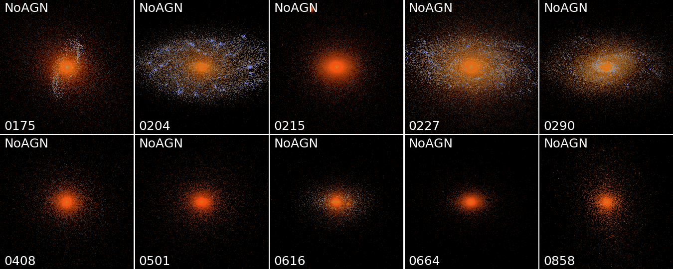
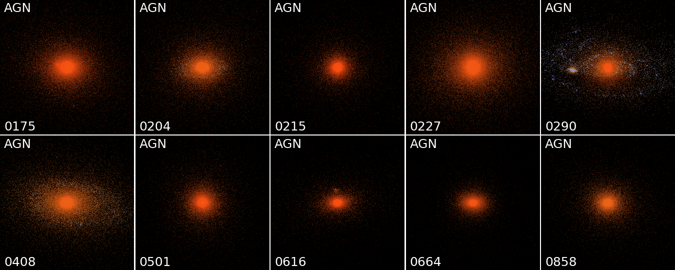
Figure 1: Mock luminosity images of our sample of simulated galaxies, run without (top two rows) and with (bottom two rows) AGN feedback. All galaxies are viewed at an angle of 30 degrees. Stars are colour-coded by V-band weighted age based on Bruzual & Charlot (2003). Many of the galaxies simulated without AGN feedback show the presence of young stellar discs, despite being massive ellipticals.

2 Simulation details

2.1 Cosmological ‘zoom’ simulations

In this work we analyse a set of twenty prototypical cosmological zoom simulations of massive galaxies for the impact of feedback from accreting super-massive black holes. Each initial condition is simulated once with and once without the AGN feedback model. Throughout the paper the two cases will be labelled as AGN and NoAGN. The initial conditions for the simulations were constructed from a $(100\,{\rm Mpc})^{3}$ dark matter only simulation with a WMAP3 cosmology (Spergel et al., 2007): $h=0.72,\Omega_{\rm b}=0.044,\Omega_{\rm dm}=0.216,\Omega_{\Lambda}=0.74,\sigma_{\rm 8}=0.77,n_{\rm s}=0.95$ . All details on the construction of the zoom initial conditions are presented in Oser et al. (2010, 2012). The same initial conditions were used in e.g. Naab et al., 2014 and Hirschmann et al., 2012; Hirschmann et al., 2013; Naab et al., 2014 and Hirschmann et al., 2017, but here we simulate at higher resolution. Dark matter particles have a mass of $m_{p}=3.62\cdot 10^{6}\,M_{\odot}\,h^{-1}$ and gas particles initially have mass of $m_{p}=7.37\cdot 10^{5}M_{\odot}\,h^{-1}$. The simulations are run from $z=43$ to $z=0$ with gravitational softening lengths of $0.2\,\rm kpc$ for gas, star and black hole particles and $0.45\,\rm kpc$ for dark matter particles at the highest resolution level.
The simulation code is the same as the one used in Hirschmann et al. (2017). We used an improved version of GADGET3 (Springel, 2005), SPHgal, which overcomes the numerical limitations of the classic smoothed particle hydrodynamics (SPH) implementation. All details of SPHgal are given in Hu et al. (2014). We use a pressure-entropy SPH formulation, a Wendland $C^{4}$ kernel with 200 neighbouring particles, artificial thermal conductivity and an improved modelling of artificial viscosity.

2.1.1 Star formation and feedback

The simulation code includes a model for the formation of stellar populations from gas particles, representing star formation and for feedback. The stellar populations provide thermal and kinetic feedback as well as metals to the inter-stellar medium. The chemical enrichment was originally described by Scannapieco et al. (2005, 2006) and later improved by Aumer et al. (2013) and Núñez et al. (2017) with an updated feedback model. Gas particles are stochastically converted into star particles depending on the density of the gas, in a way that reproduces the Kennicutt-Schmidt relation (Kennicutt, 1998). To be eligible for conversion into stars, SPH particles need to have a temperature lower than $12,000\,\rm K$ and a density higher than $1.94\times 10^{23}\,\rm g\,cm^{-3}$. The probability for conversion during a time step of $\delta t$ is $1-e^{-p_{\rm SF}}$, where:

$$p_{\rm SF}=\epsilon_{\rm SFR}\,\sqrt{4\,\pi\,G\,\rho}\,\delta t$$ (1)

and $\epsilon_{\rm SFR}$ is set to $0.02$ (see e.g. Springel, 2000). The newly-created star particles are then treated as collisionless. Each particle represents a single stellar population assuming a Kroupa (2001) initial mass function, with a given age and the metallicity of the original gas particle. This stellar population then exerts feedback to the surrounding gas. This takes the form of type Ia and II supernovae and of winds from asymptotic giant branch (AGB) stars. Supernovae Type II happen at a given time $\tau_{SNII}=3\,\rm Myr$ after the creation of the star particles, where $\tau_{SNII}$. This is on the short end of the typical delay time distributions for supernovae type II. Supernovae type Ia and AGB winds are added continuously every $50\rm Myr$ after the star particle creation. Each event provides momentum and thermal energy to the surrounding gas. The total feedback energy is given by:

$$E=\frac{1}{2}\,m_{\rm ejected}\,v_{\rm out}^{2},$$ (2)

where $m_{\rm ejected}$ is the mass ejected by the stellar population and $v_{\rm out}$ is the assumed ejecta velocity. These are determined depending on the mass, age and metallicity of the particle and on the type of event. We assume $v_{\rm out}=4500kms^{-1}$ for SNIa and SNII and $v_{\rm out}=10kms^{-1}$ for AGB stars. The ejecta mass is taken from Woosley & Weaver (1995) for SNII and from Iwamoto et al. (1999) for SNIa. This energy and mass is then added to the surrounding gas both as thermal (heating) and as momentum feedback (pushing). The relative fraction depends on the density and distance between the supernova-undergoing stellar particle and the 10 neighbouring gas particles, mimicking the evolution of blast waves (a simplified version of the three-phase model adopted in Núñez et al. (2017); see Hirschmann et al. (2017)). The feedback events also distribute metals to the surrounding gas. Eleven elements are tracked for every gas and star particle (H, He, C, N, O, Ne, Mg, Si, S, Ca, and Fe), and their abundances are used to compute the cooling rate of the gas with the yields from Karakas (2010), Iwamoto et al. (1999) and Woosley & Weaver (1995) for AGB winds and supernovae type Ia and II, respectively. All details can be found in Aumer et al. (2013), Aumer et al. (2014), and Núñez et al. (2017).

2.1.2 AGN feedback

AGN feedback is represented through the model developed by Choi et al. (2012) and used in Choi et al. (2014, 2015); Choi et al. (2017). This model includes both a radiative and a kinetic (wind) component (see Naab & Ostriker, 2017 for a discussion of alternative numerical implementations). For massive galaxies this results in efficient and realistic suppression of star formation, as well as good agreement with the observed black hole mass relations and X-ray luminosities (Choi et al., 2015; Eisenreich et al., 2017). Here we summarise the most important elements used for this study. Black holes are first seeded at the centre of halos exceeding a mass of $10^{11}\,M_{\odot}$, with an initial mass of $M_{\mathrm{BH}}=10^{5}\,M_{\odot}$. They can then grow either by merging with other black hole particles or by accreting neighbouring gas particles according to a modified Bondi-Hoyle-Lyttleton (Hoyle & Lyttleton, 1939,
Bondi & Hoyle, 1944, Bondi, 1952) accretion rate:

$$\dot{M}_{\rm BHL}=\left<\frac{4\,\pi\,G^{2}\,M_{\rm BH}^{2}\,\rho}{(c_{s}^{2}+v^{2})^{3/2}}\right>,$$ (3)

where $M_{\rm BH}$ is the mass of the super massive black hole, $\rho$ is the density of the gas, $v$ its relative speed and $c_{s}$ is its speed of sound. The angle brackets indicate SPH kernel averaging. Of the gas particles which could be accreted, 90% are re-emitted as a wind parallel to the angular momentum of the gas next to the black hole (see Ostriker et al., 2010). This simulates the broad-line winds commonly emitted by AGN (de Kool et al., 2001; Somerville & Davé, 2015; Naab & Ostriker, 2017). The remaining 10% are accreted, increasing the mass of the black hole particle. The model also includes radiative feedback, in two forms. There is an Eddington radiation pressure force, which depends on the accretion rate and represents low energy photons providing momentum to the gas isotropically. We are also representing the higher energy X-ray photons, using the formulae from Sazonov et al. (2005) for Compton scattering. This component provides both momentum and thermal energy to the gas. As in Hirschmann et al. (2017), our simulation code differs from the one used in Choi et al. (2017) in not including metallicity-dependent heating, which was shown to have negligible impact(Choi et al., 2017).

3 Analysis methods

3.1 Voronoi-binned kinematic maps

We study our simulations by analysing a series of mock integral field unit (IFU) maps (e.g. Cappellari et al., 2011a) of the kinematics, metallicities and ages of the stellar populations of the simulated galaxies. These maps are constructed with a Python code developed for this work, following the analysis presented in Jesseit et al. (2007, 2009); Röttgers et al. (2014); Naab et al. (2014). The code is included in the publicly available PYGAD analysis package . Positions and velocities of the simulated galaxies are centred on the densest nuclear regions using a shrinking sphere technique on the stellar component. In the AGN simulations we centre the galaxies on their central super-massive black hole particles, which we define as the most massive black hole particle within $1\rm kpc$ of the stellar density centre. We then calculate the eigenvectors of the reduced inertia tensor (Bailin & Steinmetz, 2005) of all stellar particles within 10 % of the virial radius, and use them to align the galaxies’ principal axes with the coordinate systems, such that the x-axis is the long axis and the z-axis is the short axis. To mimic seeing effects, each star particle in the simulation is split into 60 ‘pseudo-particles’, which keep the same velocity as the original particle and the positions are distributed according to a Gaussian with $\sigma=0.2\,\rm kpc$ centred on the original position of the particle (see Naab et al., 2014). In projection, the pseudo-particles are mapped onto a regular two-dimensional grid, with pixel size $0.1\,\rm kpc$ (at $z=0$). Adjacent bins of this grid are then joined so that each resulting spaxel has a similar signal-to-noise ratio. We do this using the Voronoi tessellation method presented in Cappellari & Copin (2003). For the maps presented in this paper, the target signal-to-noise level of the spaxels has been set such that each of them contains $25000$ pseudo-particles ($\sim 400$ regular particles). This ensures good statistics and results in maps similar to the ones from modern integral field surveys. The Voronoi grid is then used to construct the plots of stellar kinematics, metallicity and age shown in this paper. For the age and metallicity maps, the value of every spaxel is calculated through a mass-weighted sample average. For the kinematic maps, we construct a histogram of the line-of-sight (LOS) velocity distribution of each spaxel, with the bin size determined by the Freedman & Diaconis (1981) rule. We then follow the classic approach of van der Marel & Franx (1993); Gerhard (1993) and fit the LOS velocity histogram with a Gauss-Hermite function:

$$f(V)=I_{0}\,e^{-y^{2}/2}(1+h_{3}\,H_{3}(y)+h_{4}\,H_{4}(y))$$ (4)

where $y=(V-V_{\rm avg})/\sigma$ and $H_{3}$ and $H_{4}$ are the Hermite polynomials of third and fourth order:

$$H_{3}(y)=(2\,\sqrt{2}\,y^{3}-3\,\sqrt{2}\,y)/\sqrt{6}$$ (5)

$$H_{4}(y)=(4\,y^{4}-12\,y^{2}+3)/\sqrt{24}$$ (6)

The four fitting parameters $V_{\rm avg}$ (average velocity), $\sigma$ (velocity dispersion), $h_{3}$ (skewness of the distribution), $h_{4}$ (kurtosis of the distribution) are the ones plotted in the four panels of the kinematic maps.
To characterise the angular momentum of our galaxies we also employ the $\lambda_{R}$ parameter (Emsellem et al., 2007), defined as:

$$\lambda_{R}=\frac{\sum_{i}F_{i}R_{i}|V_{i}|}{\sum_{i}F_{i}R_{i}\sqrt{V_{i}^{2}+\sigma_{i}^{2}}},$$ (7)

where the sum has been carried out over the spaxels of the kinematic maps, and $F_{i}$, $R_{i}$, $V_{i}$ and $\sigma_{i}$ are the flux, projected radius, average LOS velocity, and velocity dispersion of each spaxel, respectively. By limiting the sum to bins within a certain radius $R$, it is also possible to evaluate the cumulative radial $\lambda_{R}$ profile for every galaxy. The values given in the tables and kinematic maps are all calculated within $R_{\rm e}$.

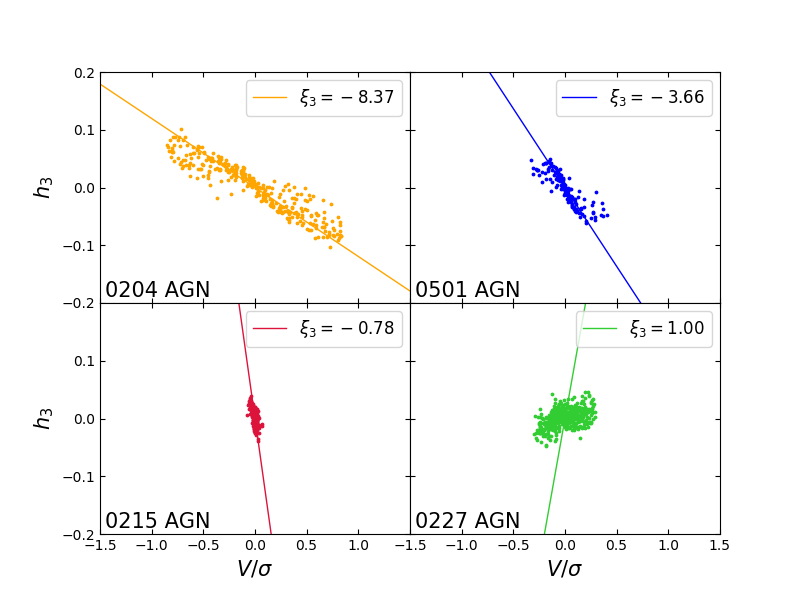
Figure 2: Four simulation examples for the relation between $h_{3}$ and $V_{\rm avg}$/$\sigma$ for the Voronoi bin within $R_{\rm e}$ with the corresponding $\xi_{3}$ values. The lines indicate $h_{3}=(1/\xi_{3})\cdot V_{\rm avg}/\sigma$. A typical axisymmetric fast rotator (0204 AGN) is shown in the upper left plot. It has the most negative $\xi_{3}$ value. The more complex fast rotator 0501 AGN(upper right panel) shows a steeper slope with a higher $\xi_{3}$. Slow rotators like 0215 AGN (bottom left panel) have $\xi_{3}$ close to zero. Unusual non-axisymmetric rotating systems like 0227 AGNhave a weak positive correlation between $h_{3}$ and $V_{\rm avg}$/ $\sigma$  resulting in a slightly positive value of $\xi_{3}$(bottom right panel).

3.2 Higher-order kinematics

The higher-order moments of the LOS velocity distribution, $h_{3}$ and $h_{4}$, can provide additional information on the orbital structure of our galaxies. In rotating systems the $h_{3}$ parameter has been observed to be anti-correlated to the average LOS velocity $V_{\rm avg}$, or more specifically to the $V_{\rm avg}$/$\sigma$ ratio (Gerhard, 1993; Krajnović et al., 2011; Veale et al., 2017; van de Sande et al., 2017). This anti-correlation indicates that the LOS velocity distributions typically have a steep leading wing and a broad trailing wing. Simple axisymmetric rotating stellar systems show this property due to projection effects - stars are typically on circular orbits and those with lower LOS velocities projected into each spaxel produce a broad trailing wing. The slope of this anti-correlation is then about $\sim 0.1$ (Bender et al., 1994). However, if the galaxy is more complex, i.e not axisymmetric, it can also contain stars orbiting around different axes or radial orbits. This can make the trailing wing broader, as these stars have lower LOS velocities. The slope of the anti-correlation would then be steeper, and in some slow-rotating galaxies it can become extremely steep (see e.g. van de Sande et al., 2017). If he group of rotating stars becomes sub-dominant the correlation between $h_{3}$ and $V_{\rm avg}$ / $\sigma$  can change sign and become positive. Here the few fast rotating stars create a broad leading wing in the LOS velocity distribution Naab et al. (2006); Hoffman et al. (2009); Röttgers et al. (2014). This unusual property is typically seen in simulated gas poor mergers Naab & Burkert (2001); Naab et al. (2014).

We characterise this variety of behaviours with a global parameter indicating the slope of the relation between $h_{3}$ and $V_{\rm avg}$ / $\sigma$ for all spaxels of one galaxy. This definition is inspired by the finding in Naab et al. (2014) that different slopes indicate varying formation histories and by the improved empirical classifications of the SAMI and MASSIVE galaxy surveys (van de Sande et al., 2017; Veale et al., 2017). We define $\xi_{3}$ as:

$$\xi_{3}=\frac{<h_{3}\cdot V_{\rm avg}/\sigma>}{<{h_{3}}^{2}>}=\frac{\sum_{i}F_{i}\,h_{3,i}\cdot(V_{i}/\sigma_{i})}{\sum_{i}F_{i}\,{h_{3,i}}^{2}},$$ (8)

where the sum is calculated over each spaxel out to $R_{\rm e}$ from the centre. When $h_{3}$ and $V_{\rm avg}$/$\sigma$ are correlated, this parameter estimates the inverse of the slope of the correlation to reasonable accuracy with a simple fraction of weighted sums; negative values indicate a negative correlation, while positive values indicate a positive one. This can be seen by assuming $<h_{3}>=0$ and $<V_{\rm avg}/\sigma>=0$ and rewriting the definition of the parameter as:

$$\xi_{3}=\rho_{V/\sigma,h_{3}}\,\frac{\sigma_{V/\sigma}}{\sigma_{h_{3}}},$$ (9)

where $\rho_{V/\sigma,h_{3}}$ is the Pearson (1895) correlation coefficient of $V_{\rm avg}$/$\sigma$ and $h_{3}$, and $\sigma_{V/\sigma}$ and $\sigma_{h_{3}}$ are the dispersion values of the two parameters. If $h_{3}$ and $V_{\rm avg}$/$\sigma$ are linearly correlated then $\rho=\pm-1$, and $\xi_{3}$ becomes exactly the slope of the correlation. Figure 2 shows an example of the $h_{3}$ - $V_{\rm avg}$ / $\sigma$ spaxel values within $R_{\rm e}$ for four simulated galaxies with different LOS velocity distribution properties. The lines indicate the simple slope given by $h_{3}=(1/\xi_{3})\cdot V_{\rm avg}/\sigma$. Purely rotating systems are expected to have $\xi_{3}\sim-10$ or lower, while rotating systems with non-negligible fractions of different orbit types are expected to lie in the $-3<\xi_{3}<-6$ range. When there is no correlation, or when the slope is almost vertical (both of which are observed in slow-rotating galaxies), the value of $\xi_{3}$ comes close to zero. Additionally, the dependence of $\xi_{3}$ on inclination seems to be weaker than other kinematic global parameters, making it potentially a good way of distinguishing different types of galaxies. In Section 5.2 we investigate inclination effects and show how this parameter correlates with other galaxy properties. van de Sande et al. (2017) have used best fitting elliptical Gaussians with a maximum log-likelihood approach to characterise the slope of the relation, which is slightly more complicated than our procedure. Veale et al. (2017) perform linear least square fits to calculate the slopes directly. Using the inverse of the slopes highlights the difference between slow rotators and the slow rotators get values around zero. The $h_{4}$ parameter is known to relate to orbit anisotropy (van der Marel & Franx, 1993; Gerhard, 1993; Thomas et al., 2007), with negative values indicating the dominance of tangential orbits and positive values corresponding to radial orbits. We do not further analyse $h_{4}$ other than showing the projected maps.

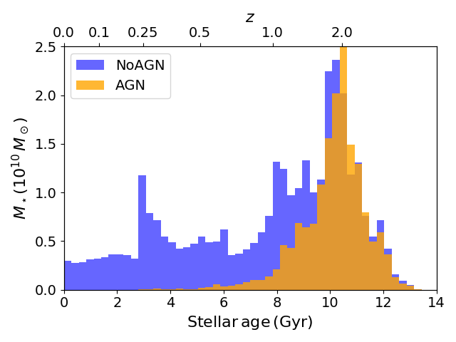
Figure 3: Age distribution of star particles in the case study galaxy (0227) for the run with AGN feedback (orange) and the one without (blue). The top x-axis shows the corresponding redshift at which the stars have formed. Star formation proceeded at a similar rate up $z=2$. Then it is rapidly terminated in the presence of AGN feedback. Without AGN feedback star formation continues all the way to $z=0$.

3.3 Isophotal shape and triaxiality

Our analysis involves the calculation of photometric quantities, such as the ellipticity $\epsilon$ and the isophotal shape parameter $a_{4}/a$. The ellipticity values are calculated by fitting the galaxy isophotes with ellipses. The isophotes are constructed as lines with constant stellar surface mass density. For each galaxy we use 10 isophotes between $0.25R_{\rm e}$ and $R_{\rm e}$ and average their ellipticity values to obtain $\epsilon$ . The $a_{4}/a$ parameter represents the deviation of the shape of the isophotes of the galaxy from a perfect ellipse. It is used to discriminate between galaxies with ‘boxy’ or ‘disky’ isophotes (Lauer, 1985; Bender & Moellenhoff, 1987). We calculate it by applying a Fourier expansion to the deviation of the actual isophotes from their best-fitting ellipse:

$$\delta\,R(\theta)=R(\theta)-R_{ell}(\theta)=\sum_{n}(a_{n}\,\cos(n\,\theta)+b_{n}\,\sin(n\,\theta)),$$ (10)

where $\theta$ is the azimuthal angle (Jedrzejewski, 1987). The first, second and third order coefficients are negligible if the ellipse is centred correctly and has the correct ellipticity and orientation angle. The fourth order coefficient $a_{4}$, normalised to the zeroth coefficient $a$, represents the deviation of the isophote from a pure ellipse. A positive value of $a_{4}/a$ means that there is an excess of light along the major axis of the ellipse, causing the real isophote to be more ‘disky’. A negative value instead means that the shape of the real isophote is more ‘boxy’ (see e.g. Naab et al., 1999; Springel, 2000).
We also look at the 3D shape of our galaxies by computing the triaxiality parameter:

$$T=\frac{1-(b/a)^{2}}{1-(c/a)^{2}},$$ (11)

where $b/a$ and $c/a$ are the ratios between the main axes. We calculated the axis ratios through the reduced inertia tensor (Bailin & Steinmetz, 2005) of all particles within the effective radius $R_{\rm e}$:

$$\tilde{I}_{i,j}=\sum_{{\rm Particles}\,k}m_{k}\frac{r_{k,i}\,r_{k,j}}{r_{k}^{2}},$$ (12)

where $m_{k}$ and $\vec{r}_{k}$ are the masses and positions of the particles. The square roots $\tilde{a}>\tilde{b}>\tilde{c}$ of the eigenvalues of this tensor are related to the real axis ratios by:

$$\tilde{b}/\tilde{a}=(b/a)^{\sqrt{3}}\;\;\;{\rm and}\;\;\;\tilde{c}/\tilde{a}=(c/a)^{\sqrt{3}}.$$ (13)

When $T=0$ the galaxy is perfectly oblate, while when $T=1$ the galaxy is perfectly prolate.

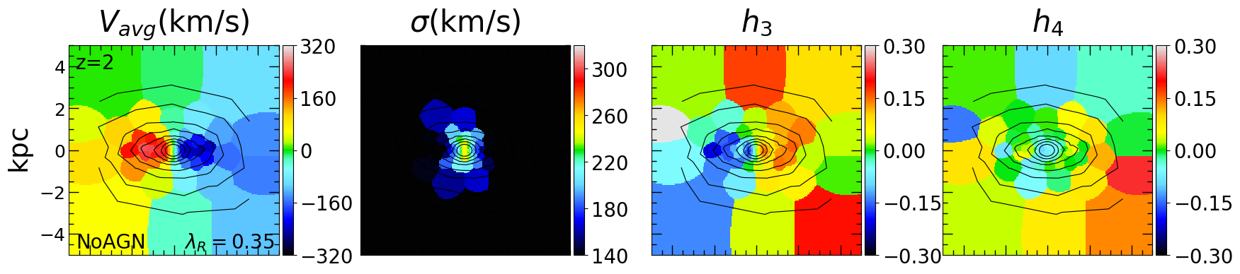
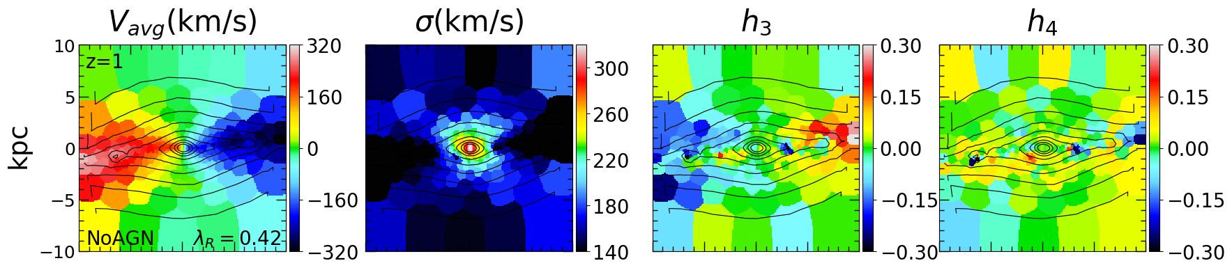
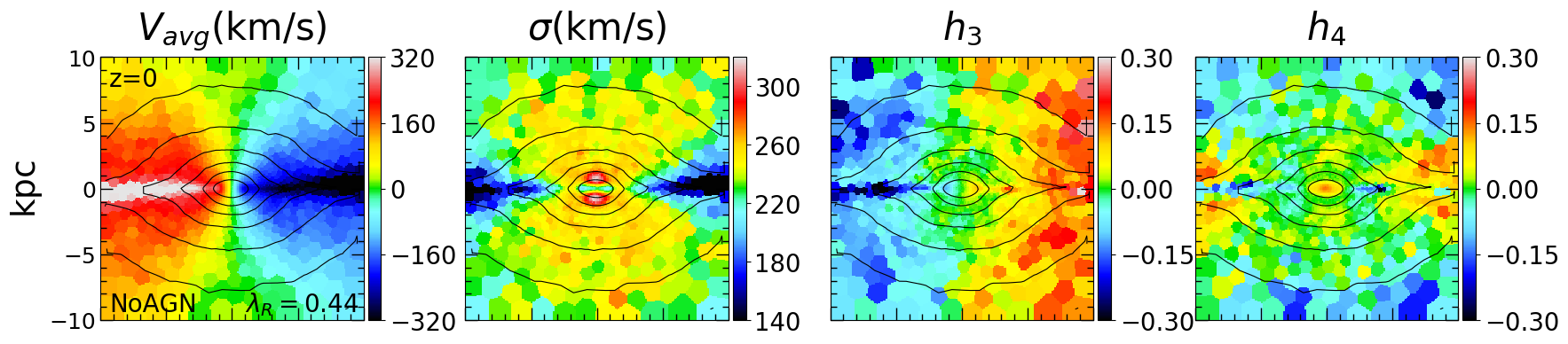
Figure 4: Edge-on two-dimensional line-of-sight stellar kinematics ($V_{\rm avg}$-$\sigma$-$h_{3}$-$h_{4}$  from left to right) of galaxy 0227 simulated without AGN feedback at $z=2$, $z=1$, and $z=0$ (from top to bottom). The maps shows typical features of systems with a disc-like component: high LOS velocity in the mid-plane, dumb-bell shaped velocity dispersion with a suppression in the mid plane disc region, anti-correlation of line-of-sight velocity and $h_{3}$  negative $h_{4}$ along the disc. These features become strongest at $z=0$, when the disc is most prominent and can clearly be seen in the surface density contours (black lines).

3.4 Orbit analysis

We analyse the orbital composition of each of our simulated galaxies following the approach of Jesseit et al. (2005) and Röttgers et al. (2014). This procedure starts by freezing the potential of the simulated galaxy at $z=0$ and representing it analytically using the self-consistent field method (Hernquist & Ostriker, 1992): the density and potential are expressed as a sum of bi-orthogonal basis functions, which satisfy the Poisson equation. There are multiple such density-potential pairs. We used the one from Hernquist & Ostriker (1992), in which the zeroeth-order element is the Hernquist (1990) profile:

$$\rho_{000}=\frac{M}{2\,\pi\,a^{3}}\frac{1}{\frac{r}{a}(1+\frac{r}{a})^{3}}$$ (14)

$$\Phi_{000}=-\frac{G\,M}{r+a},$$ (15)

where $a$ is the scale parameter of the Hernquist profile. Higher order terms then account for both radial and angular deviations. We then integrate the orbits of each stellar particle within this fixed analytical potential for about 50 orbital periods. This is enough for identifying the orbit type, but not so much that quasi-regular orbits diverge from regular phase-space regions forcing us to classify them as irregular. The orbit classification itself is then done using the code by Carpintero & Aguilar (1998), which distinguishes different orbit families by looking at the resonances between their frequencies along different axes. In this paper we consider 4 main families of orbits: z-tubes (orbits that rotate around the z axis), x-tubes (orbits that rotate around the x-axis), box orbits ($\pi$ boxes and boxlets), and irregular orbits. In addition to these, we computed the fraction of prograde z-tube orbits $f^{pro}_{z-tube}$, by only selecting z-tubes with angular momentum along the z-axis of the same sign as the overall galaxy.

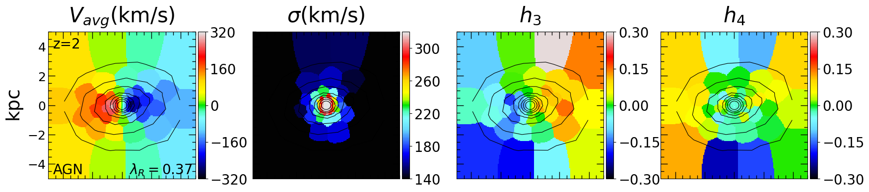
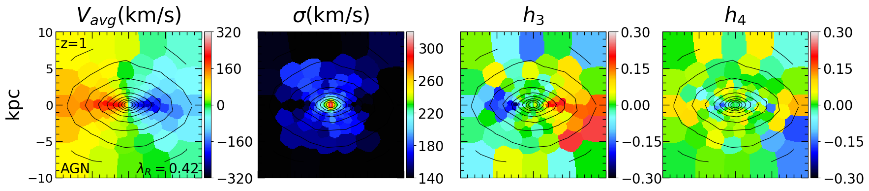
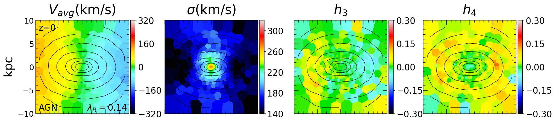
Figure 5: Same as Fig. 4 for galaxy 0227 simulated including AGN feedback. The kinematics is qualitatively similar to the case without AGN at $z=2$ and $z=1$. By $z=0$ however the strong rotational signatures are gone, and the galaxy looks more like a typical slow-rotator without kinematic disc signatures: low average LOS velocity, high velocity dispersion, no $h_{3}$ anti-correlation signal, positive $h_{4}$.

4 A typical galaxy simulated with and without AGN feedback

Our study involves a small sample of 20 massive galaxies. As a test case, in this section, we first discuss the formation history, global galaxy properties, stellar kinematics, stellar age and metallicity, morphology and redshift evolution for one prototypical galaxy. Simulating this initial condition with and without AGN feedback allows us to investigate the impact of AGN feedback on the final properties of the galaxy.

4.1 Formation history and global properties

Galaxy 0227 is an early-type galaxy, with an effective radius of $4.0\,{\rm kpc}$ and a stellar mass of $2\cdot 10^{11}\,M_{\odot}$ in the AGN case and $5\cdot 10^{11}\,M_{\odot}$ in the NoAGN case. Its formation history is characterised by a major merger at redshift $z\sim 0.25$, with mass ratio of $1:1.7$ and $1:1.2$ in the NoAGN and AGN cases. The presence of AGN has a strong influence on the evolution after the merger. Figure 1 shows a mock V-band image of this galaxy with and without AGN feedback. In the absence of AGN feedback (left panel) the galaxy is still forming new stars in an extended disc. Instead, in the case with AGN feedback (right panel) the system is spheroidal with a very old stellar population.

Figure 3 shows the age distribution of stars in galaxy 0227 simulated with and without AGN feedback. The oldest stars (age $>$ 10 Gyr) have very similar age distributions, with the bulk forming around $z\sim 2$. Towards lower redshifts, star formation gets quenched in the AGN case; a behaviour found in all our simulations. While in the AGN case not many stars form after $z\sim 1$, in the NoAGN case star formation continues throughout the simulation, including a starburst at $z\sim 0.25$ during the major merger.

4.2 LOS kinematics

In order to identify features in the stellar kinematics originating from the impact of AGN feedback, we construct two-dimensional maps visualising kinematic properties, as detailed in Sec. 3.1. Specifically we show the stellar line-of-sight velocity, dispersion, and the higher order moments $h_{3}$ and $h_{4}$ in Figs. 4 and 5 for galaxy 0227 without and with AGN feedback at $z=2$, $z=1$, and $z=0$. Initially (at $z=2$ and $z=1$) there are only moderate differences between the AGN and NoAGN simulations. The AGN and NoAGN galaxies (in brackets) have similar stellar masses of $M_{*}=0.59*10^{11}\,M_{\odot}$ ( $M_{*}=0.54*10^{11}\,M_{\odot}$ ) at $z=2$, while at $z=1$ they are $M_{*}\sim 1.16*10^{11}\,M_{\odot}$ ( $M_{*}\sim 1.97*10^{11}\,M_{\odot}$ ). The effective radii are $\sim 0.18\,\rm kpc$ ( $\sim 0.35\,\rm kpc$ ) at $z=2$ and $0.95\rm kpc$ ($1.53\rm kpc$) at $z=1$. Down to $z=1$, the galaxies are supported by rotation. The average stellar line-of-sight velocities reach values of $\sim 200\,{\rm km/s}$, and the velocity dispersion values around $300\,{\rm km/s}$. The velocity increases only slightly from $z=2$ to $z=1$, but the rotating component becomes more extended for both cases. The $h_{3}$ parameter is anti-correlated with the LOS velocity - a typical signature for axisymmetric rotating systems (Krajnović et al., 2011; Naab et al., 2014). The origin of this effect is explained in detail in Section 3.2, as well as in Naab & Burkert (2001); Naab et al. (2006); Röttgers et al. (2014); Naab et al. (2014) in the context of idealised models, merger simulations and cosmological simulations. At redshift $z=0$, the situation is markedly different. In the NoAGN case the rotation signatures are significantly enhanced. The LOS velocities reach up to $320\,{\rm km/s}$ in an extended disc. The velocity dispersion map shows a dumbbell feature with reduced velocity dispersion in the mid plane, which is a signature of an edge-on rotation-supported disc embedded in a dispersion-supported spheroidal component. This can be seen by the isophotes (see Sec. 4.4). The LOS velocity distribution is asymmetric with anti-correlated $h_{3}$ values. The $h_{4}$ map shows characteristic features of disc rotation (bottom right panel of Fig. 4). In the central kpc region, $h_{4}$ is positive, indicating a more peaked Gaussian LOS velocity distribution with more extended wings towards lower and higher than the systemic velocity as individual pixels cover significant fractions of the stars’ orbits. At larger radii (in the mid plane), $h_{4}$ becomes negative indicating coherent rotation with very weak tails towards high and low velocities. As $h_{4}$ is known to roughly correlate with the velocity anisotropy (Gerhard, 1993; Thomas et al., 2007), a negative $h_{4}$ indicates that tangentially biased orbits are dominating, which is to be expected in a rotating disc. Kinematic maps of this kind are regularly found in observational surveys like $ATLAS^{3D}$ (Cappellari et al., 2011b), CALIFA (Sánchez et al., 2012), or SAMI (Croom et al., 2012). They are, however, more common for less massive galaxies. It is very unlikely to observe an elliptical galaxy of this high mass with such a prominent fast-rotating disc. The kinematic galaxy properties are very different in the AGN case (Fig. 5). By $z=0$, there are no signatures of a prominent rotating stellar disc, as the AGN feedback prevents further gas accretion and in-situ disc formation (see e.g. Brennan et al., 2018). The galaxy is slowly rotating at $\sim 80\,{\rm km/s}$ and dispersion dominated, with only weak features in the higher-order moments. Interestingly, $h_{3}$ is positively correlated with $V_{\rm avg}$ in the central part of the galaxy. This is rare for observed galaxies, but relatively common in the simulated remnants of gas poor mergers (see Naab & Burkert, 2001; Naab et al., 2006; Röttgers et al., 2014). This positive correlation must originate from a particular orbital distribution, which will be analysed in Section 4.6. Also a core with negative $h_{4}$ is still visible. Values for $h_{4}$ are positive in most of the map indicating radially-biased orbits. All of the above features are typical properties of massive early-type galaxies.

4.3 Age and metallicity distribution at z=0

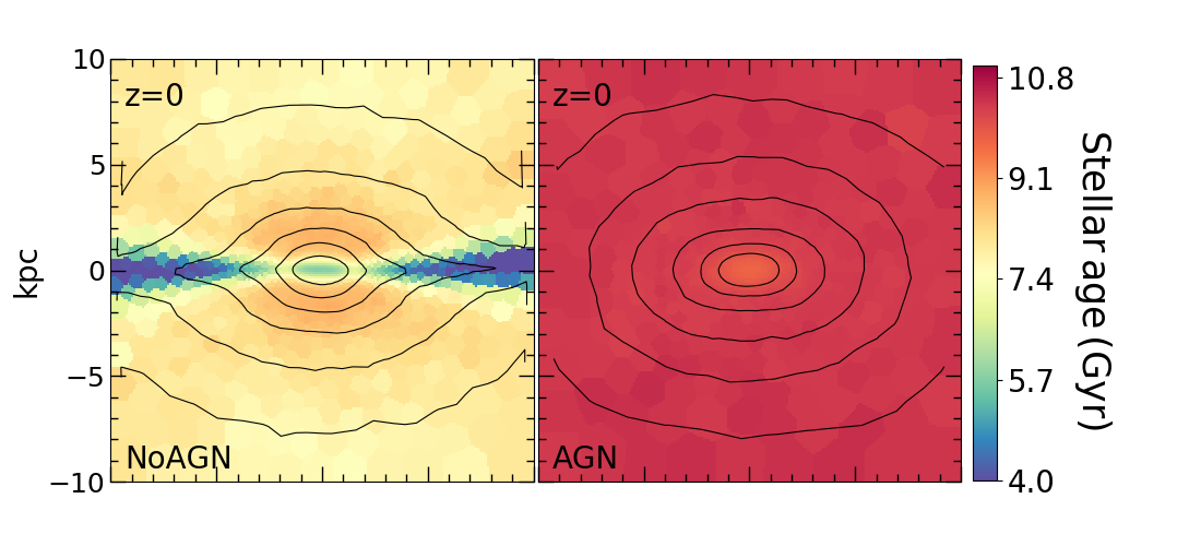
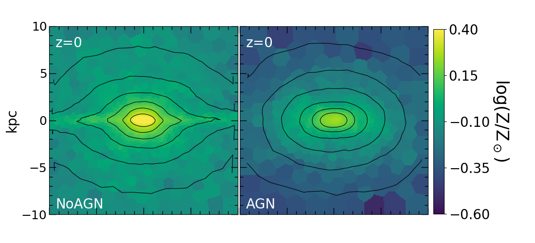
Figure 6: Voronoi binned maps of the (mass-weighted) average stellar age (top) and metallicity (bottom) for our case-study galaxy (0227), in the NoAGN (left) and AGN (right) AGN cases, at $z=0$. Without AGN feedback the higher star-formation rate at low redshift produces an overall much younger system, especially in the midplane, where a young stellar disc forms. Higher star-formation rate also result in high metallicities. With AGN feedback (right panels) the galaxy is instead very old and the metallicities compare well with observed early-type galaxies.

Figure 6 shows a comparison of the projected stellar age (top panels) and metallicity (bottom panels) distributions for the NoAGN (left column) and AGN (right column) simulation at $z=0$. At low redshifts the properties of the systems differ the most. In the NoAGN case there is a distinct young $\lesssim 4\,{\rm Gyr}$ stellar disc embedded in an older $7-9\,{\rm Gyr}$ stellar bulge. A moderate positive age gradient towards younger ages away from the centre is visible. The disc appears as a flattened metal enriched region in the mid plane, pretty much following the isophotes. These features indicate ongoing disc-like star formation and metal enrichment since $z=1$. This is also consistent with the stellar age distribution in Fig. 3. In the AGN case (right panels of Fig. 6) the stellar population is older ($\sim 10\,{\rm Gyr}$, see also Fig. 3), less metal enriched - due to less ongoing star formation - with a shallower metallicity gradient. There is a mild positive age gradient with younger ages in the centre caused by residual nuclear star formation. The origin of age and metallicity gradients will not be discussed further in this paper (see e.g. Hirschmann et al., 2015; Rodriguez-Gomez et al., 2016).

4.4 Redshift evolution of kinematic and photometric properties

In this subsection we look at the evolution of three global parameters, $\lambda_{R}$, $\xi_{3}$ and $a_{4}/a$, through the whole formation history of our case-study simulation. We first use $\lambda_{R}$ (Eq. 7) to quantify the redshift evolution of angular momentum in the AGN and NoAGN cases. Figure 7 shows the redshift evolution of $\lambda_{R}$ from $z=2$ to $z=0$. After a tumultuous phase at high redshift caused by mergers, at $z=1$ $\lambda_{R}$ settles at around $0.3$-$0.4$ in both cases. At $z=0.25$ the angular momentum drops because of the major merger described in Section 4.1; the vertical dashed line marks the beginning of this merger. The subsequent evolution diverges for the two cases. In the NoAGN simulation the system is more gas rich, and thus loses less angular momentum and even regains it after the merger. This is a typical feature of gas rich mergers and follow-up gas accretion (see review by Naab & Ostriker (2017)). In the AGN case the system is already gas poor, without significant star formation before the merger (see Fig. 3). The merger then reduces the angular momentum significantly. Qualitatively this process for gas poor mergers is discussed in detail in Naab et al. (2014). By $z=0$ the two systems have very different rotation properties with a $\lambda_{R}$ value typical of fast rotators in the NoAGN case and a slow rotator value in the AGN case. This impact of AGN feedback on the rotation properties of massive galaxies has already been reported by Dubois et al. (2013); Martizzi et al. (2014) and Dubois et al. (2016) for cosmological RAMSES adaptive mesh refinement simulations with different AGN feedback models. We therefore assume this to be a generic feature of AGN feedback.

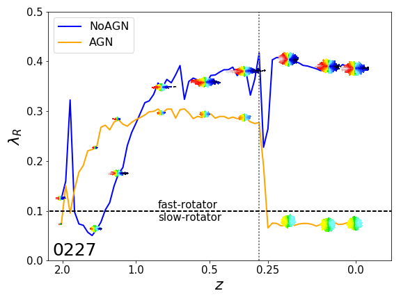
Figure 7: Evolution of $\lambda_{R}$ for galaxy 0227, in the NoAGN and AGN cases. The values are indicated by inserted velocity maps out to the effective radius (isophote) of the galaxies. A major merger at $z\sim 0.25$ (vertical dashed line) strongly reduces the angular momentum of both systems. The NoAGN galaxy is less affected and can quickly regain angular momentum due to gas accretion and star formation. The AGN galaxy is instead unable to form new stars and remains a slow rotator.

The major merger also affects the higher-order kinematic features. We quantify them using the parameter $\xi_{3}$ defined in Eq. 8 and plot it as a function of redshift, as shown in Figure 8. From $z=1$ to $z=0.25$ the two simulations show again the same behaviour, with the same degree of anti-correlation between $h_{3}$ and $V_{\rm avg}$ / $\sigma$: $\xi_{3}\sim-7.5$ in both cases. As discussed in section 3.2, this value is typical for a system dominated by tangential orbits, but higher than the one expected from a purely rotational system ($-10$). This indicates that a small amount of other orbit types contributes to skew the LOS velocity distribution. The major merger at $z=0.25$ again makes the two cases diverge. In the NoAGN case the overall $\xi_{3}$ value stays the same. In the AGN case instead $\xi_{3}$ drops to $0$ and the orbital structure of the system is more dispersion-supported - the correlation between $h_{3}$ and $V_{\rm avg}$/ $\sigma$ becomes weaker. The sign of $\xi_{3}$ oscillates a bit, but then settles to a weakly positive value, meaning that $h_{3}$ has the same sign as $V_{\rm avg}$ as already pointed out.

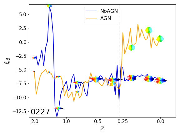
Figure 8: Evolution of $\xi_{3}$ for galaxy 0227, in the NoAGN and AGN cases. The values are indicated by small velocity maps out to the effective radius (isophote) of the galaxies. Up to $z=0.25$ the value of $\xi_{3}$ is constant for both simulations and has a value as expected for a rotating system. However, after a major merger at $z\sim 0.25$ (vertical dashed line), the value for the AGN galaxy shifts towards zero and mildly positive values. This indicates that the galaxy lost its rotational support.

We investigate the evolution of the isophotal shape parameter $a_{4}/a$, obtained by fitting the galactic isophotes at every snapshot (see subsection 3.3), with the galaxy seen edge-on. An example of these isophotes can be seen in the black lines of Figs. 4 and 5. We show the evolution of $a_{4}/a$ since $z=2$ in Fig. 9. Unlike in the previous cases, the AGN and NoAGN cases are already different at $z=1$. The NoAGN case has systematically higher values of $a_{4}/a$ - more disky isophotes. This difference would however not be as pronounced if the galaxy was not seen from an edge-on perspective. The value scatters due to minor mergers but drops to negative values after the major merger at $z=0.25$. This is the common feature of major mergers destroying previously existing disc structures (see Naab et al., 1999; Naab & Burkert, 2003). Subsequently a new stellar disc forms and the $a_{4}/a$ value becomes strongly positive again. In the AGN case the galaxy already lost its diskyness at high redshift, because of the suppressed inflow of high-angular-momentum star-forming gas, and it keeps its elliptical or mildly boxy isophotes to $z=0$. The effect of mergers and AGN feedback on the isophotal shape points in the same direction as the effect on $\lambda_{R}$ and $\xi_{3}$.

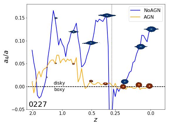
Figure 9: Evolution of the isophotal shape of galaxy 0227, in the AGN and NoAGN case, quantified by $a_{4}/a$. The markers are surface brightness maps cut along the effective isophote. The red line represents perfectly elliptical isophotes. ‘Boxy’ galaxies have negative, ‘disky’ galaxies have positive $a_{4}/a$ values. Without AGN feedback the formation of a prominent disc results in disky isophotes at all times, despite the major merger at $z\sim 0.25$ (vertical dashed line). The AGN galaxy instead loses its diskyness after the merger because further star formation is suppressed by the AGN.

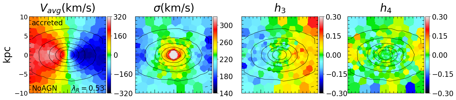
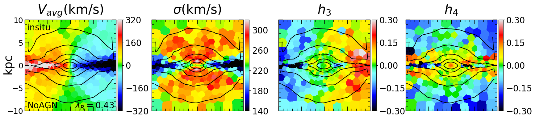
Figure 10: Stellar kinematics of galaxy 0227 (NoAGN) separated into its accreted component (above) and its in-situ formed one (below). The overall in-situ fraction is 50% . The two components have strikingly different kinematics. The accreted component is mainly pressure-supported, but also rotates fast. The in-situ component shows two distinct features: a fast-rotating disc in the midplane with low velocity dispersion, and a slow-rotating bulge with very high velocity dispersion. The disc feature formed after a recent major merger, while the surrounding bulge is older, and its originally rotational orbits have been scrambled by the merger.

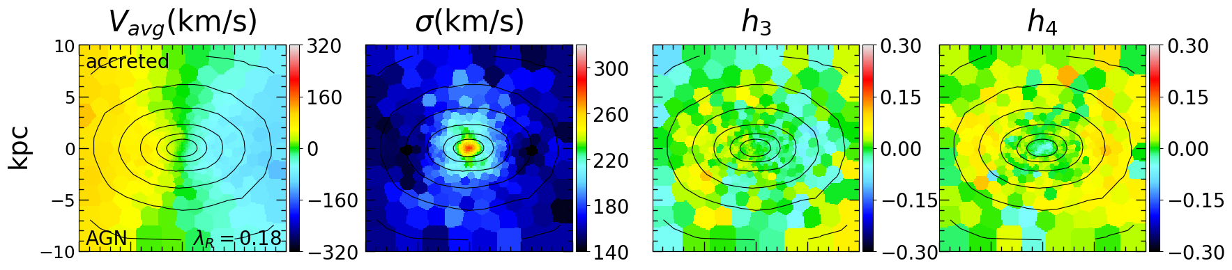
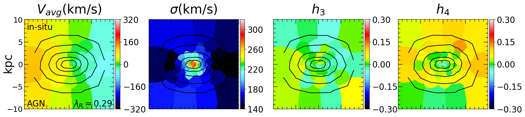
Figure 11: Stellar kinematics of the accreted (above) and in-situ formed (below) stars of galaxy 0227 simulated with AGN feedback. The overall in-situ fraction is 17% . In both cases the kinematics are pressure-supported, as no star formation happened since the last major merger at $z=0.25$.

4.5 Kinematics of the accreted and in-situ-formed stellar components

Our kinematic maps can be generated for different stellar components of the galaxy, to shed light on their respective kinematic structure. One might use the stellar age to distinguish different components; we show this example in the appendix. Perhaps even more interesting though, is to separate stellar particles according to their origin: either accreted from another galaxy or formed in-situ in the main progenitor following the accretion of gas. Due to their intrinsically different origin, we can expect these two components to show very different kinematic (and stellar population) signatures (see e.g. Naab et al., 2014). To classify stars as in-situ or accreted, we trace stars in the galaxies throughout the simulation from $z=2$ to $z=0$, and label them as in-situ stars when they form within ten per cent of the virial radius (see Oser et al., 2010). All the remaining stellar particles are labelled as accreted. In the case of galaxy 0227 the in-situ fraction is $f_{\rm in-situ}=0.50$ and $f_{\rm in-situ}=0.17$ for the NoAGN and AGN cases, respectively. The values for the other galaxies are shown in Table 1.
Figures 10 and 11 show the stellar kinematic maps obtained for the separated in-situ and accreted components, in the NoAGN and AGN cases respectively. The accreted components (upper panels of Fig. 10 and 11) exhibit a very high velocity dispersion in both cases, but also have considerable net rotation, especially in the NoAGN case. This larger net rotation is probably caused by the potential being more oblate-shaped in the NoAGN simulation ($T=0.41$). In the AGN case the galaxy has a very triaxial, almost prolate shape ($T=0.86$), which hinders the amount of z-tube orbits (more on this in Section 4.6) causing less rotation.
The in-situ components are very different in the two cases. In the AGN case (lower panel of Fig. 11), the in-situ stars follow the same kinematics as the accreted ones. Almost all of these stars formed before the major merger at $z=0.25$, which means that their original orbits have been scrambled, resulting in a dispersion-supported system. In the NoAGN case the number of in-situ-formed stars is larger, both before and after the major merger, and the corresponding kinematic maps are more complex. There are two distinct features. The first is an orderly fast-rotating disc in the midplane, with low velocity dispersion, a shallow $h_{3}$$V_{\rm avg}$/$\sigma$trend, and strongly negative $h_{4}$. The second is a slow-rotating bulge with high velocity dispersion and a much steeper trend with $h_{3}$. The first component is mostly made of young stars which formed after the $z=0.25$ major merger, hence the orderly motion. The surrounding bulge is instead older. These stars formed in-situ at $z>0.25$, and their orbits have been scrambled because of the major merger, resulting in less rotation. As the very high velocity dispersion suggests, there is also a counter-rotating component in this bulge, which explains why this component has a smaller net rotation than the accreted stars in the same potential.
This analysis implies that in-situ-formed stars and accreted stars tend to have intrinsically different kinematics from one another, at least until a major merger happens and scrambles their orbits. AGN feedback can thus significantly alter the present-day kinematics of galaxies by ‘freezing’ the kinematics at the most recent major merger, affecting the orbits of both accreted and in-situ-formed stars.

4.6 Orbit distribution

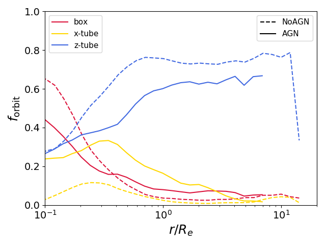
Figure 12: Radial frequency of three different types of orbits in our case study galaxy: z-tubes, x-tubes and boxes. The dashed line shows the NoAGN case, and the full line shows the AGN one. In the latter, the fraction of z-tube orbits drops considerably due to the suppression of disc formation, and the fraction of x-tube orbits increases due to the more triaxial potential.

It is also of interest to directly study the distribution of stellar orbits, and how it is affected by AGN feedback. We classify star particles into three global orbit types: z-tubes (rotating around the z-axis), x-tubes (rotating around the x-axis, including inner and outer major axis tubes) and boxes (including $\pi$-boxes and boxlets). Figure 12 shows the fraction of these orbit families as a function of radius. In the NoAGN case, the fraction z-tube orbits is larger at almost all radii. This is expected given the very prominent disc that has formed at low redshift. The central region is nevertheless dominated by box orbits, and x-tubes are very rare. In the AGN case there are significantly less z-tube orbits at all radii; the overall drop is from 65% to 49%, and the central regions are the ones that were impacted the most. The fraction of box orbits is slightly lower in the centre and higher in the outskirts. What really changed is the fraction of x-tube orbits, which went from an overall 5% to 17%. The likely reason for this is that the potential of the AGN galaxy has a more prolate shape ($T=0.86$, instead of $T=0.41$ for the NoAGN case), allowing for this kind of orbits. This change in the balance of different orbit families also explains the positive correlation between $h_{3}$ and $V_{\rm avg}$/$\sigma$; the bulk of the LOS velocity distribution is made of x-tube, box and retrograde z-tube orbits, and the prograde z-tube orbits add a high-velocity tail to it.

5 Results from the simulation sample

So far we focused on a single, example galaxy. In this section we show more general results for all twenty galaxies in our sample. This analysis cannot reveal the statistical kinematic properties of quiescent galaxy populations from recent cosmological simulations (Dubois et al., 2016; Penoyre et al., 2017b; Lagos et al., 2017; Schulze et al., 2018). Instead, we would like to highlight the detailed impact of AGN feedback on massive galaxies for a few individual systems simulated at higher resolution. Table 1 shows for each galaxy in our sample the stellar mass $M_{\star}$  effective radius $R_{\rm e}$  the average stellar age, the in-situ formed fraction, the ellipticity $\epsilon$  the isophotal shape $a_{4}/a$ , the triaxiality parameter $T$, $\lambda_{R}$ , $\xi_{3}$ and the fraction of z-tube orbits $f_{\rm z-tube}$ . In general all our galaxies have a lower stellar mass with AGN feedback due to the quenching of star formation, while the effective radius increases due to less dissipation (e.g. Crain et al., 2015; Choi et al., 2018). In the following sections we will look at the distribution of kinematic ($\lambda_{R}$ , $\xi_{3}$ , orbit families) and morphological ($a_{4}/a$ , triaxiality) properties at $z=1$ and $z=0$, and how AGN feedback affects them.

GalID		$M_{\star}(10^{10}M_{\odot})$	$R_{e}$	avg. age (Gyr)	$f_{in-situ}$	$\epsilon$	$a_{4}/a$	$T$	$\lambda_{R}$	$\xi_{3}$	$f^{\rm pro}_{\rm z-tube}\$
0175	NoAGN	$26.73$	$1.86$	$7.85$	$0.23$	$0.24$	$0.017$	$0.72$	$0.08$	$-0.05$	$0.56$
0175	AGN	$18.93$	$2.57$	$10.72$	$0.10$	$0.35$	$0.001$	$0.51$	$0.12$	$-6.58$	$0.45$
0204	NoAGN	$19.59$	$3.09$	$8.17$	$0.65$	$0.78$	$0.196$	$0.29$	$0.46$	$-7.07$	$0.14$
0204	AGN	$16.41$	$2.06$	$9.50$	$0.31$	$0.37$	$0.026$	$0.15$	$0.36$	$-8.19$	$0.38$
0215	NoAGN	$27.79$	$1.76$	$9.61$	$0.28$	$0.38$	$0.042$	$0.48$	$0.37$	$-5.14$	$0.39$
0215	AGN	$7.38$	$1.70$	$11.26$	$0.12$	$0.31$	$0.018$	$0.50$	$0.02$	$-0.79$	$0.15$
0227	NoAGN	$48.46$	$3.27$	$7.72$	$0.50$	$0.49$	$0.124$	$0.41$	$0.47$	$-8.10$	$0.27$
0227	AGN	$22.24$	$2.60$	$9.95$	$0.17$	$0.15$	$0.000$	$0.86$	$0.10$	$0.50$	$0.62$
0290	NoAGN	$26.32$	$2.95$	$8.55$	$0.56$	$0.71$	$0.112$	$0.28$	$0.52$	$-11.49$	$0.48$
0290	AGN	$12.67$	$2.57$	$10.45$	$0.29$	$0.38$	$0.045$	$0.66$	$0.06$	$-2.62$	$0.38$
0408	NoAGN	$7.57$	$1.88$	$9.12$	$0.32$	$0.24$	$0.020$	$0.68$	$0.07$	$1.82$	$0.68$
0408	AGN	$15.98$	$2.59$	$8.84$	$0.58$	$0.43$	$0.055$	$0.32$	$0.36$	$-6.41$	$0.27$
0501	NoAGN	$6.80$	$1.74$	$10.71$	$0.14$	$0.33$	$0.029$	$0.22$	$0.42$	$-6.74$	$0.59$
0501	AGN	$8.25$	$1.93$	$11.22$	$0.16$	$0.30$	$0.018$	$0.44$	$0.10$	$-3.55$	$0.62$
0616	NoAGN	$8.61$	$1.29$	$8.87$	$0.30$	$0.38$	$0.055$	$0.09$	$0.04$	$-1.02$	$0.17$
0616	AGN	$4.56$	$1.53$	$11.07$	$0.09$	$0.35$	$0.010$	$0.36$	$0.35$	$-7.27$	$0.08$
0664	NoAGN	$8.04$	$1.15$	$9.50$	$0.35$	$0.41$	$0.031$	$0.37$	$0.44$	$-5.74$	$0.69$
0664	AGN	$7.23$	$1.38$	$10.51$	$0.22$	$0.43$	$0.052$	$0.09$	$0.32$	$-7.61$	$0.56$
0858	NoAGN	$3.67$	$2.25$	$8.97$	$-1.00$	$0.36$	$0.045$	$0.25$	$0.49$	$-6.02$	$0.49$
0858	AGN	$6.99$	$1.93$	$8.11$	$0.49$	$0.26$	$0.006$	$0.38$	$0.31$	$-7.20$	$0.37$

Table 1: General properties of our sample of simulated galaxies.

5.1 Angular momentum

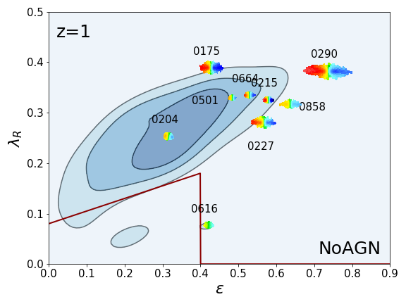
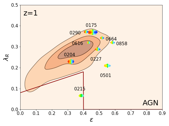
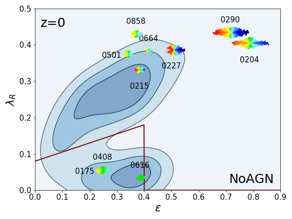
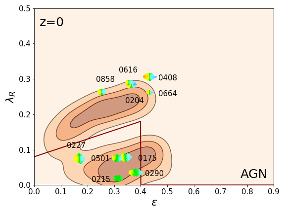
Figure 13: $\lambda_{R}$ as a function of ellipticity $\epsilon$ for the galaxies at redshift $z=1$ (top panels) and $z=0$ (bottom panels), simulated without (NoAGN, left) and with (AGN, right) AGN feedback. The edge-on values are indicated by velocity maps. The coloured contours indicate the distribution of our galaxies when they are seen from 50 random orientations each. The dark red line marks the limit between slow- and fast-rotators according to Cappellari (2016). With AGN feedback the systems become rounder and rotate more slowly at z=0.

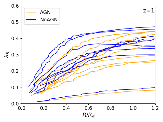
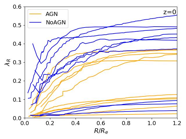
Figure 14: $\lambda_{R}$ radial profiles of our galaxy sample at z=1 (top) and z=0 (bottom). The AGN galaxies (orange) evolve towards lower $\lambda_{R}$ values than their NoAGN counterparts (blue).

In Fig. 13 we plot the $\lambda_{R}$ parameter of the sample galaxies versus their ellipticity $\epsilon$ for the simulations without (NoAGN, left panels) and with AGN (AGN, right panels) at redshift $z=1$ (top panels) and $z=0$ (bottom panels). The location of edge-on projections are indicated by the velocity maps. The blue/orange shaded regions indicate the typical distribution of these systems for random orientations (projection effects for $\lambda_{R}$ based on simulations are discussed in e.g. Jesseit et al., 2009; Naab et al., 2014; Lagos et al., 2018). They were obtained by calculating $\lambda_{R}$ and $\epsilon$ for 50 random lines-of-sight for each galaxy. The red line separates slow- and fast-rotators following to the definition by Cappellari (2016). A galaxy is considered a slow-rotator when

$$\lambda_{R}<0.08+0.25\,\epsilon{\hskip 14.22636pt\rm with\hskip 14.22636pt}\epsilon<0.4.$$ (16)

The distribution of galaxies at $z=1$ is similar between the AGN and NoAGN cases, with most galaxies being flattened fast-rotators with $\lambda_{R}$ in the range $0.2<\lambda_{R}<0.4$. The ellipticity values are a bit higher in the NoAGN case ($0.3<\epsilon<0.8$) than in the AGN one ($0.3<\epsilon<0.6$), but qualitatively the two populations are very similar. By $z=0$ many (7 out of 10) of the NoAGN galaxies are still fast rotators with a similar ellipticity distribution. This trend is in agreement with results for massive galaxy populations from cosmological box simulations without AGN feedback Dubois et al. (2016). Instead, in the AGN case by $z=0$ the galaxies have become rounder ($\epsilon<0.4$) and more slowly rotating, with $\lambda_{R}$ no larger than $\sim 0.35$. More than half of the galaxies would be considered bona-fide slow rotators even in their edge-on projections. As discussed earlier, the trend towards slower rotation with AGN feedback is caused by the suppression of late in-situ star formation (see Brennan et al., 2018 for a discussion of ejective and preventative AGN feedback), which in most cases significantly reduces rotation observed at $z=0$. The effect is strongest for the largest and most massive galaxies in our samples (lower numbers, like 0227), which - without AGN feedback - develop massive fast-rotating disc structures (In the case of galaxy 0175, this young disc structure is on a different plane, and thus does not increase $\lambda_{R}$ significantly).

We find a correlation between $\lambda_{R}$ and $\epsilon$, at least for the fast-rotators: faster rotating galaxies tend to be more flattened. Most of our slow-rotating galaxies exhibit a relatively high ellipticity, which is a trend found in other simulation studies as well(Bois et al., 2010; Naab et al., 2014), and possibly due to resolution limits. An interesting case is galaxy 0616, which contradicts our expectations by being a slow-rotator when simulated without AGN feedback but turns into a fast-rotator when simulated with AGN feedback. What happens here? In the NoAGN case gas infall triggers a starburst that forms a disc that counter-rotates with respect to the rest of the galaxy. This lowers the projected $\lambda_{R}$ value, but leaves a relatively high ellipticity. In the AGN case the gas is kept from forming this new disc and the galaxy retains most of the (projected) angular momentum of the older stellar component.
In Figure 14 we plot the $\lambda_{R}$ radial profiles for all galaxies, at $z=1$ and $z=0$. Typically, the values increase from the centre until they reach an asymptotic value, usually within $R_{e}$. This is consistent with previously published simulation data, even though we are missing systems with dropping $\lambda_{R}$ profiles (Naab et al., 2014; Wu et al., 2014; Lagos et al., 2018). At $z=1$ there is not much difference between the AGN and NoAGN galaxies, while at $z=0$ galaxies simulated with AGN feedback show once again systematically lower $\lambda_{R}$ values, even among the fast-rotators. Many galaxies that would be rotationally-supported without AGN, become pressure-supported when an AGN is present. Overall, AGN feedback results in more slow-rotating and dispersion-supported galaxies in agreement with previous simulations (Dubois et al., 2016) and the statistics of observed early-type galaxies.

5.2 Higher-order kinematics and orbital structure

As discussed in sections 3.2 and 4.4, rotating galaxies are expected to have anti-correlated $h_{3}$ and velocity fields, but the degree of this anti-correlation depends on the orbital structure of the galaxy, and we can employ our $\xi_{3}$ parameter to evaluate this for our sample. In Figure 15 we plot $\xi_{3}$ as a function of $\lambda_{R}$ at $z=1$ and $z=0$. The edge-on values are plotted with velocity maps, while the contours represent the location of the sample in the $\xi_{3}$- $\lambda_{R}$ plane for random orientations. Generally, the edge-on $\xi_{3}$ values are larger in absolute value, but for different inclinations the dependence of $\xi_{3}$ on the viewing angle is weak. At $z=1$ all galaxies have a negative of $\xi_{3}$ and $h_{3}$ is anti-correlated with the velocity, as expected for fast-rotators. This is also true for the two galaxies which are slow-rotators (according to $\lambda_{R}$) at $z=1$. At $z=0$ the sample splits into two groups: slow-rotators with low values of $\lambda_{R}$ tend to have $\xi_{3}\sim 0$ (very steep correlation or no correlation), while all fast-rotators have $\xi_{3}\ <-3$ (negative correlation). The specific value of $\xi_{3}$ for the fast-rotators depend on their orbital structure; the galaxies where a disc feature is particularly prominent (0204, 0227 and 0290 in the NoAGN case) have the lowest values, reaching about $\xi_{3}=-11.5$. In other words, more flattened and simple rotating systems have a less steep correlation between $h_{3}$ and $V_{\rm avg}$/$\sigma$ than fast-rotators with more complex kinematics. A similar behaviour was also observed in real galaxies by Veale et al. (2017). This results in a weak correlation between $\xi_{3}$ and $\lambda_{R}$ for the fast-rotators, that was not present at $z=1$ when the kinematics of the galaxies were overall simpler. The bi-modality of slow- and fast-rotators in the $\xi_{3}$-$\lambda_{R}$ plane is seen in both the NoAGN and AGN cases, but with AGN feedback the group of galaxies with $\xi_{3}\sim 0$ is larger. A few galaxies have a positive value of $\xi_{3}$ at $z=0$. One of them, 0227 AGN, has already been extensively discussed. The other one, 0408 NoAGN, has a positive value because of a sub-dominant rotating component in an otherwise dispersion-supported system, producing a positive correlation between $h_{3}$ and $V_{\rm avg}$.
If we compare these results with observational IFU surveys, we find a small discrepancy. In Figure 16 we plot the $\xi_{3}$ values of galaxies from the ${\rm ATLAS}^{3D}$ survey (Cappellari et al., 2011b), compared with the contours of our AGN simulations seen at random inclinations. The ${\rm ATLAS}^{3D}$ values also include a re-extraction of the kinematics from the subset of galaxies in the SAURON survey originally presented in Emsellem et al. (2004). To compute $\xi_{3}$ and $\lambda_{R}$ for the ${\rm ATLAS}^{3D}$ sample, we only considered spaxels with $\sigma>120\rm km/s$, since the Gauss-Hermite moments can only be extracted from the data when the galaxy velocity dispersion is well resolved by the spectrograph (e.g. Cappellari & Emsellem, 2004). The distribution of $\xi_{3}$ values is similar between observations and simulations, and can be divided in two groups: slow-rotators with $\xi_{3}\sim 0$ and fast-rotators with $-3<\xi_{3}<-10$. However, at given $\lambda_{R}$the ${\rm ATLAS}^{3D}$ galaxies seem to have lower $\xi_{3}$(in absolute value) than the simulations. We believe there are at least three reasons for this difference. Several of the ${\rm ATLAS}^{3D}$ fast-rotators have strong bar features, which are not present in our sample of simulations. In their presence the kinematic maps often show a positive correlation between $V_{\rm avg}$ and $h_{3}$ (Chung & Bureau, 2004), causing $\xi_{3}$ values closer to zero or sometimes even positive. In Figure 16 galaxies with clear bars have been highlighted, but hidden or weak bars could be present in the other galaxies too, affecting the $h_{3}$ values. Secondly, as previously mentioned, constraining the $h_{3}$ value of each spaxel is harder in observations. The selection of spaxels with $\sigma>120\rm km/s$ limits this problem, but does not eliminate it. This results in more noisy $h_{3}$ maps, which makes the $h_{3}$-$V_{\rm avg}$/$\sigma$ trend less tight, and thus moves the $\xi_{3}$ value of observed galaxies closer to zero. At equal $\sigma$, this effect is stronger for slower-rotating galaxies, as their LOS velocity distribution have lower $h_{3}$ values. Lastly, our (AGN) sample consists of only 10 massive galaxies, all of which have relatively low $\lambda_{R}$values. This means that our simulations do not explore the $\lambda_{R}>0.3$ regime, but if they did, we would expect most of them to have $-10<\xi_{3}<-5$, like many of the galaxies in our NoAGN sample, matching the observations.

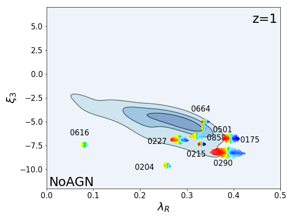
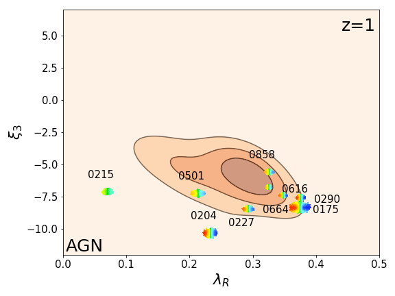
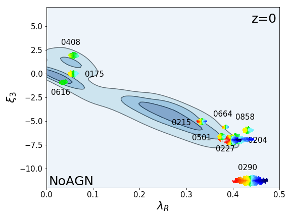
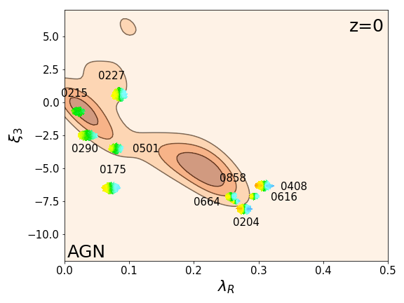
Figure 15: $\xi_{3}$ versus $\lambda_{R}$ at $z=1$ (top panels) and $z=0$ (bottom panels), simulated without (left) and with (right) AGN feedback. The kinematic map markers indicate the values when the galaxy is seen edge-on, while the density contours indicate the distribution when our galaxies are seen through 50 random orientations each. At $z=1$ all galaxies have have values of $\xi_{3}$ in the anti-correlation regime, typical of fast-rotators, while at $z=0$ many galaxies have $\xi_{3}\ \sim 0$ or in a few cases even positive, and this effect is stronger with AGN feedback.

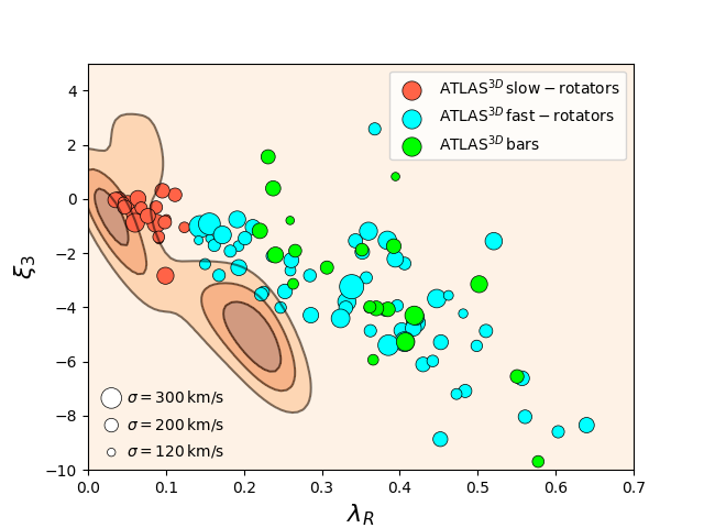
Figure 16: $\xi_{3}$ as a function of $\lambda_{R}$ for the galaxies from the ${\rm ATLAS}^{3D}$ sample (circle markers), compared with our AGN simulations (orange contours; same as Figure 15). The ${\rm ATLAS}^{3D}$ galaxies are distinguished in slow-rotators (red) and fast-rotators (light blue) according to the Cappellari (2016) definition. At equal $\lambda_{R}$, observed fast-rotators seem to have smaller $\xi_{3}$ (absolute) values than the simulation, possibly because of more complex kinematic features (bars) and of more noisy $h_{3}$ measurements. Slow-rotators have $\lambda_{R}\sim 0$ and $\xi_{3}\sim 0$ in both observations and simulations.

5.3 Orbit distribution and $\xi_{3}$

We would also like to see how closely connected $\xi_{3}$ is to the actual orbital structure of galaxies, measured in the same way as in Sections 3.4 and 4.6. In Figure 17 we plot $\xi_{3}$ as a function of the fraction of prograde z-tube orbits within $R_{\rm e}$, $f^{\rm pro}_{\rm z-tube}$, at $z=0$. The plotted $\xi_{3}$ values are the average for 50 random views of each galaxy, and the error bars mark the dispersion (negligible for galaxies 0616 NoAGN and 0215 AGN). Most galaxies with high values of $f^{\rm pro}_{\rm z-tube}$ have a $\xi_{3}<-3$ as expected, and there is a rough correlation between the two quantities. The galaxy with the highest $f^{\rm pro}_{\rm z-tube}$ (0290 NoAGN) is also the one with the lowest value of $\xi_{3}$: $\sim-11.5$ when seen edge-on and $\sim-6.5$ when averaging between many different viewing angles. The reason for this is that when the system is dominated by orbits that rotate (progradely) around the z axis, these stars form the bulk of the LOS velocity distribution, and all other orbit types make the $h_{3}$ signal stronger for that given $V_{\rm avg}$/$\sigma$. When non-rotational orbits are dominating ($f^{\rm pro}_{\rm z-tube}\ \sim 0$), then $V_{\rm avg}/\sigma\sim 0$ and consequently $\xi_{3}\ \sim 0$.
A few galaxies (0175 NoAGN, 0408 NoAGN and 0227 AGN) have a positive correlation between $h_{3}$ and $V_{\rm avg}$/$\sigma$ in large parts of their kinematic maps, resulting in a positive value of $\xi_{3}$. This is likely connected to the fact that these galaxies have a prolate potential. We investigate this by plotting $\xi_{3}$ as a function of the triaxiality parameter $T$ in Figure 18. There seems to be a rough correlation between the two quantities in our sample. The most prolate galaxies ($T\sim 1$) have positive values of $\xi_{3}$, while almost all oblate galaxies ($T<<1$) have negative values. The one exception is galaxy 0616 NoAGN, which as already discussed is made of two counter-rotating components and looks like a ‘fake’ slow-rotator.
This connection between morphology and kinematics likely arises because different potential shapes allow different kinds of orbits; specifically, x-tubes are more common in prolate potentials. We see this by plotting $\xi_{3}$ as a function of the fraction of x-tube orbits $f_{x-tube}$ in Figure 19. There is again a rough correlation, meaning that galaxies with higher $f_{x-tube}$ are more likely to display a positive correlation between $h_{3}$ and $V_{\rm avg}$/$\sigma$ in their kinematic maps. This follows from the correlation between $f_{x-tube}$ and the triaxiality $T$, which has previously been observed in isolated (Jesseit et al., 2005) and cosmological simulations (Röttgers et al., 2014). It should however be noted that in a pure prolate system only x-tube orbits and box orbits are allowed, and if there is net rotation around the long axis $h_{3}$ and $V_{\rm avg}$/$\sigma$ become anti-correlated again. We do not see this in our sample because none of our galaxies is dominated by x-tube orbits (at most $f_{x-tube}=0.25$, for 0227 AGN).

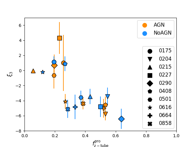
Figure 17: $\xi_{3}$ as a function of the fraction of prograde z-tube orbits $f^{\rm pro}_{\rm z-tube}$ for our sample of simulated galaxies at $z=0$. The $\xi_{3}$ values of each galaxy are an average over 50 random views, and the error bars are their standard deviation. Galaxies with high $f^{\rm pro}_{\rm z-tube}$ tend to have $\xi_{3}<-5$.

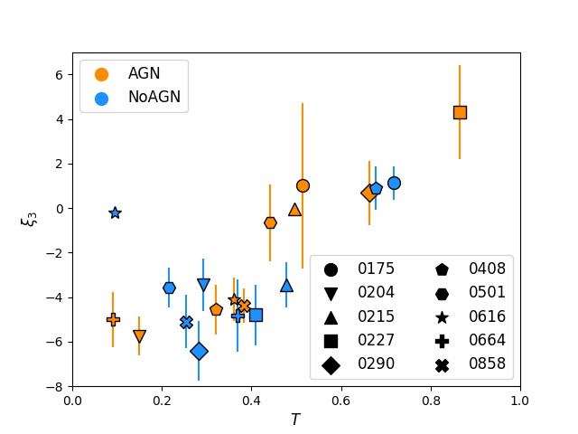
Figure 18: $\xi_{3}$ as a function of the triaxiality parameter for our sample of simulated galaxies at $z=0$. The $\xi_{3}$ values of each galaxy are an average over 50 random views, and the error bars are their standard deviation. There is a weak correlation between the two parameters: prolate galaxies have positive values of $\xi_{3}$ , while oblate galaxies have negative values.

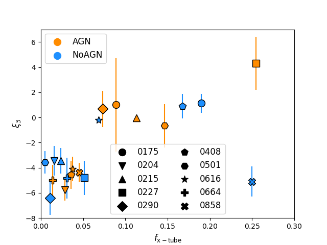
Figure 19: $\xi_{3}$ as a function of the fraction of x-tube orbits $f_{x-tube}$ for our sample of simulated galaxies at $z=0$. The $\xi_{3}$ values of each galaxy are an average over 50 random views, and the error bars are their standard deviation. Galaxies with high $f_{x-tube}$ tend to have $\xi_{3}>0$.

5.4 Isophotal shape

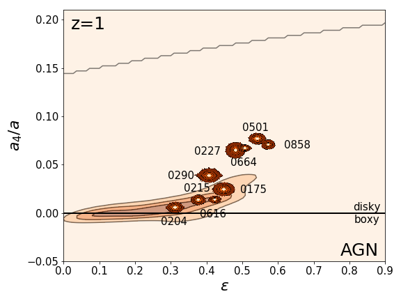
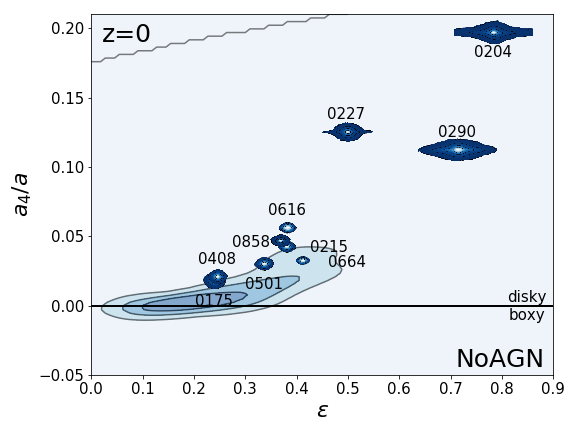
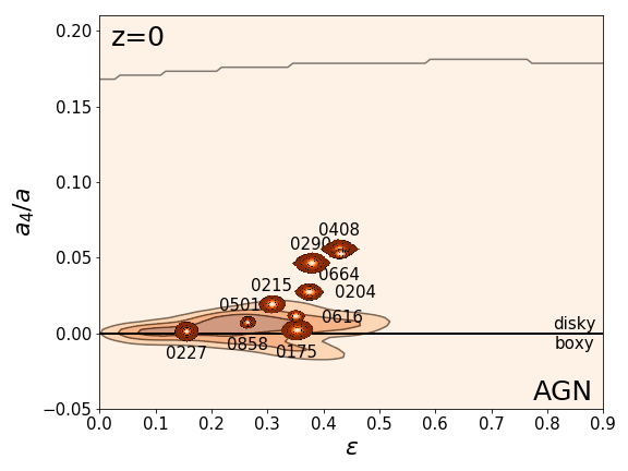
Figure 20: $a_{4}/a$ versus galaxy ellipticity $\epsilon$ at $z=1$ (top panels) and $z=0$ (bottom panels), simulated without (left) and with (right) AGN feedback. The edge-on locations are indicated by the isophotal maps, while the density contours indicate the distribution of our galaxies when they are seen from 50 random orientations each. The black line indicates elliptical isophotes and separates boxy ($a_{4}<0$) from disky ($a_{4}>0$) galaxies. Galaxies with AGN feebdack are rounder and have more elliptical - in one case even boxy - isophotes at $z=0$.

In Fig. 20 we plot the $a_{4}/a$ parameter of all our galaxies versus their ellipticity $\epsilon$at $z=1$ and $z=0$. Like for Figs. 13 and 15, we also added contours to show the distribution of values for smaller inclinations. At $z=1$ the panels with and without AGN feedback look qualitatively very similar. All galaxies have disky isophotes when viewed edge-on. When viewing the galaxies from different points of view both the ellipticity and the $a_{4}/a$ values tend to become smaller. At $z=0$, the cases with and without AGN behave as expected. The NoAGN galaxies show systematically higher $a_{4}/a$ values, due to the formation of embedded stellar discs at low redshift. In the AGN case the $a_{4}/a$ values are lower, meaning that the isophotes are less disky and closer to elliptical. Even though we do not have a clearly boxy galaxy in our sample, two galaxies (0175 and 0227) have almost perfectly elliptical isophotes.
We also computed the three-dimensional shape of our galaxies using the triaxiality parameter $T$, defined in Section 3.3. The values of $T$ for our galaxies are found in table 1, or in Figure 18. We found that with AGN feedback a bigger fraction of our galaxies (five out of ten, instead of two out of ten) has a triaxial or almost prolate shape ($T>0.5$). A prolate shape is more common for massive ellipticals, as found in both observations (Tsatsi et al., 2017; Krajnović et al., 2018; Graham et al., 2018) and simulations (Li et al., 2017). Without AGN feedback more of our galaxies are oblate ($T\sim 0$) despite their larger mass, which makes them more similar to the significantly less massive fast-rotators we observe (Krajnović et al., 2011; Cappellari, 2016).

6 Discussion and conclusions

From the analysis of these simulated galaxies emerges a clear picture, which confirms the previous studies on the subject and adds new insights. The energy output of AGNs heats up and pushes away the interstellar gas, effectively suppressing the in-situ formation of stars. This affects the kinematics and morphology of the systems with a stronger impact at later cosmic times, when the central black holes become more massive. In our simulations AGN feedback results in realistic early-type galaxy properties at $z=0$. From our detailed stellar assembly, stellar population, mock IFU, isophotal shape and stellar orbit analysis we get the following generic picture:

• The stellar kinematics of massive early-type galaxies is significantly affected by AGN feedback, as seen both in the mock observational kinematic maps and in the orbit analysis of our simulation. Without AGN feedback massive early-type galaxies would develop young fast-rotating stellar discs even at low redshift, giving them kinematic signatures typical of less massive fast-rotators. With AGN feedback massive early-type galaxies are instead more likely to become slow-rotators due to the suppression of late in-situ star formation, in agreement with previous studies (Dubois et al., 2013; Martizzi et al., 2014; Penoyre et al., 2017b; Lagos et al., 2018).

• As shown in Figure 7, the slowing-down effect of AGN feedback is more pronounced in, but not limited to, late major mergers. Apart for some cases where mergers can cause a spin-up of the galaxy thanks to a favourable orbital configuration (Naab et al., 2014), most of the time mergers tend to disrupt the orbits of stars, reducing the angular momentum of the galaxy. However, without AGN feedback the further accretion of gas can produce a new rotating stellar disc and make the galaxy recover its angular momentum. With AGN feedback the in-falling star-forming gas is heated up and blown away. The origins of this mechanism lie in the different spatial and kinematic properties of in-situ-formed and accreted stars (Rodriguez-Gomez et al., 2016).

• AGN feedback starts having a significant impact on the stellar angular momentum only after $z=1$, and is stronger for more massive galaxies. With some exceptions, like galaxy 0616 in our sample which without AGN feedback develops a counter-rotating core, having AGN feedback always decreases the angular momentum of the galaxies in our sample.

• We compute the ellipticity $\epsilon$ and the $a_{4}/a$ isophotal shape parameter and follow their evolution through cosmic time. By suppressing the formation of discs, AGN feedback makes galaxies less flattened and their isophotes significantly less disky (more elliptical or even boxy), especially when seen edge-on. Like for the angular momentum, this difference starts arising at $z\sim 1$, and its effect is again stronger for the most massive galaxies of our sample.

• We introduce a new global parameter, $\xi_{3}$, to quantify the anti-correlation between the LOS-velocity and $h_{3}$ from two-dimensional kinematic maps. Slow- and fast-rotators have different typical values of this parameter, owing to their different orbital structures. AGN feedback pushes the $\xi_{3}$ value towards the slow-rotator regime ($\xi_{3}\sim 0$, meaning a very steep anti-correlation between $V_{\rm avg}$/$\sigma$ and $h_{3}$ or lack of such a correlation).

• We perform a full orbit analysis for all simulated galaxies and find that systems with AGN feedback have a higher fraction of x-tube and box orbits and a lower fraction of z-tubes. This is consistent with them being more triaxial due to the lack of late in-situ star formation and the more stellar accretion dominated assembly history. We find that the $\xi_{3}$ parameter is well correlated to the fractions of prolate z-tubes and x-tubes, as well as with the triaxiality of the galaxy.

• We compared the $\xi_{3}$ values of our simulations with observed galaxies from the ${\rm ATLAS}^{3D}$ sample, finding an interesting discrepancy. At equal $\lambda_{R}$, observed fast-rotators seem to have values of $\xi_{3}$ closer to zero and sometimes even positive; this could be because many of these galaxies show bar features, which cause a positive correlation between $h_{3}$ and LOS velocity, and/or possibly because of noise in the observed $h_{3}$ values. Our AGN sample also lacks galaxies with high $\lambda_{R}$ values, which are instead very common in the ${\rm ATLAS}^{3D}$ sample.

Even though slow-rotating galaxies could also form without AGN feedback through particularly gas-poor formation paths, our simulations suggest that AGN feedback might be essential to produce the observed amount of quiescent, slow-rotating and non-disky early-type galaxies. The impact of AGN on the rotation properties are in line with earlier studies using different AGN feedback models and simulation codes (Dubois et al., 2013; Martizzi et al., 2014; Penoyre et al., 2017b; Lagos et al., 2018). In this study we indicate that also higher-order properties in the isophotal shape and line-of-sight kinematics, as well as the underlying orbital content, are significantly affected by accreting supermassive black holes. The effects typically results in a better agreement with observations. The newly introduced kinematic asymmetry parameter $\xi_{3}$ might provide a useful diagnostic for large integral field surveys, as it is a kinematic indicator for intrinsic shape and orbital content. This study is not statistically complete nor can the assumed AGN feedback model be considered as an accurate description of the process. We can just give a model perspective on the observable effect of processes eventually happening in nature.

Appendix A Additional figures

Figures 21 and 22 show the kinematic maps of galaxy 0227 at $z=0$ separating the stars between different age groups: younger than 3 Gyr (formed after the major merger at $z=0.25$), between 3 and 10 Gyr old, and older than 10 Gyr. In the case with AGN feedback the galaxy has too few stars belonging to the first group, so we skipped it. Without AGN feedback there are instead many stars in this group, and they are almost all on rotational orbits in a thin disc, with few stars above or below its plane. This disc rotates very fast, at around $400\rm km/s$, has very little velocity dispersion and shows quite extreme signatures in the $h_{3}$ and $h_{4}$ maps. Interestingly the intermediate age group shows an extended velocity dispersion signature, perhaps due to the presence of several non-aligned remnants of discs that were also quenched in the case with AGN feedback. The older stars behave in a relatively similar way with or without AGN feedback. Their rotational velocity is smaller and their dispersion much higher, similarly to the maps for the accreted component (Top panel of Fig. 11). From the youngest to the oldest age group, the value of the $\lambda_{R}$ parameter is 0.84, 0.38 and 0.35 for the case without AGN, and 0.10 and 0.13 for the case with AGN. The old stars rotate faster in the case without AGN, likely because of the deeper central potential.

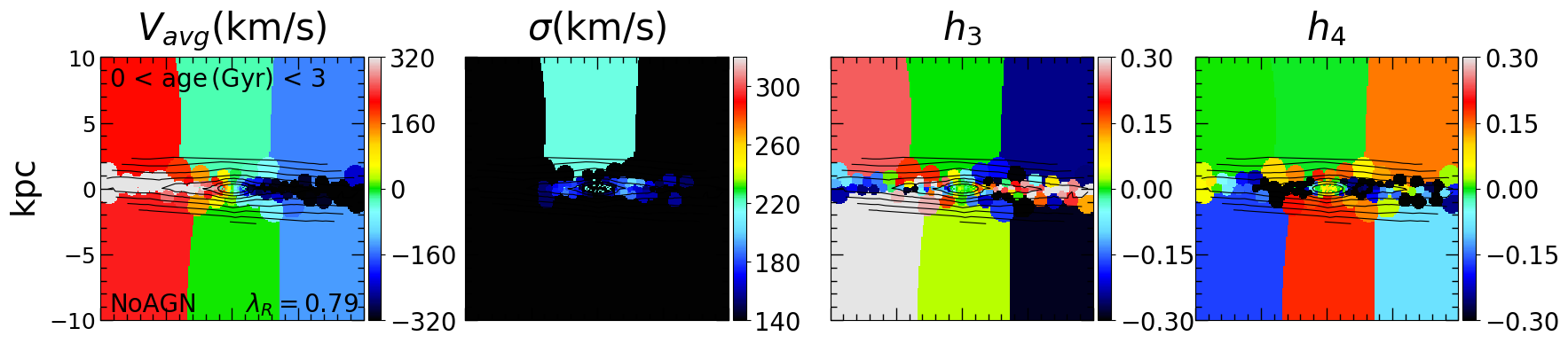
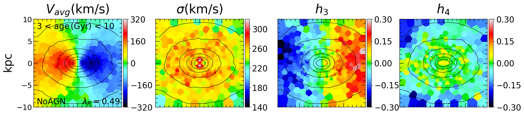
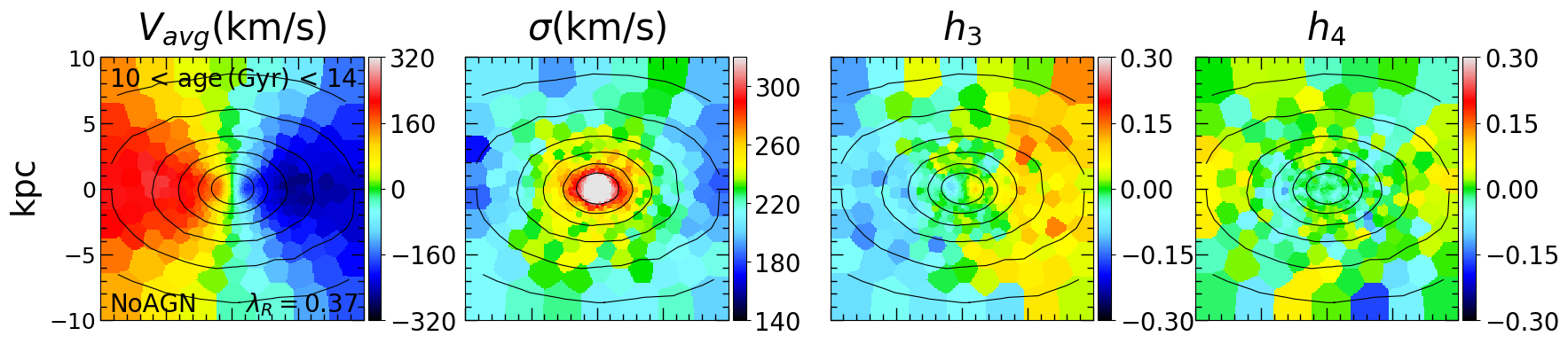
Figure 21: Kinematic maps ($V_{\rm avg}$,$\sigma$,$h_{3}$,$h_{4}$) for age-selected stellar components of galaxy 0227 simulated without AGN. From top to bottom, stars between 0 and 3 Gyr old, between 3 and 10 Gyr old, and older than 10 Gyr.

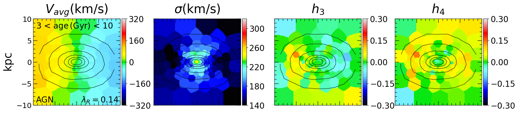
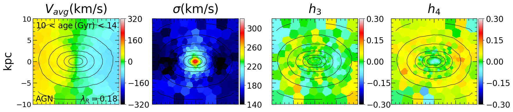
Figure 22: Kinematic maps ($V_{\rm avg}$,$\sigma$,$h_{3}$,$h_{4}$) for age-selected stellar components of galaxy 0227 simulated with AGN. From top to bottom, stars between 0 and 10 Gyr old and stars older than 10 Gyr.

References

- Aumer et al. (2013) Aumer M., White S. D. M., Naab T., Scannapieco C., 2013, MNRAS, 434, 3142
- Aumer et al. (2014) Aumer M., White S. D. M., Naab T., 2014, MNRAS, 441, 3679
- Bacon et al. (2010) Bacon R., et al., 2010, in Ground-based and Airborne Instrumentation for Astronomy III. p. 773508, doi:10.1117/12.856027
- Bailin & Steinmetz (2005) Bailin J., Steinmetz M., 2005, ApJ, 627, 647
- Bender & Moellenhoff (1987) Bender R., Moellenhoff C., 1987, A&A, 177, 71
- Bender et al. (1994) Bender R., Saglia R. P., Gerhard O. E., 1994, MNRAS, 269, 785
- Bois et al. (2010) Bois M., et al., 2010, MNRAS, 406, 2405
- Bondi (1952) Bondi H., 1952, MNRAS, 112, 195
- Bondi & Hoyle (1944) Bondi H., Hoyle F., 1944, MNRAS, 104, 273
- Brennan et al. (2018) Brennan R., Choi E., Somerville R. S., Hirschmann M., Naab T., Ostriker J. P., 2018, ApJ, 860, 14
- Bruzual & Charlot (2003) Bruzual G., Charlot S., 2003, MNRAS, 344, 1000
- Bundy et al. (2015) Bundy K., et al., 2015, ApJ, 798, 7
- Cappellari (2016) Cappellari M., 2016, ARA&A, 54, 597
- Cappellari & Copin (2003) Cappellari M., Copin Y., 2003, MNRAS, 342, 345
- Cappellari & Emsellem (2004) Cappellari M., Emsellem E., 2004, PASP, 116, 138
- Cappellari et al. (2011a) Cappellari M., Emsellem E., Krajnović D., McDermid R. M., Scott N., 2011a, MNRAS, 413, 813
- Cappellari et al. (2011b) Cappellari M., et al., 2011b, MNRAS, 413, 813
- Carpintero & Aguilar (1998) Carpintero D. D., Aguilar L. A., 1998, MNRAS, 298, 1
- Choi et al. (2012) Choi E., Ostriker J. P., Naab T., Johansson P. H., 2012, ApJ, 754, 125
- Choi et al. (2014) Choi E., Naab T., Ostriker J. P., Johansson P. H., Moster B. P., 2014, MNRAS, 442, 440
- Choi et al. (2015) Choi E., Ostriker J. P., Naab T., Oser L., Moster B. P., 2015, MNRAS, 449, 4105
- Choi et al. (2017) Choi E., Ostriker J. P., Naab T., Somerville R. S., Hirschmann M., Núñez A., Hu C.-Y., Oser L., 2017, ApJ, 844, 31
- Choi et al. (2018) Choi E., Somerville R. S., Ostriker J. P., Naab T., Hirschmann M., 2018, preprint, (arXiv:1809.02143)
- Chung & Bureau (2004) Chung A., Bureau M., 2004, AJ, 127, 3192
- Crain et al. (2015) Crain R. A., et al., 2015, MNRAS, 450, 1937
- Croom et al. (2012) Croom S. M., et al., 2012, MNRAS, 421, 872
- Croton et al. (2006) Croton D. J., et al., 2006, MNRAS, 365, 11
- Dressler (1989) Dressler A., 1989, in Osterbrock D. E., Miller J. S., eds, IAU Symposium Vol. 134, Active Galactic Nuclei. p. 217
- Dubois et al. (2013) Dubois Y., Gavazzi R., Peirani S., Silk J., 2013, MNRAS, 433, 3297
- Dubois et al. (2016) Dubois Y., Peirani S., Pichon C., Devriendt J., Gavazzi R., Welker C., Volonteri M., 2016, MNRAS, 463, 3948
- Eisenreich et al. (2017) Eisenreich M., Naab T., Choi E., Ostriker J. P., Emsellem E., 2017, MNRAS, 468, 751
- Emsellem et al. (2004) Emsellem E., et al., 2004, MNRAS, 352, 721
- Emsellem et al. (2007) Emsellem E., et al., 2007, MNRAS, 379, 401
- Emsellem et al. (2011) Emsellem E., et al., 2011, MNRAS, 414, 888
- Emsellem et al. (2014) Emsellem E., Krajnović D., Sarzi M., 2014, MNRAS, 445, L79
- Freedman & Diaconis (1981) Freedman D., Diaconis P., 1981, Zeitschrift für Wahrscheinlichkeitstheorie und Verwandte Gebiete, 57, 453
- Gebhardt et al. (2000) Gebhardt K., et al., 2000, ApJ, 539, L13
- Gerhard (1993) Gerhard O. E., 1993, MNRAS, 265, 213
- Graham et al. (2018) Graham M. T., et al., 2018, MNRAS, 477, 4711
- Guérou et al. (2016) Guérou A., Emsellem E., Krajnović D., McDermid R. M., Contini T., Weilbacher P. M., 2016, A&A, 591, A143
- Hernquist (1990) Hernquist L., 1990, ApJ, 356, 359
- Hernquist & Ostriker (1992) Hernquist L., Ostriker J. P., 1992, ApJ, 386, 375
- Hirschmann et al. (2012) Hirschmann M., Naab T., Somerville R. S., Burkert A., Oser L., 2012, MNRAS, 419, 3200
- Hirschmann et al. (2013) Hirschmann M., et al., 2013, MNRAS, 436, 2929
- Hirschmann et al. (2015) Hirschmann M., Naab T., Ostriker J. P., Forbes D. A., Duc P.-A., Davé R., Oser L., Karabal E., 2015, MNRAS, 449, 528
- Hirschmann et al. (2017) Hirschmann M., Charlot S., Feltre A., Naab T., Choi E., Ostriker J. P., Somerville R. S., 2017, preprint, (arXiv:1706.00010)
- Hoffman et al. (2009) Hoffman L., Cox T. J., Dutta S., Hernquist L., 2009, ApJ, 705, 920
- Hoyle & Lyttleton (1939) Hoyle F., Lyttleton R. A., 1939, Proceedings of the Cambridge Philosophical Society, 35, 405
- Hu et al. (2014) Hu C.-Y., Naab T., Walch S., Moster B. P., Oser L., 2014, MNRAS, 443, 1173
- Iwamoto et al. (1999) Iwamoto K., Brachwitz F., Nomoto K., Kishimoto N., Umeda H., Hix W. R., Thielemann F.-K., 1999, ApJS, 125, 439
- Jedrzejewski (1987) Jedrzejewski R. I., 1987, MNRAS, 226, 747
- Jesseit et al. (2005) Jesseit R., Naab T., Burkert A., 2005, MNRAS, 360, 1185
- Jesseit et al. (2007) Jesseit R., Naab T., Peletier R. F., Burkert A., 2007, MNRAS, 376, 997
- Jesseit et al. (2009) Jesseit R., Cappellari M., Naab T., Emsellem E., Burkert A., 2009, MNRAS, 397, 1202
- Karakas (2010) Karakas A. I., 2010, MNRAS, 403, 1413
- Kennicutt (1998) Kennicutt Jr. R. C., 1998, ApJ, 498, 541
- Kormendy (1993) Kormendy J., 1993, in Beckman J., Colina L., Netzer H., eds, The Nearest Active Galaxies. pp 197–218
- Kormendy & Ho (2013) Kormendy J., Ho L. C., 2013, ARA&A, 51, 511
- Krajnović et al. (2011) Krajnović D., et al., 2011, MNRAS, 414, 2923
- Krajnović et al. (2018) Krajnović D., Emsellem E., den Brok M., Marino R. A., Schmidt K. B., Steinmetz M., Weilbacher P. M., 2018, MNRAS, 477, 5327
- Kroupa (2001) Kroupa P., 2001, MNRAS, 322, 231
- Lagos et al. (2017) Lagos C. d. P., Schaye J., Bahe Y., van de Sande J., Kay S., Barnes D., Davis T., Dalla Vecchia C., 2017, preprint, (arXiv:1712.01398)
- Lagos et al. (2018) Lagos C. d. P., Schaye J., Bahé Y., Van de Sande J., Kay S. T., Barnes D., Davis T. A., Dalla Vecchia C., 2018, MNRAS, 476, 4327
- Lauer (1985) Lauer T. R., 1985, MNRAS, 216, 429
- Li et al. (2017) Li H., Mao S., Emsellem E., Xu D., Springel V., Krajnović D., 2017, preprint, (arXiv:1709.03345)
- Martizzi et al. (2014) Martizzi D., Jimmy Teyssier R., Moore B., 2014, MNRAS, 443, 1500
- Naab & Burkert (2001) Naab T., Burkert A., 2001, ApJ, 555, L91
- Naab & Burkert (2003) Naab T., Burkert A., 2003, ApJ, 597, 893
- Naab & Ostriker (2017) Naab T., Ostriker J. P., 2017, ARA&A, 55, 59
- Naab et al. (1999) Naab T., Burkert A., Hernquist L., 1999, ApJ, 523, L133
- Naab et al. (2006) Naab T., Jesseit R., Burkert A., 2006, MNRAS, 372, 839
- Naab et al. (2014) Naab T., et al., 2014, MNRAS, 444, 3357
- Núñez et al. (2017) Núñez A., Ostriker J. P., Naab T., Oser L., Hu C.-Y., Choi E., 2017, ApJ, 836, 204
- Oser et al. (2010) Oser L., Ostriker J. P., Naab T., Johansson P. H., Burkert A., 2010, ApJ, 725, 2312
- Oser et al. (2012) Oser L., Naab T., Ostriker J. P., Johansson P. H., 2012, ApJ, 744, 63
- Ostriker et al. (2010) Ostriker J. P., Choi E., Ciotti L., Novak G. S., Proga D., 2010, ApJ, 722, 642
- Pearson (1895) Pearson K., 1895, Proceedings of the Royal Society of London Series I, 58, 240
- Penoyre et al. (2017a) Penoyre Z., Moster B. P., Sijacki D., Genel S., 2017a, MNRAS, 468, 3883
- Penoyre et al. (2017b) Penoyre Z., Moster B. P., Sijacki D., Genel S., 2017b, MNRAS, 468, 3883
- Rodriguez-Gomez et al. (2016) Rodriguez-Gomez V., et al., 2016, MNRAS, 458, 2371
- Röttgers et al. (2014) Röttgers B., Naab T., Oser L., 2014, MNRAS, 445, 1065
- Sánchez et al. (2012) Sánchez S. F., et al., 2012, A&A, 538, A8
- Sazonov et al. (2005) Sazonov S. Y., Ostriker J. P., Ciotti L., Sunyaev R. A., 2005, MNRAS, 358, 168
- Scannapieco et al. (2005) Scannapieco C., Tissera P. B., White S. D. M., Springel V., 2005, MNRAS, 364, 552
- Scannapieco et al. (2006) Scannapieco C., Tissera P. B., White S. D. M., Springel V., 2006, MNRAS, 371, 1125
- Schaye et al. (2015) Schaye J., et al., 2015, MNRAS, 446, 521
- Schulze et al. (2018) Schulze F., Remus R.-S., Dolag K., Burkert A., Emsellem E., van de Ven G., 2018, preprint, (arXiv:1802.01583)
- Somerville & Davé (2015) Somerville R. S., Davé R., 2015, ARA&A, 53, 51
- Spergel et al. (2007) Spergel D. N., et al., 2007, ApJS, 170, 377
- Springel (2000) Springel V., 2000, MNRAS, 312, 859
- Springel (2005) Springel V., 2005, MNRAS, 364, 1105
- Thomas et al. (2007) Thomas J., Saglia R. P., Bender R., Thomas D., Gebhardt K., Magorrian J., Corsini E. M., Wegner G., 2007, MNRAS, 382, 657
- Tsatsi et al. (2017) Tsatsi A., Lyubenova M., van de Ven G., Chang J., Aguerri J. A. L., Falcón-Barroso J., Macciò A. V., 2017, preprint, (arXiv:1707.05130)
- Veale et al. (2017) Veale M., et al., 2017, MNRAS, 464, 356
- Vogelsberger et al. (2014) Vogelsberger M., et al., 2014, Nature, 509, 177
- Woosley & Weaver (1995) Woosley S. E., Weaver T. A., 1995, ApJS, 101, 181
- Wu et al. (2014) Wu X., Gerhard O., Naab T., Oser L., Martinez-Valpuesta I., Hilz M., Churazov E., Lyskova N., 2014, MNRAS, 438, 2701
- de Kool et al. (2001) de Kool M., Arav N., Becker R. H., Gregg M. D., White R. L., Laurent-Muehleisen S. A., Price T., Korista K. T., 2001, ApJ, 548, 609
- van de Sande et al. (2017) van de Sande J., et al., 2017, ApJ, 835, 104
- van der Marel & Franx (1993) van der Marel R. P., Franx M., 1993, ApJ, 407, 525