Abstract

In stochastic multi-armed bandits, the reward distribution of each arm is assumed to be stationary. This assumption is often violated in practice (e.g., in recommendation systems), where the reward of an arm may change whenever is selected, i.e., rested bandit setting. In this paper, we consider the non-parametric rotting bandit setting, where rewards can only decrease. We introduce the filtering on expanding window average (FEWA) algorithm that constructs moving averages of increasing windows to identify arms that are more likely to return high rewards when pulled once more. We prove that for an unknown horizon $T$, and without any knowledge on the decreasing behavior of the $K$ arms, FEWA achieves problem-dependent regret bound of $\widetilde{\mathcal{O}}(\log{(KT)}),$ and a problem-independent one of $\widetilde{\mathcal{O}}(\sqrt{KT})$. Our result substantially improves over the algorithm of Levine et al. (2017), which suffers regret $\widetilde{\mathcal{O}}(K^{1/3}T^{2/3})$. FEWA also matches known bounds for the stochastic bandit setting, thus showing that the rotting bandits are not harder. Finally, we report simulations confirming the theoretical improvements of FEWA.

1 Introduction

The multi-arm bandit framework (Bubeck and Cesa-Bianchi, 2012; Lattimore and Szepesvári, 2020) formalizes the exploration-exploitation dilemma in online learning, where an agent has to trade off the exploration of the environment to gather information and the exploitation of the current knowledge to maximize reward. In the stochastic setting (Thompson, 1933; Auer et al., 2002a), each arm is characterized by a stationary reward distribution. Whenever an arm is pulled, an i.i.d. sample from the corresponding distribution is observed. Despite the extensive algorithmic and theoretical study of this setting, the stationarity assumption is often too restrictive in practice, e.g., the preferences of users may change over time. The adversarial setting (Auer et al., 2002b) addresses this limitation by removing any assumption on how the rewards are generated and learning agents should be able to perform well for any arbitrary sequence of rewards. While algorithms such as Exp3 (Auer et al., 2002b) are guaranteed to achieve small regret in this setting, their behavior is conservative as all arms are repeatedly explored to avoid incurring too much regret because of unexpected changes in arms’ values. This behavior results in unsatisfactory performance in practice, where arms’ values, while non-stationary, are far from being adversarial. Garivier and Moulines (2011) proposed a variation of the stochastic setting, where the distribution of each arm is piecewise stationary. Similarly, Besbes et al. (2014) introduced an adversarial setting where the total amount of change in arms’ values is bounded. These settings fall into the restless bandit scenario, where the arms’ value evolves independently from the decisions of the agent. On the other hand, for rested bandits, the value of an arm changes only when it is pulled. For instance, the value of a service may deteriorate only when it is actually used, e.g., if a recommender system shows always the same item to the users, they may get bored (Warlop et al., 2018). Similarly, a student can master a frequently taught topic in an intelligent tutoring system and extra learning on that topic would be less effective. A particularly interesting case is represented by the rotting bandits, where the value of an arm may decrease whenever pulled. Heidari et al. (2016) studied this problem when rewards are deterministic (i.e., no noise) and showed how a greedy policy (i.e., selecting the arm that returned the largest reward the last time it was pulled) is optimal up to a small constant factor depending on the number of arms $K$ and the largest per-round decay in the arms’ value $L$. Bouneffouf and Féraud (2016) considered the stochastic setting when the dynamics of the rewards is known up to a constant factor. Finally, Levine et al. (2017) considered both non-parametric and parametric noisy rotting bandits, for which they derive algorithms with regret guarantees. In the non-parametric case, where the decrease in reward is neither constrained nor known, they introduce the sliding-window average (wSWA) algorithm, which is shown to achieve a regret to the optimal policy of order $\widetilde{\mathcal{O}}(K^{1/3}T^{2/3})$, where $T$ is the number of rounds in the experiment.

In this paper, we study the non-parametric rotting setting of Levine et al. (2017) and introduce Filtering on Expanding Window Average (FEWA) algorithm, a novel method that constructs moving average estimates of increasing windows to identify the arms that are more likely to perform well if pulled once more. Under the assumption that the reward decays are bounded, we show that FEWA achieves a regret of $\widetilde{\mathcal{O}}(\sqrt{KT})$, thus significantly improving over wSWA and matching the minimax rate of stochastic bandits up to a logarithmic factor. This shows that learning with non-increasing rewards is not more difficult than in the stationary case. Furthermore, when rewards are constant, we recover standard problem-dependent regret guarantees (up to constants), while in the rotting bandit scenario with no noise, the regret reduces to the one of Heidari et al. (2016). Numerical simulations confirm our theoretical results and show the superiority of FEWA over wSWA.

2 Preliminaries

We consider a rotting bandit scenario similar to the one of Levine et al. (2017). At each round $t$, an agent chooses an arm $i(t)\in\mathcal{K}\triangleq\mathopen{}\mathclose{{}\left\{1,...,K}\right\}$ and receives a noisy reward $r_{i(t),t}$. The reward associated to each arm $i$ is a $\sigma^{2}$-sub-Gaussian r.v. with expected value of $\mu_{i}(n)$, which depends on the number of times $n$ it was pulled before; $\mu_{i}(0)$ is the initial expected value. Let $\mathcal{H}_{t}\triangleq\mathopen{}\mathclose{{}\left\{\mathopen{}\mathclose{{}\left\{i(s),r_{i(s),s}}\right\},\forall s<t}\right\}$ be the sequence of arms pulled and rewards observed until round $t$, then

$$r_{i(t),t}\triangleq\mu_{i(t)}(N_{i(t),t})+\varepsilon_{t}\;\;\;\text{with}\;\mathop{\mathbb{E}}\mathopen{}\mathclose{{}\left[\varepsilon_{t}|\mathcal{H}_{t}}\right]=0$$

$$\text{and}\;\forall\lambda\in\mathop{\mathbb{R}},\quad\mathop{\mathbb{E}}\mathopen{}\mathclose{{}\left[e^{\lambda\varepsilon_{t}}}\right]\leq e^{\frac{\sigma\lambda^{2}}{2}},$$

where $N_{i,t}\triangleq\sum_{s=1}^{t-1}\mathbb{I}\{i(t)=i\}$ is the number of times arm $i$ is pulled before round $t$. We use $r_{i}(n)$ to denote the random reward of arm $i$ when pulled for the $n+1$-th time, i.e., $r_{i(t),t}=r_{i(t)}(N_{i(t),t})$. We introduce a non-parametric rotting assumption with bounded decay.

Assumption 1.

The reward functions $\mu_{i}$ are non-increasing with bounded decays $-L\leq\mu_{i}(n+1)-\mu_{i}(n)\leq 0.$ The initial expected value is bounded as $\mu_{i}(0)\in\mathopen{}\mathclose{{}\left[0,L}\right]$. We refer to this set of functions as $\mathcal{L}_{L}.$

The learning problem

A learning policy $\pi$ is a function from the history of observations to arms, i.e., $\pi(\mathcal{H}_{t})\in\mathcal{K}$. In the following, we often use $\pi(t)\triangleq\pi(\mathcal{H}_{t})$. The performance of a policy $\pi$ is measured by the (expected) rewards accumulated over time,

$$J_{T}(\pi)\triangleq\sum_{t=1}^{T}\mu_{\pi(t)}\mathopen{}\mathclose{{}\left(N_{\pi(t),t}}\right).$$

Since $\pi$ depends on the (random) history observed over time, $J_{T}(\pi)$ is also random. We define the expected cumulative reward as $\overline{J}_{T}(\pi)\triangleq\mathbb{E}\big{[}J_{T}(\pi)\big{]}$. We now restate a characterization of the optimal (oracle) policy.

Proposition 1 (Heidari et al., 2016).

If the expected value of each arm $\{\mu_{i}(n)\}_{i,n}$ is known, the policy $\pi^{\star}$ maximizing the expected cumulative reward $\overline{J_{T}}(\pi)$ is greedy at each round, i.e.,

$$\pi^{\star}(t)=\arg\max_{i}\mu_{i}\mathopen{}\mathclose{{}\left(N_{i,t}}\right).$$ (1)

We denote by $J^{\star}\triangleq\overline{J}_{T}(\pi^{\star})=J_{T}(\pi^{\star})$, the cumulative reward of the optimal policy.

The objective of a learning algorithm is to implement a policy $\pi$ with performance as close to $\pi^{\star}$’s as possible. We define the (random) regret as

$$R_{{\color[rgb]{0.25,0.0,0.6}T}}(\pi)\triangleq J^{\star}-J_{T}(\pi).$$ (2)

Notice that the regret is measured against an optimal allocation over arms rather than a fixed-arm policy as it is a case in adversarial and stochastic bandits. Therefore, even the adversarial algorithms that one could think of applying in our setting (e.g., Exp3 of Auer et al., 2002a) are not known to provide any guarantee for our definition of regret. On the other hand, for constant $\mu_{i}(n)$-s, our problem and definition of regret reduce to the one of standard stochastic bandits.

Let $N_{i,T}^{\star}$ be the (deterministic) number of rounds that arm $i$ is pulled by the oracle policy $\pi^{\star}$ up to round $T$ (excluded). Similarly, for a policy $\pi$, let $N_{i,T}^{\pi}$ be the (random) number pulls of arm $i$. The cumulative reward can be rewritten as

$$J_{T}(\pi) =\sum_{t=1}^{T}\sum_{i\in\mathcal{K}}\mathbb{I}_{\{\pi(t)=i\}}\mu_{i}\mathopen{}\mathclose{{}\left(N_{i,t}^{\pi}}\right)=\sum_{i\in\mathcal{K}}\sum_{s=0}^{N^{\pi}_{i,T}-1}\mu_{i}(s).$$

Then, we can conveniently rewrite the regret as

$$\!R_{{\color[rgb]{0.25,0.0,0.6}T}}(\pi) =\sum_{i\in\mathcal{K}}\mathopen{}\mathclose{{}\left(\sum_{s=0}^{N_{i,T}^{\star}-1}\mu_{i}(s)-\sum_{s=0}^{N_{i,T}^{\pi}-1}\mu_{i}(s)}\right)$$

$$=\sum_{i\in\textsc{up}}\sum_{s=N_{i,T}^{\pi}}^{N_{i,T}^{\star}-1}\mu_{i}(s)-\sum_{i\in\textsc{op}}\sum_{s=N_{i,T}^{\star}}^{N_{i,T}^{\pi}-1}\mu_{i}(s),$$ (3)

where we define $\textsc{up}\triangleq\mathopen{}\mathclose{{}\left\{i\in\mathcal{K}|N_{i,T}^{\star}>N_{i,T}^{\pi}}\right\}$ and likewise $\textsc{op}\triangleq\mathopen{}\mathclose{{}\left\{i\in\mathcal{K}|N_{i,T}^{\star}<N_{i,T}^{\pi}}\right\}$ as the sets of arms that are respectively under-pulled and over-pulled by $\pi$ w.r.t. the optimal policy.

Known regret bounds

We report existing regret bounds for two special cases. We start with the minimax regret lower bound for stochastic bandits.

Proposition 2.

(Auer et al., 2002b, Thm. 5.1) For any learning policy $\pi$ and any horizon $T$, there exists a stochastic stationary problem $\mathopen{}\mathclose{{}\left\{\mu_{i}(n)\triangleq\mu_{i}}\right\}_{i}$ with $K$ $\sigma$-sub-Gaussian arms such that $\pi$ suffers a regret

$$\mathbb{E}[R_{{\color[rgb]{0.25,0.0,0.6}T}}(\pi)]\geq\frac{\sigma}{10}\min\mathopen{}\mathclose{{}\left(\sqrt{KT},T}\right).$$

where the expectation is w.r.t. both the randomization over rewards and algorithm’s internal randomization.

Heidari et al. (2016) derived regret lower and upper bounds for deterministic rotting bandits (i.e., $\sigma=0$).

Proposition 3.

(Heidari et al., 2016, Thm. 3) For any learning policy $\pi$, there exists a deterministic rotting bandits (i.e., $\sigma=0$) satisfying Assumption 1 with bounded decay $L$ such that $\pi$ suffers an expected regret

$$\mathbb{E}[R_{{\color[rgb]{0.25,0.0,0.6}T}}(\pi)]\geq\frac{L}{2}(K-1).$$

Let $\pi^{\sigma_{0}}$ be the greedy policy that selects at each round the arm with the largest reward observed so far, i.e., $\pi^{\sigma_{0}}(t)\triangleq\operatorname*{arg\,max}_{i}(\mu_{i}(N_{i,t}-1))$. For any deterministic rotting bandits (i.e., $\sigma=0$) satisfying Assumption 1 with bounded decay $L$, $\pi^{\sigma_{0}}$ suffers an expected regret

$$\mathbb{E}[R_{{\color[rgb]{0.25,0.0,0.6}T}}(\pi^{\sigma_{0}})]\leq L(K-1).$$

Any problem in the two settings above is a rotting problem with parameters ($\sigma$, $L$). Therefore, the performance of any algorithm on the general rotting problem is also bounded by these two lower bounds.

3 FEWA: Filtering on expanding window average

Since the expected rewards $\mu_{i}$ change over time, the main difficulty in the non-parametric rotting bandits is that we cannot rely on all samples observed until round $t$ to predict which arm is likely to return the highest reward in the future. In fact, the older a sample, the less representative it is for future rewards. This suggests constructing estimates using the more recent samples. Nonetheless, discarding older rewards reduces the number of samples used in the estimates, thus increasing their variance. In Alg. 1 we introduce FEWA (or $\pi_{\rm F}$) that at each round $t$, relies on estimates using windows of increasing length to filter out arms that are suboptimal with high probability and then pulls the least pulled arm among the remaining arms.

We first describe the subroutine Filter in Alg. 2, which receives a set of active arms $\mathcal{K}_{h}$, a window $h$, and a confidence parameter $\delta$ as input and returns an updated set of arms $\mathcal{K}_{h+1}$. For each arm $i$ that has been pulled $n$ times, the algorithm constructs an estimate $\widehat{\mu}^{h}_{i}(n)$ that averages the $h\leq n$ most recent rewards observed from $i$. The subroutine Filter discards all the arms whose mean estimate (built with window $h$) from $\mathcal{K}_{h}$ is lower than the empirically best arm by more than twice a threshold $c(h,\delta_{t})$ constructed by standard Hoeffding’s concentration inequality (see Prop. 4).

Algorithm 1 FEWA

0:  $\sigma$, $\mathcal{K}$, $\alpha$, $\delta_{0}\leftarrow 1$

1:  pull each arm once, collect reward, and initialize $N_{i,K}\leftarrow 1$

2:  for $t\leftarrow K+1,K+2,\dots$ do

3:     $\delta_{t}\leftarrow\delta_{0}/(t^{\alpha})$

4:     $h\leftarrow 1$ {initialize bandwidth}

5:     $\mathcal{K}_{1}\leftarrow\mathcal{K}$ {initialize with all the arms}

6:     $i(t)\leftarrow{\tt none}$

7:     while $i(t)$ is ${\tt none}$ do

8:        $\mathcal{K}_{h+1}\leftarrow{\textsc{Filter}}(\mathcal{K}_{h},h,\delta_{t})$

9:        $h\leftarrow h+1$

10:        if $\exists i\in\mathcal{K}_{h}$ such that $N_{i,t}=h$ then

11:           $i(t)\leftarrow\arg\min_{i\in\mathcal{K}_{h}}N_{i,t}$

12:        end if

13:     end while

14:     receive $r_{i}(N_{i,t+1})\leftarrow r_{i(t),t}$

15:     $N_{i(t),t}\leftarrow N_{i(t),t-1}+1$

16:     $N_{j,t}\leftarrow N_{j,t-1},\quad\forall j\neq i(t)$

17:  end for

Algorithm 2 Filter

0:  $\mathcal{K}_{h}$, $h$, $\delta_{t}$

1:  $c(h,\delta_{t})\leftarrow\sqrt{(2\sigma^{2}/h)\log{(1/\delta_{t})}}$

2:  for $i\in\mathcal{K}_{h}$ do

3:     $\widehat{\mu}^{h}_{i}(N_{i,t})\leftarrow\frac{1}{h}\sum_{j=1}^{h}r_{i}(N_{i,t}-j)$

4:  end for

5:  $\widehat{\mu}^{h}_{\max,t}\leftarrow\max_{i\in\mathcal{K}_{h}}\widehat{\mu}^{h}_{i}(N_{i,t})$

6:  for $i\in\mathcal{K}_{h}$ do

7:     $\Delta_{i}\leftarrow\widehat{\mu}^{h}_{\max,t}-\widehat{\mu}^{h}_{i}(N_{i,t})$

8:     if $\Delta_{i}\leq 2c(h,\delta_{t})$ then

9:        add $i$ to $\mathcal{K}_{h+1}$

10:     end if

11:  end for

11:  $\mathcal{K}_{h+1}$

The Filter subroutine is used in FEWA to incrementally refine the set of active arms, starting with a window of size $1$, until the condition at Line 10 is met. As a result, $\mathcal{K}_{h+1}$ only contains arms that passed the filter for all windows from $1$ up to $h$. Notice that it is important to start filtering arms from a small window and to keep refining the previous set of active arms. In fact, the estimates constructed using a small window use recent rewards, which are closer to the future value of an arm. As a result, if there is enough evidence that an arm is suboptimal already at a small window $h$, it should be directly discarded. On the other hand, a suboptimal arm may pass the filter for small windows as the threshold $c(h,\delta_{t})$ is large for small $h$ (i.e., as few samples are used in constructing $\widehat{\mu}^{h}_{i}(N_{i,t})$, the estimation error may be high). Thus, FEWA keeps refining $\mathcal{K}_{h}$ for larger windows in the attempt of constructing more accurate estimates and discard more suboptimal arms. This process stops when we reach a window as large as the number of samples for at least one arm in the active set $\mathcal{K}_{h}$ (i.e., Line 10). At this point, increasing $h$ would not bring any additional evidence that could refine $\mathcal{K}_{h}$ further (recall that $\widehat{\mu}^{h}_{i}(N_{i,t})$ is not defined for $h>N_{i,t}$). Finally, FEWA selects the active arm $i(t)$ whose number of samples matches the current window, i.e., the least pulled arm in $\mathcal{K}_{h}$. The set of available rewards and the number of pulls are then updated accordingly.

Runtime and memory usage At each round $t$, FEWA needs to store and update up to $t$ averages per-arm. Since moving from an average computed on window $h$ to $h+1$ can be done incrementally at a cost $\mathcal{O}(1)$, the worst-case time and memory complexity per round is $\mathcal{O}(Kt)$, which amounts to a total $\mathcal{O}(KT^{2})$ cost. This is not practical for large $T$. We have a fix.

In App. E we detail EFF-FEWA, an efficient variant of FEWA. EFF-FEWA is built around two main ideas. First, at any round $t$ we can avoid calling Filter for all possible windows $h$ starting from 1 with an increment of 1. In fact, the confidence interval $c(h,\delta_{t})$ decreases as $1/\sqrt{h}$ and we could select windows $h$ with an exponential increment so that confidence intervals between two consecutive calls to Filter have a constant ratio. In practice, we replace the window increment (Line 9 of FEWA) by a geometric window $h\triangleq 2^{j}$. This modification alone is not enough to reduce the computation. While we reduce the number of estimates that we construct, updating $\widehat{\mu}^{h}_{i}$ from $h=2^{j}$ to $h=2^{j+1}$ still requires spanning over past samples, thus leading to the same $\mathcal{O}(Kt)$ complexity in the worst-case. In order to reduce the overall complexity, we avoid recomputing $\widehat{\mu}^{h}_{i}$ at each call of Filter and by replacing it with precomputed estimates. Whenever $N_{i,t}=2^{j}$ for some $j$, we create an estimate $\widehat{s}_{i,j}^{\,c}$ by averaging all the last $N_{i,t}$ samples. These estimates are then used whenever Filter is called with $h=2^{j}$. Instead of updating $\widehat{s}_{i,j}^{\,c}$ at each new sample, we create an associated pending estimate $\widehat{s}_{i,j}^{\,p}$ which averages all the more recent samples. More formally, let $t$ be the round when $N_{i,t}=2^{j}$, then $\widehat{s}_{i,j}^{\,p}$ is initialized at 0 and it then stores the average of all the samples observed from $t$ to $t^{\prime}$, when $N_{i,t^{\prime}}=2^{j+1}$ (i.e., $\widehat{s}_{i,j}^{\,p}$ is averaging at most $2^{j}$ samples). At this point, the $2^{j}$ samples averaged in $\widehat{s}_{i,j}^{\,c}$ are outdated and they are replaced by the new average $\widehat{s}_{i,j}^{\,p}$, which is then reinitialized to 0. The sporadic update of the precomputed estimates and the small number of them drastically reduces per-round time and space complexity to $\mathcal{O}(K\log t)$. Furthermore, EFF-FEWA preservers the same regret guarantees as FEWA. In the worst case, $\widehat{s}_{i,j}^{\,c}$ may not cover the last $2^{j-1}-1$ samples. Nonetheless, the precomputed estimates with smaller windows (i.e., $j^{\prime}<j$) are updated more frequently, thus effectively covering the $2^{j-1}-1$ samples “missed” by $\widehat{s}_{i,j}^{\,c}$. As a result, the active sets returned by Filter are still accurate enough to derive regret guarantees that are only a constant factor worse than FEWA (App. E).

4 Regret Analysis

We first give problem-independent regret bound for FEWA and sketch its proof in Sect. 4.1. Then, we derive problem-dependent guarantees in Sect. 4.2.

Theorem 1.

For any rotting bandit scenario with means $\{\mu_{i}(n)\}_{i,n}$ satisfying Asm. 1 with bounded decay $L$ and any horizon $T$, FEWA run with $\alpha=5$, i.e., $\delta_{t}=1/t^{5},$ suffers an expected regret  of

$$\mathbb{E}[R_{{\color[rgb]{0.25,0.0,0.6}T}}(\pi_{\rm F})]\leq 13\sigma(\sqrt{KT}+K)\sqrt{\log(T)}+2KL.$$

Comparison to Levine et al. (2017)

The regret of wSWA is bounded by $\widetilde{\mathcal{O}}(\mu_{\max}^{1/3}K^{1/3}T^{2/3})$ for rotting functions with range in $[0,\mu_{\max}]$. In our setting, we do not restrict rewards to stay positive but we bound the per-round decay by $L$, thus leading to rotting functions with range in $\mathopen{}\mathclose{{}\left[-LT,L}\right]$. As a result, when applying wSWA to our setting, we should set $\mu_{\max}=L(T+1)$, which leads to $\mathcal{O}(T)$ regret, thus showing that according to its original analysis, wSWA may not be able to learn in our general setting. On the other hand, we could use FEWA in the setting of Levine et al. (2017) by setting $L=\mu_{\max}$ as the largest drop that could occur. In this case, FEWA suffers a regret of $\widetilde{\mathcal{O}}(\sqrt{KT})$, thus significantly improving over wSWA. The improvement is mostly due to the fact that FEWA exploits filters using moving averages with increasing windows to discard arms that are suboptimal w.h.p. Since this process is done at each round, FEWA smoothly tracks changes in the value of each arm, so that if an arm becomes worse later on, other arms would be recovered and pulled again. On the other hand, wSWA relies on a fixed exploratory phase where all arms are pulled in a round-robin way and the tracking is performed using averages constructed with a fixed window. Moreover, FEWA is anytime, while the fixed exploratory phase of wSWA requires either to know $T$ or to resort to a doubling trick, which often performs poorly in practice.

Comparison to deterministic rotting bandits

For $\sigma=0$, our upper bound reduces to $KL$, thus matching the prior (upper and lower) bound of Heidari et al. (2016) for deterministic rotting bandits. Moreover, the additive decomposition of regret shows that there is no coupling between the stochastic problem and the rotting problem as terms depending on the noise level $\sigma$ are separated from the terms depending on the rotting level $L$, while in wSWA these are coupled by a $L^{1/3}\sigma^{2/3}$ factor in the leading term.

Comparison to stochastic bandits

The regret of FEWA matches the worst-case optimal regret bound of the standard stochastic bandits (i.e., $\mu_{i}(n)$s are constant) up to a logarithmic factor. Whether an algorithm can achieve $\mathcal{O}(\sqrt{KT})$ regret bound is an open question. On one hand, FEWA needs confidence bounds to hold for different windows at the same time, which requires an additional union bound and thus larger confidence intervals w.r.t. UCB1. On the other hand, our worst-case analysis shows that some of the difficult problems that reach the worst-case bound of Thm. 1 are realized with constant functions, which is the standard stochastic bandits, for which MOSS-like (Audibert and Bubeck, 2009) algorithms achieve regret guarantees without the $\log T$ factor. Thus, the necessity of the extra $\log T$ factor for the worst-case regret of rotting bandits remains an open problem.

4.1 Sketch of the proof

We now give a sketch of the proof of our regret bound. We first introduce the expected value of the estimators used in FEWA. For any $n$ and $1\leq h\leq n$, we define

$$\overline{\mu}^{h}_{i}(n)\triangleq\mathop{\mathbb{E}}\mathopen{}\mathclose{{}\left[\widehat{\mu}^{h}_{i}(n)}\right]=\frac{1}{h}\sum_{j=1}^{h}\mu_{i}(n-j).$$

Notice that at round $t$, if the number of pulls of arm $i$ is $N_{i,t}$, then $\overline{\mu}^{1}_{i}(N_{i,t})=\mu_{i}(N_{i,t}-1)$, which is the expected value of arm $i$ the last time it was pulled. We introduce Hoeffding’s concentration inequality and the favorable event that we leverage in the analysis.

Proposition 4.

For any fixed arm $i$, number of pulls $n$, and window $h$, we have that with probability $1-\delta,$

$$\big{|}\widehat{\mu}^{h}_{i}(n)-\overline{\mu}^{h}_{i}(n)\big{|}\leq c(h,\delta)\triangleq\sqrt{\frac{2\sigma^{2}}{h}\log{\frac{1}{\delta}}}\cdot$$ (4)

For any round $t$ and confidence $\delta_{t}\triangleq\delta_{0}/t^{\alpha}$, let

$$\!\xi_{t}\!\triangleq\!\Big{\{} \forall i\in\mathcal{K},\forall n\leq t,\forall h\leq n,\big{|}\widehat{\mu}^{h}_{i}(n)-\overline{\mu}^{h}_{i}(n)\big{|}\!\leq\!c(h,\delta_{t})\!\Big{\}}$$

be the event under which the estimates constructed by FEWA at round $t$ are all accurate up to $c(h,\delta_{t})$. Taking a union bound gives $\mathbb{P}(\xi_{t})\geq 1-Kt^{2}\delta_{t}/2.$

Active set

We derive an important lemma that provides support for the arm selection process obtained by a series of refinements through the Filter subroutine. Recall that at any round $t$, after pulling arms $\{N^{\pi_{\rm F}}_{i,t}\}_{i}$ the greedy (oracle) policy would select an arm

$$i^{\star}_{t}\mathopen{}\mathclose{{}\left(\mathopen{}\mathclose{{}\left\{N^{\pi_{\rm F}}_{i,t}}\right\}_{i}}\right)\in\operatorname*{arg\,max}_{i\in\mathcal{K}}\mu_{i}\mathopen{}\mathclose{{}\left(N^{\pi_{\rm F}}_{i,t}}\right).$$

We denote by $\mu^{+}_{t}(\pi_{\rm F})\triangleq\max_{i\in\mathcal{K}}\mu_{i}(N^{\pi_{\rm F}}_{i,t}),$ the reward obtained by pulling $i^{\star}_{t}.$ The dependence on $\pi_{\rm F}$ in the definition of $\mu^{+}_{t}(\pi_{\rm F})$ stresses the fact that we consider what the oracle policy would do at the state reached by $\pi_{\rm F}$. While FEWA cannot directly match the performance of the oracle arm, the following lemma shows that the reward averaged over the last $h$ pulls of any arm in the active set is close to the performance of the oracle arm up to four times $c(h,\delta_{t})$.

Lemma 1.

On the favorable event $\xi_{t}$, if an arm $i$ passes through a filter of window $h$ at round $t$, i.e., $i\in\ \mathcal{K}_{h}$, then the average of its $h$ last pulls satisfies

$$\overline{\mu}^{h}_{i}(N_{i,t}^{\pi_{\rm F}})\geq\mu^{+}_{t}(\pi_{\rm F})-4c(h,\delta_{t}).$$ (5)

This result relies heavily on the non-increasing assumption of rotting bandits. In fact, for any arm $i$ and any window $h$, we have

$$\overline{\mu}_{i}^{h}(N_{i,t}^{\pi_{\rm F}})\geq\overline{\mu}_{i}^{1}(N_{i,t}^{\pi_{\rm F}})\geq\mu_{i}(N_{i,t}^{\pi_{\rm F}}).$$

While the inequality above for $i_{t}^{*}$ trivially satisfies Eq. 5, Lem. 1 is proved by integrating the possible errors introduced by the filter in selecting active arms due to the error of the empirical estimates.

Relating FEWA to the oracle policy

While Lem. 1 provides a link between the value of the arms returned by the filter and the oracle arm, $i^{\star}_{t}$ is defined according to the number of pulls obtained by FEWA up to $t$, which may significantly differ from the sequence of pulls of the oracle policy. In order to bound the regret, we need to relate the actual performance of the optimal policy to the value of the arms pulled by FEWA. Let $h_{i,t}\triangleq\mathopen{}\mathclose{{}\left|N_{i,t}^{\pi_{\rm F}}-N_{i,t}^{\star}}\right|$ be the absolute difference in the number of pulls between $\pi_{\rm F}$ and the optimal policy up to $t$. Since $\sum_{i}N_{i,t}^{\pi_{\rm F}}=\sum_{i}N_{i,t}^{\star}=t$, we have that $\sum_{i\in{\textsc{op}}}h_{i,t}=\sum_{i\in{\textsc{up}}}h_{i,t}$ which means that there are as many total overpulls as underpulls. Let $j\in\textsc{up}$ be an underpulled arm with $N_{j,T}^{\pi_{\rm F}}<N_{j,T}^{\star}$, then, for all $s\in\mathopen{}\mathclose{{}\left\{0,\ldots,h_{j,t}}\right\}$, we have the inequality

$$\mu^{+}_{T}(\pi_{\rm F}) =\max_{i\in\mathcal{K}}\mu_{i}(N_{i,T}^{\pi_{\rm F}})\geq\mu_{j}(N_{j,T}^{\pi_{\rm F}}+s).$$ (6)

As a result, from Eq. 3 we have the regret upper bound

$$R_{{\color[rgb]{0.25,0.0,0.6}T}}(\pi_{\rm F})\leq\sum_{i\in\textsc{op}}\sum_{h=0}^{h_{i,T}-1}\mathopen{}\mathclose{{}\left(\mu^{+}(\pi_{\rm F})-\mu_{i}(N_{i,T}^{\pi^{\star}}+h)}\right),$$ (7)

where we have obtained the inequality by bounding $\mu_{i}(t^{\prime})\leq\mu^{+}_{T}(\pi_{\rm F})$ in the first summation and then using $\sum_{i\in{\textsc{op}}}h_{i,T}=\sum_{i\in{\textsc{up}}}h_{i,T}$. While the previous expression shows that we can just focus on over-pulled arms in op, it is still difficult to directly control the expected reward $\mu_{i}(N_{i,T}^{\pi^{\star}}+h)$, as it may change at each round (by at most $L$). Nonetheless, we notice that its cumulative sum can be directly linked to the average of the expected reward over a suitable window. In fact, for any $i\in\textsc{op}$ and $h_{i,T}\geq 2$, we have

$$(h_{i,T}-1)\overline{\mu}^{h_{i,T}-1}_{i}(N_{i,T}-1)=\sum_{t^{\prime}=0}^{h_{i,T}-2}\mu_{i}(N_{i,T}^{\pi^{\star}}+t^{\prime}).$$

At this point we can control the regret for each $i\in\textsc{op}$ in Eq. 7 by applying the following corollary of Lem. 1.

Corollary 1.

Let $i\in\textsc{op}$ be an arm overpulled by FEWA at round $t$ and $h_{i,t}\triangleq N_{i,t}^{\pi_{\rm F}}-N_{i,t}^{\pi^{\star}}\geq 1$ be the difference in the number of pulls w.r.t. the optimal policy $\pi^{\star}$ at round $t$. On the favorable event $\xi_{t}$, we have

$$\mu^{+}_{t}(\pi_{\rm F})-\overline{\mu}^{h_{i,t}}_{i}(N_{i,t})\leq 4c(h_{i,t},\delta_{t}).$$ (8)

4.2 Problem-dependent guarantees

Since our setting generalizes the standard stochastic bandit setting, a natural question is whether we pay any price for this generalization. While the result of Levine et al. (2017) suggested that learning in rotting bandits could be more difficult, in Thm. 1 we actually proved that FEWA nearly matches the problem-independent regret $\widetilde{\mathcal{O}}(\sqrt{KT})$. We may wonder whether this is true for the problem-dependent regret as well.

Remark 1.

Consider a stationary stochastic bandit setting with expected rewards $\{\mu_{i}\}_{i}$ and $\mu_{\star}\triangleq\max_{i}\mu_{i}$. Corollary 1 guarantees that for $\delta_{t}\geq 1/T^{\alpha},$

$$\mu_{\star}-\mu_{i}\leq 4c\mathopen{}\mathclose{{}\left(h_{i,T}-1,\delta_{t}}\right)=4\sqrt{\frac{2\alpha\sigma^{2}\log(T)}{h_{i,T}-1}}$$

$$\text{\ or equivalently,\ }h_{i,T}\leq 1+\frac{32\alpha\sigma^{2}\log(T)}{(\mu_{\star}-\mu_{i})^{2}}\cdot$$ (9)

Therefore, our algorithm matches the lower bound of Lai and Robbins (1985) up to a constant, thus showing that learning in the rotting bandits are never harder than in the stationary case. Moreover, this upper bound is at most $\alpha$ larger than the one for UCB1 (Auer et al., 2002a). The main source of suboptimality is the use of a confidence bound filtering instead of an upper-confidence index policy. Selecting the less pulled arm in the active set is conservative as it requires uniform exploration until elimination, resulting in a factor 4 in the confidence bound guarantee on the selected arm (vs. 2 for UCB), which implies 4 times more overpulls than UCB (see Eq. 9). We conjecture that this may not be necessarily needed and it is an open question whether it is possible to derive either an index policy or a better selection rule. The other source of suboptimality w.r.t. UCB is the use of larger confidence bands because of the higher number of estimators computed at each round ($Kt^{2}$ instead of $Kt$ for UCB).

Remark 1 also reveals that Corollary 1 can be used to derive a general problem-dependent result in the rotting case. In particular, with Corollary 1 we upper-bound the maximum number of overpulls by a problem dependent quantity

$$h_{i,T}^{+}\triangleq\max\mathopen{}\mathclose{{}\left\{h\leq 1+\frac{32\alpha\sigma^{2}\log(T)}{\Delta_{i,h-1}^{2}}}\right\}\mathbin{\raisebox{2.15277pt}{,}}$$ (10)

$$\text{\qquad where \ }\Delta_{i,h}\triangleq\min_{j\in\mathcal{K}}\mu_{j}\mathopen{}\mathclose{{}\left(N_{j,T}^{\star}-1}\right)-\overline{\mu}_{i}^{h}\mathopen{}\mathclose{{}\left(N_{i,t}^{\star}+h}\right).$$

We then use Corollary 1 again to upper-bound the regret caused by $h_{i,T}^{+}$ overpulls for each arm, leading to Theorem 2 (see the full proof in App. D).

Theorem 2.

For $\alpha=5$ and $C_{\alpha}\triangleq 32\alpha\sigma^{2}$, the regret of FEWA is bounded as

$$\mathbb{E}\mathopen{}\mathclose{{}\left[R_{T}(\pi_{\rm F})}\right]\leq\sum_{i\in\mathcal{K}}\mathopen{}\mathclose{{}\left(\frac{C_{5}\log(T)}{\Delta_{i,h_{i,T}^{+}-1}}+\sqrt{C_{5}\log(T)}+2L}\right).$$

5 Numerical simulations

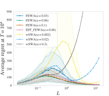
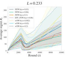
Figure 1: Comparison between FEWA and wSWA in the 2-arm setting. Left: Regret at $T=10000$ for different values of $L$. Middle-right: Regret over time for $L=0.23$ (worst case for FEWA) and $L=4.24$ (case of $L\gg\sigma$). We highlight the $\mathopen{}\mathclose{{}\left[10\%,90\%}\right]$ confidence region.

2-arms

We design numerical simulations to study the difference between wSWA and FEWA. We consider rotting bandits with two arms defined as

$$\mu_{1}(n)=0,\;\;\forall n\leq T\quad\text{and}\quad\mu_{2}(n)=\begin{cases}\frac{L}{2}&\text{ if }n<\frac{T}{4}\mathbin{\raisebox{2.15277pt}{,}}\\ -\frac{L}{2}&\text{ if }n\geq\frac{T}{4}\cdot\end{cases}$$

The rewards are then generated by applying a Gaussian i.i.d. noise $\mathcal{N}\mathopen{}\mathclose{{}\left(0,\sigma=1}\right)$. The single point of non-stationarity in the second arm is designed to satisfy Asm. 1 with a bounded decay $L$. It is important to notice that in this specific case, $L$ also plays the role of defining the gap $\Delta$ between the arms, which is known to heavily impact the performance both in stochastic bandits and in the rotting bandits (Cor. 2). In particular, for any learning strategy, the gap between the two arms is always $\Delta=|\mu_{1}(n_{1})-\mu_{2}(n_{2})|=L/2$. Recall that in stochastic bandits, the problem independent bound $\mathcal{O}(\sqrt{KT})$ is obtained by the worst-case choice of $\Delta\triangleq\sqrt{K/T}$. In the two-arm setting defined above, the optimal allocation is $N_{1,T}^{\star}=3T/4$ and $N_{2,T}^{\star}=T/4$.

Algorithms

Both algorithms have a parameter $\alpha$ to tune. In wSWA, $\alpha$ is a multiplicative constant to tune the window. We test three different values of $\alpha$, including the recommendation of Levine et al. (2017), $\alpha=0.2$. In general, the smaller the $\alpha$, the smaller the averaging window and the more reactive the algorithm is to large drops. Nonetheless, in stationary regimes, this may correspond to high variance and poor regret. On the other hand, a large value of $\alpha$ may reduce variance but increase the bias in case of rapidly rotting arms. Thm. 3.1 of Levine et al. (2017) reveals this trade-off in the regret bound of wSWA, which has a factor $(\alpha\mu_{\max}+\alpha^{-1/2})$, where $\mu_{\max}$ is the largest arm value. The best choice of $\alpha$ is then $\mu_{\max}^{-2/3}$, which reduces the previous constant to $\mu_{\max}^{1/3}$. In our experiment, $\mu_{\max}=L$ and we could expected that for any fixed $\alpha$, wSWA may perform well in cases when $\alpha\approx\mu_{\max}^{-2/3}$, while the performance may degrade for larger $\mu_{\max}$.

In FEWA, $\alpha$ tunes the confidence $\delta_{t}=1/(t^{\alpha})$ used in $c(h,\delta_{t})$. While our analysis suggests $\alpha=5$, the analysis of confidence intervals, union bounds, and filtering algorithms is too conservative. Therefore, we use more aggressive values, $\alpha\in\mathopen{}\mathclose{{}\left\{0.03,0.06,0.1}\right\}.$

Experiments

In Fig. 1, we compare the performance of the two algorithms and their dependence on $L$. The first plot shows the regret at $T$ for various values of $L$. The second and the third plot show the regret as a function of $T$ for $L=0.23$ and $L=4.24$, which corresponds to the worst empirical performance for FEWA and to the $L\gg\sigma$ regime respectively. All experiments have $T=10000$ and are averaged over $500$ runs.

Before discussing the results, we point out that in the rotting setting, the regret can increase and decrease over time. Consider two simple policies: $\pi_{1}$, which first pulls arm $1$ for $N^{\star}_{1,T}$ times and then arm $2$ for $N^{\star}_{2,T}$ times, and $\pi_{2}$ in reversed order (first arm $2$ and then arm $1$). If we take $\pi_{2}$ as reference, $\pi_{1}$ has an increasing regret for the first $T/4$ rounds, which then would plateau from $T/4$ up to $3T/4$ as both $\pi_{1}$ and $\pi_{2}$ are pulling arm $1$. Then from $3T/4$ to $T$, the regret of $\pi_{1}$ would reverse back to 0 since $\pi_{2}$ would keep selecting arm $1$ and getting a reward of $0$, while $\pi_{1}$ transitions to pulling arm $2$ with a reward of $L/2$.

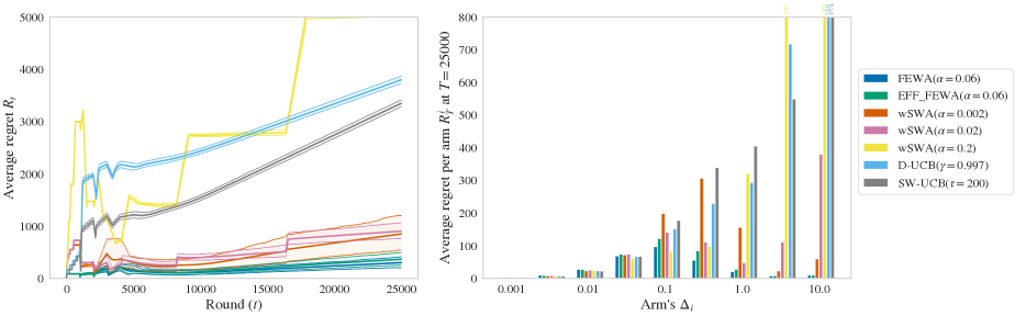
Figure 2: 10-arm setting. Left: Regret over time. Right: Regret per arm at the end of the experiment.

Results

Fig. 1 shows that the performance of wSWA depends on the proper tuning of $\alpha$ w.r.t. $\mu_{\max}=L$, as predicted by Thm. 3.1 of Levine et al. (2017). In fact, for small values of $L$, the best choice is $\alpha=0.2$, while for larger values of $L$ a smaller $\alpha$ is preferable. In particular, when $L$ grows very large, the regret tends to grow linearly with $L$. On the other hand, FEWA seems much more robust to different values of $L$. Whenever $T$ and $\sigma$ are large compared to $L$, Thm. 1 suggests that the regret of FEWA is dominated by $\mathcal{O}(\sigma\sqrt{KT})$, while the term $KL$ becomes more relevant for large values of the drop $L$. We also notice that since $L$ defines the gap between the value of $\mu_{1}$ and $\mu_{2}$, the problem-independent bound is achieved for the worst-case choice of $L\sim 2\sqrt{K/T}$, when the regret of FEWA is indeed the largest. Fig. 1 middle and right confirm these findings for the extreme choice of the worst-case value of $L$ and the regime where the drop is much larger than the noise level, i.e., where the term $KL$ dominates the regret.

We conclude that FEWA is more robust than wSWA as it almost always achieves the best performance across different problems while being agnostic to the value of $L$. On the other hand, wSWA’s performance is very sensitive to the choice of $\alpha$ and the same value of the parameter may correspond to significantly different performance depending on $L$. Finally, we notice that EFF-FEWA has a regret comparable to FEWA.

10-arms

We also tested a rotting setting with 10 arms. The mean of 1 arm is constant with value 0 while the means of 9 arms abruptly decrease after 1000 pulls from $+\Delta_{i}$ to $-\Delta_{i}$. $\Delta_{i}$ is ranging from 0.001 to 10 in a geometric sequence. In this setting, the regret can be written as $R_{T}(\pi)=\sum_{i=1}^{9}h_{i,T}\Delta_{i}$. Hence, the regret per arm is $R_{T}^{i}(\pi)\triangleq\Delta_{i}h_{i,T}$. In Fig. 2, we compare the performance of different algorithms for their best parameter. The left plot shows the average regret as a function of time. The right plot shows the regret per arm (indexed by $\Delta_{i}$) at the end of the experiment.

Results

On Fig. 2 (left), we see that FEWA outperforms wSWA. On the right, we remark that no tuning of wSWA is able to perfom well for all $\Delta_{i}$s. It is comparable with the 2-arms experiments where no tuning is good on all the experiments. We also test SW-UCB and D-UCB (Garivier and Moulines, 2011) with parameters tuned for this experiment. While the two algorithms are known benchmarks for non-stationary restless bandits, they are penalized in our rested bandits problem. Indeed, they keep exploring arms that have not been pulled for many rounds which is detrimental in our case as the arms stay constant when they are not pulled. Hence, there is no good choice for their forgetting parameters: A fast forgetting rate makes the policies repeatedly pull bad arms (whose mean rewards do not change when they are not pulled in the rested setting) while a slow forgetting rate makes the policies not able to adapt to abrupt shifts.

Last, we remark that EFF-FEWA is penalized for arms with small $\Delta_{i}$, for which the impact of the delay is more significant. At the end of the game, EFF-FEWA suffers $22\%$ more regret but reduce the computational time by $99.7\%$ (Table 1).

​FEWA ​	​EFF-FEWA ​	​wSWA ​	​SW-UCB ​	​D-UCB ​
2271	7	1	5	2

Table 1: Average running time for the 10-arms experiment in seconds.

6 Conclusion

We introduced FEWA, a novel algorithm for the non-parametric rotting bandits. We proved that FEWA achieves an $\widetilde{\mathcal{O}}(\sqrt{KT})$ regret without any knowledge of the decays by using moving averages with a window that effectively adapts to the changes in the expected rewards. This result greatly improves over the wSWA algorithm by Levine et al. (2017), that suffers a regret of order $\widetilde{\mathcal{O}}(K^{1/3}T^{2/3})$. Thus our result shows that the rotting bandit scenario is not harder than the stochastic one. Our technical analysis of FEWA hinges on the adaptive nature of the window size. The most interesting aspect of the proof technique is that confidence bounds are used not only for the action selection but also for the data selection, i.e., to identify the best window to trade off the bias and the variance in estimating the current value of each arm.

Acknowledgements

We thank Nir Levine for his helpful remarks and Lilian Besson for his bandits package (Besson, 2018). The research presented was supported by European CHIST-ERA project DELTA, French Ministry of Higher Education and Research, Nord-Pas-de-Calais Regional Council, Inria and Otto-von-Guericke-Universität Magdeburg associated-team north-European project Allocate, and French National Research Agency projects ExTra-Learn (n.ANR-14-CE24-0010-01) and BoB (n.ANR-16-CE23-0003). The work of A. Carpentier is also partially supported by the Deutsche Forschungsgemeinschaft (DFG) Emmy Noether grant MuSyAD (CA 1488/1-1), by the DFG - 314838170, GRK 2297 MathCoRe, by the DFG GRK 2433 DAEDALUS, by the DFG CRC 1294 Data Assimilation, Project A03, and by the UFA-DFH through the French-German Doktorandenkolleg CDFA 01-18. This research has also benefited from the support of the FMJH Program PGMO and from the support to this program from Criteo. Part of the computational experiments were conducted using the Grid’5000 experimental testbed (https://www.grid5000.fr).

Appendix A Proof of core FEWA guarantees

See 1

Proof.

Let $i$ be an arm that passed a filter of window $h$ at round $t$. First, we use the confidence bound for the estimates and we pay the cost of keeping all the arms up to a distance $2c(h,\delta_{t})$ of $\widehat{\mu}^{h}_{\max,t}$,

$$\overline{\mu}^{h}_{i}(N_{i,t})\geq\widehat{\mu}^{h}_{i}(N_{i,t})-c(h,\delta_{t})\geq\widehat{\mu}^{h}_{\max,t}-3c(h,\delta_{t})\geq\max_{i\in\mathcal{K}_{h}}\overline{\mu}^{h}_{i}(N_{i,t})-4c(h,\delta_{t}),$$ (11)

where in the last inequality, we used that for all $i\in\mathcal{K}_{h},$

$$\widehat{\mu}^{h}_{\max,t}\geq\widehat{\mu}^{h}_{i}(N_{i,t})\geq\overline{\mu}^{h}_{i}(N_{i,t})-c(h,\delta_{t}).$$

Second, since the means of arms are decaying, we know that

$$\mu^{+}_{t}(\pi_{\rm F})\triangleq\mu_{i^{\star}_{t}}(N_{i^{\star}_{t},t})\leq\mu_{i^{\star}_{t}}(N_{i^{\star}_{t},t}-1)=\overline{\mu}^{1}_{i^{\star}_{t}}(N_{i^{\star}_{t},t})\leq\max_{i\in\mathcal{K}}\overline{\mu}^{1}_{i}(N_{i,t})=\max_{i\in\mathcal{K}_{1}}\overline{\mu}^{1}_{i}(N_{i,t}).$$ (12)

Third, we show that the largest average of the last $h^{\prime}$ means of arms in $\mathcal{K}_{h^{\prime}}$ is increasing with $h^{\prime}$,

$$\forall h^{\prime}\leq N_{i,t}-1,\max_{i\in\mathcal{K}_{h^{\prime}+1}}\overline{\mu}^{h^{\prime}+1}_{i}(N_{i,t})\geq\max_{i\in\mathcal{K}_{h^{\prime}}}\overline{\mu}^{h^{\prime}}_{i}(N_{i,t}).$$

To show the above property, we remark that thanks to our selection rule, the arm that has the largest average of means, always passes the filter. Formally, we show that $\operatorname*{arg\,max}_{i\in\mathcal{K}_{h^{\prime}}}\overline{\mu}^{h^{\prime}}_{i}(N_{i,t})\subseteq\mathcal{K}_{h^{\prime}+1}.$ Let $i^{h^{\prime}}_{\max}\in\operatorname*{arg\,max}_{i\in\mathcal{K}_{h^{\prime}}}\overline{\mu}^{h^{\prime}}_{i}(N_{i,t})$. Then for such $i^{h^{\prime}}_{\max}$, we have

$$\widehat{\mu}^{h^{\prime}}_{i^{h^{\prime}}_{\rm max}}(N_{i^{h^{\prime}}_{\max},t})\geq\overline{\mu}^{h^{\prime}}_{i^{h^{\prime}}_{\max}}(N_{i^{h^{\prime}}_{\max},t})-c(h^{\prime},\delta_{t})\geq\overline{\mu}^{h^{\prime}}_{\max,t}-c(h^{\prime},\delta_{t})\geq\widehat{\mu}^{h^{\prime}}_{\max,t}-2c(h^{\prime},\delta_{t}),$$

where the first and the third inequality are due to confidence bounds on estimates, while the second one is due to the definition of $i^{h^{\prime}}_{\rm max}$.

Since the arms are decaying, the average of the last $h^{\prime}+1$ mean values for a given arm is always greater than the average of the last $h^{\prime}$ mean values and therefore,

$$\max_{i\in\mathcal{K}_{h^{\prime}}}\overline{\mu}^{h^{\prime}}_{i}(N_{i,t})=\overline{\mu}^{h^{\prime}}_{i^{h^{\prime}}_{\rm max}}(N_{i^{h^{\prime}}_{\rm max},t})\leq\overline{\mu}^{h^{\prime}+1}_{i^{h^{\prime}}_{\rm max}}(N_{i^{h^{\prime}}_{\rm max},t})\leq\max_{i\in\mathcal{K}_{h^{\prime}+1}}\overline{\mu}^{h^{\prime}+1}_{i}(N_{i,t}),$$ (13)

because $i^{h^{\prime}}_{\rm max}\in\mathcal{K}_{h^{\prime}+1}$. Gathering Equations 11, 12, and 13 leads to the claim of the lemma,

$$\overline{\mu}^{h}_{i}(N_{i,t})\stackrel{{\scriptstyle\eqref{1}}}{{\geq}}\max_{i\in\mathcal{K}_{h}}\overline{\mu}^{h}_{i}(N_{i,t})-4c(h,\delta_{t})\stackrel{{\scriptstyle\eqref{3}}}{{\geq}}\max_{i\in\mathcal{K}_{1}}\overline{\mu}^{1}_{i}(N_{i,t})-4c(h,\delta_{t})\stackrel{{\scriptstyle\eqref{2}}}{{\geq}}\mu^{+}_{t}(\pi_{\rm F})-4c(h,\delta_{t}).$$

∎

See 1

Proof.

If $i$ was pulled at round $t$, then by the condition at Line 10 of Algorithm 1, it means that $i$ passes through all the filters from $h=1$ up to $N_{i,t}$. In particular, since $1\leq h_{i,t}\leq N_{i,t}$, $i$ passed the filter for $h_{i,t}$, and thus we can apply Lemma 1 and conclude

$$\overline{\mu}^{h}_{i}(N_{i,t})\geq\mu^{+}_{t}(\pi_{\rm F})-4c(h_{i,t},\delta_{t}).$$ (14)

∎

Appendix B Proofs of auxiliary results

Lemma 2.

Let $h_{i,t}^{\pi}\triangleq|N_{i,T}^{\pi}-N_{i,T}^{\star}|$. For any policy $\pi$, the regret at round T is no bigger than

$$R_{T}(\pi)\leq\sum_{i\in\textsc{op}}\sum_{h=0}^{h_{i,T}^{\pi}-1}\mathopen{}\mathclose{{}\left[\xi_{t_{i}^{\pi}(N_{i,T}^{\star}+h)}}\right]\mathopen{}\mathclose{{}\left(\mu^{+}_{T}(\pi)-\mu_{i}(N_{i,T}^{\star}+h)}\right)+\sum_{t=1}^{T}\Big{[}\overline{\xi_{t}}\Big{]}Lt.$$

We refer to the the first sum above as to $A_{\pi}$ and to the second one as to $B$.

Proof.

We consider the regret at round $T$. From Equation 3, the decomposition of regret in terms of overpulls and underpulls gives

$$R_{{\color[rgb]{0.25,0.0,0.6}T}}(\pi)=\sum_{i\in\textsc{up}}\sum_{t^{\prime}=N_{i,T}^{\pi}}^{N_{i,T}^{\star}-1}\mu_{i}(t^{\prime})-\sum_{i\in\textsc{op}}\sum_{t^{\prime}=N_{i,T}^{\star}}^{N_{i,T}^{\pi}-1}\mu_{i}(t^{\prime}).$$

In order to separate the analysis for each arm, we upper-bound all the rewards in the first sum by their maximum $\mu^{+}_{T}(\pi)\triangleq\max_{i\in\mathcal{K}}\mu_{i}(N_{i,T}^{\pi})$. This upper bound is tight for problem-independent bound because one cannot hope that the unexplored reward would decay to reduce its regret in the worst case. We also notice that there are as many terms in the first double sum (number of underpulls) than in the second one (number of overpulls). This number is equal to $\sum_{\textsc{op}}h_{i,T}^{\pi}$. Notice that this does not mean that for each arm $i$, the number of overpulls equals to the number of underpulls, which cannot happen anyway since an arm cannot be simultaneously underpulled and overpulled. Therefore, we keep only the second double sum,

$$R_{{\color[rgb]{0.25,0.0,0.6}T}}(\pi)\leq\sum_{i\in\textsc{op}}\sum_{t^{\prime}=0}^{h_{i,T}^{\pi}-1}\mathopen{}\mathclose{{}\left(\mu^{+}_{T}(\pi)-\mu_{i}(N_{i,T}^{\star}+t^{\prime})}\right).$$ (15)

Then, we need to separate overpulls that are done under $\xi_{t}$ and under $\overline{\xi_{t}}$. We introduce $t_{i}^{\pi}(n)$, the round at which $\pi$ pulls arm $i$ for the $n$-th time. We now make the round at which each overpull occurs explicit,

$$R_{{\color[rgb]{0.25,0.0,0.6}T}}(\pi) \leq\sum_{i\in\textsc{op}}\sum_{t^{\prime}=0}^{h_{i,T}^{\pi}-1}\sum_{t=1}^{T}\mathopen{}\mathclose{{}\left[t_{i}^{\pi}\mathopen{}\mathclose{{}\left(N_{i,T}^{\star}+t^{\prime}}\right)=t}\right]\mathopen{}\mathclose{{}\left(\mu^{+}_{T}(\pi)-\mu_{i}(N_{i,T}^{\star}+t^{\prime})}\right)$$

$$\leq\underbrace{\sum_{i\in\textsc{op}}\sum_{t^{\prime}=0}^{h_{i,T}^{\pi}-1}\sum_{t=1}^{T}\mathopen{}\mathclose{{}\left[t_{i}^{\pi}\mathopen{}\mathclose{{}\left(N_{i,T}^{\star}+t^{\prime}}\right)=t\land\xi_{t}}\right]\mathopen{}\mathclose{{}\left(\mu^{+}_{T}(\pi)-\mu_{i}(N_{i,T}^{\star}+t^{\prime})}\right)}_{A_{\pi}}$$

$$+\underbrace{\sum_{i\in\textsc{op}}\sum_{t^{\prime}=0}^{h_{i,T}^{\pi}-1}\sum_{t=1}^{T}\mathopen{}\mathclose{{}\left[t_{i}^{\pi}\mathopen{}\mathclose{{}\left(N_{i,T}^{\star}+t^{\prime}}\right)=t\land\overline{\xi_{t}}}\right]\mathopen{}\mathclose{{}\left(\mu^{+}_{T}(\pi)-\mu_{i}(N_{i,T}^{\star}+t^{\prime})}\right)}_{B}.$$

For the analysis of the pulls done under $\xi_{t}$ we do not need to know at which round it was done. Therefore,

$$A_{\pi}\leq\sum_{i\in\textsc{op}}\sum_{t^{\prime}=0}^{h_{i,T}^{\pi}-1}\mathopen{}\mathclose{{}\left[\xi_{t(N_{i,t}^{\star}+t^{\prime})}}\right]\mathopen{}\mathclose{{}\left(\mu^{+}_{T}(\pi)-\mu_{i}(N_{i,T}^{\star}+t^{\prime})}\right).$$

For FEWA, it is not easy to directly guarantee the low probability of overpulls (the second sum). Thus, we upper-bound the regret of each overpull at round $t$ under $\overline{\xi_{t}}$ by its maximum value $Lt$. While this is done to ease FEWA analysis, this is valid for any policy $\pi$. Then, noticing that we can have at most 1 overpull per round $t$, i.e., $\sum_{i\in\textsc{op}}\sum_{t^{\prime}=0}^{h_{i,T}^{\pi}-1}\mathopen{}\mathclose{{}\left[t_{i}^{\pi}\mathopen{}\mathclose{{}\left(N_{i,T}^{\star}+t^{\prime}}\right)=t}\right]\leq 1$, we get

$$B\leq\sum_{t=1}^{T}\Big{[}\overline{\xi_{t}}\Big{]}Lt\mathopen{}\mathclose{{}\left(\sum_{i\in\textsc{op}}\sum_{t^{\prime}=0}^{h_{i,T}^{\pi}-1}\mathopen{}\mathclose{{}\left[t_{i}^{\pi}\mathopen{}\mathclose{{}\left(N_{i,T}^{\star}+t^{\prime}}\right)=t}\right]}\right)\leq\sum_{t=1}^{T}\Big{[}\overline{\xi_{t}}\Big{]}Lt.$$

Therefore, we conclude that

$$R_{{\color[rgb]{0.25,0.0,0.6}T}}(\pi)\leq\underbrace{\sum_{i\in\textsc{op}}\sum_{t^{\prime}=0}^{h_{i,T}^{\pi}-1}\mathopen{}\mathclose{{}\left[\xi_{t_{i}^{\pi}(N_{i,t}^{\star}+t^{\prime})}}\right]\mathopen{}\mathclose{{}\left(\mu^{+}_{T}(\pi)-\mu_{i}(N_{i,T}^{\star}+t^{\prime})}\right)}_{A_{\pi}}+\underbrace{\sum_{t=1}^{T}\Big{[}\overline{\xi_{t}}\Big{]}Lt}_{B}.$$

∎

Lemma 3.

Let $h_{i,t}\triangleq h_{i,t}^{\pi_{\rm F}}=|N_{i,T}^{\pi_{\rm F}}-N_{i,T}^{\star}|$. For policy $\pi_{\rm F}$ with parameters ($\alpha$, $\delta_{0}$), $A_{\pi_{\rm F}}$ defined in Lemma 2 is upper-bounded by

$$A_{\pi_{\rm F}} \triangleq\sum_{i\in\textsc{op}}\sum_{t^{\prime}=0}^{h_{i,T}-1}\mathopen{}\mathclose{{}\left[\xi_{t_{i}^{\pi_{\rm F}}(N_{i,t}^{\star}+t^{\prime})}}\right]\mathopen{}\mathclose{{}\left(\mu^{+}_{T}(\pi_{\rm F})-\mu_{i}(N_{i,T}^{\star}+t^{\prime})}\right)$$

$$\leq\sum_{i\in\textsc{op}_{\xi}}\mathopen{}\mathclose{{}\left(4\sqrt{2\alpha\sigma^{2}\log_{+}(T\delta_{0}^{-1/\alpha})}+4\sqrt{2\alpha\sigma^{2}\mathopen{}\mathclose{{}\left(h_{i,T}^{\xi}-1}\right)\log_{+}(T\delta_{0}^{-1/\alpha})}+L}\right).$$

Proof.

First, we define $h_{i,T}^{\xi}\triangleq\max\mathopen{}\mathclose{{}\left\{h\leq h_{i,T}|\ \xi_{t_{i}^{\pi_{\rm F}}(N_{i,t}^{\star}+h)}}\right\}$, the last overpull of arm $i$ pulled at round $t_{i}\triangleq t_{i}^{\pi_{\rm F}}(N_{i,t}^{\star}+h_{i,T}^{\xi})\leq T$ under $\xi_{t}$. Now, we upper-bound $A_{\pi_{\rm F}}$ by including all the overpulls of arm $i$ until the $h_{i,T}^{\xi}$-th overpull, even the ones under $\overline{\xi_{t}}$,

$$A_{\pi_{\rm F}} \triangleq\sum_{i\in\textsc{op}}\sum_{t^{\prime}=0}^{h_{i,T}^{\pi_{\rm F}}-1}\mathopen{}\mathclose{{}\left[\xi_{t_{i}^{\pi_{\rm F}}(N_{i,t}^{\star}+t^{\prime})}}\right]\mathopen{}\mathclose{{}\left(\mu^{+}_{T}(\pi_{\rm F})-\mu_{i}(N_{i,T}^{\star}+t^{\prime})}\right)\leq\sum_{i\in\textsc{op}_{\xi}}\sum_{t^{\prime}=0}^{h_{i,T}^{\xi}-1}\mathopen{}\mathclose{{}\left(\mu^{+}_{T}(\pi_{\rm F})-\mu_{i}(N_{i,T}^{\star}+t^{\prime})}\right),$$

where $\textsc{op}_{\xi}\triangleq\mathopen{}\mathclose{{}\left\{i\in\textsc{op}|\ h_{i,T}^{\xi}\geq 1}\right\}.$ We can therefore split the second sum of $h_{i,T}^{\xi}$ term above into two parts. The first part corresponds to the first $h_{i,T}^{\xi}-1$ (possibly zero) terms (overpulling differences) and the second part to the last $(h_{i,T}^{\xi}-1)$-th one. Recalling that at round $t_{i}$, arm $i$ was selected under $\xi_{t_{i}}$, we apply Corollary 1 to bound the regret caused by previous overpulls of $i$ (possibly none),

$$A_{\pi_{\rm F}} \leq\sum_{i\in\textsc{op}_{\xi}}\mu^{+}_{T}(\pi_{\rm F})-\mu_{i}\mathopen{}\mathclose{{}\left(N_{i,T}^{\star}+h_{i,T}^{\xi}-1}\right)+4\mathopen{}\mathclose{{}\left(h_{i,T}^{\xi}-1}\right)c\mathopen{}\mathclose{{}\left(h_{i,T}^{\xi}-1,\delta_{t_{i}}}\right)$$ (16)

$$\leq\sum_{i\in\textsc{op}_{\xi}}\mu^{+}_{T}(\pi_{\rm F})-\mu_{i}\mathopen{}\mathclose{{}\left(N_{i,T}^{\star}+h_{i,T}^{\xi}-1}\right)+4\mathopen{}\mathclose{{}\left(h_{i,T}^{\xi}-1}\right)c\mathopen{}\mathclose{{}\left(h_{i,T}^{\xi}-1,\delta_{T}}\right)$$ (17)

$$\leq\sum_{i\in\textsc{op}_{\xi}}\mu^{+}_{T}(\pi_{\rm F})-\mu_{i}\mathopen{}\mathclose{{}\left(N_{i,T}^{\star}+h_{i,T}^{\xi}-1}\right)+4\sqrt{2\alpha\sigma^{2}\mathopen{}\mathclose{{}\left(h_{i,T}^{\xi}-1}\right)\log_{+}{\mathopen{}\mathclose{{}\left(T\delta_{0}^{-1/\alpha}}\right)}}\mathbin{\raisebox{2.15277pt}{,}}$$ (18)

with $\log_{+}(x)\triangleq\max(\log(x),0)$. The second inequality is obtained because $\delta_{t}$ is decreasing and $c(.,.,\delta)$ is decreasing as well. The last inequality is the definition of confidence interval in Proposition 4 with $\log_{+}(T^{\alpha})\leq\alpha\log_{+}(T)$ for $\alpha>1$. If $N_{i,T}^{\star}=0$ and $h_{i,T}^{\xi}=1$ then

$$\mu^{+}_{T}(\pi_{\rm F})-\mu_{i}(N_{i,T}^{\star}+h_{i,T}^{\xi}-1)=\mu^{+}(\pi_{\rm F})-\mu_{i}(0)\leq L,$$

since and $\mu^{+}(\pi_{\rm F})\leq L$ and $\mu_{i}(0)\geq 0$ by the assumptions of our setting. Otherwise, we can decompose

$$\mu^{+}_{T}(\pi_{\rm F})- \mu_{i}(N_{i,T}^{\star}+h_{i,T}^{\xi}-1)=\underbrace{\mu^{+}_{T}(\pi_{\rm F})-\mu_{i}(N_{i,T}^{\star}+h_{i,T}^{\xi}-2)}_{A_{1}}+\underbrace{\mu_{i}(N_{i,T}^{\star}+h_{i,T}^{\xi}-2)-\mu_{i}(N_{i,T}^{\star}+h_{i,T}^{\xi}-1)}_{A_{2}}.$$

For term $A_{1}$, since arm $i$ was overpulled at least once by FEWA, it passed at least the first filter. Since this $h_{i,T}^{\xi}$-th overpull is done under $\xi_{t_{i}}$, by Lemma 1 we have that

$$A_{1}\leq 4c(1,\delta_{t_{i}})\leq 4c(1,T^{-\alpha})\leq 4\sqrt{2\alpha\sigma^{2}\log_{+}\mathopen{}\mathclose{{}\left(T\delta_{0}^{-1/\alpha}}\right)}.$$

The second difference, $A_{2}=\mu_{i}(N_{i,T}^{\star}+h_{i,T}^{\xi}-2)-\mu_{i}(N_{i,T}^{\star}+h_{i,T}^{\xi}-1)$ cannot exceed $L$, since by the assumptions of our setting, the maximum decay in one round is bounded. Therefore, we further upper-bound Equation 18 as

$$A_{\pi_{\rm F}}\leq\sum_{i\in\textsc{op}_{\xi}}\mathopen{}\mathclose{{}\left(4\sqrt{2\alpha\sigma^{2}\log_{+}{\mathopen{}\mathclose{{}\left(T\delta_{0}^{-1/\alpha}}\right)}}+4\sqrt{2\alpha\sigma^{2}\mathopen{}\mathclose{{}\left(h_{i,T}^{\xi}-1}\right)\log_{+}\mathopen{}\mathclose{{}\left(T\delta_{0}^{-1/\alpha}}\right)}+L}\right).$$ (19)

∎

Lemma 4.

Let $\zeta(x)=\sum_{n}n^{-x}$. Thus, with $\delta_{t}=\delta_{0}/(Kt^{\alpha})$ and $\alpha>4$, we can use Proposition 4 and get

$$\mathbb{E}\mathopen{}\mathclose{{}\left[B}\right]\triangleq\sum_{t=1}^{T}p\mathopen{}\mathclose{{}\left(\overline{\xi_{t}}}\right)Lt\leq\sum_{t=1}^{T}\frac{Lt\delta_{0}}{2t^{\alpha-2}}\leq L\delta_{0}\frac{\zeta(\alpha-3)}{2}\cdot$$

Appendix C Minimax regret analysis of FEWA

See 1

Proof.

To get the problem-independent upper bound for FEWA, we need to upper-bound the regret by quantities which do not depend on $\mathopen{}\mathclose{{}\left\{\mu_{i}}\right\}_{i}$. The proof is based on Lemma 2, where we bound the expected values of terms $A_{\pi_{\rm F}}$ and $B$ from the statement of the lemma. We start by noting that on high-probability event $\xi_{T}$, we have by Lemma 3 and $\alpha=5$ that

$$A_{\pi_{\rm F}}\leq\sum_{i\in\textsc{op}_{\xi}}\mathopen{}\mathclose{{}\left(4\sqrt{10\sigma^{2}\log(T)}+4\sqrt{10\sigma^{2}\mathopen{}\mathclose{{}\left(h_{i}-1}\right)\log(T)}+L}\right).$$

Since $\textsc{op}_{\xi}\subseteq\textsc{op}$ and there are at most $K-1$ overpulled arms, we can upper-bound the number of terms in the above sum by $K-1$. Next, the total number of overpulls $\sum_{i\in\textsc{op}}h_{i,T}$ cannot exceed $T$. As square-root function is concave we can use Jensen’s inequality. Moreover, we can deduce that the worst allocation of overpulls is the uniform one, i.e., $h_{i,T}=T/(K-1),$

$$A_{\pi_{\rm F}} \leq(K-1)(4\sqrt{10\sigma^{2}\log(T)}+L)+4\sqrt{10\sigma^{2}\log(T)}\sum_{i\in\textsc{op}}\sqrt{(h_{i,T}-1)}$$

$$\leq(K-1)(4\sqrt{10\sigma^{2}\log(T)}+L)+4\sqrt{10\sigma^{2}\mathopen{}\mathclose{{}\left(K-1}\right)T\log(T)}.$$ (20)

Now, we consider the expectation of term $B$ from Lemma 2. According to Lemma 4, with $\alpha=5$ and $\delta_{0}=1$,

$$\mathbb{E}\mathopen{}\mathclose{{}\left[B}\right]\leq\frac{L\zeta(2)}{2}=\frac{L\pi^{2}}{12}\cdot$$ (21)

Therefore, using Lemma 2 together with Equations 20 and 21, we bound the total expected regret as

$$\mathbb{E}[R_{{\color[rgb]{0.25,0.0,0.6}T}}(\pi_{\rm F})]\leq 4\sqrt{10\sigma^{2}\mathopen{}\mathclose{{}\left(K-1}\right)T\log(T)}+(K-1)(4\sqrt{10\sigma^{2}\log(T)}+L)+\frac{L\pi^{2}}{6}\cdot$$ (22)

∎

Corollary 2.

FEWA run with $\alpha>3$ and $\delta_{0}\triangleq 2\delta/\zeta(\alpha-2)$ achieves with probability $1-\delta$,

$$R_{T}(\pi_{\rm F})=A_{\pi_{\rm F}}\leq 4\sqrt{2\alpha\sigma^{2}\log_{+}\mathopen{}\mathclose{{}\left(\frac{T}{\delta_{0}^{1/\alpha}}}\right)}\mathopen{}\mathclose{{}\left(K-1+\sqrt{(K-1)T}}\right)+\mathopen{}\mathclose{{}\left(K-1}\right)L.$$

Proof.

We consider the event $\bigcup_{t\leq T}\xi_{t}$ which happens with probability

$$1-\sum_{t\leq T}\frac{Kt^{2}\delta_{t}}{2}\leq 1-\sum_{t\leq T}\frac{Kt^{2}\delta_{t}}{2}\leq 1-\frac{\zeta(\alpha-2)\delta_{0}}{2}\cdot$$

Therefore, by setting $\delta_{0}\triangleq 2\delta/\zeta(\alpha-2)$, we have that $B=0$ with probability $1-\delta$ since $\Big{[}\overline{\xi_{t}}\Big{]}=0$ for all $t$. We can then use the same analysis of $A_{\pi_{\rm F}}$ as in Theorem 1 to get

$$R_{T}(\pi_{\rm F})=A_{\pi_{\rm F}}\leq 4\sqrt{2\alpha\sigma^{2}\log_{+}\mathopen{}\mathclose{{}\left(\frac{T}{\delta_{0}^{1/\alpha}}}\right)}\mathopen{}\mathclose{{}\left(K-1+\sqrt{(K-1)T}}\right)+\mathopen{}\mathclose{{}\left(K-1}\right)L.$$

∎

Appendix D Problem-dependent regret analysis of FEWA

Lemma 5.

$A_{\pi_{\rm F}}$ defined in Lemma 2 is upper-bounded by a problem-dependent quantity,

$$A_{\pi_{\rm F}}\leq\sum_{i\in\mathcal{K}}\mathopen{}\mathclose{{}\left(\frac{32\alpha\sigma^{2}\log_{+}(T\delta_{0}^{-1/\alpha})}{\Delta_{i,h_{i,T}^{+}-1}}+\sqrt{32\alpha\sigma^{2}\log_{+}(T\delta_{0}^{-1/\alpha})}}\right)+(K-1)L.$$

Proof.

We start from the result of Lemma 3,

$$A_{\pi_{\rm F}}\leq\sum_{i\in\textsc{op}_{\xi}}\mathopen{}\mathclose{{}\left(4\sqrt{2\alpha\sigma^{2}\log_{+}(T\delta_{0}^{-1/\alpha})}\mathopen{}\mathclose{{}\left(1+\sqrt{h_{i,T}^{\xi}-1}}\right)}\right)+(K-1)L.$$ (23)

We want to bound $h_{i,T}^{\xi}$ with a problem dependent quantity $h_{i,T}^{+}$. We remind the reader that for arm $i$ at round $T$, the $h_{i,T}^{\xi}$-th overpull has been on $\xi_{t_{i}}$ pulled at round $t_{i}$. Therefore, Corollary 1 applies and we have

$$\overline{\mu}_{i}^{h_{i,T}^{\xi}-1}\mathopen{}\mathclose{{}\left(N_{i,T}^{\star}+h_{i,T}^{\xi}-1}\right) \geq\mu_{T}^{+}(\pi_{\rm F})-4c\mathopen{}\mathclose{{}\left(h_{i,T}^{\xi}-1,\delta_{t_{i}}}\right)\geq\mu_{T}^{+}(\pi_{\rm F})-4c\mathopen{}\mathclose{{}\left(h_{i,T}^{\xi}-1,\delta_{T}}\right)$$

$$\geq\mu_{T}^{+}(\pi_{\rm F})-4\sqrt{\frac{2\alpha\sigma^{2}\log_{+}\mathopen{}\mathclose{{}\left(T\delta_{0}^{-1/\alpha}}\right)}{h_{i,T}^{\xi}-1}}\geq\mu^{-}_{T}(\pi^{\star})-4\sqrt{\frac{2\alpha\sigma^{2}\log_{+}\mathopen{}\mathclose{{}\left(T\delta_{0}^{-1/\alpha}}\right)}{h_{i,T}^{\xi}-1}}\mathbin{\raisebox{2.15277pt}{,}}$$

with $\mu^{-}_{T}(\pi^{\star})\triangleq\min_{i\in\mathcal{K}}\mu_{i}\mathopen{}\mathclose{{}\left(N_{i,T}^{\star}-1}\right)$ being the lowest mean reward for which a noisy value was ever obtained by the optimal policy. $\mu^{-}_{T}(\pi^{\star})<\mu^{+}_{T}(\pi_{\rm F})$ implies that the regret is 0. Indeed, in that case the next possible pull with the largest mean for $\pi_{\rm F}$ is strictly larger than the mean of the last pull for $\pi^{\star}.$ Thus, there is no underpull at this round for $\pi_{\rm F}$ and $R_{T}(\pi_{\rm F})=0$ according to Equation 3. Therefore, we can assume $\mu^{-}_{T}(\pi^{\star})\geq\mu^{+}_{T}(\pi_{\rm F})$ for the regret bound. Next, we define $\Delta_{i,h}\triangleq\mu^{-}_{T}(\pi^{\star})-\overline{\mu}_{i}^{h}\mathopen{}\mathclose{{}\left(N_{i,t}^{\star}+h}\right)$ as the difference between the lowest mean value of the arm pulled by $\pi^{\star}$ and the average of the $h$ first overpulls of arm $i$. Thus, we have the following bound for $h_{i,T}^{\xi},$

$$h_{i,T}^{\xi}\leq 1+\frac{32\alpha\sigma^{2}\log_{+}\mathopen{}\mathclose{{}\left(T\delta_{0}^{-1/\alpha}}\right)}{\Delta_{i,h_{i,T}^{\xi}-1}}\cdot$$

Next, $h_{i,T}^{\xi}$ has to be smaller than the maximum such $h$, for which the inequality just above is satisfied if we replace $h_{i,T}^{\xi}$ by $h$. Therefore,

$$wh_{i,T}^{\xi}\leq h_{i,T}^{+}\triangleq\max\mathopen{}\mathclose{{}\left\{h\leq T\big{|}\ h\leq 1+\frac{32\alpha\sigma^{2}\log_{+}\mathopen{}\mathclose{{}\left(T\delta_{0}^{-1/\alpha}}\right)}{\Delta_{i,h-1}^{2}}}\right\}\cdot$$ (24)

Since the square-root function is increasing, we can upper-bound Equation 18 by replacing $h_{i,T}^{\xi}$ by its upper bound $h_{i,T}^{+}$ to get

$$A_{\pi_{\rm F}} \leq\sum_{i\in\textsc{op}_{\xi}}\mathopen{}\mathclose{{}\left(4\sqrt{2\alpha\sigma^{2}\log_{+}(T\delta_{0}^{-1/\alpha})}\mathopen{}\mathclose{{}\left(1+\sqrt{h_{i,T}^{+}-1}}\right)+L}\right)$$

$$\leq\sum_{i\in\textsc{op}_{\xi}}\mathopen{}\mathclose{{}\left(\sqrt{32\alpha\sigma^{2}\log_{+}(T\delta_{0}^{-1/\alpha})}\mathopen{}\mathclose{{}\left(1+\frac{\sqrt{32\alpha\sigma^{2}\log_{+}(T\delta_{0}^{-1/\alpha})}}{\Delta_{i,h_{i,T}^{+}-1}}}\right)+L}\right).$$

The quantity $\textsc{op}_{\xi}$ is depends on the execution. Notice that there are at most $K-1$ arms in $\textsc{op}_{\xi}$ and that $\textsc{op}\subset\mathcal{K}$. Therefore, we have

$$A_{\pi_{\rm F}}\leq\sum_{i\in\mathcal{K}}\mathopen{}\mathclose{{}\left(\frac{32\alpha\sigma^{2}\log_{+}\mathopen{}\mathclose{{}\left(T\delta_{0}^{-1/\alpha}}\right)}{\Delta_{i,h_{i,T}^{+}-1}}+\sqrt{32\alpha\sigma^{2}\log_{+}\mathopen{}\mathclose{{}\left(T\delta_{0}^{-1/\alpha}}\right)}}\right)+(K-1)L.$$

∎

See 2

Proof.

Using Lemmas 2, 4, and 5 we get

$$\mathbb{E}\mathopen{}\mathclose{{}\left[R_{{\color[rgb]{0.25,0.0,0.6}T}}(\pi_{\rm F})}\right] =\mathbb{E}\mathopen{}\mathclose{{}\left[A_{\pi_{\rm F}}}\right]+\mathbb{E}\mathopen{}\mathclose{{}\left[B}\right]\leq\sum_{i\in\mathcal{K}}\mathopen{}\mathclose{{}\left(\frac{32\alpha\sigma^{2}\log(T)}{\Delta_{i,h_{i,T}^{+}-1}}+\sqrt{32\alpha\sigma^{2}\log(T)}}\right)+(K-1)L+\frac{L\pi^{2}}{6}$$

$$\leq\sum_{i\in\mathcal{K}}\mathopen{}\mathclose{{}\left(\frac{32\alpha\sigma^{2}\log(T)}{\Delta_{i,h_{i,T}^{+}-1}}+\sqrt{32\alpha\sigma^{2}\log(T)}+L}\right)\cdot$$

∎

Corollary 3.

FEWA run with $\alpha>3$ and $\delta_{0}\triangleq 2\delta/\zeta(\alpha-2)$ achieves with probability $1-\delta$,

$$R_{T}(\pi_{\rm F})\leq\sum_{i\in\mathcal{K}}\mathopen{}\mathclose{{}\left(\frac{32\alpha\sigma^{2}\log_{+}\mathopen{}\mathclose{{}\left(\frac{T\zeta(\alpha-2)^{1/\alpha}}{(2\delta)^{1/\alpha}}}\right)}{\Delta_{i,h_{i,T}^{+}-1}}+\sqrt{32\alpha\sigma^{2}\log_{+}\mathopen{}\mathclose{{}\left(\frac{T\zeta(\alpha-2)^{1/\alpha}}{(2\delta)^{1/\alpha}}}\right)}}\right)+(K-1)L.$$

Proof.

We consider the event $\cup_{t\leq T}\xi_{t}$ which happens with probability

$$1-\sum_{t\leq T}\frac{Kt^{2}\delta_{t}}{2}\leq 1-\sum_{t\leq T}\frac{Kt^{2}\delta_{t}}{2}\leq 1-\frac{\zeta(\alpha-2)\delta_{0}}{2}\cdot$$

Therefore, by setting $\delta_{0}\triangleq 2\delta/\zeta(\alpha-2)$, we have that with probability $1-\delta$, $B=0$ since $\Big{[}\overline{\xi_{t}}\Big{]}=0$ for all $t$. We use Lemma 5 to get the claim of the corollary. ∎

Appendix E Efficient algorithm EFF-FEWA

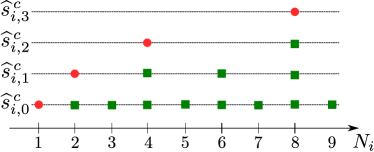
Figure 3: Illustration of the functioning of EFF-FEWA. The red circles denotes the number of pulls of arm $i$ at which a new estimate $\widehat{s}^{\,c}_{i,j}$ is created corresponding to a window $h=2^{j}$, while the green boxes indicate the number of pulls for which $\widehat{s}_{i,j}^{c}$ is updated with the last $2^{j}$ samples.

In Algorithm 3, we present EFF-FEWA, an algorithm that stores at most $2K\log_{2}(t)$ statistics. More precisely, for $j\leq\log_{2}(N_{i,t}^{\pi_{\rm EF}})$, we let $\widehat{s}_{i,j}^{\,p}$ and $\widehat{s}_{i,j}^{\,c}$ be the current and pending $j$-th statistic for arm $i$.

Algorithm 3 EFF-FEWA

0:  $\mathcal{K}$, $\delta_{0}$, $\alpha$

1:  pull each arm once, collect reward, and initialize $N_{i,K}\leftarrow 1$

2:  for $t\leftarrow K+1,K+2,\dots$ do

3:     $\delta_{t}\leftarrow\delta_{0}/(t^{\alpha})$

4:     $j\leftarrow 0$ {initialize bandwidth}

5:     $\mathcal{K}_{1}\leftarrow\mathcal{K}$ {initialize with all the arms}

6:     $i(t)\leftarrow{\tt none}$

7:     while $i(t)$ is ${\tt none}$ do

8:        $\mathcal{K}_{2^{j+1}}\leftarrow{{\textsc{EFF\_Filter}}}(\mathcal{K}_{2^{j}},j,\delta_{t})$

9:        $j\leftarrow j+1$

10:        if $\exists i\in\mathcal{K}_{2^{j}}$ such that $N_{i,t}\leq 2^{j}$ then

11:           $i(t)\leftarrow i$

12:        end if

13:     end while

14:     receive $r_{i}(N_{i,t+1})\leftarrow r_{i(t),t}$

15:     ${{\textsc{EFF\_Update}}}\mathopen{}\mathclose{{}\left(i(t),r_{i}(N_{i,t+1}),t+1}\right)$

16:  end for

As $N_{i,t}$ increases, new statistics $\widehat{s}_{i,j}^{\,c}$ for larger windows are created as illustrated in Figure 3. First, at any time $t$, $\widehat{s}_{i,j}^{\,c}$ is the average of $2^{j-1}$ consecutive reward samples for arm $i$ within the last $2^{j}-1$ sample. These statistics are used in the filtering process as they are representative of exactly $2^{j-1}$ recent samples. Second, $\widehat{s}_{i,j}^{\,p}$ stores the pending samples that are not yet taken into account by $\widehat{s}_{i,j}^{\,c}$. Therefore, each time we pull arm $i$, we update all the pending averages. When the pending statistic is the average of the $2^{j-1}$ last samples then we set $\widehat{s}_{i,j}^{\,c}\leftarrow\widehat{s}_{i,j}^{\,p}$ and reinitialize $\widehat{s}_{i,j}^{\,p}\leftarrow 0$.

Algorithm 4 EFF_Filter

0:  $\mathcal{K}_{2^{j}}$, $j$, $\delta_{t}$, $\sigma$

1:  $c(2^{j},\delta_{t})\leftarrow\sqrt{2\sigma^{2}/2^{j}\log{\delta^{-1}_{t}}}$

2:  $\widehat{s}_{\max,j}^{\,c}\leftarrow\max_{i\in\mathcal{K}_{h}}\widehat{s}_{i,j}^{\,c}$

3:  for $i\in\mathcal{K}_{h}$ do

4:     $\Delta_{i}\leftarrow\widehat{s}_{\max,j}^{\,c}-\widehat{s}_{i,j}^{\,c}$

5:     if $\Delta_{i}\leq 2c(2^{j},\delta_{t})$ then

6:        add $i$ to $\mathcal{K}_{2^{j+1}}$

7:     end if

8:  end for

8:  $\mathcal{K}_{2^{j+1}}$

Algorithm 5 EFF_Update

0:  $i$, $r$, $t$

1:  $N_{i(t),t}\leftarrow N_{i(t),t-1}+1$

2:  $R^{\rm total}_{i}\leftarrow R^{\rm total}_{i}+r$ {keep track of total reward}

3:  if $\exists j$ such that $N_{i,t}=2^{j}$ then

4:     $\widehat{s}_{i,j}^{\,c}\leftarrow R_{i}^{\rm total}/N_{i,t}$ {initialize new statistics}

5:     $\widehat{s}_{i,j}^{\,p}\leftarrow 0$

6:     $n_{i,j}\leftarrow 0$

7:  end if

8:  for $j\leftarrow 0\dots\log_{2}(N_{i,t})$ do

9:     $n_{i,j}\leftarrow n_{i}+1$

10:     $\widehat{s}_{i,j}^{\,p}\leftarrow\widehat{s}_{i,j}^{\,p}+r$

11:     if $n_{i,j}=2^{j}$ then

12:        $\widehat{s}_{i,j}^{\,c}\leftarrow\widehat{s}_{i,j}^{\,p}/2^{j}$

13:        $n_{i,j}\leftarrow 0$

14:        $\widehat{s}_{i,j}^{\,p}\leftarrow 0$

15:     end if

16:  end for

In analyzing the performance of EFF-FEWA, we have to account for two different effects: (1) the loss in resolution due to windows of size that increases exponentially instead of a fixed increment of 1, and (2) the delay in updating the statistics $\widehat{s}_{i,j}^{\,c}$, which do not include the most recent samples. We let $\overline{\mu}_{i}^{h^{\prime},h^{\prime\prime}}$ be the average of the samples between the $h^{\prime}$-th to last one and the $h^{\prime\prime}$-th to last one (included) with $h^{\prime\prime}>h^{\prime}$. FEWA was controlling $\overline{\mu}_{i}^{1,h}$ for each arm, EFF-FEWA controls $\overline{\mu}_{i}^{h^{\prime}_{i},h^{\prime}_{i}+2^{j-1}}$ with different $h^{\prime}_{i}\leq 2^{j-1}-1$ for each arm depending on when $\widehat{s}_{i,j}^{\,c}$ was refreshed last time. However, since the means of arms are non-increasing, we can consider the worst case when the arm with the highest mean available at that round is estimated with its last samples (the smaller ones) and the bad arms are estimated on their oldest possibles samples (the larger ones).

Lemma 6.

On favorable event $\xi_{t}$, if an arm $i$ passes through a filter of window $h$ at round $t$, the average of its $h$ last pulls cannot deviate significantly from the best available arm $i^{\star}_{t}$ at that round,

$$\overline{\mu}_{i}^{2^{j-1},2^{j}-1}\geq\mu^{+}_{t}(\pi_{\rm F})-4c(h,\delta_{t}).$$

We proceed with modifying Corollary 1 to have the following efficient version.

Corollary 4.

Let $i\in\textsc{op}$ be an arm overpulled by EFF-FEWA at round $t$ and $h_{i,t}^{\pi_{\rm EF}}\triangleq N_{i,t}^{\pi_{\rm EF}}-N_{i,t}^{\star}\geq 1$ be the difference in the number of pulls w.r.t. the optimal policy $\pi^{\star}$ at round $t$. On favorable event $\xi_{t}$, we have that

$$\mu^{+}_{t}(\pi_{\rm EF})-\overline{\mu}^{h_{i,t}^{\pi_{\rm EF}}}(N_{i,t})\leq\frac{4\sqrt{2}}{\sqrt{2}-1}c(h_{i,t}^{\pi_{\rm EF}},\delta_{t}).$$

Proof.

If $i$ was pulled at round $t$, then by the condition at Line 10 of Algorithm 3, it means that $i$ passes through all the filters until at least window $2^{f}$ such that $2^{f}\leq h_{i,t}^{\pi_{\rm EF}}<2^{f+1}$. Note that for $h_{i,t}^{\pi_{\rm EF}}=1$, then EFF-FEWA has the same guarantee as FEWA since the first filter is always up to date. Then for $h_{i,t}^{\pi_{\rm EF}}\geq 2,$

$$\overline{\mu}^{1,h_{i,t}^{\pi_{\rm EF}}}_{i}(N_{i,t}) \geq\overline{\mu}^{1,2^{f}-1}_{i}(N_{i,t})=\frac{\sum_{j=1}^{f}2^{j-1}\overline{\mu}_{i}^{2^{j-1},2^{j}-1}}{2^{f}-1}$$ (25)

$$\geq\mu^{+}_{t}(\pi_{\rm EF})-\frac{4\sum_{j=1}^{f}2^{j-1}c(2^{j-1},\delta)}{2^{f}-1}=\mu^{+}_{t}(\pi_{\rm EF})-4c(1,\delta_{t})\frac{\sum_{j=1}^{f}\sqrt{2}^{j-1}}{2^{f}-1}$$ (26)

$$=\mu^{+}_{t}(\pi_{\rm EF})-4c(1,\delta_{t})\frac{\sqrt{2}^{f}-1}{(2^{f}-1)(\sqrt{2}-1)}\geq\mu^{+}_{t}(\pi_{\rm EF})-4c(1,\delta_{t})\frac{1}{\sqrt{2}^{f}(\sqrt{2}-1)}$$ (27)

$$=\mu^{+}_{t}(\pi_{\rm EF})-\frac{4\sqrt{2}}{\sqrt{2}-1}c\mathopen{}\mathclose{{}\left(2^{f+1},\delta_{t}}\right)\geq\mu^{+}_{t}(\pi_{\rm EF})-\frac{4\sqrt{2}}{\sqrt{2}-1}c\mathopen{}\mathclose{{}\left(h_{i,t}^{\pi_{\rm EF}},\delta_{t}}\right),$$ (28)

where Equation 25 uses that the average of older means is larger than average of the more recent ones and then decomposes $2^{f}-1$ means onto a geometric grid. Then, Equation 26 uses Lemma 6 and makes the dependence of $c(2^{j-1},\delta)$ on $j$ explicit. Next, Equations 27 and 28 use standard algebra to get a lower bound and that $c(h,\delta)$ decreases with $h$. ∎

Using the result above, we follow the same proof as the one for FEWA and derive minimax and problem-dependent upper bounds for EFF-FEWA using Corollary 4 instead of Corollary 1.

Corollary 5 (minimax guarantee for EFF-FEWA).

For any rotting bandit scenario with means $\{\mu_{i}(n)\}_{i,n}$ satisfying Assumption 1 with bounded decay $L$ and any time horizon $T$, EFF-FEWA with $\delta_{t}=1/(t^{5})$, $\alpha=5$, and $\delta_{0}=1$ has its expected regret upper-bounded as

$$\mathbb{E}\mathopen{}\mathclose{{}\left[R_{{\color[rgb]{0.25,0.0,0.6}T}}\mathopen{}\mathclose{{}\left(\pi_{\rm EF}}\right)}\right]\leq 13\sigma\mathopen{}\mathclose{{}\left(\frac{\sqrt{2}}{\sqrt{2}-1}\sqrt{KT}+K}\right)\sqrt{\log(T)}+KL.$$

Corollary 6 (problem-dependent guarantee for EFF-FEWA).

For $\delta_{t}=1/(t^{5})$, the regret of EFF-FEWA is upper-bounded as

$$R_{T}(\pi_{\rm EF})\leq\sum_{i\in\mathcal{K}}\mathopen{}\mathclose{{}\left(\frac{C_{5}\frac{2}{3-2\sqrt{2}}\log(T)}{\Delta_{i,h_{i,T}^{+}-1}}+\sqrt{C_{5}\log(T)}+L}\right)\mathbin{\raisebox{2.15277pt}{,}}$$

with $C_{\alpha}\triangleq 32\alpha\sigma^{2}$ and $h_{i,T}^{+}$ defined in Equation 10.

Appendix F Numerical simulations: Stochastic bandits

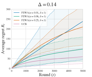
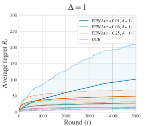
Figure 4: Comparing UCB1 and FEWA with $\Delta=0.14$ and $\Delta=1$.

In Figure 4 we compare the performance of FEWA against UCB (Lai and Robbins, 1985) on two-arm bandits with different gaps. These experiments confirm the theoretical findings of Theorem 1 and Corollary 2: FEWA has comparable performance with UCB. In particular, both algorithms have a logarithmic asymptotic behavior and for $\alpha=0.06$, the ratio between the regret of two algorithms is empirically lower than $2$. Notice, the theoretical factor between the two upper bounds is $80$ (for $\alpha=5$). This shows the ability of FEWA to be competitive for stochastic bandits.

References

- Audibert and Bubeck (2009) Jean-Yves Audibert and Sébastien Bubeck. Minimax policies for adversarial and stochastic bandits. In Conference on Learning Theory, 2009.
- Auer et al. (2002a) Peter Auer, Nicolò Cesa-Bianchi, and Paul Fischer. Finite-time analysis of the multiarmed bandit problem. Machine Learning, 47(2-3):235–256, 2002a.
- Auer et al. (2002b) Peter Auer, Nicolò Cesa-Bianchi, Yoav Freund, and Robert E. Schapire. The nonstochastic multi-armed bandit problem. Journal on Computing, 32(1):48–77, 2002b.
- Besbes et al. (2014) Omar Besbes, Yonatan Gur, and Assaf Zeevi. Stochastic multi-armed bandit problem with non-stationary rewards. In Neural Information Processing Systems, 2014.
- Besson (2018) Lilian Besson. SMPyBandits: An open-source research framework for single and multi-players multi-arm bandit algorithms in Python. Available at github.com/SMPyBandits/SMPyBandits, 2018.
- Bifet and Gavaldà (2007) Albert Bifet and Ricard Gavaldà. Learning from time-changing data with adaptive windowing. In International Conference on Data Mining, 2007.
- Bouneffouf and Féraud (2016) Djallel Bouneffouf and Raphael Féraud. Multi-armed bandit problem with known trend. Neurocomputing, 205(C):16–21, 2016.
- Bubeck and Cesa-Bianchi (2012) Sébastien Bubeck and Nicolò Cesa-Bianchi. Regret analysis of stochastic and nonstochastic multi-armed bandit problems. Foundations and Trends in Machine Learning, 5:1–122, 2012.
- Garivier and Moulines (2011) Aurélien Garivier and Eric Moulines. On upper-confidence-bound policies for switching bandit problems. In Algorithmic Learning Theory, 2011.
- Heidari et al. (2016) Hoda Heidari, Michael Kearns, and Aaron Roth. Tight policy regret bounds for improving and decaying bandits. In International Conference on Artificial Intelligence and Statistics, 2016.
- Lai and Robbins (1985) Tze L. Lai and Herbert Robbins. Asymptotically efficient adaptive allocation rules. Advances in Applied Mathematics, 6(1):4–22, 1985.
- Lattimore and Szepesvári (2020) Tor Lattimore and Csaba Szepesvári. Bandit algorithms. 2020.
- Levine et al. (2017) Nir Levine, Koby Crammer, and Shie Mannor. Rotting bandits. In Neural Information Processing Systems, 2017.
- Thompson (1933) William R. Thompson. On the likelihood that one unknown probability exceeds another in view of the evidence of two samples. Biometrika, 25:285–294, 1933.
- Warlop et al. (2018) Romain Warlop, Alessandro Lazaric, and Jérémie Mary. Fighting boredom in recommender systems with linear reinforcement learning. In Neural Information Processing Systems, 2018.