Lévy noise induced escape in the Morris-Lecar model

Abstract

The phenomenon of an excitable system producing a pulse under external or internal stimulation may be interpreted as a stochastic escape problem. This work addresses this issue by examining the Morris-Lecar neural model driven by symmetric $\alpha$-stable Lévy motion (non-Gaussian noise) as well as Brownian motion (Gaussian noise). Two deterministic quantities: the first escape probability and the mean first exit time, are adopted to analyse the state transition from the resting state to the excited state and the stability of this stochastic model. Additionally, a recent geometric concept, the stochastic basin of attraction is used to explore the basin stability of the escape region. Our main results include: (i) the larger Lévy motion index with smaller jump magnitude and the relatively small noise intensity are conducive for the Morris-Lecar model to produce pulses; (ii) a smaller noise intensity and a larger Lévy motion index make the mean first exit time longer, which means the stability of the resting state can be enhanced in this case; (iii) the effect of ion channel noise is more pronounced on the stochastic Morris-Lecar model than the current noise. This work provides some numerical simulations about the impact of non-Gaussian, heavy-tailed, burst-like fluctuations on excitable systems such as the Morris-Lecar system.

Keywords:

Lévy motion; Morris-Lecar model; First escape probability; Mean first exit time; Nonlocal partial differential equations.

1 Introduction

In recent years, there has been an increasing interest in the effects of noise in neuroscience. Because of the noisy environment that neurons live in, there are many sources of noise in the neuronal systems. These noisy sources include, for instance, random attacks caused by spontaneous release of neurotransmitters, synaptic noise from spontaneous postsynaptic potentials, small fluctuations in the electrical potential across the nerve-cell membrane, and the opening and closing of ion channels. Noise may induce various phenomena, such as oscillations [1, 2], chaos-like behaviors [3], state transitions [4], stochastic resonance [5, 6, 7], and spatial coherence resonance [8, 9, 10].

In this paper, we study the Morris-Lecar (ML) neuron model under the disturbance of (non-Gaussian) Lévy noise as well as (Gaussian) Brownian noise. As a simplified version of the Hodgkin-Huxley (HH) system, the ML model was first introduced to account for the electrical activities of the giant barnacle muscle fibers in invertebrates [11]. Since then, it becomes a canonical neuronal model because it can display two different forms of neuronal excitability behaviors under various parameter regimes. One form of excitability is not sensitive to external stimulation intensity, the discharge starting frequency can be very low, and the discharge range is relatively wide. This is called type I excitability. The type II excitability is relatively insensitive to external stimulation, and the discharge frequency is in a certain range. Meanwhile, from the point of view of bifurcation, type I excitability results from a saddle-node (tangent) bifurcation of equilibrium points on an invariant circle in ML model, while type II excitability corresponds to a subcritical Hopf bifurcation. The ML model is widely used in the theoretical research of the excitatory nerve discharge [12, 13, 14, 15, 16, 17]. Moreover, it can be used in cardiac cell modeling [18, 19]. As we known, $Na^{+}$ ions and $K^{+}$ ions cross the ion channels on the cell membrane back and forth, forming a transmembrane current and leading to the generation of an action potential or a spike - an abrupt and transient change of membrane voltage. An excitable system may be sensitive to noise [20]. So an excitable membrane can generate action potential when stimulated by a strong enough input or disturbed by noise.

Recent works on the stochastic ML model are mostly concerned with the model under Gaussian noise [21, 22, 23, 24, 25, 26]. In order to understand the information coding in the nervous systems, the influence of additive stochastic perturbation on bifurcation scenarios and the stationary distribution of stochastic ML system were studied in [27] based on random dynamical systems theory. The Gaussian noise induced multiple spatial coherence resonance and spatial patterns in excitable systems were revealed in [23, 24]. The methods based on asymptotic approximations of the stationary density function and most probable path were developed to understand the role of channel noise in spontaneous excitability [28]. However, Gaussian noise can not describe some fluctuations with bursts or intermittence or with heavy-tailed distributions, which are characteristics of $\alpha$-stable Lévy motions. Indeed, many complex phenomena involve fluctuations of the Lévy type, such as asset prices [29], turbulent motions of rotating annular fluid flows [30], a class of biological evolution [31], and random search [32]. Moreover, recent empirical research has shown that the probability distribution of anomalous (high amplitude) neural oscillations has heavier tail than the standard normal distribution [33]. The neuron systems with Lévy noise have attracted some recent attention [34, 35, 36, 37]. In fact, Lévy noise appears to be more reasonable than Gaussian noise, due to jumps by excitatory and inhibitory impulses caused by external disturbances in biological systems.

In this paper, we will consider the escape problem of the ML model with type II excitability under Lévy fluctuations. In this case the undisturbed system has unique equilibrium state. More concretely, we will study whether the system trajectory starting from the stable equilibrium point in the ML system reaches other region through a boundary under the influence of $\alpha$-stable Lévy noise. Two different deterministic quantities : the first escape probability (FEP) and the mean first exit time (MFET), are applied to analyse the problem. In order to quantify the escape behaviors, we should choose a proper escape region that contains the equilibrium point and a corresponding target region. The FEP is the likelihood for a system trajectory escaping to the target region, while MFET is the expected time for a system trajectory exiting the escape region. It turns out that both deterministic quantities are described by nonlocal partial differential equations (details in Sections 3 and 4). Then we will numerically calculate FEP of the solution stating from the escape region to the target region, and MFET of the solution stating from the escape region to the various outside regions.

The organization of the paper is as follows. In the next section we introduce the undisturbed ML model and the stochastic ML model driven by $\alpha$-stable Lévy noise. We also briefly review the $\alpha$-stable Lévy motion and two deterministic quantities: FEP and MFET, together with appropriate regions for computing these quantities. In Sections 3 and 4, we report numerical experiments on the effects of Lévy motion as well as Brownian motion in ML system, quantified by FEP and by MFET, respectively. Finally, we end the paper with a summary in Section 5.

2 The Morris-Lecar model

We now recall the undisturbed Morris-Lecar (ML) model and its disturbed version.

2.1 The undisturbed Morris-Lecar model

The deterministic Morris-Lecar (ML) model has been derived to describe giant barnacle (Balanus Nubilus) muscle fibres [27, 38], and it is represented by the following two-dimensional system:

$$\begin{split}C\frac{d{v_{t}}}{dt}&=-g_{Ca}m_{\infty}(v_{t})(v_{t}-V_{Ca})-g_{K}w_{t}(v_{t}-V_{K})-g_{L}(v_{t}-V_{L})+I,\\ \frac{d{w_{t}}}{dt}&=\varphi\frac{w_{\infty}(v_{t})-w_{t}}{\tau_{w}(v_{t})},\end{split}$$ (2.1)

where

$$m_{\infty}(v) =0.5[1+\tanh(\frac{v-V_{1}}{V_{2}})],$$

$$w_{\infty}(v) =0.5[1+\tanh(\frac{v-V_{3}}{V_{4}})],$$

$$\tau_{w}(v) =[\cosh(\frac{v-V_{3}}{2V_{4}})]^{-1}.$$

The variables $v_{t}$ and $w_{t}$ represent the membrane potential and the activation variable for the $K^{+}$ current, respectively. The parameter $C$ stands for the membrane capacitance. The first three terms in the right-hand side of the first equation in the system (2.1) respectively represent the voltage-gated $Ca^{2+}$ current, the voltage-gated delayed rectifier $K^{+}$ current and the leak current. The parameters $g_{Ca}$, $g_{K}$ and $g_{L}$ are the maximal conductance of the calcium current, potassium current and leak current, respectively. The parameters $V_{Ca}$, $V_{K}$ and $V_{L}$ are the reversal potentials of the calcium current, potassium current and leak current, respectively. Input current is represented by $I$. The constant $\varphi$ indicates the change between fast and slow scales of the model. Finally $V_{1},~{}V_{2},~{}V_{3},~{}V_{4}$ are tuning parameters for steady state and time constant.

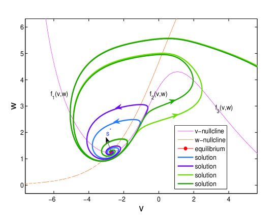
Figure 1: The phase portrait of the membrane potential $v_{t}$ and activation variable $w_{t}$ in the deterministic Morris-Lecar system (2.1) with type II excitability parameters and $I=88~{}(\mu A/cm^{2})$.

The parameter values for the type II excitability of ML model are [39, 40]: $C=20~{}\mu F/cm^{2}$, $V_{Ca}=120~{}mV$, $V_{K}=-84~{}mV$, $V_{L}=-60~{}mV$, $g_{Ca}=4.4~{}\mu S/cm^{2}$, $g_{K}=8~{}\mu S/cm^{2}$, $g_{L}=2~{}\mu S/cm^{2}$, $V_{1}=-1.2~{}mV$, $V_{2}=18~{}mV$, $V_{3}=2~{}mV$, $V_{4}=30~{}mV$ and $\varphi=0.04$. In this case the system possesses a unique equilibrium state for all values of $I$. This equilibrium is stable for $I<I_{H}\simeq 93.86~{}\mu A/cm^{2}$, and unstable beyond $I_{H}$ [27, 41]. In this study, we choose $I=88~{}\mu A/cm^{2}$, so the equilibrium state is stable. Furthermore, the resting cells at $I=88$ have excitability. Figure 1 shows the phase portrait of system (2.1), in which the $v$-nullcline is divided into three branches, the left branch $f_{1}$, the middle branch $f_{2}$ and the right branch $f_{3}$. Moreover, the resting potential corresponding to the equilibrium $s^{*}$ is located at the left branch $f_{1}$.

2.2 The stochastic Morris-Lecar model

We consider the Morris-Lecar model driven by symmetric $\alpha$-stable Lévy motion. This stochastic model is described by the following stochastic differential equations:

$$\begin{split}&d{v_{t}}=\frac{1}{C}[-g_{Ca}m_{\infty}(v_{t})(v_{t}-V_{Ca})-g_{K}w_{t}(v_{t}-V_{K})-g_{L}(v_{t}-V_{L})+I]dt+\sigma_{1}dL_{t}^{1},\\ &d{w_{t}}=\varphi\frac{w_{\infty}(x_{t})-w_{t}}{\tau_{w}(v_{t})}dt+\sigma_{2}dL_{t}^{2},\end{split}$$ (2.2)

where $L_{t}^{1}$ and $L_{t}^{2}$ are independent scalar symmetric $\alpha$-stable Lévy motions which have the same jump measure $\nu_{\alpha}$. The symbols $\sigma_{1},\sigma_{2}$ represent the noise intensities of the $L_{t}^{1}$ and $L_{t}^{2}$, respectively. As a special class of non-Gaussian process with jumps [42, 43], the $\alpha$-stable Lévy motion is defined by stable Lévy random variables. The distribution for a stable random variable is denoted as $S_{\alpha}(\delta,\beta,\gamma)$. Here $\alpha\in(0,2)$ is called the Lévy motion index (non-Gaussianity index), $\delta$ is the scale parameter, $\beta$ is the skewness parameter, and $\gamma$ is the shift parameter. Let us recall the definition of a symmetric $\alpha$-stable Lévy motion.

A symmetric $\alpha$-stable Lévy motion $L_{t}^{\alpha}$, with $0<\alpha<2$, is a stochastic process with the following properties [44, 45]:

(i) $L_{0}^{\alpha}$ = 0, almost surely (a.s);

(ii) $L_{t}^{\alpha}$ has independent increments;

(iii) $L_{t}^{\alpha}-L_{s}^{\alpha}\sim S_{\alpha}((t-s)^{\frac{1}{\alpha}},0,0)$;

(iv) $L_{t}^{\alpha}$ has stochastically continuous sample paths: for every $s$, $L_{t}^{\alpha}\to L_{s}^{\alpha}$ in probability, as $t\to s$.

The well-known Brownian motion $B_{t}$ corresponds to $\alpha$ being $2$. Moreover, a symmetric $\alpha$-stable Lévy motion can be represented as the triplet (0, 0, $\nu_{\alpha}$), where the jump measure $\nu_{\alpha}$ is defined as [42, 46]

$$\nu_{\alpha}=\frac{C_{\alpha}dy}{|y|^{1+\alpha}},$$ (2.3)

with

$$C_{\alpha}=\frac{\alpha}{2^{1-\alpha}\pi}\frac{\Gamma(1+\frac{\alpha}{2})}{\Gamma(1-\frac{\alpha}{2})}.$$ (2.4)

For $0<\alpha<2$, the following tail estimate of stable Lévy random variable $L$ holds [46]

$$\lim_{y\rightarrow\infty}y^{\alpha}\mathbb{P}(L>y)=C_{\alpha}\frac{1+\beta}{2}\sigma^{\alpha}.$$ (2.5)

This estimate indicates that the stable Lévy random variable $L$ has a “heavy tail”, which decays polynomially, unlike the tail estimate of Gaussian random variable, which decays exponentially.

In this paper, we make scale transformation of variables for the convenience of calculation. After this transformation, the stable equilibrium is $s^{*}=(-2.7277,1.2436)$ in the deterministic case (see equation (2.1)). The noise term $L_{t}^{1}$ represents current fluctuations in the environment and the noise term $L_{t}^{2}$ is understood as ion channel noise due to the opening and closing of ion channels. Indeed, there exists small fluctuations, always combined with unpredictable jumps of random environments in the biology growth process. Lévy motion $L_{t}^{\alpha}$ is suitable for simulating this type of noise. Moreover, $\alpha$-stable Lévy motion has larger jumps with lower jump frequencies when $\alpha$ closes to 0, while for $1<\alpha<2$, it has smaller jumps with higher jump probabilities. Especially, in the following numerical simulations, when $\alpha$ being 2, we respectively change the Lévy motion $L_{t}^{1}$, $L_{t}^{2}$ to independent Brownian motion $B_{t}^{1}$, $B_{t}^{2}$.

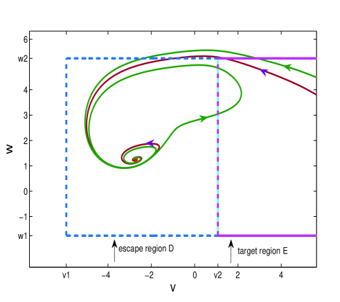
(a)

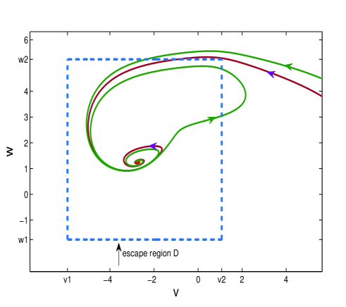
(b)

Figure 2: (a) The escape region we choose for FEP is $D:(-5.9277,1.0723)\times(-1.7564,5.2436)$ and target region is $E:[1.0723,\infty)\times[-1.7564,5.2436]$. (b) The escape region $D$ for MFET is the same as in (a), while the target region is $D^{c}$.

If ML system (2.1) is not subject to any disturbance, the stable equilibrium corresponds to the resting state of the ML system. When the system is under a perturbation, the solution orbit (or path) starting from the resting state may respond as a small oscillation near the resting state or produce a spike. This means that the ML system may have a state transition under the interference of noise. We further note that the $v$-nullcline is “cubic”, the middle branch $f_{2}$ in some sense separates the firing of an action potential from the subthreshold return to equilibrium [47]. If an orbit crosses the separatrix, it will be attracted by the right branch $f_{3}$ under the interference of non-Gaussian noise. Then we explain whether the orbit from the equilibrium state can be attracted by $f_{3}$ as an escape problem. Two deterministic quantities: FEP and MFET, are applied to this problem. In order to calculate FEP of the equilibrium $s^{*}$, the escape region $D$ (containing $s^{*}$) and the target region $E$ should be chosen. The two regions are $D:(-5.9277,1.0723)\times(-1.7564,5.2436)$ and $E:[1.0723,\infty)\times[-1.7564,5.2436]$ as shown in Figure 2. The FEP represents the probability of the solution orbit starting at a point in $D$ first escapes to region $E$. The reason we choose $\{(v,w)|v=1.0723,w\in R\}$ as a boundary line to calculate FEP is that $v>1.07234$ can be seen as the high electrical potential of a nerve cell. And if the solution orbit crosses this line $\{(v,w)|v=1.0723,w\in R\}$, it must be attracted by $f_{3}$. Meanwhile, the stability of the equilibrium under the stimulation by Lévy Motion and Brownain Motion will also be considered. We select region $D$ to compute MFET, which implies the mean first exit time of the solution orbit starting at a point in region $D$ escapes to region $D^{c}$.

3 First escape probability

The general form of the two-dimensional stochastic differential system (2.2) is as follows:

$$\begin{split}&d{v_{t}}=f_{1}(v_{t},w_{t})dt+\sigma_{1}dL_{t}^{1},\\ &d{w_{t}}=f_{2}(v_{t},w_{t})dt+\sigma_{2}dL_{t}^{2}.\end{split}$$ (3.1)

The infinitesimal generator $A$ of the system (3.1) is

$$Ap(v,w)= f_{1}(v,w)p_{v}(v,w)+f_{2}(v,w)p_{w}(v,w)$$

$$+\sigma_{1}^{\alpha}\int_{\mathbb{R}\setminus{\{0\}}}[p(v+v^{\prime},w)-p(v,w)]\nu_{\alpha}(dv^{\prime})$$

$$+\sigma_{2}^{\alpha}\int_{\mathbb{R}\setminus{\{0}\}}[p(v,w+w^{\prime})-p(v,w)]\nu_{\alpha}(dw^{\prime}).$$ (3.2)

When $L_{t}^{1},L_{t}^{2}$ are replaced by independent Brownian motions $B_{t}^{1},B_{t}^{2}$, the generator becomes

$$Ap(v,w)=f_{1}(v,w)p_{v}(v,w)+f_{2}(v,w))p_{w}(v,w)+\frac{\sigma_{1}^{2}}{2}p_{vv}(v,w)+\frac{\sigma_{2}^{2}}{2}p_{ww}(v,w).$$ (3.3)

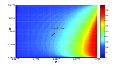
(a) $\alpha$ = 0.5, $\sigma$ = 0.5.

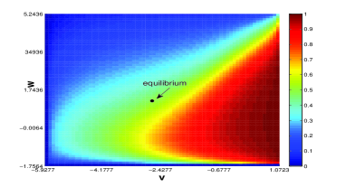
(e) $\alpha$ = 1.25, $\sigma$ = 0.25.

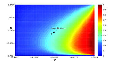
(b) $\alpha$ = 1, $\sigma$ = 0.5.

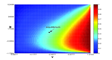
(f) $\alpha$ = 1.25, $\sigma$ = 0.5.

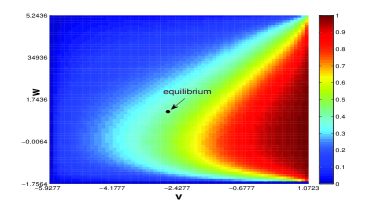
(c) $\alpha$ = 1.5, $\sigma$ = 0.5.

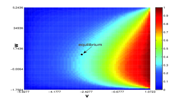
(g) $\alpha$ = 1.25, $\sigma$ = 0.75.

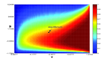
(d) Brownain case, $\sigma$ = 0.5.

(h) $\alpha$ = 1.25, $\sigma$ = 1.

Figure 3: FEP $p(v,w)$ from the escape region $D:(-5.9277,1.0723)\times(-1.7564,5.2436)$ to target region $E:[1.0723,\infty)\times[-1.7564,5.2436]$. The color map depends on Lévy motion index $\alpha$ and noise intensity $\sigma$ ($\sigma_{1}=\sigma_{2}=\sigma$). (a)-(d) Influence of Lévy motion index $\alpha$ on FEP for different values of $\alpha$ with fixed noise intensity $\sigma=0.5$. (e)-(h) Influence of noise intensity $\sigma$ on FEP for different values of $\sigma$ with fixed Lévy motion index $\alpha=1.25$. The color bar in all figures is set to the same scale, red making 1 and blue making 0.

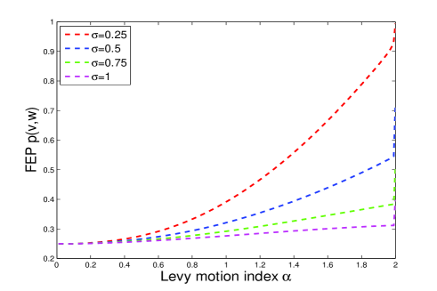
(a)

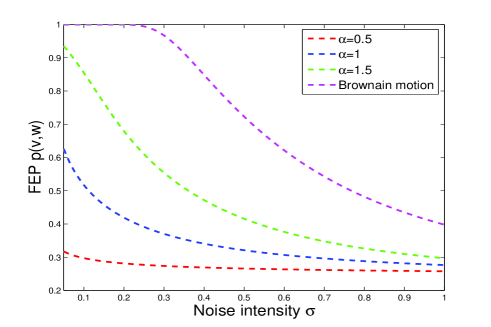
(b)

Figure 4: FEP $p(v,w)$ at the equilibrium $s^{*}=(-2.7277,1.2436)$, $\sigma_{1}=\sigma_{2}=\sigma$. (a) Effect of Lévy motion index $\alpha$ on FEP at $s^{*}$ for various values of noise intensity $\sigma$ (red: $\sigma$ = 0.25, blue: $\sigma$ = 0.5, green: $\sigma$ = 0.75, pink: $\sigma$ = 1). (b) Effect of noise intensity $\sigma$ on FEP at $s^{*}$ for various values of Lévy motion index $\alpha$ (red: $\alpha$ = 0.5, blue: $\alpha$ = 1, green: $\alpha$ = 1.5, pink: $\alpha$ being 2 indicates to case of Brownain motion).

The first escape probability (FEP) here is employed to characterize the likelihood of the escape from the low potential region to the high potential region for the ML system. It is denoted as $p(v,w)$, which is used to characterize the probability of the solution orbit starting at $(v,w)$ in a open region $D$ first escaping to a target region $E$. The escape probability $p(v,w)$ can be solved by the following integral-differential equation with a Balayage-Dirichlet exterior boundary condition [45]:

$$Ap(v,w)=0,\quad(v,w)\in D,$$

$$p(v,w)=\begin{cases}1,\quad(v,w)\in E,\\ 0,\quad(v,w)\in D^{c}\setminus{E}.\end{cases}$$ (3.4)

Here $D^{c}$ is the complement set of the bounded region $D$. Results about the existence and uniqueness of solutions to nonlocal systems similar to integral-differential equation (3) may be found in [48, 49, 50]. The equation (3) can be solved by an effective numerical scheme given in the Appendix.

Figure 3 shows the numerical simulation of the FEP for different Lévy motion index $\alpha$ and noise intensity $\sigma$ ($\sigma_{1}=\sigma_{2}=\sigma$). In Figure 3(a)-(d), the noise intensity $\sigma=0.5$, the area of high FEP (red region) gradually becomes bigger with the increase of $\alpha$. In Figure 3(e)-(h), when the Lévy motion index $\alpha=1.25$, the area of high FEP (red region) gradually becomes smaller with the increase of $\sigma$. From Figure 3(a)-(h), we conclude that the escape probability varies with initial membranae potential, in the following way: when the noise intensity is fixed ($\sigma=0.5$), the larger Lévy motion index $\alpha$, the more likely the low potential state of the ML system becomes excited. However, when the Lévy motion index $\alpha$ is fixed ($\alpha=1.25$), the smaller the noise intensity, the easier the ML system gets excited.

Figure 4 depicts the influence of Lévy motion index $\alpha$ and noise intensity $\sigma$ ($\sigma_{1}=\sigma_{2}=\sigma$) on FEP of the equilibrium $s^{*}$. In Figure 4(a), Lévy motion index $\alpha$ is from 0.01 to 1.99 and the step size is 0.01, the value of $\alpha$ being 2 corresponds to the Brownain Motion case. It can be seen that for fixed noise intensity $\sigma$, FEP increases as $\alpha$ increases, and grows rapidly at $\alpha$ being 2. This means that smaller jumps with higher frequencies are more beneficial to make the system from the resting state to the excited state and generate a pulse. In Figure 4(b), for various value of fixed $\alpha$ ($\alpha$ = 0.5, 1, 1.5, 2), the smaller noise intensity, the higher FEP, the easier the system gets into the excited state. When $\alpha=0.5$, FEP keeps almost unchanged as the noise intensity increases, which means that noise has less effect on the state transitions. When $\alpha=1$ and $\alpha=1.5$, FEP drops rapidly with small noise intensity and as the noise intensity increases, the trend of FEP tends to be steady. Finally, when $\alpha$ being 2, with increasing $\sigma$ from 0.05, FEP remains at 1 until $\sigma_{a}$ (=0.185), and then it becomes monotonously decreasing. This means when the system is affected by the Brownian motion, the solution path starting at the equilibrium point can definitely escape region $D$ for very small noise intensity. In general, the larger the Lévy motion index $\alpha$ and the smaller noise intensity $\sigma$, the more likely for the ML system to reach the excited state and generate a pulse. Compared with non-Gaussian Lévy noise, the Gaussian Brownian noise is easier to make the system transition from the resting state to the excited state.

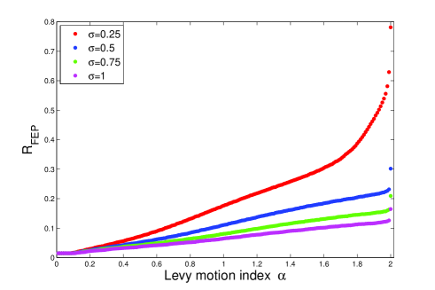
(a)

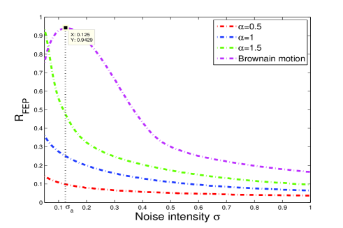
(b)

Figure 5: Effect of noise intensity and Lévy motion index on the $R_{FEP}$. The threshold $p^{*}$ to compute $R_{FEP}$ is chosen as 0.8. (a) $R_{FEP}$ against Lévy motion index $\alpha$ for various noise intensity $\sigma$ (red: $\sigma$ = 0.25, blue: $\sigma$ = 0.5, green: $\sigma$ = 0.75, pink: $\sigma$ = 1). (b) $R_{FEP}$ against noise intensity $\sigma$ for various Lévy motion index $\alpha$ (red: $\alpha$ = 0.5, blue: $\alpha$ = 1, green: $\alpha$ = 1.5, pink: $\alpha$ being 2 indicates to case of Brownain motion.

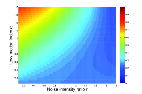
(a) $r=\sigma_{2}/\sigma_{1}$, fixed $\sigma_{1}=0.5$.

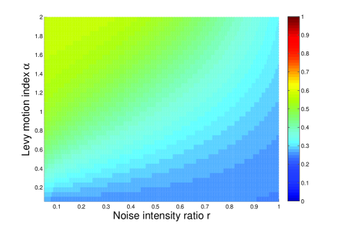
(b) $r=\sigma_{2}/\sigma_{1}$, fixed $\sigma_{1}=1$.

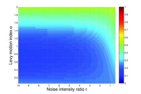
(c) $r=\sigma_{2}/\sigma_{1}$, fixed $\sigma_{2}=0.5$.

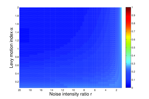
(d) $r=\sigma_{2}/\sigma_{1}$, fixed $\sigma_{2}=1$.

Figure 6: FEP $p(v,w)$ at the equilibrium $s^{*}$ = (-2.7277, 1.2436), the color map depends on noise intensity ratio $r$ and Lévy motion index $\alpha$. The color bar in all figures is set to the same scale, red making 1 and blue making 0. (a) Fixed $\sigma_{1}=0.5$, $\sigma_{2}\in[0.05,1]$. (b) Fixed $\sigma_{1}=1$, $\sigma_{2}\in[0.05,1]$. (c) $\sigma_{1}\in[0.05,1]$, fixed $\sigma_{2}=0.5$. (d)$\sigma_{1}\in[0.05,1]$, fixed $\sigma_{2}=1$.

Furthermore, inspired by [51] and [52], we would like to employ the stochastic basin of attraction (SBA) to quantify the basin stability in the escape region $D$. We denote the stochastic basin of the attractor $f_{3}$ in the region $D$ is the set $K(p^{*})=\{(v,w)\in D|p(v,w)>p^{*}\}$, where $p^{*}$ indicates a high probability level (‘threshold’). The set $K(p^{*})$ means the orbits starting from the points in the region $D$ reach to the region $E$ with high probability (we ignore the initial points whose solution have a ‘small’ probability away from by $f_{3}$). The basin stability in region $D$ can be quantified in terms of its area, that is, $S_{FEP}$ represents the area of $K(p^{*})$. More specifically, when the FEP of the solution orbit from the points in $D$ is greater than the threshold $p^{*}$, we record these points and then calculate the area of the region composed of these points as $S_{FEP}$. The normalized $S_{FEP}$ is [36]

$$R_{FEP}=\frac{S_{FEP}(p^{*})}{S_{D}},$$ (3.5)

where $S_{D}$ is the area of region $D$.

Now we choose $p^{*}=0.8$ to compute $R_{FEP}$ as illustrated in Figure 5. In Figure 5, we let the noise intensity $\sigma_{1}=\sigma_{2}=\sigma$. From Figure 5(a), we can see that for a fixed noise intensity, the larger Lévy motion index, the larger $R_{FEP}$. When $\alpha$ being 2 (corresponding to the case of Brownian motion), the four curves all get their maximum and present a rapid growth. The situation shows that compared with the effect of Lévy noise on the ML system, there are more orbits starting from the points in the low potential region to escape to the high potential region with high probability in the case of Brownian motion. It also indicates that Gaussian noise makes the ML system more accessible to the excited state. In Figure 5(b), as can be seen, $R_{FEP}$ decreases with the increase of $\sigma$ for fixed $\alpha$ besides $\alpha$ being 2. When $\alpha$ being 2, as the noise intensity $\sigma$ increases, $R_{FEP}$ increases monotonously, reaches its maximum at $\sigma_{b}$, and then decreases as $\sigma$ continues to grow. As a whole, the lager Lévy motion index and the smaller noise intensity are beneficial to more solution orbits with the point in region $D$ as the initial point escape to the target region $E$.

The pictorial representation of the aforementioned results gives us an inspiration for the stochastic escape problem, i.e., if we expect the ML system to escape from the resting state to the excited state, then a smaller noise intensity and a larger Lévy motion index $\alpha$ (smaller jump magnitude with higher frequency) should be selected.

Next, we denote a new parameter named noise intensity ratio

$$r=\sigma_{2}/\sigma_{1}.$$ (3.6)

In order to better understand the influence of noise intensity and Lévy motion index on FEP starting from the equilibrium point, we plot FEP depending on Lévy motion index $\alpha$ and noise intensity ratio $r$, as shown in Figure 6. In Figure 6(a)-(b), we fix separately $\sigma_{1}=0.5$ and $\sigma_{1}=1$, $\sigma_{2}$ belongs to interval $[0.05,1]$. It can be seen that the first escape probabilities all have lager value for larger Lévy motion index $\alpha$ and smaller noise intensity ratio $r$. And when $\sigma_{1}$ is fixed, the smaller $\sigma_{2}$ and the larger $\alpha$, the more likely the ML system is to generate spikes. While in Figure 6(c)-(d), we fix separately $\sigma_{2}=0.5$ and $\sigma_{2}=1$, $\sigma_{1}$ belongs to interval $[0.05,1]$. It can be seen that, for fixed noise intensity ratio $r$, FEP is larger for the lager Lévy motion index $\alpha$ in Figure 6(c), but FEP is smaller for lager $\alpha$ and smaller $\sigma_{1}$ (lager noise intensity ratio $r$) with fixed $\sigma_{2}=1$ in Figure 6(d). And when $\sigma_{2}$ is fixed, $\sigma_{1}$ has little effect on the state transition of the ML system. In general, we infer that the noise intensity $\sigma_{2}$ has a greater influence on escape probability for the same $\alpha$.

4 Mean first exit time

(a) $\alpha$ = 0.5, $\sigma$ = 0.75.

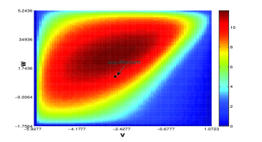
(e) $\alpha$ = 1.25, $\sigma$ = 0.25.

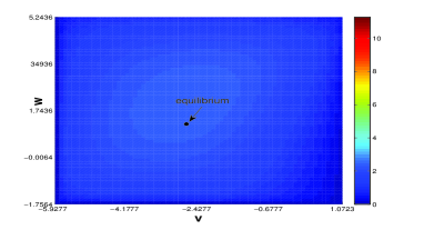
(b) $\alpha$ = 1, $\sigma$ = 0.75.

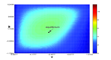
(f) $\alpha$ = 1.25, $\sigma$ = 0.5.

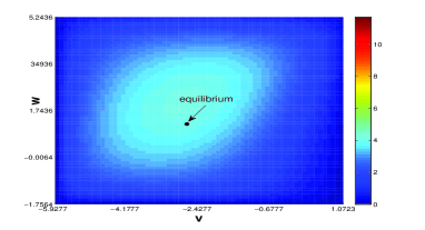
(c) $\alpha$ = 1.5, $\sigma$ = 0.75.

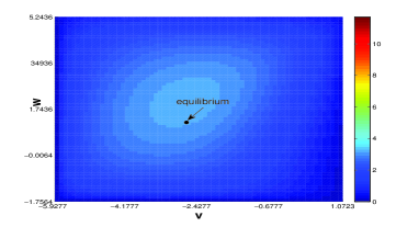
(g) $\alpha$ = 1.25, $\sigma$ = 0.75.

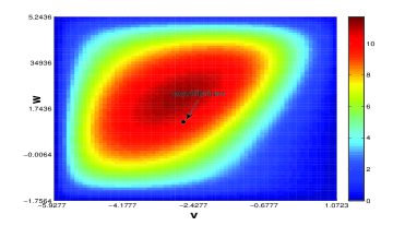
(d) Brownain case, $\sigma$ = 0.75.

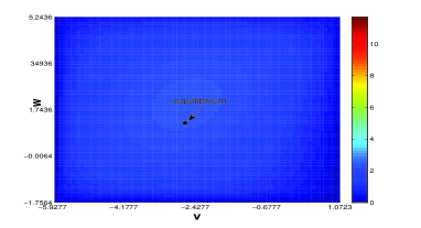
(h) $\alpha$ = 1.25, $\sigma$ = 1.

Figure 7: MFET $u(v,w)$ from the escape region $D:(-5.9277,1.0723)\times(-1.7564,5.2436)$ to the region $D^{c}$. The colour map depends on Lévy motion index $\alpha$ and noise intensity $\sigma$ ($\sigma_{1}=\sigma_{2}=\sigma$). (a)-(d) correspond to fixed noise intensity $\sigma=0.75$ and different Lévy motion index $\alpha=0.5,~{}1,~{}1.5,~{}2$. (e)-(h) correspond to fixed $\alpha=1.25$ and different $\sigma=0.25,~{}0.5,~{}0.75,~{}1$. All figures are unified into an identical color map with the same scale, red marking 11.7084 and blue making 0.

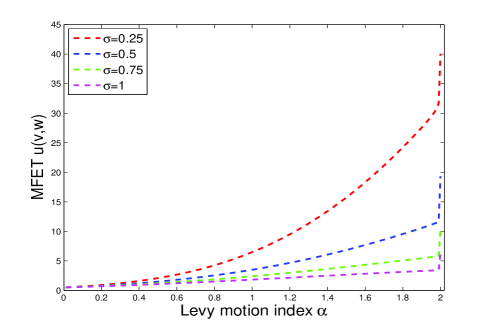
(a)

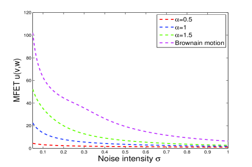
(b)

Figure 8: MFET $u(v,w)$ of the equilibrium $s^{*}$= (-2.7277, 1.2436). Here $\sigma_{1}=\sigma_{2}=\sigma$. (a) Effect of Lévy motion index $\alpha$ on MFET at $s^{*}$ with different noise intensity $\sigma$ (red: $\sigma$ = 0.25, blue: $\sigma$ = 0.5, green: $\sigma$ = 0.75, pink: $\sigma$ = 1). (b) Effect of noise intensity $\sigma$ on MFET at $s^{*}$ with different Lévy motion index $\alpha$ (red: $\alpha$ = 0.5, blue: $\alpha$ = 1, green: $\alpha$ = 1.5, pink: $\alpha$ being 2 indicates to case of Brownain motion).

In this section, we use another quantity: the mean first exit time to examine the effects of Lévy motion index and noise intensity on the behavior of the escape problem. Back to the general two-dimensional stochastic system (3.1) in the previous section. The first exit time for a solution orbit starting at $(v,w)$ in a region $D$ is defined as

$$\tau(\omega,(v,w))=\inf\{t\geq 0:(v_{0},w_{0})=(v,w),(v_{t},w_{t})\in D^{c}\},$$

where $D^{c}$ is the complement set of the bounded region $D$ in $\mathbb{R}^{2}$. The mean first exit time (MFET) is denoted as

$$u(v,w):=\mathbb{E}\tau(\omega,(v,w))\geq 0.$$

It is the ‘average’ residence time of a solution orbit initially at $(v,w)$ inside region $D$ before escaping to another region. The difference between a Gaussian and a non-Gaussian process is that the orbit typically hits the boundary of region $D$ for the Brownian motion case, while it may jumps outside of region $D$ for Lévy motion case. The MFET $u(v,w)$ satisfies the following nonlocal integral-differential equation with an exterior boundary condition [45]:

$$Au(v,w)=-1,\qquad (v,w)\in D,$$ (4.1)

$$u(v,w)=0,\qquad (v,w)\in D^{c}.$$

Here the generator $A$ is defined in equation (3). The existence and uniqueness of solution to the equation (4.1) satisfied by the mean first exit time of the stochastic ML system (2.2) can be proved according to the third section in [53] and Theorem 3.2 in [54]. The equation (4.1) can be solved by an effective numerical scheme given in the Appendix.

MFET can be used as a tool to measure the stability of a system: The longer the MFET, the more stable the resting state. For ML system, we choose the low potential region $D$ enclosing the resting state $s^{*}$ in phase plane to calculate the MFET. We plot MFET $u(v,w)$ from escape region $D:(-5.9277,1.0723)\times(-1.7564,5.2436)$ to the region $D^{c}$ as shown in Figure 7. In Figure 7(a)-(d), noise intensity $\sigma$ is fixed as $\sigma=0.75$, the MFET of non-exciting region gradually increases with the increase of Lévy motion index $\alpha$ ($\alpha$= 0.5, 1, 1.5, 2). In Figure 7(e)-(h), as $\sigma$ increases, the MFET of non-exciting region is getting less for fixed $\alpha=1.25$. In fact, the solution orbit starting at the equilibrium point will stay there forever without noise. Now for noisy situations, the solution orbits may stay in region $D$ for a finite time and then escape to another region. So we can employ the MFET to characterize the relative stability of the solution orbits starting at the points in region $D$. From Figure 7(a)-(h), we observe that larger Lévy motion index $\alpha$ and smaller noise intensity $\sigma$ are beneficial to the stability of the region $D$.

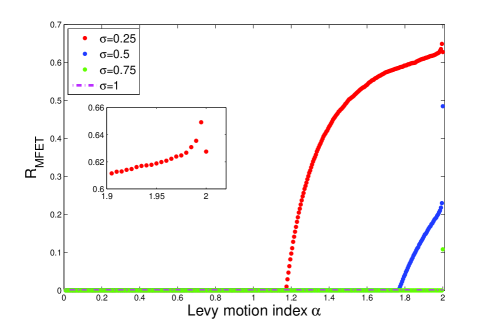
(a)

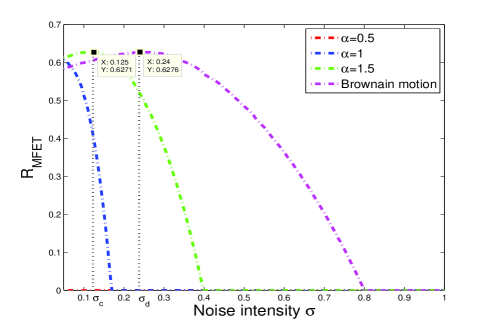
(b)

Figure 9: Effect of noise intensity $\sigma$ and Lévy motion index $\alpha$ on the $R_{MFET}$. The threshold $u^{*}$ to compute $R_{MFET}$ is chosen as 10. Here we choose $\sigma_{1}=\sigma_{2}=\sigma$. (a) $R_{MFET}$ against Lévy motion index $\alpha$ for various noise intensity $\sigma$ (red: $\sigma$ = 0.25, blue $\sigma$ = 0.5, green $\sigma$ = 0.75, pink $\sigma$ = 1). (b) $R_{MFET}$ against noise intensity $\sigma$ for various Lévy motion index $\alpha$ (red: $\alpha$ = 0.5, blue: $\alpha$ = 1, green: $\alpha$ = 1.5, pink: $\alpha$ indicates to case of Brownain motion).

Similarly, Figure 8 depicts the change of MFET for the resting state in some cases. In Figure 8, we denote the Lévy motion index $\alpha\in(0,2)$ (the case where $\alpha$ being 2 is replaced by the Brownian motion) and the noise intensity $\sigma\in(0,1]$ ($\sigma_{1}=\sigma_{2}=\sigma$). It can be seen from the Figure 8(a), the larger $\alpha$, the greater MFET, and this is more noticeable for smaller noise intensity. And when the noise intensity $\sigma$ is larger ($\sigma=1$), the Lévy motion $\alpha$ is less effect on the MFET for the resting state. No matter what the noise intensity is ($\sigma=0.25,~{}0.5,~{}0.75,~{}1$), MFET for the resting state reaches the maximum at $\alpha$ being 2. The MFET for the Brownian motion is longer than for the Lévy motion, which may be due to the fact that the trajectory of Brownian motion is continuous and cannot jump. This also indicates the resting state is more stable under Brownian motion than under Lévy motion.

Indeed, MFET is solution to the (4.1), with $A$ in (3) for Lévy case and (3.3) for Brownain case. In Figures 8(a), the numerical simulation indicates discontinuity as $\alpha$ approaching 2. Theoretically, although the characteristic function of Lévy motion $L_{t}^{\alpha}$ satisfies $e^{-t|\xi|^{\alpha}}\rightarrow e^{-t|\xi|^{2}}$ as $\alpha\rightarrow 2$, the MFET for Lévy case may not approach that for Brownian case as $\alpha\rightarrow 2$; see Theorem 2.2 in [55]. This remark also applies to FEP.

In addition, Figure 8(b) further depicts the effect of noise intensity $\sigma$ on MFET for the resting state with different Lévy motion index $\alpha$. As can be seen, MFET decreases with the increasing of $\sigma$ for fixed $\alpha$ and the change curve of MFET is not very obvious when $\alpha$ is small, such as $\alpha=0.5$. On the contrary, when $\alpha$ is lager, the change curve of MFET goes down very fast at first and tends to level off with the increasing of $\sigma$. The noise intensity has little effect on the MFET for fixed smaller Lévy motion index $\alpha$ ($\alpha=0.5$). In general, the smaller the noise intensity $\sigma$ and the larger the Lévy motion $\alpha$, the longer the time for the orbit to escape the region $D$. Therefore, if we expect the resting state to be more stable, then a smaller noise intensity $\sigma$ and a larger $\alpha$ (smaller jump magnitude with higher frequency) should be responsible.

We now define another stability concept via to the stochastic basin of attraction in Section 3. Let $M(u^{*})=\{(v,w)\in D|u(v,w)>u^{*}\}$, i.e., the solution orbit starting from region $D$ and remaining there for a finite time (remarked by a threshold $u^{*}$). Then we also quantify the basin stability in region $D$ based on its area [36]:

$$R_{MFET}=\frac{S_{MFET}(u^{*})}{S_{D}},$$ (4.2)

where $S_{MFET}$ is the area of $M(u^{*})$, and $S_{D}$ is the area of $D$. $R_{MFET}$ is the normalization of $S_{MFET}$.

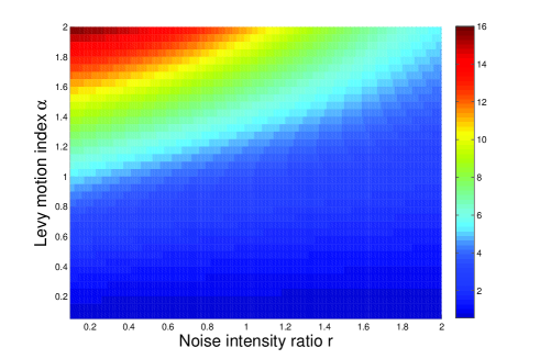
(a) $r=\sigma_{2}/\sigma_{1}$, fixed $\sigma_{1}=0.5$.

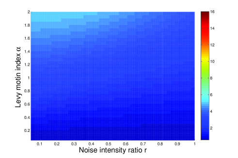
(b) $r=\sigma_{2}/\sigma_{1}$, fixed $\sigma_{1}=1$.

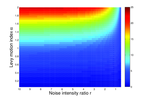
(c) $r=\sigma_{2}/\sigma_{1}$, fixed $\sigma_{2}=0.5$.

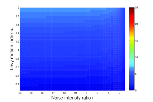
(d) $r=\sigma_{2}/\sigma_{1}$, fixed $\sigma_{2}=1$.

Figure 10: MFET $u(v,w)$ of the equilibrium $s^{*}$ = (-2.7277, 1.2436), the color graphs depend on noise intensity ratio $r$ and Lévy motion index $\alpha$. (a)-(b) $\sigma_{2}\in[0.05,1]$, fixed $\sigma_{1}=0.5,~{}1$, respectively. The color bar of (a) and (b) is taken the same scale. (c)-(d) $\sigma_{1}\in[0.05,1]$, fixed $\sigma_{2}=0.5,~{}1$, respectively. The color bar of (c) and (d) is taken the same scale.

In the following, as an example, we make $u^{*}=10$ to calculate the $R_{MFET}$, the results are shown in Figure 9. Figure 9(a) depicts $R_{MFET}$ against the Lévy motion index $\alpha$ for various values of $\sigma$ ($\sigma_{1}=\sigma_{2}=\sigma$). It can be seen that for fixed $\sigma=0.25$ and $\sigma=0.5$, the $R_{MFET}$ remains 0 in the beginning, then increases with increasing $\alpha$ besides $\alpha$ being 2 (corresponding to the case of Brownian motion). While for the other two curves of $R_{MFET}$ with $\sigma=0.75$ and $\sigma=1$, the $R_{MFET}=0$, which means that for higher noise intensity the solution orbit starting at a point in region $D$ gets out of region $D$ quickly. This also indicates the region $D$ is less stable under the higer noise intensity. Special cases occur when $\alpha$ being 2: for $\sigma=0.5$ and $\sigma=0.75$, the values of $R_{MFET}$ both have a jumping growth; for $\sigma=0.25$, $R_{MFET}$ suddenly decreases and the value of $R_{MFET}$ has no change for $\sigma=1$. Figure 9(b) depicts $R_{MFET}$ against noise intensity $\sigma$ for various values of $\alpha$. It shows that for $\alpha=1.5$ and $\alpha$ being 2, the curve of $R_{MFET}$ transits from increasing to decreasing at $\sigma_{c}$ and $\sigma_{d}$, respectively, then goes down to zero as further increasing $\sigma$. While when $\alpha=1$, $R_{MFET}$ gradually decreases from positive to zero, then keep zero with the further increase of $\sigma$. At the same time, $R_{MFET}=0$ when $\alpha=0.5$, which indicates that a solution orbit starting at $(v,w)\in D$ escapes quickly for smaller $\alpha$, that is, the region $D$ is less stable for the smaller Lévy motion index. Here we choose the initial value $\sigma=0.05$ and the same partition $\Delta\sigma=0.005$. Moreover, we can find that the curve with $\alpha=2$ and $\alpha=1.5$, $\alpha=1$ has a intersection point, respectively. For fixed noise intensity, larger $\alpha$ has smaller $R_{MFET}$ before the intersection point and it’s the opposite after the intersection point.

As in the section 3, we also plot MFET for the resting state depending on noise intensity ratio $r$ and Lévy motion index $\alpha$ as shown in the Figure 10. In Figure 10(a)-(b), we respectively fix $\sigma_{1}=0.5$ and $\sigma_{1}=1$ as well $\sigma_{2}$ belongs to interval $[0.05,1]$. It can be seen that MFET has lager value for lager Lévy motion index $\alpha$ and smaller noise intensity ratio $r$. Meanwhile, when fix $\alpha<1$, whether in Figure 10(a) or Figure 10(b), the noise intensity ratio $r$ has a small effect on MFET of the equilibrium point; and when fix $\alpha>1$, the change of MFET is obvious. This just verifies that the jump property of Lévy motion. While in Figure 10(c)-(d), we respectively fix $\sigma_{2}=0.5$ and $\sigma_{2}=1$ as well $\sigma_{1}$ belongs to interval $[0.05,1]$. We observe that the lager $\alpha$, the longer MFET and the noise intensity $\sigma_{1}$ has less effect on the system for the fxed $\sigma_{2}$ ($\sigma_{2}=1$). Comparing Figure 10(c) with Figure 10(d) , when fix $\alpha>1$, for the same $\sigma_{1}$ (the $r$ in (d) is 2 times that in (c)), the MFET with $\sigma_{2}=0.5$ obviously larger than the MFET with $\sigma_{2}=1$, which indicates the resting state is relatively stable for smaller $\sigma_{2}$. In general, the larger the Lévy motion index and the smaller the noise intensity, the more stable the system.

5 Conclusion

In summary, we focus on the escape problem driven by a symmetric $\alpha$-stable Lévy noise (non-Gaussian noise) in Morris-Lecar (ML) model. We have provided a method to quantify the dynamics of escape from the resting state of the system by means of two deterministic indices: the first escape probability (FEP) and the mean first exit time (MFET). To be specific, we have used the method to describe the state transition from the resting state to the excited state. To simulate the firing behavior of neurons and calculate FEP, we have chosen the appropriate escape region containing the equilibrium point and the target region. Meanwhile, we have depicted the stability of the escape region in terms of MFET.

Through numerical simulation and analysis, we have found that the noise intensities $\sigma_{1}$, $\sigma_{2}$ and the jump size of $\alpha$-stable Lévy motion have significant and delicate influences on the FEP and MFET. We have also discovered that for smaller jumps of the Lévy motion and relatively smaller noise intensity, FEP is larger, which means that they are conducive to the production of spikes. However, higher noise intensity and larger jumps of the Lévy motion shortens the MFET, which means the escape region is less stable for higher noise intensity and larger jumps of the Lévy motion. Moreover, the Brownian motion (Gaussian noise) has been also considered and compared with the Lévy motion case. Compared with Lévy motion, FEP is larger and MEFT is longer under the influence of Brownian motion. This means that the perturbed system is more likely to switch from the resting state to the excited state, and the resting state is relatively more stable in the Brownian case. Meanwhile, we have explored the stochastic basin of attraction for the stability of a region. By calculating the area of high FEP and long MFET for various Lévy motion index $\alpha$ and noise intensity $\sigma$, we have revealed that larger $\alpha$ and smaller noise intensity $\sigma$ are beneficial for the stability of the region $D$.

By calculating the impact of the noise intensity ratio $r$ and Lévy motion index $\alpha$ on FEP of the equilibrium point, we have revealed that $\sigma_{2}$ (intensity for ion channel noise) has more pronounced influence on the system than $\sigma_{1}$ (intensity for current fluctuations), for fixed Lévy motion index $\alpha$. To be specific, for the state transition probability of the system, ion channel noise has a greater impact than current noise. The smaller the $\sigma_{2}$ and the larger Lévy motion index $\alpha$, the more likely the stochastic ML system is to generate a pulse. For the MFET at the equilibrium point, larger Lévy motion index $\alpha$ and smaller noise intensities $\sigma_{1}$, $\sigma_{2}$, the more stable the resting state in the ML system.

We have applied the knowledge of stochastic dynamics to explore the phenomenon of noise-induced escape in a neural system. This work provides some mathematical understanding about the impact of non-Gaussian, heavy-tailed, burst-like fluctuations on excitable systems such as the Morris-Lecar system.

Appendix: Numerical simulation

We use an efficient numerical finite difference scheme [56] to compute the FEP (equation (3)) and MFET (equation (4.1)). This method is revised for our model in $(v,w)\in D=(a,b)\times(c,d)$, $E=[a^{\prime},b^{\prime}]\times[c,d]$ by a scalar conversion $v=\frac{b-a}{2}s+\frac{a+b}{2}$, and $w=\frac{d-c}{2}k+\frac{c+d}{2}$ for $s\in(-1,1),k\in(-1,1)$. If we let $m(s,k)=p(\frac{b-a}{2}s+\frac{a+b}{2},\frac{d-c}{2}k+\frac{c+d}{2})$, equation (3) is discretized as follows:

$$Ap(v,w)= \frac{2}{b-a}f_{1}(\frac{b-a}{2}s+\frac{a+b}{2},\frac{d-c}{2}k+\frac{c+d}{2})m_{s}$$

$$+\frac{2}{d-c}f_{2}(\frac{b-a}{2}s+\frac{a+b}{2},\frac{d-c}{2}k+\frac{c+d}{2})m_{k}$$

$$-\frac{\sigma_{1}^{\alpha}C_{\alpha}}{\alpha}(\frac{b-a}{2})^{\alpha}\left[\frac{1}{(1+s)^{\alpha}}+\frac{1}{(1-s)^{\alpha}}\right]m(s,k)$$

$$+\sigma_{1}^{\alpha}C_{\alpha}(\frac{b-a}{2})^{\alpha}\int_{-1-s}^{1-s}\frac{m(s+s^{\prime},k)-m(s,k)}{\mid s^{\prime}\mid^{1+\alpha}}ds^{\prime}$$

$$-\frac{\sigma_{2}^{\alpha}C_{\alpha}}{\alpha}(\frac{d-c}{2})^{\alpha}\left[\frac{1}{(1+k)^{\alpha}}+\frac{1}{(1-k)^{\alpha}}\right]m(s,k)$$

$$+\sigma_{2}^{\alpha}C_{\alpha}(\frac{d-c}{2})^{\alpha}\int_{-1-k}^{1-k}\frac{m(s,k+k^{\prime})-v(s,k)}{\mid k^{\prime}\mid^{1+\alpha}}dk^{\prime}$$

$$= \psi(s,k),$$

where the integral in this equation is taken as the Cauchy principle value integral, and

$$\psi(s,k)=\frac{\sigma_{1}^{\alpha}}{C}_{\alpha}{\alpha}\left[\frac{1}{(b^{\prime}-\frac{b-a}{2}s-\frac{a+b}{2})^{\alpha}}-\frac{1}{(a^{\prime}-\frac{b-a}{2}s-\frac{a+b}{2})^{\alpha}}\right]$$

in the case of FEP (equation (3)), or $\psi(s,k)=-1$ in the case of MFET (equation (4.1)).

References

- [1] Schwabedal J T and Pikovsky A. Effective phase dynamics of noise-induced oscillations in excitable systems. 2010 Phys. Rev. E 81 046218.
- [2] Wang Y and Ma J. Bursting behavior in degenerate optical parametric oscillator under noise. 2017 Optik-Int. J. Light Electron. Opt. 139 231–238.
- [3] Gao J B, Hwang S K and Liu J M. When can noise induce chaos?. 1999 Phys. Rev. Lett. 82 1132.
- [4] Basu S and Liljenström H. Spontaneously active cells induce state transitions in a model of olfactory cortex. 2001 Biosystems 63 57–69.
- [5] Wang Z, Xu Y and Yang H. Lévy noise induced stochastic resonance in an FHN model. 2016 Sci. China Tech. Sci. 59 371–375.
- [6] McDonnell M D, Stocks N G, Pearce C E and Abbott D. Stochastic Resonance. 2008 (New York: Cambridge University Press).
- [7] Dybiec B and Gudowska-Nowak E. Lévy stable noise-induced transitions: stochastic resonance, resonant activation and dynamic hysteresis. 2009 J. Stat. Mech. Theory E. P05004.
- [8] Tao Y, Gu H and Ding X. Spatial coherence resonance and spatial pattern transition induced by the decrease of inhibitory effect in a neuronal network. 2017 Int. J. Mod. Phys. B 31 1750179.
- [9] Gu H, Jia B, Li Y and Chen G, White noise induced spiral waves and multiple spatial coherence resonances in neuronal network with type I excitability. 2013 Phys. A 392 1361–1374.
- [10] Perc M. Spatial coherence resonance in excitable media. 2005 Phys. Rev. E. 72 016207.
- [11] Morris C and Lecar H. Voltage oscillations in the barnacle giant muscle fiber. 1981 Biophys. J. 35 193–213.
- [12] Izhikevich E M. Neural excitability, spiking and bursting. 2000 Int. J. Bifurcat. Chaos 10 1171.
- [13] Galán R F, Ermentrout G B and Urban N N. Efficient estimation of phase-resetting curves in real neurons and its significance for neural-network modeling. 2005 Phys. Rev. Lett. 94 158101.
- [14] Bogaard A, Parent J, Zochowski M and Booth V. Interaction of cellular and network mechanisms in spatiotemporal pattern formation in neuronal networks. 2009 J. Neurosci. 29 1677.
- [15] Gutkin B S, Ermentrout G B and Reyes A D. Phase-response curves give the responses of neurons to transient inputs. 2005 J. Neurophysiol. 94 1623.
- [16] Izhikevich E M. Dynamical Systems in Neuroscience: The Geometry of Excitability and Bursting. 2007 (Cambrige: The MIT press).
- [17] Zhao Z, Jia B and Gu H. Bifurcations and enhancement of neuronal firing induced by negative feedback. 2016 Nonlinear Dyn. 86 1549–1560.
- [18] Zhang N, Zhang H, Liu Z, Ding X L, Yang M, Gu H and Ren W. Stochastic alternating dynamics for synchronous EAD-like beating rhythms in cultured cardiac myocytes. 2009 Chin. Phys. Lett. 26 110501.
- [19] Yuan L, Liu Z, Zhang H, Ding X, Yang M, Gu H and Ren W. Noise-induced synchronous stochastic oscillations in small scale cultured heart-cell networks. 2011 Chin. Phys. B 20 020508.
- [20] Lindner B, Garcıa-Ojalvo J, Neiman A and Schimansky-Geier L. Effects of noise in excitable systems. 2004 Phys. Rep. 392 321–424.
- [21] Upadhyay R K, Mondal A and Teka W W. Mixed mode oscillations and synchronous activity in noise induced modified Morris-Lecar neural system. 2017 Int. J. Bifurcat. Chaos 27 1730019.
- [22] Montejo N, Lorenzo M N, Pérez-Villar V and Pérez-Muñuzuri V. Noise correlation length effects on a Morris-Lecar neural network. 2005 Phys. Rev. E 72 011902.
- [23] Li Y, Jia B and Gu H. Multiple spatial coherence resonances induced by white Gaussian noise in excitable network composed of Morris-Lecar model with class II excitability. 2012 Acta. Phys. Sin. 61 7 070504.
- [24] Li Y and Ding X. Multiple spatial coherence resonances and spatial patterns in a noise-driven heterogeneous neuronal network. 2014 Commun. Theor. Phys. 62 91–926.
- [25] Jia Y and Gu H. Phase noise-induced double coherence resonances in a neuronal model. 2015 Int. J. Mod. Phys. B 29 1550142.
- [26] Jia Y and Gu H. Transition from double coherence resonances to single coherence resonance in a neuronal network with phase noise. 2015 Chaos 25 123124.
- [27] Tateno T and Pakdaman K. Random dynamics of the Morris-Lecar neural model. 2004 Chaos 14 3 511–530.
- [28] Newby J M. Spontaneous excitability in the Morris-Lecar model with ion channel noise. 2014 SIAM J. Appl. Dyn. Syst. 13 4 1756–1791.
- [29] Mantegna R N and Stanley H E. Scaling behaviour in the dynamics of an economic index. 1995 Nature 376 46–49.
- [30] Weeks E R, Solomon T H, Urbach J S and Swinney H. Observation of anomalous diffusion and Lévy flights. In Lévy Flights and Related Topics in Physics. Lecture Notes in Physics 1995 (Berlin: Springer).
- [31] Viswanathan G M and Stanley H E. Lévy flight search patterns of wandering albatrosses. 1996 Nature 381 413–415.
- [32] Viswanathan G M, Afanasyev V, Buldyrev S V, Havlin S, Daluz M, Raposo E and Stanley H E. Lévy flights in random searches. 2000 Physica A 82:1–12.
- [33] James A R, Tjeerd W B and Michael B. The heavy tail of the human brain. 2015 Curr. Opin. Neurobiol. 31:164–172.
- [34] Sun X and Lu Q. Non-Gaussian colored noise optimized spatial coherence of a Hodgkin-Huxley neuronal network. 2014 Chin. Phys. Lett. 31 020502.
- [35] Xu Y, Feng J, Xu W and Gu R. Probability density transitions in the Fitzhugh-Nagumo model with Lévy noise. 2015 CMES: Comp. Model. Eng. 106 309–322.
- [36] Cai R, Chen X, Duan J, Kurths J and Li X. Lévy noise-induced escape in an excitable system. 2017 J. Stat. Mech. - Theory E 6 (6) 063503.
- [37] Vinaya M and Ignatius R P. Effect of Lévy noise on the networks of Izhikevich neurons. 2018 Nonlinear Dyn., 94 1133–1150.
- [38] Tsumoto K, Kitajima H, Yoshinaga T, Aihara K and Kawakami H. Bifurcations in Morris-Lecar neuron model. 2006 Neurocomputing 69 293–316.
- [39] Rinzel J and Ermentrout G. Analysis of neural excitability and oscillations. In Methods in Neural Modeling. Koch C and Segev I (Eds). 1989 (Cambridge: The MIT Press) 135–171.
- [40] Gutkin B and Ermentrout G. Dynamics of membrane excitability determine interspike interval variability: A link between spike generation mechanisms and cortical spike train statistics. 1998 Neural Comput. 10 1047–1065.
- [41] Nguyen L H, Hong K S and Park S. Bifurcation control of the Morris-Lecar neuron model via a dynamic state-feedback control. 2012 Biol. Cybern. 106 587–594.
- [42] Sato K I. Lévy Processes and Infinitely Divisible Distributions. 1999 (New York: Cambridge University Press).
- [43] Bertoin J. Lévy Processes. 1998 (Cambridge: Cambridge University Press).
- [44] Applebaum D. Lévy Processes and Stochastic Calculus. 2009 (Cambridge: Cambridge University Press).
- [45] Duan J. An Introduction to Stochastic Dynamics. 2015 (Cambridge University Press).
- [46] Samorodnitsky G, Taqqu M S. Stable Non-Gaussian Random Processes: Stochastic Models with Infinite Variance. 1994 (London: Chapman and Hall).
- [47] Ermentrout G B and Terman D H. Mathematical Foundations of Neuroscience. 2010 (New York: Springer).
- [48] Garroni M G and Menaldi J L. Second Order Elliptic Integro-differential Problems. 2002 (New York: Chapman and Hall/CRC).
- [49] Taira K. Boudary Value Problems and Markov Processes. 2009 (New York: Springer).
- [50] Danielli D, Petrosyan A, Pop C A. New Developments in the Analysis of Nonlocal Operators, 2019 (American Mathematical Society) 723.
- [51] Menck P J, Heitzig J, Marwan N and Kurths J. How basin stability complements the linear-stability paradigm. 2013 Nat. Phys. 9 89–92.
- [52] Serdukova L, Zheng Y, Duan J and Kurths J. Stochastic basins of attraction for metastable states. 2016 Chaos 26 073117.
- [53] Ros-Oton X. Nonlocal elliptic equations in bounded domains: a survey. 2016 Publ. Mat 60(1) 3–26.
- [54] Arapostathis A, Biswas A, Caffarelli L. The Dirichlet problem for stable-like operators and related probabilistic representations. 2016 Commu. Part. Diff. Eq. 41(9) 1472–1511.
- [55] Imkeller P, Pavlyukevich I and Wetzel T. First exit times for Lévy-driven diffusions with exponentially light jumps. 2009 The Annals of Probability 37(2): 530–564.
- [56] Gao T, Duan J, Li X and Song R. Mean exit time and escape probability for dynamical systems driven by Lévy noises. 2014 SIAM J. Sci. Comput. 36 A887–A906.