Constraining twin stars with GW170817

Abstract

If a phase transition is allowed to take place in the core of a compact star, a new stable branch of equilibrium configurations can appear, providing solutions with the same mass as the purely hadronic branch and hence giving rise to “twin-star” configurations. We perform an extensive analysis of the features of the phase transition leading to twin-star configurations and, at the same time, fulfilling the constraints coming from the maximum mass of $2~{}M_{\odot}$ and the information following gravitational-wave event GW170817. In particular, we use a general equation of state for the neutron-star matter that parametrizes the hadron–quark phase transition between the model describing the hadronic phase and a constant speed of sound for the quark phase. We find that the largest number of twin-star solutions has masses in the neutron-star branch that are in the range $1$–$2\,M_{\odot}$ and maximum masses $\gtrsim$ $2\,M_{\odot}$ in the twin-star branch. The analysis of the masses, radii and tidal deformabilities also reveals that when twin stars appear, the tidal deformability shows two distinct branches with the same mass, thus differing considerably from the behaviour expected for normal neutron stars. In addition, we find that the data from GW170817 is compatible with the existence of hybrid stars and could also be interpreted as produced by the merger of a binary system of hybrid stars or of a hybrid star with a neutron star. Indeed, with the use of a well-established hadronic EOS the presence of a hybrid star in the inspiral phase could be revealed if future gravitational-wave detections measure chirp masses $\mathcal{M}\lesssim 1.2\,M_{\odot}$ and tidal deformabilities of $\Lambda_{1.4}\lesssim 400$ for $1.4\,M_{\odot}$ stars. Finally, combining all observational information available so far, we set constraints on the parameters that characterise the phase transition, the maximum masses, and the radii of $1.4\,M_{\odot}$ stars described by equations of state leading to twin-star configurations.

I Introduction

Compact stars have been the subject of great attention over the years as natural laboratories for testing the different phases of matter under extreme conditions. Depending on the type of matter in their interior, several possibilities for their nature have been postulated: strange quark stars, (pure) neutron stars or hybrid stars. Whereas strange quark stars are made of deconfined quark matter Itoh (1970); Cheng and Dai (1996); Bombaci and Datta (2000); Hanauske et al. (2001); Weber (2005); Zacchi et al. (2015), pure neutron stars are composed of hadrons Pal et al. (1999); Hanauske et al. (2000); Pal et al. (2000); Lattimer and Prakash (2007). Hybrid stars are compact stars with a core consisting of quark matter and outer layers of hadronic matter Heiselberg et al. (1993); Oestgaard (1994); Schertler et al. (1999); Steiner et al. (2000); Hanauske and Greiner (2001); Mishustin et al. (2003); Banik et al. (2004); Zacchi et al. (2016); Weber (2017); Roark et al. (2018). Present and future observations of neutron-star features, such as masses, radii and tidal deformabilities, will help to constrain the equation of state (EOS) in the high-density regime in the upcoming years.

High-precision measurements, obtained using post-Keplerian parameters, have shown that the EOS of neutron stars must be able to support masses of $2\,M_{\odot}$ Demorest et al. (2010); Antoniadis et al. (2013); Arzoumanian et al. (2018). The radii, on the other hand, are more difficult to be determined observationally. The uncertainties in the modeling of the X-ray emission result in different radii determinations, which still lay in a rather wide range. Several astrophysical analyses for the extraction of the radii Verbiest et al. (2008); Özel et al. (2010); Suleimanov et al. (2011); Lattimer and Lim (2013); Steiner et al. (2013); Bogdanov (2013); Guver and Özel (2013); Guillot et al. (2013); Lattimer and Steiner (2014); Poutanen et al. (2014); Heinke et al. (2014); Guillot and Rutledge (2014); Özel et al. (2016); Özel and Psaltis (2015); Lattimer and Prakash (2016); Özel and Freire (2016); Steiner et al. (2018) are favouring small values, mostly in the range of $9$–$13\,{\rm km}$. High-precision X-ray space missions such as the ongoing Neutron star Interior Composition ExploreR (NICER) Arzoumanian et al. (2014) or the future enhanced X-ray Timing and Polarimetry Mission (eXTP) Watts et al. (2019) are expected to offer precise and simultaneous measurements of masses and radii. Also promising constraints on the mass–radius relation are expected to be obtained from gravitational waves and multi-messenger astronomy Margalit and Metzger (2017); Bauswein et al. (2017); Shibata et al. (2017); Rezzolla et al. (2018); Ruiz et al. (2018); Annala et al. (2018).

The recent detection by the Advanced LIGO and Virgo collaborations Abbott et al. (2017, 2019) of gravitational waves from merging compact stars, GW170817, has provided important new insights on the maximum mass and on the radius of neutron stars by means of the measurement of tidal deformabilities in a binary system Margalit and Metzger (2017); Shibata et al. (2017); Rezzolla et al. (2018); Ruiz et al. (2018); Annala et al. (2018); Kumar et al. (2018); Fattoyev et al. (2018); Most et al. (2018a); Lim and Holt (2018); Raithel et al. (2018); Burgio et al. (2018); Tews et al. (2018a); De et al. (2018); Abbott et al. (2018); Malik et al. (2018). We recall that the tidal deformability measures the induced quadrupole moment of a star in response to the tidal field of its companion, i.e., it determines how easily a star is deformed in a binary system Hinderer et al. (2010). This quantity is therefore strongly correlated with the properties of the phases of matter in the compact-star interior and that are described by the EOS.

In fact, a number of works have explored the possibility of using the detection of GW170817 to probe the occurrence of a hadron–quark phase transition (HQPT), finding that GW170817 is consistent with the coalescence of neutron stars and hybrid stars Paschalidis et al. (2018); Nandi and Char (2018); Most et al. (2018a); Burgio et al. (2018); Alvarez-Castillo et al. (2018); Gomes et al. (2018); Sieniawska et al. (2018); Li et al. (2018); Christian et al. (2019); Han and Steiner (2018). We also recall that depending on the features of the phase transition between the inner quark core and outer hadronic parts of the hybrid star, twin-star solutions might appear as the mass–radius relation could exhibit two stable branches with similar masses Gerlach (1968); Kämpfer (1981); Glendenning and Kettner (2000). Indeed, information from gravitational waves can also be exploited to better understand the twin-star scenario Paschalidis et al. (2018); Alvarez-Castillo et al. (2018); Burgio et al. (2018); Sieniawska et al. (2018); Christian et al. (2019).

We here present a systematic and detailed study of the features of the HQPT in order to obtain twin-star configurations and, at the same time, fulfil the $2\,M_{\odot}$ observations and the information on multi-messenger observation of the GW170817 event. Our results show that the GW170817 event is compatible with either the merger of a binary hybrid-star system or the merger of a hybrid star with a neutron star. We place constraints on the parametrization of the HQPT so as to be consistent with the GW170817 information and obtain the resulting allowed ranges for the maximum mass $M_{{}_{\rm TOV}}^{{}^{\uparrow}}$ and radius of a $1.4\,M_{\odot}$ star. We note that in a very recent work, Han and Steiner Han and Steiner (2018) investigate the sensitivity of the tidal deformability to the properties of a sharp HQPT, not necessarily producing twin stars, and report that a smoothing of the transition has appreciable effects only for central densities close to the onset of the quark phase. In our work we evaluate in more detail the similarities and differences between a model with a sharp phase transition and a model allowing for a mixed phase of hadrons and quarks in the context of twin stars and we particularly show that with a non-sharp HQPT twin-star solutions are harder to be found and the parameters characterizing the transition are better constrained.

The article is organized as follows. In Section II we describe the details of the general two EOS models used through the work that implement HQPTs using a Maxwell (sharp) or a Gibbs (smooth) construction, while in Section III we present our constraints for the HQPT parameter space, as well as the mass, radius and tidal deformability of binary neutron stars. Our conclusions and outlook are summarized in Section IV.

II Models of the Equation of State

In this exploratory work we systematically construct two classes of physically plausible EOSs of the neutron-star matter. In particular, for the “low-density” region of the inner core we make use of EOSs that share the same properties of a hadronic EOS recently discussed in Refs. Tolos et al. (2017a, b), whereas for the inner and outer crust we employ the EOS of Ref. (Sharma et al., 2015). For the “high-density” region, on the other hand, we consider two distinct models that provide different parametrizations of the HQPT, assuming either a “Maxwell construction” or a “Gibbs construction” (referred to as Model-1 and Model-2 EOSs below). Finally, the quark phase is modelled using a parametrization with a constant speed of sound (CSS). The two models are described below.

II.1 Hadronic EOS

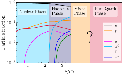
Figure 1: Particle fractions as functions of the baryonic density for the FSU2H model Tolos et al. (2017a, b) up to the point where the HQPT is implemented, giving rise to a phase of deconfined quark matter which can be separated from the nuclear (or hadronic) phase by a mixed phase of hadrons and quarks. We note that the actual fractions of nucleons/hyperons and quarks $u,d,s$ in the mixed and quark phases cannot be determined with the parametrizations used in this work.

For the hadronic phase we use the FSU2H EOS of Refs. Tolos et al. (2017a, b), which is a recent relativistic-mean field (RMF) model based on the nucleonic FSU2 model of (Chen and Piekarewicz, 2014) that considers not only nucleons but also hyperons in the inner core of neutron stars by reproducing the available hypernuclear structure data Dover and Gal (1983); Millener et al. (1988); Fukuda et al. (1998); Khaustov et al. (2000); Noumi et al. (2002); Harada and Hirabayashi (2006); Kohno et al. (2006). This scheme reconciles the $2\,M_{\odot}$ mass observations with the recent analyses of radii below 13 km for neutron stars Verbiest et al. (2008); Özel et al. (2010); Suleimanov et al. (2011); Lattimer and Lim (2013); Steiner et al. (2013); Bogdanov (2013); Guver and Özel (2013); Guillot et al. (2013); Lattimer and Steiner (2014); Poutanen et al. (2014); Heinke et al. (2014); Guillot and Rutledge (2014); Özel et al. (2016); Özel and Psaltis (2015); Lattimer and Prakash (2016); Özel and Freire (2016); Steiner et al. (2018), while fulfilling the saturation properties of nuclear matter and finite nuclei (Tsang et al., 2012; Chen and Piekarewicz, 2014), as well as the constraints extracted from nuclear collective flow (Danielewicz et al., 2002) and kaon production (Fuchs et al., 2001; Lynch et al., 2009) in heavy-ion collisions. Moreover, cooling simulations for isolated neutron stars using the FSU2H model are in very good agreement with observational data Negreiros et al. (2018).

The particle fractions as functions of the baryonic density for the FSU2H model are shown in Fig. 1 up to a density $\rho_{\rm tr}$, where the HQPT is implemented. As already seen in Refs. Tolos et al. (2017a, b); Negreiros et al. (2018), the first hyperon to appear is the $\Lambda$ particle, followed by $\Xi^{-}$ and $\Sigma^{-}$, as beta-equilibrium and charge conservation are fulfilled taking into account the most plausible hyperon potentials extracted from hypernuclear data.

II.2 High-density EOS

As the density is increased, hadrons might undergo deconfinement, liberating quarks and enabling the existence of a quark-matter core. Although the low temperature and large chemical potential regime occurring in neutron-stars interiors is still far from being well understood, two frameworks have been mainly used in the literature to describe quark matter in compact objects: the MIT bag model and the Nambu-Jona-Lasinio (NJL) model. A simpler description assuming a density-independent speed of sound mimicking these sophisticated models was first investigated in Chamel et al. (2013); Zdunik and Haensel (2013); Alford et al. (2013).

Due to its simplicity, the phenomenological CSS parametrization is well-suited for the systematic investigation of EOSs with twin stars developed in this paper. The value $c_{s}^{2}:=\partial p/\partial e={\rm const}=1$, where $p$ and $e$ are respectively the pressure and internal energy density Rezzolla and Zanotti (2013), has been previously used in Refs. Alford et al. (2013); Alford and Sedrakian (2017); Christian et al. (2018); Paschalidis et al. (2018). We have checked that the lower value $c_{s}^{2}=1/3$ provided by perturbative QCD calculations Kurkela et al. (2010) does not give rise to EOSs with twin stars that satisfy the $>2\,M_{\odot}$ maximum-mass constraint. Yet, simply setting $c^{2}_{s}=1$ allows us to carry out the extended analysis that will be presented in the following sections.

II.3 Phase Transition

The first-order transition between the hadronic and the quark phases is attained by either a Gibbs or a Maxwell construction. In the former case, the transition is modelled with a polytrope $p(\rho)=K_{\rm m}\rho^{\Gamma_{\rm m}}$ to account for a mixed soft phase of hadrons and quarks Glendenning (1992); Macher and Schaffner-Bielich (2005), and has been investigated in view of the recent gravitational-wave observations Nandi and Char (2018). The latter, on the other hand, is equivalent to a $\Gamma_{\rm m}=0$ polytrope, generates a sharp transition between the low- and high-density phases, and has been widely used in recent works, e.g., Refs. Alford et al. (2013); Christian et al. (2018); Most et al. (2018a); Paschalidis et al. (2018); Alvarez-Castillo et al. (2018); Most et al. (2018a); Han and Steiner (2018). However, if the surface tension of the deconfined quark phase has moderate values, a mixed phase between the pure hadronic and pure quark phases is expected to be present. The construction of such a continuous HQPT, where charge is only globally conserved, depends on the properties of the pure hadronic and quark models and, additionally, on possible effects of pasta structures within the mixed phase. As a result, the amount to which the EOS is softened at the beginning of the mixed phase is quite uncertain (see e.g., Ayriyan et al. (2018)) and we have used a value of $\Gamma_{\rm m}=1.03$ to mimic this effect. This choice is restricted by the fact that in our approach it is essential that $\Gamma_{\rm m}$ has a low value around 1 in order to get a strong enough softening of the EOS and to be considerably different from the Maxwell construction. We have checked that increasing/decreasing $\Gamma_{\rm m}$ by $\sim 2\%$ can shift the energy-density jump $\Delta e$ up to a $\sim 5\%$ higher/lower values at a given transition pressure $p_{\rm tr}$ of the parameter space of Model-2 discussed below. Thus the polytropic approach is a reasonable first approximation of a HQPT using the Gibbs construction and the specific choice of the value $\Gamma_{\rm m}=1.03$ does not affect significantly the discussion in the following sections.

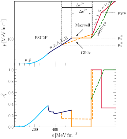
Figure 2: Upper panel: energy density as a function of the pressure corresponding to an EOS that implements a HQPT. Lower panel: The corresponding sound-speed squared in units of the speed of light. The colours are related to the composition of matter at increasing densities: $\beta$-equilibrated nucleonic matter (light blue), $\beta$-equilibrated nucleonic and hyperonic matter – hadronic matter – (dark blue), mixed phase of hadrons and deconfined quarks (orange, only Gibbs), and pure quark matter (red). Solid and dashed lines are different ways of modelling the phase transition and the quark phase (see details in the text).

II.4 Summary of the EOS models

In view of the considerations above, the adoption of the two types of phase transition will give rise to the following two models where the relation between the specific internal energy and the pressure, $e(p)$, is given by:

• Model-1: FSU2H + Maxwell + CSS

  $$e=\begin{cases}e_{\rm FSU2H}(p)&p\leq p_{\rm tr}\\ e_{\rm FSU2H}(p_{\rm tr})+\Delta e+c_{s}^{-2}(p-p_{\rm tr})&p\geq p_{\rm tr}\end{cases}$$ (1)

  with $c_{s}^{2}=1$.

• Model-2: FSU2H + Gibbs + CSS

  $$e=\begin{cases}e_{\rm FSU2H}(p)&p\leq p_{\rm tr}\\ (1+a_{\rm m})\left({p}/{K_{\rm m}}\right)^{1/\Gamma_{\rm m}}+{p}/({\Gamma_{\rm m}-1})&p_{\rm tr}\leq p\leq p_{{}_{\rm CSS}}\\ e(p_{{}_{\rm CSS}})+c_{s}^{-2}(p-p_{{}_{\rm CSS}})&p\geq p_{{}_{\rm CSS}}\end{cases}$$ (2)

  with $c_{s}^{2}=1$ and $\Gamma_{\rm m}=1.03$.

The values of the polytropic constant $K_{\rm m}$ and the coefficient $a_{\rm m}$ are obtained by ensuring that $p$ and $e$ are continuous at the transition points. We note that in the Gibbs construction an energy-density jump $\Delta e$ is not explicitly defined. In this case, we assign to its value the increase in $e(p)$ during the mixed phase (see Fig. 2).

The possible models for the EOSs are schematically shown in the upper panel of Fig. 2, where one can clearly see the comparison between Model-1^∗ and Model-2^∗ EOSs, in which the speed of sound is set to reach the perturbative QCD limit $c_{s}^{2}=1/3$ for quark matter above a certain energy density, $e(p_{\rm QCD})$, and Model-1^†, in which there is a softer EOS for the quark matter right after the phase transition. Following Refs. Paschalidis et al. (2018); Most et al. (2018a), this is modelled with a polytrope similar to that of the mixed phase [middle piece of Eq. (2) with $K_{\rm m}\rightarrow K_{\rm q}$ and $a_{\rm m}\rightarrow a_{\rm q}$, guaranteeing the continuity of $p$ and $e$ after the phase transition], which is then combined with a CSS parametrization with $c_{s}^{2}=1$ in the high-density quark phase. We note that Model-1 and Model-2 constitute a particular case of Model-1^∗ and Model-2^∗, respectively, for which the perturbative QCD limit is reached at densities higher than those in the interior of neutron stars. In the lower panel of Fig. 2 we display the square of the speed of sound (in units of the speed of light), noting that in all cases it fulfils the causal condition of $c_{s}^{2}\leq 1$.

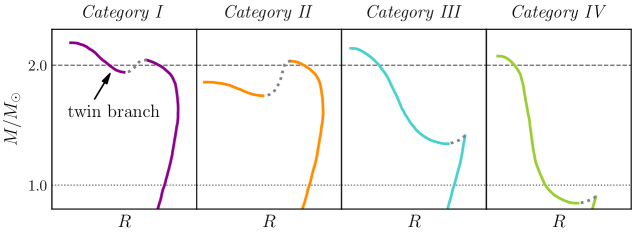
Figure 3: Schematic behaviour of the mass–radius relation for the twin-star categories I–IV defined in the text. Note the appearance of a “twin” branch with a mixed or pure-quark phase; the twin branch has systematically smaller radii than the branch with a nuclear or hadronic phase. The colours used for these categories will be employed also in the subsequent figures.

Before discussing in the next section the similarities and differences of the various models discussed above, it is useful to remark that our construction of a HQPT is not based on the “strange matter hypothesis” Bodmer (1971); Witten (1984) for which the strange-quark phase is the true ground state of elementary matter. Under such an assumption, the underlying EOS would separate in two different branches describing neutron star and pure quark matter and as a consequence, a neutron star would transform into a pure-quark star after exceeding a certain deconfinement barrier Drago et al. (2014); Bombaci et al. (2016); Lugones (2016); Burgio et al. (2018). This scenario is normally referred to as the “two-families” scenario and is different from the twin-star scenario, where the two branches of compact stars are described by a single EOS.

III Results

III.1 Parameter Space

In order to analyse the implications of the EOS models discussed in the previous section on the masses, radii and tidal deformabilities of twin-star solutions, we vary the two free parameters of the models: the density at which the phase transition to the mixed phase takes place, $\rho_{\rm tr}$, and the density discontinuity (Model-1) or density extension of the mixed phase (Model-2) up to the pure quark phase, $\Delta\rho$. This is also equivalent to setting the transition pressure, $p_{\rm tr}$, and the energy-density jump, $\Delta e$. We note that the mass density $\rho$ in the quark phase is obtained from Eqs. (1)–(2) together with the thermodynamic relation at zero temperature Rezzolla and Zanotti (2013)

$$p=\rho\frac{\partial e}{\partial\rho}-e\,,$$ (3)

so as to use the values of $\rho_{\rm QCD}$ of the order of those displayed in Fig. 7 of Ref. Tews et al. (2018b) when discussing the density at which the perturbative QCD limit is reached.

To allow for a wide range of EOSs, the parameter space analysed is $\rho_{\rm tr}\in[1.4-6.5]\,\rho_{0}$ and $\Delta\rho\in[0.2-3.0]\,\rho_{0}$ with variations of $0.1\,\rho_{0}$, where $\rho_{0}$ is the nuclear saturation density.

We recall that by using the maximum masses in the two branches, twin-star solutions can be classified in the four distinct categories shown schematically in Fig. 3:

• Category I:
  $M_{{}_{\rm TOV}}\geq 2.0\,M_{\odot}$ and $M_{{}_{\rm TOV,\,T}}\geq 2.\,M_{\odot}$

• Category II:
  $M_{{}_{\rm TOV}}\geq 2.0\,M_{\odot}$ and $M_{{}_{\rm TOV,\,T}}<2.0\,M_{\odot}$

• Category III:
  $1.0\,M_{\odot}\leq M_{{}_{\rm TOV}}<2.0\,M_{\odot}$ and $M_{{}_{\rm TOV,\,T}}\geq 2.0\,M_{\odot}$

• Category IV:
  $M_{{}_{\rm TOV}}<1.0\,M_{\odot}$ and $M_{{}_{\rm TOV,\,T}}\geq 2.0\,M_{\odot}$,

where $M_{{}_{{\rm TOV}}}$ and $M_{{}_{\rm TOV,\,T}}$ are the maximum masses of the branches with large (“normal-neutron-star” branch) and small radii (“twin” branch), respectively, of a nonrotating neutron star obtained by solving the Tolman-Oppenheimer-Volkoff (TOV) equations. Since our aim is to focus on those configurations that allow for maximum masses larger than $2\,M_{\odot}$ while having a twin-star solution, we will not consider those cases where the EOSs lead to twin-star solutions that violate the $M_{{}_{\rm TOV}}^{{}^{\uparrow}}:=\max\{M_{{}_{\rm TOV}},M_{{}_{\rm TOV,\,T}}\}\geq 2.0\,M_{\odot}$ constraint. Similarly, EOSs that do not produce twin stars will also be rejected from our analysis.

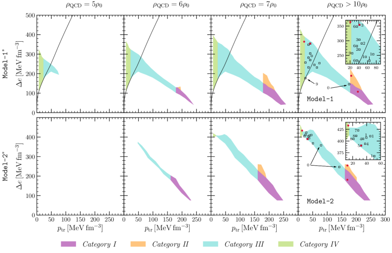
Figure 4: Areas containing the various categories of twin stars in the $\Delta e$–$p_{\rm tr}$ parameter space for EOS models with Maxwell construction (upper panels) and models with Gibbs construction (lower panels) for the phase transition, and increasing values of the density $\rho_{\rm QCD}$ corresponding to the onset of the perturbative QCD limit, $c_{s}=1/\sqrt{3}$, labelled Model-1^∗ and Model-2^∗ in the text. The Model-1 and Model-2 EOSs are depicted in the rightmost upper and lower panels, respectively. The solid line in the upper panels is the Seidov limit of Eq. (4). Circles, squares and numbers identify the specific cases studied in the figures in the rest of the paper and are also shown in the magnified insets.

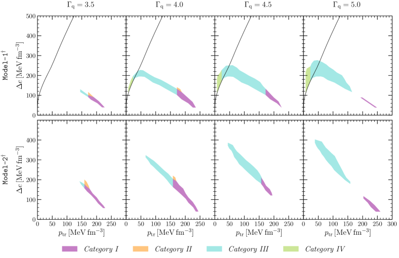
Figure 5: Areas containing the various categories of twin stars in the $\Delta e$–$p_{\rm tr}$ parameter space for Model-1^† with a Maxwell (upper panels) and Model-2^† with a Gibbs (lower panels) phase transition, that use for the quark phase a polytrope $p(\rho)=K_{\rm q}\rho^{\Gamma_{\rm q}}$ combined with a constant speed of sound parametrization when the speed of sound $c_{s}^{2}=\partial p/\partial e$ reaches the value of one. The value of the polytropic index $\Gamma_{\rm q}$ is varied between 3.5 to 5.0, so as to obtain twin-star solutions and masses $M\geq 2.0\,M_{\odot}$. The solid line in the upper panels is the Seidov limit of Eq. (4).

Figure 4 shows the parameter space in the $\Delta e$–$p_{\rm tr}$ plane for EOS models having either a Maxwell construction (Model-1^∗, upper panels) or a Gibbs construction (Model-2^∗, lower panels) for the phase transition. From the left to the right, we vary the density $\rho_{\rm QCD}$ at which the asymptotic perturbative $c_{s}^{2}=1/3$ limit in the quark-matter phase is reached.

Only the combinations of parameters within the shaded regions correspond to EOSs that allow for a twin-star configuration together with $M_{{}_{\rm TOV}}^{{}^{\uparrow}}\geq 2.0\,M_{\odot}$, with different colours referring to Categories I-IV. We note that the allowed parameter space is determined by the intersection of the two regions satisfying each of these conditions, the boundaries of which are similar to those shown in Fig. 2 of Ref. Alford et al. (2015) with a Maxwell construction. The solid line in the top panels of Fig. 4 corresponds to the limiting condition for hybrid stars appearing in the normal-neutron-star branch, which can be derived solely in the presence of a sharp discontinuity in the energy density by performing an expansion in powers of the size of the quark-matter core Seidov (1971); Schaeffer et al. (1983); Lindblom (1998); Alford et al. (2013), written in the following form:

$$\Delta e=\frac{1}{2}e_{\rm tr}+\frac{3}{2}p_{\rm tr}\,.$$ (4)

For combinations of parameters above the Seidov line (4), the sequence of stars will become unstable immediately after the central pressure reaches the value $p_{\rm c}=p_{\rm tr}$, i.e., the stars in the normal-neutron-star branch will be purely hadronic, while the combinations below the line correspond to solutions for which the normal-neutron-star branch can support hybrid stars (with quark core) before turning unstable. Note also that the circles and squares in the figure identify the specific cases studied more in detail below.

When inspecting Fig. 4 it is evident that Model-1 and Model-2 are the most effective EOSs in fulfilling both requirements, as shown by the corresponding largest coverage of the $\Delta e$–$p_{\rm tr}$ parameter space. Moreover, since it is not yet clear at what value of $\rho_{\rm QCD}/\rho_{0}$ the asymptotic perturbative QCD limit takes place, our analysis hereafter will be focused on Model-1 and Model-2 EOSs only. For these two cases, Categories I (purple areas) and III (blue) are easily produced. Twin-star solutions of Category II (orange) also appear in both models, although the area filled in the parameter space is rather small, while twin stars of Category IV (green) are abundant for the Model-1 EOSs, but become more difficult to be found for Model-2 having the Gibbs construction.

By analysing Model-1 [Model-2] EOSs we observe that, in order to reach $2\,M_{\odot}$ in the normal-neutron-star branch for Categories I-II, we need $p_{\rm tr}>180~{}\rm MeV\,fm^{-3}\;[160~{}\rm MeV\,fm^{-3}]$. Twin-star solutions of Category II are located in the same range of $p_{\rm tr}$ occupied by those of Category I (see Fig. 4), but at slightly higher values of $\Delta e$. We recall that the two classes of solutions differ in whether the twin branch is above (Category I) or below (Category II) the $2\,M_{\odot}$ value (see Fig. 3). In fact, using our two EOS models, these two categories are difficult to be differentiated since the values of the maximum masses for the two branches lie within a rather small range, i.e., $1.95\,M_{\odot}\lesssim M_{{}_{\rm TOV,\,T}}\lesssim 2.05\,M_{\odot}$.

Twin-star solutions of Category IV appear for very low values of $p_{\rm tr}$ (i.e., $p_{\rm tr}\lesssim 25\rm\,MeV\,fm^{-3}\;[15\rm\,MeV\,fm^{-3}]$), as required in order for the maximum mass of the normal-neutron-star branch to be below the $1\,M_{\odot}$ value. Twin stars of this category might not exist because the mass in the normal-neutron-star branch is much lower than the canonical value of $1.4\,M_{\odot}$, which should be well described as normal neutron stars, given our present knowledge of nuclear matter at the expected central densities.

Also clear from Fig. 4 is that the category that contains the largest number of twin-star solutions is Category III, with ${25\rm\,MeV\,fm^{-3}}\lesssim p_{\rm tr}\lesssim 180\rm\,MeV\,fm^{-3}$  [${15\rm\,MeV\,fm^{-3}}\lesssim p_{\rm tr}\lesssim 160\rm\,MeV\,fm^{-3}$] and the width of the $\Delta e$ range depending on the model for the EOS. In addition, Category III is certainly the most interesting category from an astrophysical point of view, as it accommodates twin stars of masses around the canonical $1.4\,M_{\odot}$ value.

Finally, we show in Fig. 5 the $\Delta e$–$p_{\rm tr}$ parameter space for Model-1^† (upper panels) and Model-2^† (lower panels), with a Maxwell and Gibbs phase transition, respectively, that implement for the quark phase a polytrope $p(\rho)=K_{\rm q}\rho^{\Gamma_{\rm q}}$, combined with a constant speed of sound parametrization when $c_{s}^{2}=1$. In this case, we find that the parameter space increases with increasing polytropic index. The higher the polytropic index, the stiffer the EOS and, hence, the easier it is to find twin-star solutions with $M_{{}_{\rm TOV}}^{{}^{\uparrow}}\geq 2.0\,M_{\odot}$. By comparing the $\Delta e$–$p_{\rm tr}$ parameter space of Model-1 and Model-2 EOSs in Fig. 4 with the corresponding space in Fig. 5, we conclude that EOSs of Model-1 and Model-2 are still the most effective in providing twin-star configurations and masses $\geq 2.0\,M_{\odot}$.

III.2 Masses and Radii

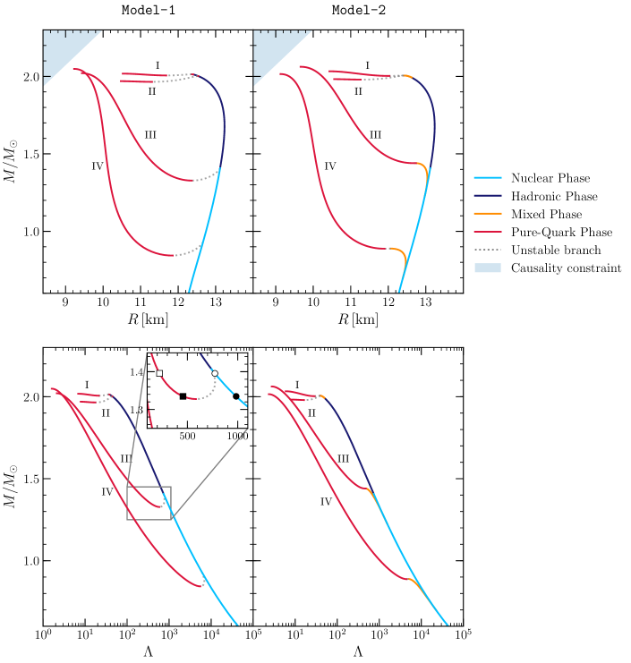
Figure 6: Upper panels: Selected mass–radius relations classified in the corresponding twin-star category for Model-1 and Model-2. The grey dotted lines correspond to the unstable regions. The light-blue shaded area marks the causality limit for compactness $R\geq 2.94~{}M$. Lower panels: Dimensionless tidal deformability $\Lambda$ of a single neutron star as a function of its mass using the same EOSs as in the upper panels. The colouring indicates the composition of the innermost region of the neutron star (nucleons, nucleons and hyperons, mixed phase and pure-quark phase) at a central density $\rho_{c}$, as seen in Fig. 2. The symbols in the inset represent the possible configurations of binaries with masses $M_{1}\gtrsim M_{2}$ set by the GW170817 chirp mass $\mathcal{M}=1.188\,M_{\odot}$: circles for neutron stars in the hadronic branch and squares for hybrid stars in the twin branch; empty symbols for the high-mass component of the binary and filled symbols for the low-mass one.

A selection of the possible $M$–$R$ relations obtained for Model-1 and Model-2 EOSs is displayed in the upper two panels of Fig. 6. Each curve in a given panel shows the $M$–$R$ relation for a given twin-star category, with the corresponding values of $\Delta e$ and $p_{\rm tr}$ being provided in the rightmost upper and lower panels of Fig. 4, where the red circles single out the values plotted in Fig. 6. Note that by using the same colour palette as in Fig. 2, we show with different colours in the various $M$–$R$ curves the composition of the innermost region of the star: light blue for neutron stars entirely composed of nucleonic matter, dark blue if the central pressure is large enough to allow for the appearance of hyperons, orange if there is an inner core of mixed matter surrounded by a hadronic- (or nuclear-) matter mantle, and red for the hybrid star composed of a quark-matter core and a mantle of hadronic (or nuclear) matter, separated by a mixed-phase region within Model-2. Dashed lines in grey correspond to unstable configurations.

Model		Normal-neutron-star branch			Twin branch
		$M_{{}_{\rm TOV}}~{}[M_{\odot}]$	$R_{1.4}\rm~{}[km]$	$\Lambda_{1.4}$	$M_{{}_{\rm TOV,T}}~{}[M_{\odot}]$	$R_{1.4}\rm~{}[km]$	$\Lambda_{1.4}$
Maxwell	Model-1	$[1.06,\,2.00)$	$13.1$	$760$	$[2.00,\,2.44]$	$[10.1,\,12.9]$	$[69,\,609]$
	$\rho_{\rm QCD}=5\rho_{0}$	$[1.06,\,1.76]$	$13.1$	$760$	$[2.00,\,2.38]$	$[11.1,\,12.9]$	$[149,\,609]$
	$\Gamma_{\rm q}=4.0$	$[1.06,\,2.00)$	$13.1$	$760$	$[2.00,\,2.05]$	$[11.0,\,12.9]$	$[145,\,599]$
Gibbs	Model-2	$[1.02,\,2.00)$	$[12.9,\,13.1]$	$[679,\,760]$	$[2.00,\,2.08]$	$[10.4,\,11.9]$	$[114,\,295]$
	$\rho_{\rm QCD}=6\rho_{0}$	$[1.72,\,1.99]$	$13.1$	$760$	$[2.00,\,2.02]$	$-$	$-$
	$\Gamma_{\rm q}=4.0$	$[1.84,\,2.00)$	$13.1$	$760$	$[2.00,\,2.03]$	$-$	$-$

Table 1: Physical properties of the stars of Category III obtained within the most representative models described in the text.

With these considerations, one can readily appreciate the multiplicity of possibilities concerning masses, radii and internal structures for each of the twin stars obtained with our two EOS models. We note that for Categories I-II, the allowed $p_{\rm tr}\gtrsim 160~{}\rm MeV\,fm^{-3}$ region seen in Fig. 4 results in a nearly flat twin mass–radius branch, as noted in Ref. Christian et al. (2018). Also, for values of $p_{\rm tr}$ similar to those in Category I, higher values of $\Delta e$ in Category II (see Fig. 4) are responsible for unstable regions separating the two stable branches that are larger in Category II than in Category I. This is due to the fact that a larger $\Delta e$ produces heavier quark cores, with the subsequent greater gravitational pull on the nuclear mantle, so that the twin branch takes longer to stabilize Macher and Schaffner-Bielich (2005); Alford et al. (2013).

An interesting quantity to consider across the different twin-star categories and the EOS models is the radius difference between the two equal-mass twin stars, $\Delta R$. In Ref. Christian et al. (2018) values of $\Delta R$ as large as $4\,{\rm km}$ were claimed to be possible. This radius difference would allow for the distinction of the two stars given that a few per cent accuracy might be expected in future determinations of the radius, either via electromagnetic emissions (Watts et al., 2016) or via gravitational waves Bose et al. (2018). However, we here find that the largest differences are $\Delta R\sim 2.7\,{\rm km}$ and $\Delta R\sim 2.3\,{\rm km}$, that correspond to twin stars of Categories IV and II, respectively, in the Model-1 EOSs, and $\Delta R\sim 2.2\,{\rm km}$ for Category II in Model-2. This is most certainly due to the different hadronic EOS here, which is softer than that employed in Christian et al. (2018). Finally, we note that for Category III, which is possibly the most interesting case as it can accommodate twin stars with masses around $1.4\,M_{\odot}$, the largest difference in radii is $\Delta R\sim 1.9\,{\rm km}$ and $\Delta R\sim 1.4\,{\rm km}$ in the case of Model-1 and Model-2, respectively, thus making it more difficult to distinguish the two types of stars.

III.3 Tidal deformabilities

The tidal deformability is a property of the EOS that is in principle measurable via gravitational-wave observations of binary neutron-star inspirals, as done with the recent GW170817 event Abbott et al. (2017). It is therefore interesting to explore the behaviour of the tidal deformability for different EOSs that allow for the appearance of twin stars. This is done in the lower panels of Fig. 6, which report the dimensionless tidal deformability $\Lambda$ as a function of the mass of the neutron star for the same selection of EOSs as in the upper panels. From the figure it is clearly seen that $\Lambda$ spans several orders of magnitude for different EOSs.

With regards to the dimensionless tidal deformability for the reference star with a mass of $1.4\,M_{\odot}$, i.e., $\Lambda_{1.4}$, we observe a considerable difference between EOSs that exhibit a phase transition at low densities (such as Category IV) and at high densities (Categories I-II) for the two models considered. More specifically, a reference $1.4\,M_{\odot}$ star with a dense core of quark matter in Category IV has $\Lambda_{1.4}$ ranging from a few tens to a few hundreds, while a $1.4\,M_{\odot}$ pure hadronic neutron star in Categories I-II has $\Lambda_{1.4}=760$. The differences in the values of $\Lambda_{1.4}$ can be explained by the different compactnesses of the stars. We recall, in fact, that $\Lambda\propto k_{2}\mathcal{C}^{-5}$, where $\mathcal{C}:=M/R$ is the stellar compactness and $k_{2}$ the second tidal Love number. On the other hand, $k_{2}\propto\mathcal{C}^{-1}$ in the mass range of typical neutron stars Hinderer et al. (2010); Zhao and Lattimer (2018), so that $\Lambda\propto\mathcal{C}^{-6}$. In the presence of a HQPT, however, this correlation is expected to be weakened Postnikov et al. (2010). At any rate, for the same total mass of $1.4\,M_{\odot}$, stars with a quark-matter core have smaller radii and, hence, larger compactness or, equivalently, smaller values of $\Lambda_{1.4}$.

When considering the case of Category III, we obtain twin stars with masses around $1.4\,M_{\odot}$. These configurations have a core of mixed or pure quark matter with a radius for the star between the radius for Categories I-II and Category IV. Thus, the value of $\Lambda_{1.4}$ lies between the values for $\Lambda_{1.4}$ in Categories I-II and Category IV. The inset in the left panel shows in greater detail the behaviour of $\Lambda(M)$ around the phase transition for an EOS of Category III that is of particular interest because it holds stars with masses of $1.365\,M_{\odot}$ in both branches and will be further discussed in Section III.4.

We note that using the detection of GW170817, Ref. Abbott et al. (2017) derived an upper bound $\Lambda_{1.4}\leq 800$ (corrected later to $\leq 900$) upon the GW170817 event, that was later on reanalysed to be $300^{+420}_{-230}$ Abbott et al. (2019). However we note that this constraint is obtained by expanding $\Lambda(M)$ linearly about $M=1.4\,M_{\odot}$, and from Fig. 6 we can see that if the twin branch appears at $M\sim 1.4\,M_{\odot}$ this approach is no longer valid and the upper bound on $\Lambda_{1.4}$ could be further decreased, as shown in Refs. Most et al. (2018a); Paschalidis et al. (2018); Burgio et al. (2018). In fact, Ref. Most et al. (2018a) has shown that the lower limit on $\Lambda_{1.4}$ is decreased from $\Lambda_{1.4}\geq 375$ to $\Lambda_{1.4}\geq 265$ at $2$-$\sigma$ level (see the supplemental material of Ref. Most et al. (2018a)) when allowing for a phase transition.

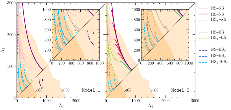
Figure 7: Relation between the tidal deformabilities of the high-mass and the low-mass components, $\Lambda_{1}$ and $\Lambda_{2}$, of a binary neutron star with a chirp mass $\mathcal{M}=1.188\,M_{\odot}$ for Model-1 and Model-2 EOSs of Category III only. The colours are related to the nature of each of the components of the $M_{1}$–$M_{2}$ binary system: NS for a hadronic or pure neutron star, HS for a hybrid star in the normal-neutron-star branch, and HS${}_{{}_{\rm T}}$ for a hybrid star in the twin branch, with the first label referring to the massive component of the binary ($M_{1}$) and the second to the less massive ($M_{2}$) separated by a long dash. The lines displayed correspond to the EOSs indicated with empty squares in Fig. 4, each EOS giving a unique “connection” among NS, HS and HS${}_{{}_{\rm T}}$ in the $\Lambda_{1}$–$\Lambda_{2}$ plane: 0. (NS–NS), 1. (NS–NS, HS–NS, HS${}_{{}_{\rm T}}$–NS), 2. (NS–NS, HS${}_{{}_{\rm T}}$–NS), 3. (NS–NS, HS${}_{{}_{\rm T}}$–NS, HS${}_{{}_{\rm T}}$–HS${}_{{}_{\rm T}}$, NS–HS${}_{{}_{\rm T}}$), 4. (HS–HS, HS–NS, HS${}_{{}_{\rm T}}$–NS), 5. (HS–HS, HS${}_{{}_{\rm T}}$–HS, HS${}_{{}_{\rm T}}$–NS), 6. (HS${}_{{}_{\rm T}}$–HS${}_{{}_{\rm T}}$, HS${}_{{}_{\rm T}}$–NS), 7. (HS${}_{{}_{\rm T}}$–HS${}_{{}_{\rm T}}$, HS${}_{{}_{\rm T}}$–HS, HS${}_{{}_{\rm T}}$–NS), 8. (HS${}_{{}_{\rm T}}$–HS${}_{{}_{\rm T}}$, HS${}_{{}_{\rm T}}$–HS), 9. (HS${}_{{}_{\rm T}}$–HS${}_{{}_{\rm T}}$). The shaded areas correspond to the 50% and 90% credibility regions set by GW170817 for a low-spin scenario $|\chi|\leq 0.05$ Abbott et al. (2017). The inset also reports for comparison the tidal deformabilities of representative nucleonic EOSs (grey lines).

In Table 1 we report the range of values for the maximum mass, radius ($R_{1.4}$) and tidal deformability for a $1.4\,M_{\odot}$ star for Model-1 and Model-2 EOSs in Category III, both in the normal and in the twin branch. Moreover, for completeness, we also show the ranges for these quantities coming from four representative EOS models, that have been computed using the Maxwell or Gibbs construction for the phase transition and taking into account the two different descriptions of the quark-matter phase discussed in Section III.1. We observe a larger variance for $R_{1.4}$ and $\Lambda_{1.4},$ for both Model-1 and Model-2 EOSs in both branches, which can be understood in terms of the larger $\Delta e$–$p_{\rm tr}$ space of parameters (cf., Sec. III.1). Thus, as mentioned before, we will restrict our attention to Model-1 and Model-2 EOSs when performing the analysis of the tidal deformabilities of neutron-star binaries.

III.4 Tidal deformabilities and GW170817

In order to compare directly with the observational analysis from the GW170817 event Abbott et al. (2017), we considered a binary system with a chirp mass $\mathcal{M}:=(M_{1}M_{2})^{3/5}/(M_{1}+M_{2})^{1/5}=1.188\,M_{\odot}$ and calculated the tidal deformabilities $\Lambda_{1}$ and $\Lambda_{2}$ of the high-mass $M_{1}$ and low-mass $M_{2}$ components, respectively, plotting the 50% and 90% credibility regions for the low-spin scenario $|\chi|\leq 0.05$ given in Refs. Abbott et al. (2017, 2018). This is shown in Fig. 7 for selected EOSs with twin stars of Category III only within Model-1 and Model-2 EOSs. Lines of different colour and type show different number of branches and shapes in the $\Lambda_{1}$–$\Lambda_{2}$ plane obtained by varying $M_{1}\in[1.365,1.8]\,M_{\odot}$ and $M_{2}\in[1.0,1.365]\,M_{\odot}$ (with fixed $\mathcal{M}=1.188\,M_{\odot}$). The corresponding values of $\Delta e$ and $p_{\rm tr}$ of the selected EOSs are indicated with black empty squares in the rightmost upper and lower panels of Fig. 4.

The different colour lines in Fig. 7 are related to the nature of each of the components, with the labels having the following meaning: NS for a purely hadronic neutron star, HS for a hybrid star with a core of mixed and/or quark matter in the “normal-neutron-star” branch, and HS${}_{{}_{\rm T}}$ for a hybrid star with a quark core in the “twin” branch, with the first label referring to the massive component of the binary ($M_{1}$) and the second to the less massive ($M_{2}$) separated by a long dash. Allowing for all these possibilities, there can be up to eight lines in the $\Lambda_{1}$–$\Lambda_{2}$ plane (see legend of Fig. 7). However, not all of them are produced by each of the EOS models at a given $\mathcal{M}$.

This is reported in Fig. 8, which shows the minimum value of the chirp mass for which at least one of the components of the binary before the merger is in the twin branch as a function of the values of the transition pressure and energy-density jump of the EOSs of Category III for the Model-1 EOSs (upper panels); left and right panels refer to mass ratios of $q=1.0$ and $q=0.7$, respectively. In full similarity, same quantities are shown in the lower panels for the Model-2 EOSs.

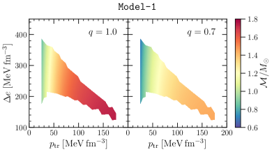
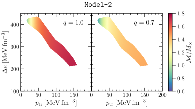
Figure 8: Upper panels: Minimum value of the chirp mass for which at least one of the components of the binary is in the twin branch, shown as a function of the values of the transition pressure and energy-density jump of the EOSs of Category III for the Model-1 EOSs for $q=1$ (left panel) and $q=0.7$ (right panel). Lower panels: Same as upper panels but for the Model-2 EOSs.

As expected, the lower the transition pressure, the lower the minimum chirp mass required for the HQPT to occur in at least one of the stars in the binary given that it is easier to populate the twin branch for low transition pressures. Note that the lowest value for the chirp mass is $0.6\,M_{\odot}$ and that for $q=1$ higher chirp masses are needed to have one of the components in the twin branch when compared with the $q=0.7$ case. This is because for unequal-mass binaries, it is easier for the high-mass component to be on the twin branch.

For the EOSs that allow for twin stars of Categories I-II (not shown in Fig. 7), for which the mass of the twins is significantly larger than that of the components in GW170817, only the hadronic part of the EOS is reported for $\Lambda_{i}\in[0,3000]$ and only the NS–NS (purple) line is shown. The opposite limiting case corresponds to EOSs that allow for twin stars of Category IV (not shown in Fig. 7) and hence with very low masses. For this case, both components of the binary system are located in the twin branch, producing only lines of the type HS${}_{{}_{\rm T}}$–HS${}_{{}_{\rm T}}$ (light blue) in the $\Lambda_{1}$–$\Lambda_{2}$ plot, with $\Lambda_{1}<200$ for both models. On the other hand, in the case of EOSs with twins stars of Category III, the range of possibilities is larger, mostly due to the existence of twin stars with masses similar to those of the GW170817 binary ($M_{1}=M_{2}=1.365\,M_{\odot}$ in the equal-mass limit). Indeed, as shown in Fig. 7, Model-1 and Model-2 EOSs show clear differences with regards to the number of possible scenarios.

The general considerations made above can be made more specific starting, in particular, from EOSs of Model-1 (left panel of Fig. 7).

In this case, for an EOS with a HQPT at high transition pressure (i.e., with $p_{\rm tr}\gtrsim 80\rm\,MeV\,fm^{-3}$ in Fig. 4, which corresponds to $\rho_{\rm tr}\gtrsim 3\,\rho_{0}$), only the NS–NS sequence (purple line) is found. If the phase transition takes place at lower densities ($2.2\,\rho_{0}\lesssim\rho_{\rm tr}\lesssim 3.0\,\rho_{0}$, i.e., $40{\rm\,MeV\,fm^{-3}}\lesssim p_{\rm tr}\lesssim 80\rm\,MeV\,fm^{-3}$), the twin branch contains hybrid stars with a mass that is low enough to hold the high-mass component of the binary. In this case, when $M_{1}\approx M_{2}$ both stars are in the normal-neutron-star branch, but as $M_{1}$ is increased (and $M_{2}$ decreased to keep $\mathcal{M}$ constant) it jumps to the twin branch and the NS–NS sequence (purple line) connects with a HS${}_{{}_{\rm T}}$–NS (pink lines) line. On the other hand, the normal-neutron-star branch of EOSs with low transition pressure ($p_{\rm tr}\lesssim 25\rm\,MeV\,fm^{-3}$ in Fig. 4, i.e., $\rho_{\rm tr}\lesssim 1.9\,\rho_{0}$) cannot support any of the components of the binary and the only allowed configuration is HS${}_{{}_{\rm T}}$–HS${}_{{}_{\rm T}}$ (light blue lines). Larger values of $p_{\rm tr}$ ($30{\rm\,MeV\,fm^{-3}}\lesssim p_{\rm tr}\lesssim 40\rm\,MeV\,fm^{-3}$, i.e., $2.0\,\rho_{0}\lesssim\rho_{\rm tr}\lesssim 2.2\,\rho_{0}$) allow the low-mass component to be a neutron star. This situation corresponds to having the two components in the twin branch when their masses are equal and the low-mass star jumps to the normal-neutron-star branch as $M_{2}$ is decreased, giving a HS${}_{{}_{\rm T}}$–NS (pink lines) line connecting with the HS${}_{{}_{\rm T}}$–HS${}_{{}_{\rm T}}$ sequence (light blue lines).

There is in addition a particular case in which the value $M_{1}=M_{2}=1.365\,M_{\odot}$ is contained within the range of masses of the twin stars produced. This is indeed what happens for some EOSs in Model-1, as it can be appreciated in the inset of the third panel in Fig. 6. In this case, we can have both components of the binary in the normal-neutron-star branch (marked as $\circ$ and $\bullet$ in Fig. 6), both in the twin branch ($\square$ and $\blacksquare$ in Fig. 6); alternatively, we can have the high-mass star in the twin branch and the low-mass star in the normal-neutron-star branch ($\square$ and $\bullet$ in Fig. 6) and also the high-mass star in the normal-neutron-star branch and the low-mass star in the twin branch ($\circ$ and $\blacksquare$ in Fig. 6). These configurations are marked in the left panel of Fig. 7 respectively as: NS–NS (purple lines), HS${}_{{}_{\rm T}}$–HS${}_{{}_{\rm T}}$ (dashed light-blue lines), HS${}_{{}_{\rm T}}$–NS (dashed pink lines) and NS–HS${}_{{}_{\rm T}}$ (dashed dark-blue lines).

Also noticeable is that this last extra NS–HS${}_{{}_{\rm T}}$ sequences (dashed dark-blue lines) appear in the otherwise empty $\Lambda_{1}>\Lambda_{2}$ region. For EOSs not producing twin stars and given that $M_{1}>M_{2}$, one has $\mathcal{C}_{1}>\mathcal{C}_{2}$ and, hence, $\Lambda_{1}<\Lambda_{2}$, so it is usually not possible to have solutions in the $\Lambda_{1}>\Lambda_{2}$ area. However, this does not hold for EOSs giving rise to twin stars, since in this case the high-mass star can be less compact than the low-mass one, as seen in the inset of Fig. 6 for the $\circ$ and $\blacksquare$ cases. This type of pairs, where the heavier star is also less compact, has been named “rising-twins” pair in Ref. Schertler et al. (2000); by definition, therefore, rising twins can only appear with EOSs that allow for twin stars and their existence is not allowed by any other kind of EOS of compact stars. In summary, if the EOS allows for rising twins of masses $M_{1}$ and $M_{2}<M_{1}$, tied together by a given value of the chirp mass $\mathcal{M}$, there must be a line in the $\Lambda_{1}>\Lambda_{2}$ side of the plot. Indeed, in Ref. Christian et al. (2019) it was suggested that this is the case so long as $0<(M_{1}-M_{2})/(R_{1}-R_{2})<M_{1}/R_{1}$.

As a consequence, since only EOSs producing twin stars can access the region with $\Lambda_{1}>\Lambda_{2}$ for $M_{1}>M_{2}$, any experimental indication that the binary occupies this region of the $\Lambda_{1}$–$\Lambda_{2}$ space would be a strong evidence for the existence of twin stars. Other EOSs with a HQPT but not generating twin stars would show similar lines in the $\Lambda_{1}<\Lambda_{2}$ region as those displayed in the left panel of Fig. 7. In this case, one might expect all the lines of stable configurations connected to one another, but the $\Lambda_{1}>\Lambda_{2}$ would be unattainable. This situation was analysed in Ref. Sieniawska et al. (2018) for polytropic EOSs with a CSS parametrization of the quark phase and different values of the energy-density jump. However, to find such a signature in the $\Lambda_{1}$–$\Lambda_{2}$ plot is very challenging as it requires a modeling of the LIGO/Virgo data that includes a phase transition and more accurate measurements of the component masses, since in our models the twin stars have similar masses in this region.

A similar discussion can be made for the Model-2 EOSs and is shown in the right panel of Fig. 7. The variety of lines (colours) increases because the probability of having a HS in the normal-neutron-star branch is higher than for Model-1. In the Maxwell construction, for combinations of phase transition parameters below the Seidov line [see Eq. (4)], the normal-neutron-star branch is composed of a hybrid segment connected to the purely-hadronic segment whose length is typically quite small and hence hard to capture in the right panel of Fig. 7. On the other hand, in the Gibbs construction, hybrid stars with a core of hadron-quark mixed phase can be found in a relevant portion of the normal-neutron-branch, as shown in Fig. 6. Several previous works have also studied the possibility of interpreting the GW170817 event as the coalescence of pure neutron stars and hybrid stars Paschalidis et al. (2018); Nandi and Char (2018); Alvarez-Castillo et al. (2018); Burgio et al. (2018); Sieniawska et al. (2018); Li et al. (2018); Gomes et al. (2018); Christian et al. (2019); Han and Steiner (2018), although only some of them considered the possibility of twin stars Paschalidis et al. (2018); Alvarez-Castillo et al. (2018); Burgio et al. (2018); Sieniawska et al. (2018); Christian et al. (2019). In Ref. Paschalidis et al. (2018), in particular, NS–NS and HS${}_{{}_{\rm T}}$–NS merger combinations were considered. It was then shown that a HQPT can soften the EOS making it compatible, even for a stiff hadronic EOS, with the GW170817 observations. In particular, the authors found that GW170817 is consistent with the coalescence of a HS${}_{{}_{\rm T}}$–NS binary.

Similarly, in Ref. Alvarez-Castillo et al. (2018), the GW170817 event was interpreted as the merger of either a HS${}_{{}_{\rm T}}$–NS or a HS${}_{{}_{\rm T}}$–HS${}_{{}_{\rm T}}$ binary and actually disfavoured a NS–NS scenario. This was mostly due to the stiffness of the hadronic EOS employed, that made a neutron-star merger incompatible with the compactness expected from GW170817. More recently, Ref. Christian et al. (2019) has interpreted the GW170817 event as the merger scenario of either a NS–NS, a NS–HS${}_{{}_{\rm T}}$, or HS${}_{{}_{\rm T}}$–HS${}_{{}_{\rm T}}$ binary, where all three merger scenarios can be potentially plausible within a single EOS. This finding is in agreement with the conclusions presented here, although in our study we have performed a more detailed analysis of the merger scenarios in which we have also varied the parameters characterizing the phase transition (i.e., $\Delta e$ and $p_{\rm tr}$), while considering both Maxwell and Gibbs constructions for the phase transition, i.e., having a significant number of HS configurations in addition to NS and HS${}_{{}_{\rm T}}$ configurations.

Finally, Ref. Han and Steiner (2018) has very recently explored the sensitivity of the tidal deformability to the properties of a sharp HQPT, not necessarily producing twin stars, finding that a smoothing of the transition will not have distinguishable effects. In our case, when twin-star solutions and masses above $2\,M_{\odot}$ are produced, we find however clear differences in masses, radii and tidal deformabilities when comparing our Model-1 and Model-2 EOSs in Figs. 4, 6 and 7. This is due to the “smoothing” of the mixed phase between the Maxwell and Gibbs constructions, which is different from that of the rapid crossover transition in Ref. Han and Steiner (2018), and that leads to the rather different behaviour of the speed of sound in the two cases.

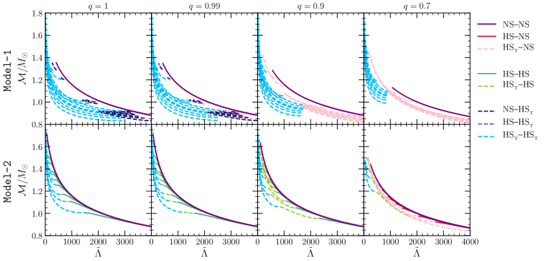
Figure 9: Relation between the chirp mass, $\mathcal{M}$, and the dimensionless tidal deformability, $\tilde{\Lambda}$, of binary systems with mass ratios $q=1,0.99,0.9,0.7$ for the same Model-1 (upper panels) and Model-2 (lower panels) EOSs of Category III shown in 7

.

In order to distinguish the different kinds of compact star merger scenarios that are compatible with future gravitational wave events, a more promising tool would be to analyse the chirp mass, $\mathcal{M}$, as a function of the weighted dimensionless tidal deformability $\tilde{\Lambda}$ of a neutron-star binary Flanagan and Hinderer (2008); Favata (2014); Abbott et al. (2017)

$$\tilde{\Lambda} := \frac{8}{13}[(1+7\eta-31\eta^{2})(\Lambda_{1}+\Lambda_{2})$$

$$+\sqrt{1-4\eta}(1+9\eta-11\eta^{2})(\Lambda_{1}-\Lambda_{2})$$

$$= \frac{16}{13M^{5}}[(M_{1}+12M_{2})M_{1}^{4}\Lambda_{1}+(M_{2}+12M_{1})M_{2}^{4}\Lambda_{2}]\,,$$

where $\eta:=M_{1}M_{2}/M^{2}$ is the symmetric mass ratio, $M:=M_{1}+M_{2}$ is the total mass of the binary, and where, in the equal-mass case, $\tilde{\Lambda}=\Lambda$.

Figure 9 displays the relation $\mathcal{M}$–$\tilde{\Lambda}$ for different values of the mass ratio, $q$, for the selected Model-1 (upper panels) and Model-2 (lower panels) EOSs with twin stars of Category III shown in the $\Lambda_{1}$–$\Lambda_{2}$ plot of Fig. 7 and using the same colour palette to refer to the various merger scenarios. We can see that the merger of rising twins happens for mass ratios $q\lesssim 1$. However, rising twins cannot be identified in Fig. 9 because, due to the symmetry of $\tilde{\Lambda}$ with respect to the two components of the binary [see Eq. (III.4)], for $q=1$ the HS${}_{{}_{\rm T}}$–NS sequence (dashed pink line) overlaps exactly with the NS–HS${}_{{}_{\rm T}}$ rising twins (dashed dark-blue line) in the leftmost upper panel, and the HS${}_{{}_{\rm T}}$–HS sequence (dashed light-green line) lies on top of the HS–HS${}_{{}_{\rm T}}$ rising twins (dashed medium-blue line) in the leftmost lower panel. With a small asymmetry ($q=0.99$) these lines do not exactly overlap each other but still lie in the same region of the $\mathcal{M}$–$\tilde{\Lambda}$ plot. We also note that the rising twins extend over a larger range of $\mathcal{M}$ and $q$ in Model-1 than in Model-2 because the larger unstable branches in the $M$–$R$ relation obtained with the Maxwell construction of the HQPT allow for broader ranges of twin stars (see Fig. 6) than the Gibbs construction. Also from Fig. 9 it is clear that within our description, the possibility of having a merger of two hybrid stars in the twin branch (i.e., HS${}_{{}_{\rm T}}$–HS${}_{{}_{\rm T}}$) diminishes with decreasing values of $q$ in favor of either the HS${}_{{}_{\rm T}}$–NS scenario in the case of Model-1 or the HS${}_{{}_{\rm T}}$–NS and HS${}_{{}_{\rm T}}$–HS scenarios in the case of Model-2. Indeed at large asymmetries (e.g., $q=0.7$) the merger of two hybrid stars with a chirp mass $\mathcal{M}\lesssim 1\,M_{\odot}$ is ruled out in our models because the twin branch cannot hold the low-mass star. Therefore, the analysis above reveals that within our models the merger scenario can be readily determined given a measure of the chirp mass and the weighted dimensionless tidal deformability.

III.5 Constraining twin stars with GW170817

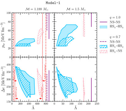
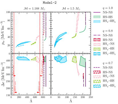
Figure 10: Left plot: Transition pressure $p_{\rm tr}$ (upper panels) and energy-density jump $\Delta e$ (lower panels) as a function of the $\tilde{\Lambda}$ for Model-1 EOSs and twins of Category III. The left (right) panels correspond to a chirp mass $\mathcal{M}=1.188\,M_{\odot}$ ($\mathcal{M}=1.5\,M_{\odot}$). Shaded (striped) regions with solid (dashed) contours show the case for $q=M_{2}/M_{1}=1$ ($q=0.7$). The vertical lines stand for LIGO-Advanced Virgo upper limit of $\tilde{\Lambda}=800$ Abbott et al. (2017), the improved LIGO-Advanced Virgo analysis of $70<\tilde{\Lambda}<720$ Abbott et al. (2019) and Most et al. Most et al. (2018a) lower estimate for EOSs with phase transition $\Lambda_{1.4}>35.5$. Right plot: Same as the left plot but for Model-2 EOSs. Note that for $\mathcal{M}=1.5\,M_{\odot}$ we consider shaded (dotted) regions with solid (dashed-dotted) contours for $q=M_{2}/M_{1}=1$ ($q=0.8$).

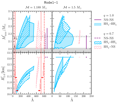
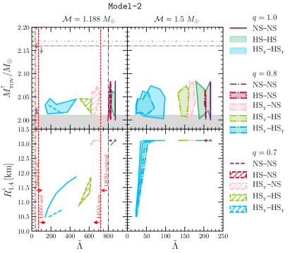
Figure 11: Left plot: Maximum mass (upper panels) and radius of a $1.4\,M_{\odot}$ star (lower panels) as a function of the weighted $\tilde{\Lambda}$ for the same cases as in the left plot of Fig. 10. Right plot: Maximum mass (upper panels) and radius of a $1.4\,M_{\odot}$ star (lower panels) as a function of the weighted $\tilde{\Lambda}$ for the same cases as in the right plot of Fig. 10. In these plots, together with the constraints on tidal deformability, we display a lower horizontal band coming from the lower limit of $2\,M_{\odot}$ observations Demorest et al. (2010); Antoniadis et al. (2013) as well as recent constraints on the maximum mass of $\sim 2.16$–$2.17\,M_{\odot}$ from multi-messenger observations of GW170817 Margalit and Metzger (2017); Rezzolla et al. (2018).

The properties of the phase transition, which are contained in the two free parameters $\Delta e$ and $p_{\rm tr}$, can be constrained using the observational information on tidal deformabilities of the GW170817 event. Moreover, given an allowed space of parameters for $\Delta e$ and $p_{\rm tr}$, the predictions for the maximum mass and the reference radius $R_{1.4}$ can be further restricted by taking into account the limits set on the maximum mass and reference radius after the detection of GW170817.

In what follows we discuss how to constrain twin-star models with GW170817 and we start by studying the values of $\Delta e$ and $p_{\rm tr}$ as a function of $\tilde{\Lambda}$.

Figure 10 reports the ranges in $\Delta e$ and $p_{\rm tr}$ for the Model-1 (left plot) and Model-2 (right plot) EOSs yielding twin stars of Category III, as a function of $\tilde{\Lambda}$ for a chirp mass $\mathcal{M}=1.188\,M_{\odot}$ (left panels of each plot). In addition, we also show results for a higher chirp mass of $\mathcal{M}=1.5\,M_{\odot}$ (right panels of each plot), so as to have access to larger $M_{1}$ and $M_{2}$ masses closer to the $2\,M_{\odot}$ limit.

For the Model-1 EOSs, in particular, we use two different values of the mass ratio $q:=M_{2}/M_{1}=0.7$ (i.e., $M_{1}=1.64\,M_{\odot}$, $M_{2}=1.14\,M_{\odot}$ for $\mathcal{M}=1.188\,M_{\odot}$, and $M_{1}=2.07\,M_{\odot}$, $M_{2}=1.45\,M_{\odot}$ for $\mathcal{M}=1.5\,M_{\odot}$) and $q=1$ (i.e., $M_{1}=M_{2}=1.36\,M_{\odot}$ for $\mathcal{M}=1.188\,M_{\odot}$ and $M_{1}=M_{2}=1.72\,M_{\odot}$ for $\mathcal{M}=1.5\,M_{\odot}$), which correspond to the constraints set by the analysis of the LIGO/Virgo data in Refs. Abbott et al. (2017); Tews et al. (2018a). For the Model-2 EOSs, instead, we use $q=0.7,1$ for $\mathcal{M}=1.188\,M_{\odot}$, whereas we take $q=0.8,1$ for $\mathcal{M}=1.5\,M_{\odot}$ (note that a maximum mass of $2\,M_{\odot}$ is reached easier for a Model-1 EOS than for a Model-2 EOS, as seen in Fig. 4). This is due to the presence of the Gibbs mixed phase that softens the EOS for the transition region (by contrast, the Maxwell construction leads to the stiffest EOS parametrization in the quark phase). By increasing $q$ to $0.8$, we have access to a value of $M_{1}=1.93\,M_{\odot}$, slightly below $2\,M_{\odot}$ and thus easier to be found within Model-2. In the case of $\mathcal{M}=1.188\,M_{\odot}$, we also show with vertical lines the LIGO/Virgo upper limit of $\tilde{\Lambda}=800$ Abbott et al. (2017), as well as the improved analysis of Ref. Abbott et al. (2019), which gives of $70<\tilde{\Lambda}<720$. We also show the lowest value of $\Lambda_{1.4}$ for a star with a phase transition, i.e., $\Lambda_{1.4}>35.5$ (at $2$-$\sigma$ level) of Ref. Most et al. (2018a). We note that our results are overall consistent with the previous results of Refs. Tews et al. (2018a); Han and Steiner (2018); Zhao and Lattimer (2018).

In summary, Fig. 10 shows that, in agreement with the results reported in Refs. Paschalidis et al. (2018); Alvarez-Castillo et al. (2018); Christian et al. (2019), a HQPT softens the EOS and expands the parameter space of EOSs that are compatible with the GW170817 event, allowing for HS${}_{{}_{\rm T}}$–HS${}_{{}_{\rm T}}$ configurations, while HS${}_{{}_{\rm T}}$–NS solutions for $q=0.7$ are also permitted. Such constraints also allow for HS${}_{{}_{\rm T}}$–HS configurations at $q=0.7$ for a Model-2 EOS. The global parameters of the HQPT ($p_{\rm tr}$ and $\Delta e$) are thus constrained by GW170817 to be in the range

$$\bullet\texttt{Model-1}$$

$$\quad p_{\rm tr}\in[25,65]\,\rm MeV\,fm^{-3}, \Delta e\in[175,395]\,\rm MeV\,fm^{-3}\,,$$

$$\bullet\texttt{Model-2}$$

$$\quad p_{\rm tr}\in[15,45]\,\rm MeV\,fm^{-3}, \Delta e\in[380,435]\,\rm MeV\,fm^{-3}\,.$$

Note that for a larger $\mathcal{M}=1.5\,M_{\odot}$, a larger range of $\Delta e$ and $p_{\rm tr}$ parameters is found for both models, with lower values of $\tilde{\Lambda}$ up to $\sim 220$; since these specific values correspond to the NS–NS configuration, they obviously depend on the specific hadronic EOS considered.

In a similar manner, the plots of Fig. 11 display the maximum mass (upper panels) and minimum radius for a $1.4\,M_{\odot}$ star (lower panels) for the Model-1 (left plot) and Model-2 (right plot) EOSs as a function of $\tilde{\Lambda}$ for the same NS and HS/HS${}_{{}_{\rm T}}$ configurations and at the same mass ratios in the plots of Fig. 10. Note that as in Fig. 10, the left panels for each plot in Fig. 11 refer to $\mathcal{M}=1.188\,M_{\odot}$, while the right ones to $\mathcal{M}=1.5\,M_{\odot}$.

Together with the previous constraints on the tidal deformability shown in Fig. 10, we display in Fig. 11 the excluded range of masses up to the $2\,M_{\odot}$ limit coming from $2\,M_{\odot}$ observations Demorest et al. (2010); Antoniadis et al. (2013); Arzoumanian et al. (2018), as well as recent constraints on the maximum mass of $\sim 2.16$–$2.17\,M_{\odot}$ from multi-messenger observations of GW170817 Margalit and Metzger (2017); Rezzolla et al. (2018). We note that for the Model-2 EOSs, and $q=0.7$ and $\mathcal{M}=1.188\,M_{\odot}$, the HS${}_{{}_{\rm T}}$–HS${}_{{}_{\rm T}}$, HS${}_{{}_{\rm T}}$–HS and HS${}_{{}_{\rm T}}$–NS configurations satisfy the maximum-mass constraints for the whole range of values of $\Delta e$ and $p_{\rm tr}$. On the other hand, for the Model-1 EOSs (again with $q=0.7$ and $\mathcal{M}=1.188\,M_{\odot}$), the HS${}_{{}_{\rm T}}$–HS${}_{{}_{\rm T}}$ and HS${}_{{}_{\rm T}}$–NS solutions satisfy the constraint for less than $~{}50\%$ of the parameter space, further requiring the energy-density jump to be $\Delta e\in[245,395]\rm\,MeV\,fm^{-3}$. This is due to the fact that the maximum mass increases as $\Delta e$ decreases, as long as $p_{\rm tr}$ is not too high (see also Fig. 2 of Alford et al. (2015)). As a result, imposing a $M_{{}_{\rm TOV}}^{{}^{\uparrow}}<2.16-2.17$ rules out small $\Delta e$ values. A similar behaviour for a $\mathcal{M}=1.5\,M_{\odot}$ is seen, although in this case we cannot impose any constraint on $\tilde{\Lambda}$.

Reference				$R_{i}\,{\rm[km]}$
Without a phase transition
Bauswein et al. Bauswein et al. (2017)			$10.68^{+0.15}_{-0.03}\leq$	$R_{1.6}$
Most et al. Most et al. (2018a)			$12.00\leq$	$R_{1.4}$	$\leq 13.45$
Burgio et al. Burgio et al. (2018)			$11.8\leq$	$R_{1.5}$	$\leq 13.1$
Tews et al. Tews et al. (2018a)			$11.3\leq$	$R_{1.4}$	$\leq 13.6$
De et al. De et al. (2018)			$8.9\leq$	$R_{1.4}$	$\leq 13.2$
LIGO/Virgo Abbott et al. (2018)			$10.5\leq$	$R_{1.4}$	$\leq 13.3$
Koeppel et al. Köppel et al. (2019)			$10.9\leq$	$R_{1.4}$
With a phase transition
Annala et al. Annala et al. (2018)				$R_{1.4}$	$\leq 13.6$
Most et al. Most et al. (2018a)			$8.53\leq$	$R_{1.4}$	$\leq 13.74$
Burgio et al. Burgio et al. (2018)				$R_{1.5}$	$=10.7$
Tews et al. Tews et al. (2018a)			$9.0\leq$	$R_{1.4}$	$\leq 13.6$
This work
NS				$R_{1.4}$	$=13.11$
HS	Model-2		$12.9\leq$	$R_{1.4}$	$\leq 13.11$
HS${}_{{}_{\rm T}}\ \ \$	Model-1		$10.1\leq$	$R_{1.4}$	$\leq 12.9$
HS${}_{{}_{\rm T}}\ \ \$	Model-2		$10.4\leq$	$R_{1.4}$	$\leq 11.9$

Table 2: Constraints on the radius of neutron stars from GW170817 for models without a phase transition (top), works considering the possibility of a transition to quark matter (middle) and for EOSs of Category III in the present work (bottom).

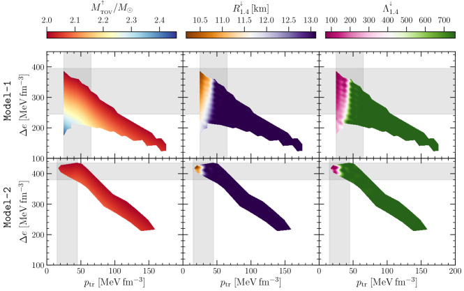
Figure 12: Maximum mass (left panels), minimum radius of a $1.4\,M_{\odot}$ star (middle panels) and minimum tidal deformability of a $1.4\,M_{\odot}$ star (right panels) as a function of the values of the transition pressure and energy-density jump of twin stars of Category III for the Model-1 (upper panels) and Model-2 (lower panels) EOSs. The shaded areas correspond to the parameter space allowed by the GW170817 constraints on ${\Lambda}_{1.4}^{{}^{\downarrow}}$ and $M_{{}_{\rm TOV}}^{{}^{\uparrow}}$ (see details in the text).

As for the limits on the radius of $1.4\,M_{\odot}$, several works have reported values for stars of a given mass Annala et al. (2018); Most et al. (2018a); Abbott et al. (2018); De et al. (2018); Tews et al. (2018a); Kumar et al. (2018); Fattoyev et al. (2018); Malik et al. (2018); Lim and Holt (2018); Raithel et al. (2018); Burgio et al. (2018) and we have collected them in Table 2. Also, we recall that in Ref. Sieniawska et al. (2018) it was found that the minimal radius that can be produced on a twin branch lies between $9.5$ and $10.5\,{\rm km}$. This result was obtained using a set of relativistic polytropes and a quark bag model for the phase transition with a Maxwell construction.

When concentrating on the predictions of this work, and obviously for the hadronic EOS considered here, we note that for the allowed configurations of type HS${}_{{}_{\rm T}}$–HS${}_{{}_{\rm T}}$ and HS${}_{{}_{\rm T}}$–NS with mass ratio $q=0.7$ and for the Model-1 and Model-2 EOSs, we find that $10<R_{1.4}/{\rm km}\lesssim 13$ and that $10<R_{1.4}/{\rm km}\lesssim 12.5$ when considering only HS${}_{{}_{\rm T}}$–HS${}_{{}_{\rm T}}$ solutions. Similarly good agreements with previous investigations can be found when considering HS${}_{{}_{\rm T}}$–HS binaries with $q=0.7$ and the Model-2 EOSs. On the other hand, larger radii closer to $13\,{\rm km}$ are reached when $\mathcal{M}=1.5\,M_{\odot}$ for HS${}_{{}_{\rm T}}$–HS${}_{{}_{\rm T}}$ configurations for both Model-1 and Model-2 EOSs.

A summary plot of our results is given in Fig. 12, where we show the maximum mass, $M_{{}_{\rm TOV}}^{{}^{\uparrow}}$, the minimum radius of a $1.4\,M_{\odot}$ star, $R_{1.4}^{{}^{\downarrow}}$ , and the minimum tidal deformability for the same star, $\Lambda_{1.4}^{{}^{\downarrow}}$, as a function of the values of the transition pressure and energy density of twin stars of Category III for the Model-1 (upper panels) and Model-2 EOSs (lower panels). With shaded areas we indicate the parameter space allowed by the GW170817 as analysed in Fig. 10; once again, the value of $R_{1.4}$ relative to NSs depends on the hadronic EOS considered here.

Overall, we find that $M_{{}_{\rm TOV}}^{{}^{\uparrow}}\simeq 2$–$2.1\,M_{\odot}$ are commonly generated for both models, whereas $R_{1.4}^{{}^{\downarrow}}\simeq 13\,{\rm km}$ and $\Lambda_{1.4}^{{}^{\downarrow}}\simeq 700$ are also produced for almost the entire range in the $(p_{\rm tr},\Delta e)$ space. The lowest values of $R_{1.4}^{{}^{\downarrow}}\simeq 10\,{\rm km}$ and $\Lambda_{1.4}^{{}^{\downarrow}}\simeq 100$ are produced for transition pressures well below $p_{\rm tr}=50\,{\rm MeV\,fm^{-3}}$, i.e., $\rho_{\rm tr}=2.4\,\rho_{0}$. If such small radii and tidal deformabilities given by our hadronic EOS are confirmed by future measurements, the HQPT with a Maxwell construction would imply that hyperons exist in a very narrow region of the interiors of neutron stars. In the case of the FSU2H model Tolos et al. (2017a, b), only the $\Lambda$ particle would be present, since it appears at $\rho=2.2\,\rho_{0}$ (see Fig. 2). In the case of a Gibbs construction of the HQPT, hyperons would still exist in the mixed phase before entering the pure deconfined quark phase and the fractions of these particles would depend on both the hadronic and quark models at these densities. Hence, if future detections of gravitational waves from LIGO/Virgo determine values of $\Lambda_{1.4}\lesssim 400$ and, at the same time, chirp masses $\mathcal{M}\lesssim 1.2M_{\odot}$, our modeling reveals that these can be interpreted in terms of a HQPT with a low transition pressure taking place during the inspiral. Otherwise, it will be difficult to distinguish during the inspiral whether one of the components of the binary is a HS, as a HQPT with transition pressures above $50\,{\rm MeV\,fm^{-3}}$ might be indistinguishable from no phase transition.

IV Conclusions and Outlook

We have performed an extensive and detailed analysis of the features of the hadron-quark phase transition that is needed in order to obtain twin-star configurations and enforcing, at the same time, the constraint on the minimum value of the maximum mass, i.e., $M_{{}_{\rm TOV}}\gtrsim 2\,M_{\odot}$ and the information on multi-messenger observation of the GW170817 event. In our analysis we have employed two general EOS models for the neutron-star matter, i.e., Model-1 and Model-2 EOSs, that share the same description for the hadronic EOS, but take into account a parametrization of the hadron–quark phase transition assuming either a Maxwell or a Gibbs construction, combined with a constant speed of sound (CSS) parametrization for the quark phase.

The parameter space of the phase transition, which is set by the energy-density jump and transition pressure, $\Delta e$ and $p_{\rm tr}$, has been explored systematically and the twin-star solutions found have been classified according to Categories I-IV Christian et al. (2018). We find that the largest number of twin-star solutions that satisfy the $2\,M_{\odot}$ constraint is Category III, with masses in the normal-neutron-star branch of $1$–$2\,M_{\odot}$ and maximum masses of the twin-star branch $M_{{}_{\rm TOV,T}}\gtrsim$ $2\,M_{\odot}$. This category is potentially the most interesting one, as it accommodates twin stars with masses around the canonical value of $1.4\,M_{\odot}$. The masses, radii and tidal deformabilities have been thoroughly studied for the different categories and parameter sets, showing that, when twin-star solutions appear, the tidal deformability also displays two distinct branches having the same mass. This behaviour, which is in agreement with what is found in Refs. Burgio et al. (2018); Sieniawska et al. (2018); Christian et al. (2019), is radically different from what is shown for pure neutron stars and could be used as a signature for the existence of twin stars.

Making use of the large space of solutions found, we have considered the evidence for the existence of EOSs with a HQPT and thus originating twin-star solutions. In particular, we have exploited the weighted tidal deformability and chirp mass, as deduced from the recent binary neutron-star merger event GW170817. In this way, we have found that the presence of a phase transition is not excluded by the observational data and that, in addition to standard NS–NS binaries, also binaries of the type HS${}_{{}_{\rm T}}$–HS${}_{{}_{\rm T}}$ and HS${}_{{}_{\rm T}}$–NS (for Model-1 and Model-2 EOSs) and HS${}_{{}_{\rm T}}$–HS (for Model-2 EOSs) are allowed, in principle. In addition, we have used the multi-messenger astronomical observations associated with GW170817, namely, the new predictions on the maximum mass, to set constraints on the values of $\Delta e$ and $p_{\rm tr}$, as well as on the radius of a reference model with a mass of $1.4\,M_{\odot}$.

Interestingly, the time of occurrence of the HQPT in a binary system of compact stars will depend on the total mass of the binary and on the global properties of the HQPT (i.e., $\Delta e$ and $p_{\rm tr}$). For example, in the case of a binary with chirp mass $\mathcal{M}=1.188~{}M_{\odot}$ (as for GW170817), and assuming that the hadronic part of the EOS is given by the FSU2H model Tolos et al. (2017a, b), the phase transition takes place (at least for one of the two stars) already in the inspiral phase. In particular, the lower the transition pressure, the lower the minimum chirp mass for the HQPT to occur in pre-merger NSs. The lowest chirp mass leading to the appearance of a phase transition is $0.6\,M_{\odot}$ and, quite generically, higher chirp masses are needed in the equal-mass case to obtain a phase transition. Indeed, our results show that future gravitational-wave detections with chirp masses $\mathcal{M}\lesssim 1.2M_{\odot}$ and, at the same time, tidal deformabilities of $\Lambda_{1.4}\lesssim 400$, can be interpreted as due to a HQPT with a low transition pressure taking place in the inspiral phase. Because these precise values depend on the chosen hadronic EOS, we have also considered the hadronic FSU2 model, which represents the baseline of the FSU2H model employed in this work and is stiffer around saturation density, giving rise to higher values of $R_{1.4}$ and $\Lambda_{1.4}$ for the hadronic phase. At the same time, because of the similar stiffness at high densities, the values of the $\Lambda_{1.4}$ and chirp mass where the phase transition takes place are similar to both models as well as the twin-star parameter space. The dependence of our results on the chosen hadronic EOS will be the subject of our future work.

On the other hand, if the central pressure of either of the two stars is below $p_{\rm tr}$ during the inspiral, then a measurement of the tidal deformabilities cannot contain information on the properties of the structure of the HQPT. For such cases, the HQPT will take place during the post-merger evolution of the merger remnant, giving rise to a variety of interesting phenomena. For instance, the rearrangement of the angular momentum in the remnant as a result of the formation of a quark-core could be accompanied by a prompt burst of neutrinos followed by a gamma-ray burst Cheng and Dai (1996); Bombaci and Datta (2000); Mishustin et al. (2003). Furthermore, the $f_{2}$-frequency peak of the gravitational-wave signal Takami et al. (2014, 2015); Rezzolla and Takami (2016) would change rapidly due to the sudden speed up of the differentially rotating remnant Hanauske et al. (2018); Hanauske and Bovard (2018).

Preliminary investigations in this direction have already been made and the consequences of the appearance of the HQPT after the merger and its impact on the spectral properties of the emitted gravitational waves have been recently discussed in Refs. Most et al. (2018b); Bauswein et al. (2018). Although the two studies have employed different temperature-dependent EOSs which include a strong HQPT but do not allow for twin-star solutions, both reach the conclusion that the impact of the phase transition might be measurable with future gravitational-wave detections Most et al. (2018b); Bauswein et al. (2018). Such measurement, together with those performed by X- and gamma-ray space missions such as NICER Arzoumanian et al. (2014), eXTP Watts et al. (2019) and THESEUS Amati et al. (2018), have the potential of providing essential information to clarify whether a HQPT should indeed be accounted for a binary neutron-star merger.