Abstract

The structure of defect clusters formed in a displacement cascade plays a significant role in the micro-structural evolution during irradiation. Molecular dynamics simulations have been widely used to study collision cascades and subsequent clustering of defects. We present a novel method to pattern match and classify defect clusters. A cluster is characterized by the geometrical and topological histograms of its angles and distances which can then be used as similarity metrics. The technique is demonstrated by matching similar clusters for different cluster shapes like ring, crowdions etc. in a database of cascade damage configurations in Fe and W at different energies. We further use graph based dimensionality reduction techniques and unsupervised machine learning on the features of all the clusters present in the database to find classes of clusters. The classification successfully separates out many already known categories of clusters such as crowdions, planar crowdion pairs, rings and perpendicular crowdions. The dimensionality and size of different classes provides a broad categorization of classes. The distribution of different classes of shapes among cascades of different elements and energies shows the exclusivity of shapes to elements and energies. We discuss the key points and computational efficiency of the algorithms along with the various prominent results of their application. We discuss the motivation for using machine learning and statistics for the problems and compare different techniques. The algorithms along with the supporting analysis and visualizations give an unsupervised approach for classification and study of defect clusters in cascades. The distribution of cluster shapes and structures along with the shape properties like diffusivity, stability, etc. can be used as input to higher scale models in a multi-scale radiation damage study.

1 Introduction

The defects formed during the displacement cascades due to irradiation are the primary source of radiation damage [1, 2, 3, 4, 5, 6, 7]. The defects in metals with body-centered cubic structure are produced in the form of single point defects (interstitials and vacancies) or clusters of such defects. The point defects and glissile clusters diffuse after the cascade to either annihilate or form bigger defect clusters. The structural details of primary point defect clusters (formed as a direct consequence of the cascade) define the diffusion, recombination, thermal stability and their other characteristics [2, 8, 9, 10] which in the long term determine the micro-structural changes in the material [11, 12, 13, 14, 15]. These properties have an affect on the results of higher scale models like Monte Carlo methods, rate theories etc. [13, 14, 7, 16]. The glissile clusters can move and interact with other defects and grain boundaries whereas the sessile clusters can be nucleation centers for defect-growth. The interaction of these clusters with other defects will decide the micro-structural changes due to irradiation. Classification and taxonomy of all possible clusters in different irradiated samples is the first step in the systematic study of properties of clusters and their effects.

We approach the problem of characterization, matching and classification of point defect clusters using the techniques of topology, geometric shape pattern matching, statistics and unsupervised machine learning. A cluster is characterized by the normalized histogram of angles between the neighbouring defect triads and pair wise distances. We use this histogram as a feature vector for the cluster. To find the similarity between two clusters it is sufficient to find the distance between the two feature vectors that represent them. The histograms of angles, distances and adjacency are a simple, deformation invariant, computationally efficient but powerful way to characterize a shape [17]. Other advanced topological techniques such as barcode like representation from simplices [18] can also be effective. We further use topological network graph based dimensionality reduction techniques on the feature vectors. The network graph based dimensionality reduction techniques are well established ways to find a representation in the reduced dimensional space such that the distance between the distinct points is maximized [19, 20] and similar points are represented closely. The reduced dimensional representation is also known as embedding of the feature representation. We then use an unsupervised clustering algorithm to classify the clusters without any inputs and assumptions made. With the help of classification we can explore the dimensionality, sizes and exclusivity of certain shapes in elements and energy ranges. Some classes of clusters we found in Fe have been reported in [21].

We present the results on a database of cascade damage configurations simulated by molecular dynamics (MD) [22, 23]. The database has Fe and W cascades at different energies ranging from 10 keV to 200 keV. The code is integrated with interactive visualizations built using webGL interface making it easy to qualitatively study and understand the results.

Section 2 describes the various algorithms and methods used in every step with a brief discussion on the suitability of the method used to solve the problem and comparison with related techniques. The implementation of the methods along with interactive web-app can be found at https://github.com/haptork/csaransh open source repository. Section 3 presents results of the faster defects identification algorithm implementation, pattern matching and searching of similar clusters in the database, dimensionality reduction and classification of clusters for the database. The results for the database can be accessed via interactive web application available at https://haptork.github.io/csaransh. Finally, we conclude by discussing the significance of using the presented method for the study of radiation damage.

2 Algorithms and Methods

The problems of classification and pattern matching find state-of-the-art solutions in machine learning and artificial intelligence. After finding the defect clusters, we divide the problem of characterization, matching and classification of clusters into the following machine learning template steps:

1. Feature representation

2. Dimensionality reduction

3. Classification with an unsupervised clustering algorithm

In the feature representation step, we find a representation of a cluster that approximately characterizes its shape and ensures translational, scale and rotational invariance. The distance between the two feature representations can be used as the (dis-)similarity metric of their clusters. The next step viz. dimensionality reduction, transforms the feature space into a space with reduced principle dimensions. The network graph based dimensionality reduction approaches that we employ aim to increase the probability that similar points appear nearer and dissimilar points have distant embedding (feature vector in new space). By reducing to two or three dimensional space we can qualitatively check the global and local relationships between all the clusters and also explore how the embeddings separate out known groups like interstitials and vacancy clusters, different sizes etc. Next, we use the embeddings for classification using unsupervised clustering. We use density based clustering algorithms, that group together the points (here, cluster embeddings) that are densely packed together and ignore the noise. We then explore different statistical properties of the classes like dimensionality, size and specificity of shapes among different elements and energies.

Starting from how we find the defects and clusters from MD simulation output to classification, we provide a detailed description of each step in the following sub-sections.

2.1 Finding Defects and Clusters from MD simulations

To find the defects from all the atoms in the last frame of an MD simulation, we use an algorithm that is similar to Wigner-Seitz method [24, 25], but more efficient and also finds extra interstitial-vacancy pairs crucial to defining shape of the cluster e.g. a crowdion cluster can be formed of three interstitials and two vacancies; although the defect count is one interstitial but the shape and dependent properties are a function of all the five defects.

The algorithm can be divided into two stages. The first stage is to assign closest lattice site to every atomic coordinate that is achieved by using the modulo arithmetic [26]. The steps are as follows:

• For every atom:

  1. Find the modular position by taking modulo (remainder) of coordinate values by lattice constant. This gives the position of the atom within a unit cell.

  2. Using the modular position, find the minimum distance lattice site position in the first unit-cell out of all the lattice sites possible for the given lattice structure (bcc, fcc etc.).

  3. Find the unit cell in which the atom lies by taking quotient of coordinate values by lattice constant.

  4. Using the closest lattice site in the first unit cell found in the second step and the unit cell in which the atom lies found in the third step, assign the closest lattice site position to the atom.

The algorithm can run in parallel for all the atoms. The implementation utilizes the crystal structure information to calculate the closest lattice site using modulo arithmetic. The other implementations that use the initial atomic coordinates as template require extra memory to store the template structure. They either require simple but slow $\mathcal{O}(N^{2})$ look-up or need to build a special datastructure for nearest neighbour search such as k-d tree that is $\mathcal{O}(kNlogN)$ to build and $\mathcal{O}(NlogN)$ for the look-up of neighbours for all the N atoms. Our implementation takes only single pass through the data making the operation $\mathcal{O}(N)$. It is also completely parallelizable. Since it is just a single, continuous pass through the data, it gives good cache performance. However, a template free approach is only possible for the crystal lattices, where points can be enumerated and one to one mapping can be implemented between the enumeration and the lattice site coordinates in the crystal. In the stage two we make use of the mapping to go from index of a lattice site to the atomic coordinates and vice-verse. The steps are as follows:

1. Initialize a boolean array with false values having size same as total number of atomic sites.

2. Iterate over the array of atomic coordinates:

   1. Check the value of the boolean array at index equals to the closest site lattice enumeration added for the current atomic coordinate in stage 1.

   2. If the value is false, mark it as true.

   3. Else (if the value is true, implying there was another co-ordinate that had this index as closest lattice site), mark the current atomic coordinate as interstitial.

3. Iterate over the boolean array and mark all the indices (or the coordinates corresponding to the indices) that hold false value (implying that no atom had these indices as closest lattice site) as vacancy.

To make the algorithm output extra interstitial-vacancy pairs, we can change the algorithm such that in the case where the value at index in the boolean array is already true, mark not just the current atom as interstitial, but also mark as interstitial the first atom that made the boolean array value true and the lattice site for the index as vacancy. We can keep an extra flag to mark these as pseudo defects.

Unlike template based Wigner-Seitz or similar methods, the algorithm never holds the whole perfect lattice in memory and does not require neighbour search, runs faster with $\mathcal{O}(N)$ time-complexity and uses simpler cache-friendly datastructures.

The machine learning method described in [26, 27] that uses max-space clustering on offsets of atoms, has $\mathcal{O}(NlogN)$ time-complexity but probably has faster implementation than k-d tree, requires no lattice or any other information. However, it can only be used to identify interstitials and not the vacancies. The other sphere based methods [2, 28], require a threshold and would also require a neighbour search for finding interstitials and vacancies. The other implementation of the threshold based sphere method as given in [29] requires initial position with atom i.d. to match between initial and final positions of all the atoms.

The algorithm presented in this work takes only final positions and crystal structure as input, makes no extra assumptions and on a single run can output both interstitials, vacancies as well as structural defects that can be separately labelled, e.g. as pseudo-defects. These pseudo-defects do not appear in an analysis based on the use of Wigner-Seitz cells.

To find the clusters from the identified defects, we use distance threshold and union-find [30] data structure to find the clusters efficiently [29]. The extra interstitials and vacancies found by the method also contribute to the clustering so that all the defects in crowdions, complex ring structures etc. are grouped in the same cluster.

2.2 Finding the Feature vector for a cluster

We characterize a cluster by histograms of: angles of triplets, distances between pairs and number of neighbours of the defects in the cluster. The first two features are based on geometry while the last one is based on topology. Following are the algorithms for each.

2.2.1 Histogram of Angles

1. Choose a bin size for the angles between 0 and 180, a reasonable default can be between 3 to 15 degrees.

2. Initialize all the bins with zeroes.

3. For each vacancy in the cluster find the angle that two neighbouring interstitials or two neighbouring vacancies subtend. Find the bin where the angle falls and increase the count of that bin by one.

We find angles only with vacancy as the pivot of the triad and the other two defects are either both interstitials or both vacancies. Since, vacancies are at the fixed lattice points, it is equivalent to measuring the arrangement of interstitials and other vacancies that are around. Adding more angles such as with interstitials as pivot adds no extra information about the shape.

2.2.2 Histogram of Distances

1. Choose a bin size for normalized distances between 0.0 to 1.0, a reasonable default can be between 0.01 to 0.1.

2. Initialize all the bins with zeroes.

3. For each vacancy in the cluster find the distances from its neighbours.

4. Divide all the distances by the maximum distance, to normalize between 0.0 and 1.0.

5. Find the bin where distances fall and for each one increase the count of that bin by one.

Again, we take only the distances from fixed vacancy points, since adding more distances does not further enrich the information.

2.2.3 Histogram of Neighbours

1. Initialize all the bins with zeroes.

2. For each defect in the cluster find the number of neighbours and increment by one the bin at the index equal to number of neighbours.

For each of the above algorithms we use twice of 4-NN (nearest neighbour) as the neighbourhood distance that is similar to considering defects in adjacent unit-cells alone. We use 5 degrees for the angles bin size and 0.02 as the distance bin size for the histogram feature representation. However, the results are not very sensitive to these values.

The histograms accumulate the local geometry of each defect. Since the adjacency histogram captures a subset of details captured by the distance histogram, we drop adjacency features from the further analysis.

There are similar shape histogram features that have been used before to study molecules [17] which involve angles and distances from the center of mass. However, being independent of the center of mass, the features we use are more robust to noise and can characterize local structures better e.g. if there are two structures, one with ring and one with ring and a tail, the centroid based features will be entirely different while the features presented above will have same values for the bins that correspond to the ring, although the latter structure with a tail will have some more additions on the bins characterizing the tail.

The topology feature we use is simple while there is still scope to use more advanced features like barcode like representation as defined in [18]. One can also use Hausdorff distance etc. after getting the defect coordinates of each cluster in their principle axes by singular value decomposition. However, matching with barcodes or direct matching after transformation in principle axes and strict distance measures will not be as efficient as histogram features matching. Also, the direct matching of structures might suffer because of different orientations, slight distortions and other noises such as thermal displacements due to residual heat, different number of total defects in two similar structures etc. Also, the size of clusters if counted with thermally displaced pseudo defects can grow to a few hundred point defects. For these reasons we find the histogram based features simple and efficient for our case as shown in the results section.

For a cluster, we can find other similar clusters by comparing the distance between histograms. We can use different distance metrics such as chi-square, correlation, Quadratic Form Distance Functions [31]. The definitions of these metrics can be different, however they all consider each bin of the histogram as a dimension. The euclidean distance between two $n$ dimensional histograms ($a$ and $b$) can be defined as $\sqrt{\Sigma_{i=1}^{n}(a_{i}-b_{i})^{2}}$.

2.3 Dimensionality Reduction of the feature vector

Graph based dimensionality reduction techniques like t-SNE [19] (t-Distributed Stochastic Neighbor Embedding) and UMAP [20] (Uniform Manifold Approximation and Projection) are well established techniques for qualitative analysis of relationships between the data points (here clusters). By transforming the basis vectors such that the probability of similar points to appear together increases, these techniques can help in visualizing and exploring classification and correlation of cluster shapes with other quantities like dimensionality of the clusters, size of the cluster etc. In our case both UMAP and t-SNE give very similar global structure. The degree of local spread produced by UMAP is more amenable to the HDBSCAN (Hierarchical Density-based Spatial Clustering of Applications with Noise) [32, 33] classification algorithm. UMAP is also a more efficient algorithm than t-SNE. However, t-SNE gives a relatively more even spread as shown in the results.

2.4 Classification of all the clusters

To get an idea about the different shapes of defect clusters present in the database and arrange them into classes we use unsupervised clustering. Unsupervised clustering can be used to group together similar data points without any need of already labelled training data. We use density based clustering algorithms viz. DBSCAN (Density-based Spatial Clustering of Applications with Noise) [34] with t-SNE and HDBSCAN with UMAP because HDBSCAN works well with UMAP embeddings and not with t-SNE. Density based algorithms classify separated similarly dense point regions into different classes and less dense isolated points as noise. HDBSCAN has the advantage that it only depends on a single integer parameter as opposed to two in DBSCAN. We can use other popular unsupervised classification algorithms like K-Means but unlike density based algorithms K-Means does not ignore the noise in the data and requires number of classes as user input i.e. a-priori information about the number of distinct cluster classes need to be known. Both the density based algorithms used give very similar classifications as shown in the results section.

3 Results

This section discusses the results of the methods described above applied to a collection of defect configurations from collision cascades in bulk W and Fe. Cascades in W were simulated using the method described in [22], with the interatomic potential by Derlet et al. [35], stiffened by Björkas et al. [36]. Cascades in Fe were simulated with the same method, using the Ackland-Mendelev interatomic potential [37]. All cascades were simulated with an initial temperature at 0 Kelvin, and with electronic stopping applied to atoms with energies above 10 eV [38], and evolved for 40 ps. The database contains total 76 collision cascades out of which, 36 are of W at energies 100 keV, 150 keV, 200 keV and 40 are of Fe at energies 10 keV, 20 keV, 50 keV, 100 keV, 150 keV. The cascades have more than a thousand vacancies and interstitial clusters of various shapes and sizes, providing a varied database to work with. The following subsections discuss the significance and validity of each method using the results found on the database.

3.1 Defects and Clusters from Cascades

The algorithm presented to identify the defects in Section 2.1 can find out the extra interstitial-vacancy pairs crucial for defining the shape of a cluster. Fig. 1 shows a cluster of W cascade at 200 keV with and without these extra interstitial-vacancy pairs. The ring shape of the cluster can only be identified with the extra pairs included.

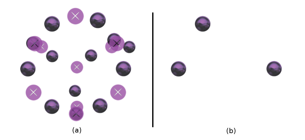
Figure 1: A cluster in W cascade at 200 keV (a) with and (b) without extra displaced atoms and their lattice sites. Solid spheres are interstitials and flat-cross glyph represents vacancies. The ring like shape of the cluster is evident only in (a).

We also validate the accuracy of the algorithm by matching the number of defects against that found with the template based Wigner-Seitz method implemented in Ovito [39]. The results match for all the cascades in the database.

3.2 Feature Vector for a cluster

The histogram features retain the information about the characteristic shape of a cluster that are invariant to rotation, scale etc. while ignoring the superfluous details. Fig. 2 to Fig. 5 show the triad angle histograms next to the cluster shapes for a crowdion, parallel stacked crowdions, ring and two dumbbells arranged in T like structure. The figures show three clusters for each of the shapes. The first cluster is chosen randomly from the database and the other two are its closest neighbours found using the chi-square distance from all the other features of clusters in the database. The histograms when used to search similar clusters in the database place qualitatively similar structures closer to each other than the distinct ones.

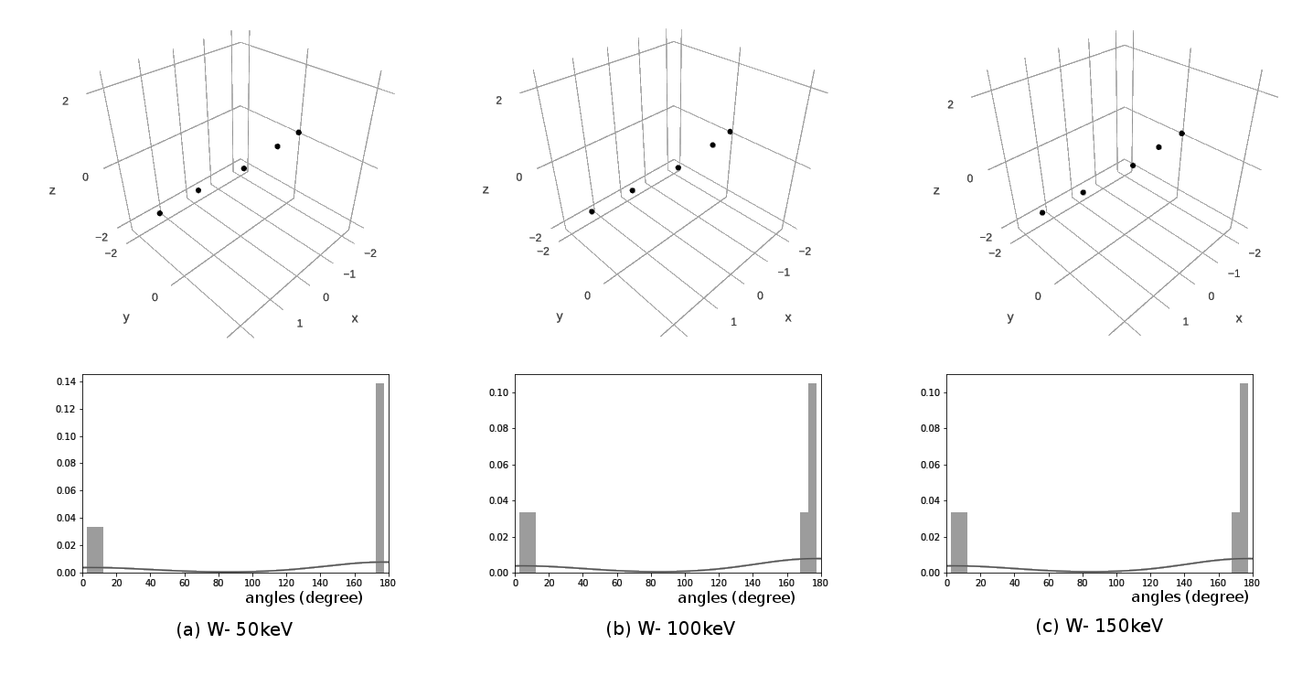
Figure 2: Linear crowdion clusters along with their triad angle histogram feature. The crowdions in (b) and (c) are the results of a search for closest feature to (a) in the database. The histogram shows high number of occurrences in 0 degrees and 180 degrees that is also qualitatively a characteristic for a linear shape.

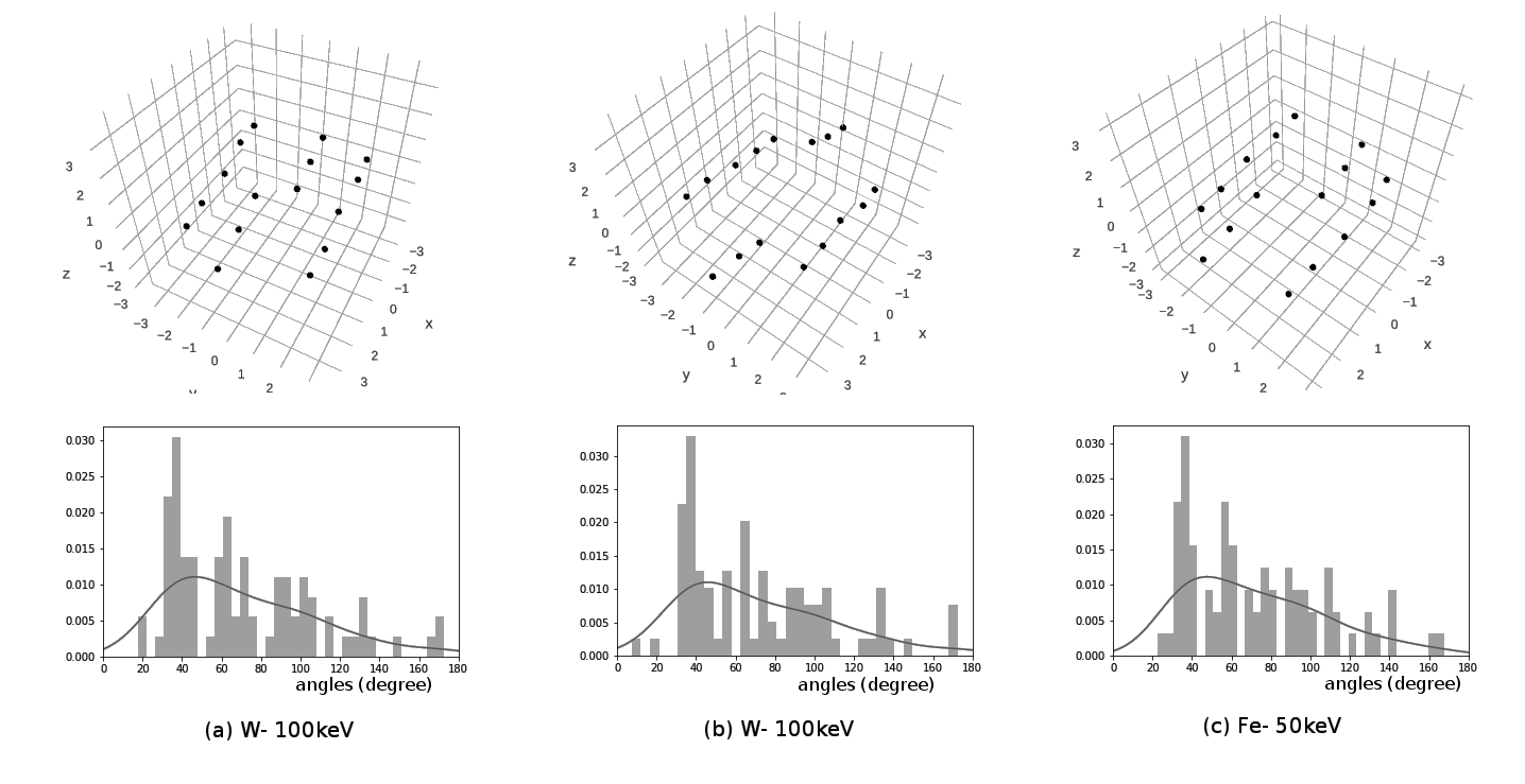
Figure 3: Four stacked crowdions and dumbbells along with their triad angle histogram feature. The clusters in (b) and (c) are the results of a search for closest feature to (a) in the database. The histogram is a characteristic for the shape.

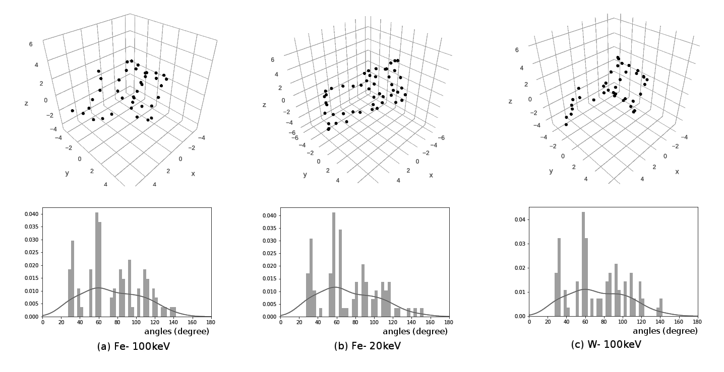
Figure 4: Ring like clusters along with their triad angle histogram feature. The rings in (b) and (c) are the results of a search for closest feature to (a) in the database. The histogram is a characteristic for ring shape.

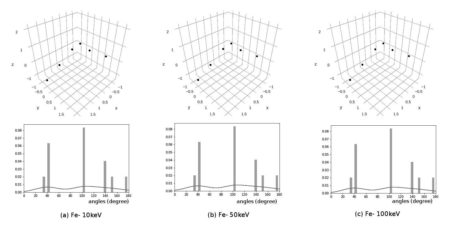
Figure 5: Tee shaped non-planar pair of dumbbells along with their triad angle histogram feature. The rings in (b) and (c) are the results of a search for closest feature to (a) in the database. The histogram is a characteristic for the shape.

The angle histograms for the similar shapes look qualitatively similar and for different shapes look different. In Fig. 3 the cluster in (b) is oriented differently but still the histograms are closely related. Similarly, in Fig. 4 neither the number of defects nor the shapes perfectly match but still the feature representation retains the qualitative similarity of the ring like structure.

In the Fig. 2 the histogram shows high occurrences of angles 0 and 180 degrees which is true for a linear crowdion cluster only. Similarly, other shapes do show characteristic histograms.

3.3 Dimensionality Reduction and Classification

Although the features we found can be used to find similar structures, we need dimensionality reduction to build 2D or 3D plots that can qualitatively show the relationship between the different clusters. Fig. 6 shows the plot of angle and distance features of all the clusters in the database reduced to two dimensional surface using UMAP. Each point in the plot represents a cluster feature. The algorithm tries to maintain the local and global relationship of the shape features. The figure shows that the algorithm embeds vacancy clusters together, separate from interstitial clusters (the term interstitial clusters here and in further discussions implies the clusters that have more interstitials than vacancies). Broadly, the interstitial and vacancy clusters do have different shapes. The embeddings found by the UMAP can change with the change in the parameters that mostly govern the trade-off between local and global structure and distribution of points in space. However, the overall nature of the embeddings remain the same. The embeddings of the t-SNE are also similar with small differences in the details as we show later in this section (Fig. 9).

Figure 6: The UMAP embeddings of the cluster features. The vacancy and interstitial clusters are shown with different colors. The axes represent latent feature space of UMAP transformation.

Fig. 7 shows the classification suggested by the HDBSCAN algorithm. The classes are labelled from zero to twenty-two. The shape and name for each class are also annotated in the figure.

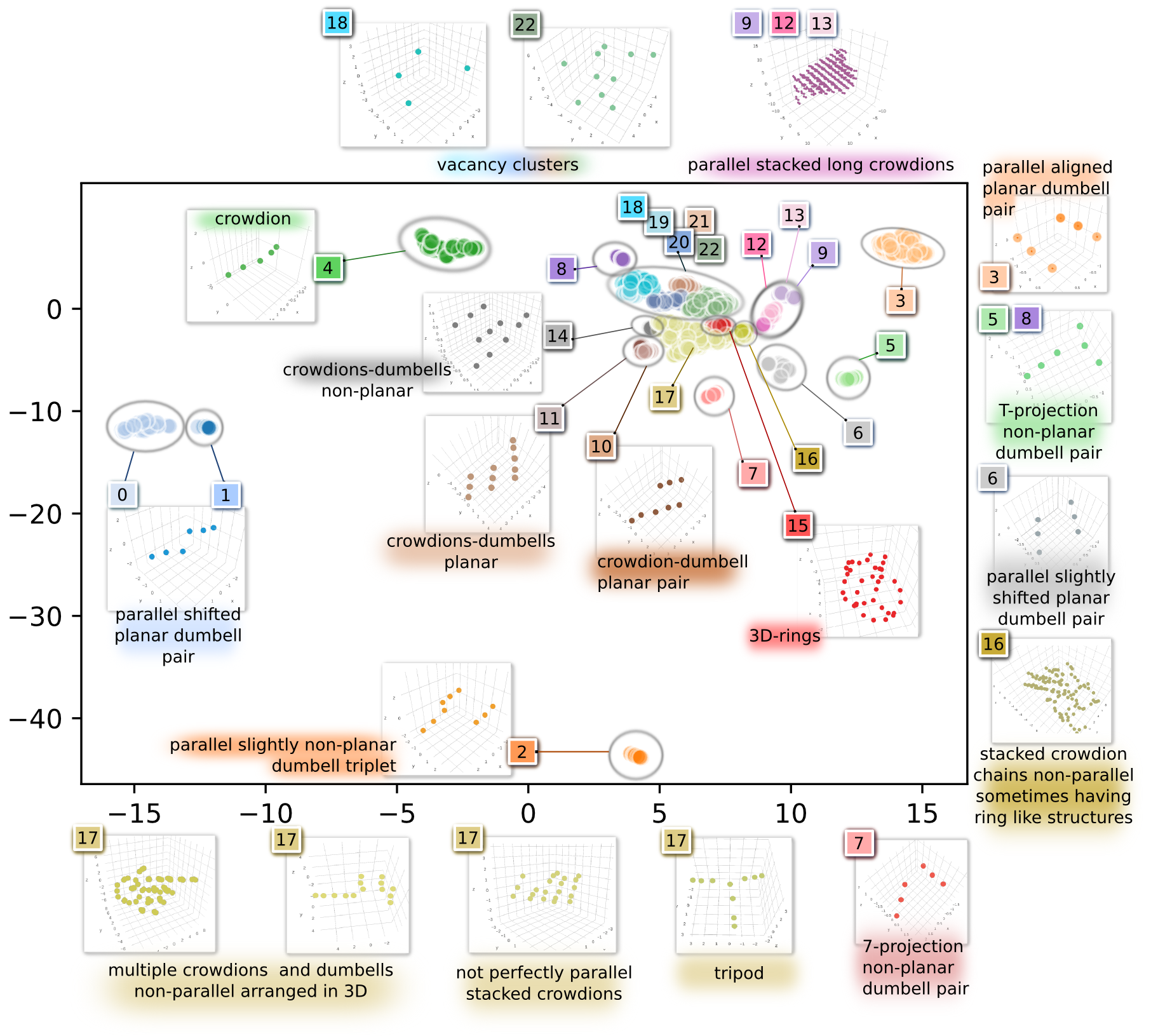
Figure 7: Classification of the clusters using UMAP and HDBSCAN. Different classes are labelled from 0 to 22. The annotations show characteristic shapes for the classes. The axes represent latent feature space of UMAP transformation.

Each class represents shapes of exactly the same type, or closely resembling shapes. In a single class label, the structures can gradually change from one end to the other, e.g. the left end of the 4th class represents perfectly collinear crowdions, while as we move towards the right end (greater value of latent-feature-1) the defects in the crowdions start to look slightly distorted or not perfectly in-line with each other. These ends on zooming in might be seen as sub-classes in a class and by using different values of parameters for the unsupervised classification, might be separated into different classes. The global relationship is also revealed when we move from one class to another. The classes that are close in shape to each other appear close by, e.g. 15th class represents ring-like structures while 16th class, appearing nearby, represents big 3D shapes that have crowdions and dumbbells in random orientations. These can sometimes form partially ring like structures towards the ends. Instead of complete random directions there can be two or more parallel stack of crowdions with different orientations giving an overall appearance of random orientations. Similarly, classes 9th, 13th and 12th show stacked crowdions gradually decreasing in size going from right to left. The trend of decrease in size continues in the 17th class. Indeed, the 17th class has on the periphery structures that look like that of nearby classes and they gradually fade from one structure to the other. The fading of one type of structure into some partially recognizable shape and then finally into a different structure is enticing to see as the structures change size, dimensionality and slowly lose their qualitative characteristic identity. For some of the classes which are totally separate from all others such as 2nd, 4th etc., it is difficult to see the global relationship.

The density based algorithms classify only the similar density classes. Since the structures in 17th class are evenly spaced due to their gradual change and are relatively lesser in number, they are classified into one class. However, if we zoom in, the density clusters can be seen. Fig. 8 shows the sub-classes of 17th class found by applying HDBSCAN to only the points in the class. The sub-classes are named after the classes with which they most relate to. The class 12a is a continuation of long parallel crowdions however shorter than the 12th class. The reduction in size continues in 14a with four or five shorter crowdion chains. The 14th class had only three number of relatively shorter crowdions and dumbbells. The 16a class is just like 16th class but with lesser number of defects and shorter crowdion chains. The 16a class fades into 17c with smaller and more planar randomly oriented dumbbells and crowdions. Similar to 14a and 12a, 17a has three to five crowdions and dumbbells but these are all randomly oriented in a 3D arrangement unlike planar 17c. Sometimes the dumbbells or crowdions share a vacancy to form a characteristic shape. 17b shows a distinct tripod like arrangement of three dumbbells with shared extra defect at top. Sometimes one of the leg of the tripod is missing an interstitial - vacancy pair at the end.

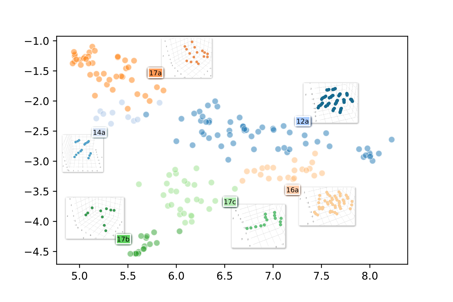
Figure 8: Sub-classification of the clusters in 17th class. The annotations show characteristic shapes for the classes. The axes represent latent feature space of UMAP transformation.

The classification shown in Fig. 7 has a few misclassifications that include assignment of shapes into one class (label 17th) that qualitatively can be divided into different classes and classification of qualitatively similar shapes into two different classes as found in label 5th and 8th, 0th and 1st. While the former case is improved by sub-classification as discussed above, the latter is dealt by the DBSCAN classification on t-SNE embeddings as shown in the Fig. 9. After accounting for these corrections we get 21 classes and 5 sub-classes making a total of 26 classes.

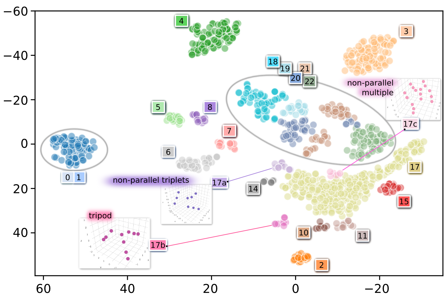
Figure 9: Classification of the clusters using t-SNE and DBSCAN. The class labels are same as Fig. 7. The annotations show characteristic shapes only for the classes that are new in this classification. The axes represent latent feature space of t-SNE transformation.

The t-SNE embeddings also show some sub-classes (17a, 17b, 17c) of the 17th class. The overall shape of the embeddings is very similar to that of UMAP in Fig. 7, however the points are more evenly spaced. The placement of different classes is also very similar e.g. the 4th class of crowdions is at the top, 2nd class at the bottom, 17th class has similar shape and above it are the vacancy classes. However, there are some differences as listed below:

• Classes 0 and 1 that have qualitatively same shape are classified into the same class unlike before.

• Classes 5th and 8th that have qualitatively same shape are placed side by side.

• There are more classes with distinct shapes around 17th class (17a, 17b, 17c) that were also found in the subclassification on UMAP embeddings.

• Classes 9th, 12th and 13th that show gradation of sizes of big stacks of crowdion chains are not classified separate from 17th class. Class 16th is also missing.

3.3.1 Properties of Classification

We now look at the quantitative properties of the clusters present in the various classes. The dimensionality of classes range from one-dimensional crowdions (4th label) to highly planar arrangement of dumbbells and crowdions (0, 1, 3, 11) to 3-D complex structures (15, 16, 16a). The size of classes range from single crowdion (4) to big stacked chains of defects (9) of 1/2(111) loops. The clusters where net defect count gives vacancies are classified into 5 classes from 18 to 22 while all other classes have clusters that have interstitial nature after net defect count.

Fig. 10 shows the dimensionality of the various classes, plotting the point estimates of variances along the principle axes. The principle axes of a cluster are found using the PCA (principle component analysis) using SVD (singular value decomposition). The variance along an axis tells about the spread along that axis. For a linear cluster, all the defects are spread along the first principle axis and the variance along the first principle axis will be 1.0. For a perfectly planar structure points would lie on only two principle axes and the third axis will have no spread making the variance along the first two principle axes 1.0. Thus, The high variance on first principle axis in figure (a) implies a more linear shape. For a non-linear shape, a high variance on first two principle axes, as shown in figure (b), implies a more planar structure. It can be seen that one dimensional crowdions (label 4) are perfectly linear while class labels 0, 1, 3, 10 and 11 are perfectly planar. Classes 2, 6, 7 and 18 are almost planar while 14, 15 and 16 are distinctively 3D structures.

Figure 10: The point estimates of variances as described by (a) first principle axis, (b) first two principle axes together, for different classes. The high value in first implies linearity and for low value in first, high value in second implies more planarity.

Among vacancy cluster classes we see that the 18th class is more planar than any other vacancy cluster class also owing to its very less number of vacancies. The planarity decreases gradually from 19 to 21 while class 22 can be said to be most non-planar again owing to its distinctively big clusters.

Fig. 11 shows the point estimates for total number of defects, including extra vacancy-interstitial pairs, in clusters of each class. Most of the classes have clusters of sizes ten or less while 9th class has really large clusters followed by 13, 12 and 16. The biggest of the vacancy clusters are classified in class 22.

Figure 11: The point estimates of number of total point defects in the clusters assigned to different classes.

Fig. 12 shows the distribution of clusters among classes and cascades of both the elements at each energy of primary knock-on atom with the help of (a) box-plot and (b) heat map with annotated values. Our analysis shows the difference in interstitial cluster morphologies that arises as a result of the different ground state configurations of the interstitial defect, which in W adopts a $\langle 111\rangle$ crowdion configuration (class 4) and in Fe a $\langle 110\rangle$ dumbbell configuration. In addition, the tendency in W to form large defects [22], as opposed to the predominantly small defects in Fe, is quantified in our results. The figure shows some shapes such as those included in classes 3 or 5, 7, 8 and 15 that are exclusive to Fe, while classes 0 or 1, 2, 4, 9 to 14 and 16 that are predominantly present in W. The classes exclusive to W have perfectly parallel stacked crowdion chains of various sizes arranged in different fashion, while in Fe small dumbbells and sometimes longer distorted crowdion like chains are arranged in random orientations, except for class 3 that has a almost perfectly aligned pair of parallel dumbbells. More tendency to form ring like shapes in Fe can also be understood as an extension of this. Some of the classes of clusters obtained in Fe have been reported in [21]. The well investigated 3-D combination of ring like structures in Fe viz. C15 resembles the class 15 structures classified by the unsupervised algorithm. However, a more convincing study to match the different structures found in this work and the earlier reported cluster shapes can be carried out in the future.

Figure 12: The distribution of clusters of different shapes among various elements and energies shown using (a) box-plot, (b) heat map.

Fig. 13 shows the dimensionality, sizes and distribution of clusters in the sub-classes among the elements at each energy. The sizes and dimensionality of the sub-classes is as suggested by their qualitative shape 17b and 17c are almost planar, the size of 12a is less than 12th class and more than 14a which itself has more defects than the 14th class.

Figure 13: Showing the properties of various subclasses of 17th class. The figure (a) and (b) show the point estimates of variances as described by first principle axis and first two principle axes together, respectively. The high value in first implies linearity and for low value in first, high value in second implies more planarity. The figure (c) shows the point estimates of number of total point defects in the clusters assigned to different classes. The heatmap in figure (d) shows distribution of various sub-classes among various elements and energies.

More interestingly, the classes having parallel stacked crowdions and dumbbells viz. 12a, 14a again show up more in W while Fe clusters are predominantly formed of randomly oriented dumbbells appearing in classes viz. 17a, 17c and 16a. However, Fe clusters do appear in classes such as 12a with groups of long but slightly distorted crowdion like chains and W clusters appear in classes like 17a and 17c with randomly oriented distorted (non collinear) dumbbells. The 17b shows a new tripod like arrangement of dumbbells almost exclusive to W.

Broadly the observations and corresponding descriptions of the class labels can be summarized as follows:

1. Linear - specific to W:

   1. Label 4: Crowdions (size 5): Mostly perfectly collinear but sometimes a bit off.

2. Planar:

   1. Dumbbell pairs:

      1. Labels 0, 1: Parallel shifted - specific to W

      2. Label 3: Parallel aligned - specific to Fe

      3. Label 6: Parallel slightly shifted - more common in W

   2. Crowdion-Dumbbells - specific to W:

      1. Label 10: Pair

      2. Label 11: Multiple

   3. Vacancy clusters: Label 18

3. Small, slightly non-planar structures:

   • Label 2: parallel dumbbell triplet - specific to W

   • Labels 5, 8: T-projection dumbbell pair - specific to Fe

   • Label 7: 7-projection dumbbell pair - specific to Fe. This class also has some twisted dumbbell pairs that only partially resemble the structure shown in Fig. 7.

   • Label 17b: crowdion dumbbell triplets - specific to W

   • Label 17c: multiple crowdions and dumbbells - more in Fe

   • Labels 19, 20, 21 Vacancy clusters.

4. Small 3D structures

   • Label 14, 14a: parallel crowdions-dumbbells - specific to W.

   • Label 15: Ring like 3D-shapes - More common in Fe.

   • Label 17a: small number (3 to 5) of randomly oriented dumbbells and crowdions, more in Fe.

5. Bigger 3D shapes - more common in high energies

   • Label 16, 16a: dumbbells and crowdion like chains in different orientations sometimes having ring like arrangements at the ends.

   • Labels 9, 12, 12a, 13: parallel stacked crowdion chains - 9 (biggest), 13 (bigger), 12 (smaller), 12a (smallest).

   • Label

   • Label 22: Big vacancy clusters.

The results shown can be used to characterize and study the class of clusters in new data of collision cascades. The UMAP or t-SNE embeddings can be found for a new defect cluster and then the cluster can be assigned to one of the already found classes based on its proximity. We can also find the statistical distribution of occurrence of classes of defects produced for any element in an energy range from the collision cascades simulation data which can then be used along with the properties like diffusion profile, recombination criteria, stability etc. for the shapes, in higher scale models like Monte Carlo methods, production bias model etc. These properties are known for some of the shapes while for others these need to be explored.

4 Conclusion

We have described a method to efficiently process and analyze the structures of clusters from MD simulations of collision cascades. We have discussed efficient algorithms starting from identification and clustering of defects, to feature engineering for cluster shapes, to their classification and visualization. We use well established approximate algorithms from machine learning that enable a solution with minimum inputs or assumptions and high robustness to noise. The results can be used to study and add shape and structure based information of defect clusters to higher scale models of radiation damage.

We have applied our methods and discussed elaborate results for collision cascades in Fe and W for a wide range of PKA energies. We show that the features we introduce work well for the pattern matching of defect clusters. The dimensionality reduction algorithm helps visualize the relationships between the clusters such as type of clusters (interstitial or vacancy), size of the cluster and dimensionality of the cluster. The unsupervised classification algorithms give twenty six classes that we identify by different qualitative names based on the shapes they represent. The classification can be used to quickly study the kind of clusters produced in new elements and energy ranges. The classification and taxonomy also helps to systematically study and explore the nature of defects caused by collision cascades in different elements and energy ranges and use the properties for that shape in higher scale models in a multi-scale radiation damage study. A next step in a multi-scale model can be to assign the properties such as diffusivity, recombination, thermal stability etc. to the identified classes. While for some cluster structures found, the diffusion profile (sessile or glissile, dimensionality of diffusion, diffusion coefficient etc.) is known, for others it needs to be examined. The interaction of the clusters with other defects and grain boundaries affects the micro-structural changes due to irradiation.

We have laid out the steps that lead to a good classification and study of clusters of defects with the use of state-of-the-art algorithms. Moreover, it also opens up the scope of exploration of different specific algorithms for particular steps such as the use of other features like shape barcodes from topology, use of other clustering algorithms like K-Means etc. The methods can also be further extended to study shapes of subcascades and even full collision cascades.

References

- [1] R. E. Stoller, G. R. Odette, B. D. Wirth, Primary damage formation in bcc iron, Jnl. Nucl. Mater. 251 (1997) 49–60. doi:10.1016/S0022-3115(97)00256-0.
- [2] R. E. Stoller, Primary radiation damage formation, in: R. J. M. Konings (Ed.), Comprehensive Nuclear Materials, Elsevier, 2012.
- [3] J. H. Shim, H. J. Lee, B. D. Wirth, Molecular dynamics simulation of primary irradiation defect formation in fe–10%cr alloy, Jnl. Nucl. Mater. 351 (2006) 56–64. doi:10.1016/j.jnucmat.2006.02.021.
- [4] M. J. Caturla, N. Soneda, E. Alonso, B. D. Wirth, T. D. de la Rubia, J. M. Perlado, Comparative study of radiation damage accumulation in cu and fe, Jnl. Nucl. Mater. 276 (2000) 13–21.
- [5] C. S. Becquart, A. Barbu, J. L. Bocquet, M. J. C. et al., Modeling the long-term evolution of the primary damage in ferritic alloys using coarse-grained methods, Jnl. Nucl. Mater. 406 (2010) 39–54.
- [6] R. E. Stoller, L. K. Mansur, An assessment of radiation damage models and methods, ORNL report ORNL/TM-2005/506.
- [7] C. Björkas, K. Nordlund, M. J. Caturla, Influence of the picosecond defect distribution on damage accumulation in irradiated -fe, Phys. Rev. B 85 (2012) 024105. doi:10.1103/PhysRevB.85.024105.
-
[8]
Y. Osetsky, D. Bacon,
Defect
cluster formation in displacement cascades in copper, Nuclear Instruments
and Methods in Physics Research Section B: Beam Interactions with Materials
and Atoms 180 (1) (2001) 85 – 90, computer Simulation of Radiation Effects
in Solids.
doi:https://doi.org/10.1016/S0168-583X(01)00400-1.
URL http://www.sciencedirect.com/science/article/pii/S0168583X01004001 -
[9]
F. Gao, D. Bacon, Y. Osetsky, P. Flewitt, T. Lewis,
Properties
and evolution of sessile interstitial clusters produced by displacement
cascades in alpha-iron, Journal of Nuclear Materials 276 (1) (2000) 213 –
220.
doi:https://doi.org/10.1016/S0022-3115(99)00180-4.
URL http://www.sciencedirect.com/science/article/pii/S0022311599001804 -
[10]
D. Bacon, F. Gao, Y. Osetsky,
The
primary damage state in fcc, bcc and hcp metals as seen in molecular dynamics
simulations, Journal of Nuclear Materials 276 (1) (2000) 1 – 12.
doi:https://doi.org/10.1016/S0022-3115(99)00165-8.
URL http://www.sciencedirect.com/science/article/pii/S0022311599001658 -
[11]
B. Singh, S. Golubov, H. Trinkaus, A. Serra, Y. Osetsky, A. Barashev,
Aspects
of microstructure evolution under cascade damage conditions, Journal of
Nuclear Materials 251 (1997) 107 – 122, proceedings of the International
Workshop on Defect Production, Accumulation and Materials Performance in an
Irradiation Environment.
doi:https://doi.org/10.1016/S0022-3115(97)00244-4.
URL http://www.sciencedirect.com/science/article/pii/S0022311597002444 -
[12]
S. Golubov, B. Singh, H. Trinkaus,
Defect
accumulation in fcc and bcc metals and alloys under cascade damage conditions
– towards a generalisation of the production bias model, Journal of
Nuclear Materials 276 (1) (2000) 78 – 89.
doi:https://doi.org/10.1016/S0022-3115(99)00171-3.
URL http://www.sciencedirect.com/science/article/pii/S0022311599001713 -
[13]
Y. Osetsky, D. Bacon, A. Serra, B. Singh, S. Golubov,
Stability
and mobility of defect clusters and dislocation loops in metals, Journal of
Nuclear Materials 276 (1) (2000) 65 – 77.
doi:https://doi.org/10.1016/S0022-3115(99)00170-1.
URL http://www.sciencedirect.com/science/article/pii/S0022311599001701 -
[14]
C. Becquart, A. Souidi, C. Domain, M. Hou, L. Malerba, R. Stoller,
Effect
of displacement cascade structure and defect mobility on the growth of point
defect clusters under irradiation, Journal of Nuclear Materials 351 (1)
(2006) 39 – 46, proceedings of the Symposium on Microstructural Processes in
Irradiated Materials.
doi:https://doi.org/10.1016/j.jnucmat.2006.02.022.
URL http://www.sciencedirect.com/science/article/pii/S002231150600064X -
[15]
Y. Osetsky, D. Bacon, B. Singh, B. Wirth,
Atomistic
study of the generation, interaction, accumulation and annihilation of
cascade-induced defect clusters, Journal of Nuclear Materials 307-311 (2002)
852 – 861.
doi:https://doi.org/10.1016/S0022-3115(02)01094-2.
URL http://www.sciencedirect.com/science/article/pii/S0022311502010942 -
[16]
N. Castin, A. Bakaev, G. Bonny, A. Sand, L. Malerba, D. Terentyev,
On
the onset of void swelling in pure tungsten under neutron irradiation: An
object kinetic Monte Carlo approach, Journal of Nuclear Materials 493
(2017) 280–293.
doi:10.1016/j.jnucmat.2017.06.008.
URL http://www.sciencedirect.com/science/article/pii/S0022311517301083 -
[17]
M. Ankerst, G. Kastenmuller, H. P. Kriegel, T. Seidl,
3d
shape histograms for similarity search and classification in spatial
databases, International Symposium on Spatial Databases 6th.
URL https://www.cs.princeton.edu/courses/archive/fall09/cos429/papers/ankerst.pdf -
[18]
G. Máté, A. Hofmann, N. Wenzel, D. W. Heermann,
A
topological similarity measure for proteins, Biochimica et Biophysica Acta
(BBA) - Biomembranes 1838 (4) (2014) 1180 – 1190, viral Membrane Proteins -
Channels for Cellular Networking.
doi:https://doi.org/10.1016/j.bbamem.2013.08.019.
URL http://www.sciencedirect.com/science/article/pii/S0005273613002988 - [19] L. Maaten, G. Hinton, Visualizing high-dimensional data using t-sne, Journal of Machine Learning Research 9 (2008) 2579–2605.
- [20] L. McInnes, J. Healy, Umap: Uniform manifold approximation and projection for dimension reduction, arXiv preprint arXiv:1802.03426.
-
[21]
L. Dézerald, M.-C. Marinica, L. Ventelon, D. Rodney, F. Willaime,
Stability
of self-interstitial clusters with c15 laves phase structure in iron,
Journal of Nuclear Materials 449 (1) (2014) 219 – 224.
doi:https://doi.org/10.1016/j.jnucmat.2014.02.012.
URL http://www.sciencedirect.com/science/article/pii/S0022311514000749 -
[22]
A. E. Sand, S. L. Dudarev, K. Nordlund,
High-energy collision
cascades in tungsten: Dislocation loops structure and clustering scaling
laws, EPL (Europhysics Letters) 103 (4) (2013) 46003.
URL http://stacks.iop.org/0295-5075/103/i=4/a=46003 - [23] K. Nordlund, S. J. Zinkle, A. E. Sand, F. Granberg, R. S. Averback, R. Stoller, T. Suzudo, L. Malerba, F. Banhart, W. J. Weber, et al., Improving atomic displacement and replacement calculations with physically realistic damage models, Nature communications 9 (1) (2018) 1084.
- [24] J. Gibson, A. N. Goland, M. Milgram, G. Vineyard, Dynamics of radiation damage, Physical Review 120 (4) (1960) 1229.
- [25] K. Nordlund, R. Averback, Point defect movement and annealing in collision cascades, Physical Review B 56 (5) (1997) 2421.
- [26] U. Bhardwaj, S. Bukkuru, M. Warrier, Post-processing interstitialcy diffusion from molecular dynamics simulations, Journal of Computational Physics 305 (2016) 263–275.
-
[27]
S. Bukkuru, U. Bhardwaj, M. Warrier, A. Rao, M. Valsakumar,
Identifying
self-interstitials of bcc and fcc crystals in molecular dynamics, Journal of
Nuclear Materials 484 (2017) 258 – 269.
doi:https://doi.org/10.1016/j.jnucmat.2016.12.010.
URL http://www.sciencedirect.com/science/article/pii/S0022311516312703 - [28] M.-J. Caturla, T. D. de La Rubia, L. Marques, G. Gilmer, Ion-beam processing of silicon at kev energies: A molecular-dynamics study, Physical Review B 54 (23) (1996) 16683.
-
[29]
M. Warrier, U. Bhardwaj, H. Hemani, R. Schneider, A. Mutzke, M. Valsakumar,
Statistical
study of defects caused by primary knock-on atoms in fcc cu and bcc w using
molecular dynamics, Journal of Nuclear Materials 467 (2015) 457 – 464.
doi:http://dx.doi.org/10.1016/j.jnucmat.2015.09.025.
URL http://www.sciencedirect.com/science/article/pii/S0022311515302142 - [30] J. Hopcroft, J. Ullman, Set merging algorithms, J. Comput. 2 (4) (1973) 2994–303.
-
[31]
C. Faloutsos, R. Barber, M. Flickner, J. Hafner, W. Niblack, D. Petkovic,
W. Equitz, Efficient and
effective querying by image content, J. Intell. Inf. Syst. 3 (3-4) (1994)
231–262.
doi:10.1007/BF00962238.
URL http://dx.doi.org/10.1007/BF00962238 - [32] R. J. G. B. Campello, D. Moulavi, J. Sander, Density-based clustering based on hierarchical density estimates, in: J. Pei, V. S. Tseng, L. Cao, H. Motoda, G. Xu (Eds.), Advances in Knowledge Discovery and Data Mining, Springer Berlin Heidelberg, Berlin, Heidelberg, 2013, pp. 160–172.
- [33] L. McInnes, J. Healy, Accelerated hierarchical density based clustering, in: 2017 IEEE International Conference on Data Mining Workshops (ICDMW), 2017, pp. 33–42. doi:10.1109/ICDMW.2017.12.
- [34] M. Ester, H.-P. Kriegel, J. Sander, X. Xu, et al., A density-based algorithm for discovering clusters in large spatial databases with noise., in: Kdd, Vol. 96, 1996, pp. 226–231.
- [35] P. M. Derlet, D. Nguyen-Manh, S. L. Dudarev, Multiscale modeling of crowdion and vacancy defects in body-centered-cubic transition metals, Phys. Rev. B 76 (2007) 054107.
- [36] C. Björkas, K. Nordlund, S. L. Dudarev, Modelling radiation effects using the ab-initio based tungsten and vanadium potentials, Nucl. Instr. Meth. B 267 (2009) 3204–3208.
-
[37]
G. J. Ackland, M. I. Mendelev, D. J. Srolovitz, S. Han, A. V. Barashev,
Development of an
interatomic potential for phosphorus impurities in alpha-iron, Journal of
Physics: Condensed Matter 16 (27) (2004) S2629.
URL http://stacks.iop.org/0953-8984/16/i=27/a=003 -
[38]
A. E. Sand, K. Nordlund,
On
the lower energy limit of electronic stopping in simulated collision cascades
in Ni, Pd and Pt, J. Nucl. Mater. 456 (0) (2015) 99–105.
doi:10.1016/j.jnucmat.2014.09.029.
URL http://www.sciencedirect.com/science/article/pii/S0022311514006199 -
[39]
A. Stukowski,
Visualization and
analysis of atomistic simulation data with ovito–the open visualization
tool, Modelling and Simulation in Materials Science and Engineering 18 (1)
(2010) 015012.
URL http://stacks.iop.org/0965-0393/18/i=1/a=015012