Effect of bias in a reaction diffusion system in two dimensions

Abstract

We consider a single species reaction diffusion system on a two dimensional lattice where the particles $A$ are biased to move towards their nearest neighbours and annihilate as they meet. Allowing the bias to take both negative and positive values parametrically, any nonzero bias is seen to drastically affect the behaviour of the system compared to the unbiased (simple diffusive) case. For positive bias, a finite number of dimers, which are isolated pairs of particles occurring as nearest neighbours, exist while for negative bias, a finite density of particles survives. Both the quantities vanish in a power law manner close to the diffusive limit with different exponents. The appearance of dimers is exclusively due to the parallel updating scheme used in the simulation. The results indicate the presence of a continuous phase transition at the diffusive point. In addition, a discontinuity is observed at the fully positive bias limit. The persistence behaviour is also analysed for the system.

I Introduction

Non-equilibrium systems of diffusing particles, which undergo reactions such as pairwise annihilation, have received a lot of attention in recent times books . The particles may represent molecules, biological entities, or even abstract quantities like opinions in societies or market commodities. Such systems are also widely used to describe the pattern-formation phenomena in a variety of biological, chemical and physical systems. In a lattice representation of the simple single species problem, the lattice sites are occupied by a particle at time $t=0$ with a certain probability. At each time step, the particles are allowed to move to a nearest neighbor site.

In the pure diffusive case, no preferred direction for the jump is assigned. The reaction takes place only when a certain number $k$ of the particles: $kA\rightarrow lA$ with $l<k$. The moves may take place using either parallel or asynchronous dynamics. In the parallel dynamics scheme, the positions of all the particles are updated simultaneously while for the asynchronous dynamics, the positions of the particles are updated randomly one at a time. With asynchronous dynamics, annihilating unbiased diffusive particles with $k=2$ and $l=0$ mimic the dynamics of voter models and the zero temperature Glauber-Ising model in one dimension while coalescing random particles map onto the voter model in all dimensions. Such systems have been studied in one dimension books ; spouge ; amar ; avraham1 ; alcaraz ; schutz ; krebs ; racz ; santos ; sasaki ; brunet ; oliveira as well as in higher dimensions oliveira ; cardy ; kang ; zumofen ; peliti ; droz ; lee ; cardy1 ; gyorgy .

The steady state of the process is rather simple. The number of particles left in the system at steady state will depend on the dynamics. In asynchronous dynamics, $k=2$ always while $l$ can be 1 or zero. With $l=0$, i.e., $A+A\to\emptyset$, the number of particles in the steady state will be zero or one for initial states having even or odd number of particles respectively. For parallel dynamics, $k$ may be greater than 2. With $l=0$, the steady state number of particles is zero, one or two two and it does not depend on the initial state.

The point of interest in all these analyses is how the system approaches the steady state. In particular, one intends to know how the number of particles decays with time.

Another quantity of interest in this context is the persistence probability $P(t)$, which accounts for the survival of a field up to time $t$. In many cases, persistence probability decays as a power law, $P(t)\sim t^{-\theta}$, with the persistence exponent $\theta$ unrelated to other static and dynamic exponents majumder . For the random walk problem or reaction diffusion systems, $P(t)$ is defined as the probability that a site in the lattice remains unvisited till time $t$ and is essentially related to first passage processes. For the two dimensional unbiased annihilating reaction diffusion system with asynchronous dynamics, $\theta=1/2$, obtained using field theoretical renormalisation group method cardy . To the best of our knowledge $\theta$ for the purely diffusive case has been obtained only for asynchronous dynamics.

Several systems with interacting entities (e.g., bacteria and antibiotics, predators and preys, individuals in a society etc.) can be studied using reaction diffusion models with a bias. In the single species case, when the particles obey $A+A\to\emptyset$, if a bias to move towards their nearest neighbours is considered, the system has a direct mapping to a previously proposed model for opinion dynamics BSR ; pspr2015 ; biswas-sen . One has to use asynchronous dynamics to preserve the mapping. In this paper, we have considered this single species problem in two dimensions. Although the mapping to a corresponding spin/opinion model is no longer obvious here, the model may be regarded as a minimal model for herding behaviour where particles tend to form groups turchin . This is mimicked by the attractive bias. On the other hand, the annihilation process may represent the fact that the group ‘closes’ and becomes dormant such that the particles forming the group are no longer under consideration. The group size is just 2 for the asynchronous dynamics and can vary between 2 to 4 for parallel dynamics; the annihilation ensures that any group of size greater than 1 is closed for both cases.

As already mentioned, often reaction diffusion can be mapped to spin systems and an alternative way of investigating the spin systems is to study the corresponding reaction diffusion model with asynchronous updating. However, there is no harm in considering the reaction diffusion system as an independent problem and one can use, in principle, both asynchronous and parallel dynamics gameoflife . In fact, it is of interest to study both the nonequilibrium behaviour as well as the steady states for different dynamical schemes as it has a potential application in other phenomena e.g., in naturally or artificially generated pattern formation. In the present paper, we consider parallel dynamics in general.

To further generalise the problem, we also consider the bias to be either positive or negative. We are primarily interested in the time evolution of the density of particles $\rho(t)$, the nature of the steady states and persistence probability $P(t)$. The persistence behaviour is expected to be different from cardy as parallel dynamics is used. It is of interest whether the persistence exponents for the asynchronous and parallel dynamics are related in the same way as was observed for the Ising Glauber model derrida-exact ; ray-mapping and Potts model potts .

II Dynamics and simulation methods

We consider two types of dynamical schemes in the simulation. In the first case, the particles have a bias to move towards their nearest neighbours with probability $\varepsilon$ and are diffusive otherwise (Case I). The unbiased case for $\varepsilon=0$ has been considered earlier kang ; zumofen ; peliti ; droz ; lee ; cardy1 ; gyorgy . In order to realise the case that the particles strictly avoid the nearest neighbour, one can introduce a second type of dynamics (Case II). Here the bias to move towards the nearest neighbour is $\varepsilon^{\prime}$ and with probability $(1-\varepsilon^{\prime})$, they move to a direction away from the nearest neighbour. One can establish a relation between $\varepsilon$ and $\varepsilon^{\prime}$ in the following way: in Case I, the total probability of a particle to move one step towards its nearest particle is $\varepsilon+\frac{1-\varepsilon}{4}$, which for Case II, is equal to $\varepsilon^{\prime}$. Therefore,

$$\varepsilon+\frac{1-\varepsilon}{4}=\varepsilon^{\prime}.$$ (1)

Putting $\varepsilon^{\prime}=1/4$ gives the diffusive (unbiased) limit in Case II, which, according to Eq. (1) correctly corresponds to the diffusive case $\varepsilon=0$ for Case I. For the extreme bias limits, $\varepsilon=\varepsilon^{\prime}=1$, which is also obtained from Eq. (1).

In the simulation, one has to be careful as there may be more than one nearest particle. Also, in Case II, when the move towards the nearest particle is not chosen, one has to make sure that the actual move does not bring it closer to the nearest particle. This can happen when there are more than one particle which are at nearest distance and/or non-unique moves that brings it closer to the nearest particle. However, it may be expected that at long times when the density of particles becomes small due to annihilation, the nearest particle will be unique and also the possibility of non-unique moves bringing the particle closer to its nearest particle will become rare. As for larger system sizes the dynamics continue for a long time, it is expected that in the simulation, the above equality will hold in the thermodynamic limit.

Case II in principle includes Case I and allows both positive and negative bias as desired. However, Case I being easier to handle computationally, we perform simulation for Case I for $0\leq\varepsilon\leq 1$ and for Case II, mainly the region $\varepsilon^{\prime}\leq 0.25$, which cannot be realised in Case I. The results for $0\leq\varepsilon\leq 1$ and $\varepsilon^{\prime}\leq 0.25$ will constitute the entire regime of $\varepsilon^{\prime}$, i.e., Case II.

The studies were performed on $L\times L$ square lattices with $L\leq 256$ for Case I and $L\leq 128$ for Case II (unless otherwise specified). Periodic boundary condition is used in the simulations. Initially the lattice is randomly half-filled and the density of particles $\rho(t)$ is scaled by the initial occupation density such that $\rho(0)=1$. In one Monte Carlo Step (MCS) all the particles are allowed to move simultaneously. The annihilation takes place after the completion of one MCS. The simulations are performed up to a maximum time of $10^{7}$ so that a steady state is obtained within the maximum number of iterations (exceptional cases have been discussed in detail in section IV). In the steady state the number of remaining particles attain a constant value. During the time evolution, if the number of remaining particles becomes $0$ or $1$, the simulations are terminated.

III Results for case I

The case where the particles move towards their nearest neighbours with probability $\varepsilon$ and is diffusive otherwise is discussed in this section. If two or more particles are found on the same site after the completion of one MCS, all of them are annihilated. The limit $\varepsilon=0$ corresponding to the purely diffusive case was considered earlier kang ; zumofen ; peliti ; lee ; cardy1 ; gyorgy and the variation of $\rho(t)$, the particle density, was found from field-theoretic and numerical methods to be

$$\rho(t)=\frac{a+b\ln(t)}{t}.$$ (2)

In our simulation we recover the above variation with with $a=0.6795\pm 0.0014$ and $b=0.6453\pm 0.0002$ for $L=512$, consistent with earlier estimates note . We have also checked that the values of $a$ and $b$ for asynchronous dynamics are considerably different from the ones obtained for the parallel case, although the form remains same.

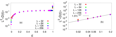
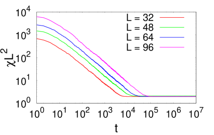
Eq. (2) shows that one can approximately regard the variation of $\rho(t)$ as a power law decay. The dominating term at large times being proportional to $\ln(t)/t$, the approximate value of the exponent would be somewhat less than 1. Fig. 1 shows that it is possible to collapse the data for different system sizes with appreciable accuracy using suitable scaling factors. Assuming that $\rho(t)$ approximately decays as $t^{-\mu}$, the data collapse occurs with the following scaling form:

$$\rho(t,L)=L^{-y}f(t/L^{z}).$$ (3)

To regain the form $\rho(t)\sim t^{-\mu}$ for large $L$, the scaling function $f(x)$ must behave as $x^{-\mu}$ such that

$$y=z\mu.$$ (4)

The best collapse was found with $y=2$ and $z=2.25$ for $\varepsilon=0$, giving $\mu\approx 0.9$ (Fig. 1(a)).

Figure 1: Data collapses of $\rho(t,L)$ for (a) $\varepsilon=0$ and (b) $\varepsilon=1$. Insets show the unscaled data.

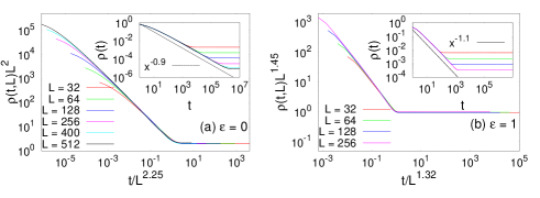
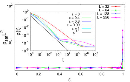
As $\varepsilon$ is made non-zero, three different regions emerge in the behavior of $\rho(t)$. Initially there is a fast decay followed by a slower decay and at later stages, a saturation region appears (inset of Fig. 2). The intermediate region of slower decay is prominently observed for $0<\varepsilon<1$, but vanishes at $\varepsilon=1$ and $0$. The form of $\rho(t)$ for $\varepsilon=0$ given by Eq. (2) is not seen to be followed for any nonzero value of $\varepsilon$. Nevertheless, for $\varepsilon=1$, an analysis similar to that made for $\varepsilon=0$ can be attempted to obtain an effective exponent. We find a nice collapse for the data for different system sizes using the values $y=1.45$ and $z=1.32$ (Fig. 1(b)). Thus the effective decay exponent $\mu$ for $\rho(t)$ is $\approx 1.1$ which is different from that of $\varepsilon=0$. In fact the initial faster decay region for all $\varepsilon>0$ appears to have an approximate power law behavior with the value of the exponent $\mu$ varying between 1.3 and 1.1 (shown in inset of Fig. 2). It is to be noted here that for $\varepsilon=0$ the estimate of $z$ can be made more accurate by using the exact variation of $\rho(t)$ (see section IV), the present estimate is only to make a fair comparison with the $\varepsilon=1$ case.

We next study $\rho_{sat}$, the saturation value of the density of the particles as a function of $\varepsilon$. In section I it was mentioned that one expects three possibilities: zero, only one or two surviving particles at steady state even for the unbiased case. This will make $\rho_{sat}$, the saturation value, vanishingly small as the system size is increased. Indeed, for $\varepsilon<1$, $\rho_{sat}$ is found to be $\ll 1$, vanishing as $1/L^{2}$. However for $\varepsilon=1$, $\rho_{sat}$ is one order of magnitude higher than those for $\varepsilon<1$ (inset of Fig. 2). This indicates that a much larger number of particles remain in the system at the steady state for $\varepsilon=1$. Indeed, the total number of remaining particles $\rho_{sat}L^{2}$ shows an abrupt increase at $\varepsilon=1$ as shown in Fig. 2. In fact for $\varepsilon=1$, $\rho_{sat}L^{2}$ increases with system size while for $\varepsilon\neq 1$, $\rho_{sat}L^{2}$ is fairly a constant.

Figure 2: $\rho_{sat}L^{2}$ shown against $\varepsilon$. Inset shows the variation of $\rho(t)$ as a function of time $t$ for a system size of $256\times 256$ for several values of $\varepsilon$.

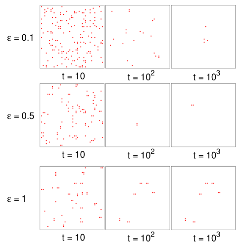
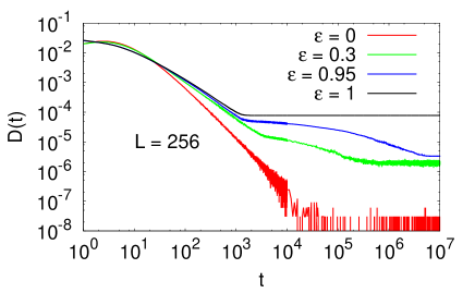
At $\varepsilon=1$, it can be easily understood that at long times when few particles are left, as two particles always approach each other, a situation will emerge when they may appear on neighbouring sites with no other neighboring sites occupied. Fig. 3 shows the snapshots at different times for different values of $\varepsilon$ and at large times for $\varepsilon=1$, one notes that such pairs will survive indefinitely. This is because the subsequent dynamics will simply be a swapping of the positions of the two neighbouring particles. These two particles form what we call a dimer. A dimer is defined to be a pair of particles occupying neighbouring sites and both the particles do not have any other neighbour. As these particles will never get annihilated at $\varepsilon=1$, it is expected that there will be a larger number of surviving particles. To probe this in more detail, we calculate $D(t)$, the density of dimers in the system for all $\varepsilon$ values. $D(t)$ is the number of dimers divided by $L^{2}$. The data shown in Fig. 4 clearly show a larger value of $D(t)$ for $\varepsilon=1$ in the steady state compared to other $\varepsilon$ values as expected. However, surprisingly, a non-zero saturation value is found for other values of $\varepsilon>0$ also. At $\varepsilon=0$, the value of $D(t)$ at large times becomes negligibly small ($\mathcal{O}(10^{-8})$). This is expected as even though two particles can remain in the steady state the probability of forming dimers for $\varepsilon=0$ is negligible, as the particles have equal probability of moving to other neighboring sites.

Figure 3: Snapshots of a $40\times 40$ system for $\varepsilon=0.1,0.5$ and $1$ at $t=10,10^{2}$ and $10^{3}$. Cases for $\varepsilon=0.5$ and $1$ shows the formation of dimers. For $\varepsilon=1$ the dimers are seen to persist.

Figure 4: Variation of $D(t)$ as a function of time $t$ for several $\varepsilon$ values for system size of $256\times 256$.

Figure 5: (a) Variation of $\langle D(t)\rangle$ in the steady state multiplied by $L^{2}$ with $\varepsilon$ for several system sizes. (b) Power law behavior of this quantity close to $\varepsilon=0$.

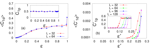
Studying the saturation values of the actual number of dimers, $\langle D(t)\rangle L^{2}$ ($\langle...\rangle$ indicates a thermal average in the steady state) against $\varepsilon$ (Fig. 5(a)), we note that it has a nonzero finite value increasing with $\varepsilon$ (independent of $L$ for $\varepsilon<1$) and a jump at $\varepsilon=1$ (increasing with $L$). Close to $\varepsilon=0$, $L^{2}\langle D(t)\rangle$ shows a power law behavior with $\varepsilon$ in the form $\sim\varepsilon^{\eta}$ with $\eta=1.67\pm 0.04$ (Fig. 5(b)).

For nonzero $\varepsilon$ therefore, the steady state can have several possibilities: (i) zero, one, or two isolated particles (ii) dimers (iii) coexistence of dimers and isolated particles. For $\varepsilon=1$, the last case will not arise. Let us, for the sake of argument, assume that it is possible to have a state comprising of a dimer and an isolated particle. The dimer will remain static in its position, while the isolated particle will travel to form a “trimer”, which is unstable and will decay immediately into an isolated particle. When $N_{p}(t)$, the number of particles present at time $t$ is even, the maximum number of dimers that can be formed is $N_{p}(t)/2$. We hence define,

$$d_{r}(t)=\frac{2D(t)L^{2}}{N_{p}(t)}$$ (5)

as the probability that a dimer is formed out of the remaining particles. We note that $d_{r}(t)\rightarrow 1$ in a finite time for $\varepsilon=1$. Therefore, if an even number of particles survive for $\varepsilon=1$, all of them will form dimers. Of course, states with either zero or a single surviving particle are also possible for $\varepsilon=1$. These features have all been checked in the simulation.

To get an idea which kind of steady states are more prevalent, we calculate $C_{1p}$, the fraction of cases for which the system is left with a single particle. $C_{1p}$ is found to be nearly 0.5 for all $\varepsilon$ (inset of Fig. 6(a)). We also calculate $\langle C_{1d}\rangle$, the probability of getting at least one dimer which turns out to be an increasing function of $\varepsilon$, showing a jump at $\varepsilon=1$ (Fig. 6(a)). Although the probability is less than 0.5, still it is quite appreciable ($\mathcal{O}(10^{-1}$)).

Figure 6: Variation of (a) $\langle C_{1d}\rangle$ and $C_{1p}$ with $\varepsilon$ and that of (b) $\langle C^{\prime}_{1d}\rangle$ and $C^{\prime}_{1p}$ with $\varepsilon^{\prime}$.

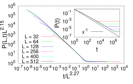
To calculate the persistent probability $P(t)$, the initially occupied sites are regarded as unvisited. For $\varepsilon=0$ the persistence probability $P(t)$ was calculated for a maximum size $L=512$ and it shows a power law decay: $P(t)\sim t^{-\theta}$ with $\theta\simeq 1$ (inset of Fig. 7). This value of the persistence exponent obtained for parallel dynamics, is also, therefore, approximately twice the value for asynchronous dynamics, as was found in the one dimensional spin models ray-mapping ; potts . Finite size scaling analysis was performed using the scaling ansatz manoj

$$P(t,L)L^{\alpha}=g(t/L^{z_{p}}),$$ (6)

and a data collapse was obtained with $\alpha=2.15$ and $z_{p}=2.27$ such that $\theta=\alpha/z_{p}\approx 0.95$. The results are shown in Fig. 7. As $\varepsilon$ is increased, $P(t)$ deviates from the power law behavior and saturates to higher values. Since annihilations are enhanced for nonzero $\varepsilon$, a higher saturation value is obtained as $\varepsilon$ is increased.

Figure 7: Data collapse of $P(t)$ for $\varepsilon=0$ using Eq. (6). Inset shows the unscaled data.

IV Results for case II

In the simulation for Case II dynamics, a particle is allowed to move one step towards its nearest particle with probability $\varepsilon^{\prime}$ and with probability $1-\varepsilon^{\prime}$ it goes to one of the three remaining nearest neighboring positions. The annihilations take place in the usual manner. The region $0.25<\varepsilon^{\prime}\leq 1$ of Case II corresponds to $0<\varepsilon\leq 1$ of Case I, where the particles have the tendency to approach their nearest particle on the lattice, i.e., the bias is positive.

We first check the validity of Eq. (1) using the Case II dynamics; specifically it is verified where the diffusive point lies. Here it should be mentioned that when the particle does not choose to move to a site that brings it closer to its nearest particle, it moves to one of the remaining three neighbouring sites. This implies that the fact that one of these movements may also take it closer to its nearest particle is ignored. Hence one can expect a validity of Eq. (1) only in the thermodynamic limit, as argued in section II.

As the annihilations become less probable for negative bias, the system takes a very long time to attain the steady state and in the simulations, for larger system sizes, the system may not attain the steady state within the maximum number of Monte Carlo steps. Nevertheless, some essential information could be extrapolated from the results obtained in the nonequilibrium region.

At $\varepsilon^{\prime}=0$, the particles are completely repulsive and even at very long times, one may expect a nonzero density of particles for small $\varepsilon^{\prime}$. At the diffusive limit on the other hand, the number of remaining particles being either zero, 1 or 2, $\rho(t\to\infty)\to 0$. It is also highly unlikely that dimers will be formed with the negative bias and one expects the number of configurations with dimers to be equal to zero till the diffusive point. As in Case I, here too we estimate $C_{1p}^{\prime}$ and $\langle C_{1d}^{\prime}\rangle$, the probabilities of getting a single surviving particle and at least one dimer respectively. The results are shown in Fig. 6(b). $\langle C_{1d}^{\prime}\rangle$ clearly shows an abrupt rise close to $\varepsilon^{\prime}=0.25$ as the system size increases, which supports the fact that the diffusive point lies at $\varepsilon^{\prime}=0.25$. $C_{1p}^{\prime}$ also shows an abrupt rise, however, here the finite size effects are stronger and the abrupt rise takes place at a value of $\varepsilon^{\prime}$ which slowly approaches 0.25. Hence the diffusive point, denoted by ${\varepsilon_{c}}^{\prime}=0.25$ in the thermodynamic limit, depends on the system size. A detailed study of $\rho(t)$ given in the following indicates that the remaining fraction of particles at very large times varies as $({\varepsilon_{c}}^{\prime}-\varepsilon^{\prime})^{\beta}$, where ${\varepsilon_{c}}^{\prime}=0.25$ and $\beta\approx 2$. The sharp decrease of $\rho$ for $\varepsilon^{\prime}$ close to ${\varepsilon_{c}}^{\prime}$ implies there could be a finite number of configurations having only one remaining particle even for $\varepsilon^{\prime}<0.25$ and this explains why $C_{1p}^{\prime}$ shows the abrupt increase at a lower value of $\varepsilon^{\prime}$ compared to 0.25, even for the maximum size considered.

Figure 8: (a) Variation $\rho(t)$ as a function of time $t$ for $L=128$ for several values of $\varepsilon^{\prime}$. (b) Data collapse of $\rho(t)$ for $L=128$ for several values of $\varepsilon^{\prime}$ using the scaling form Eq. (12).

Figure 9: Variation of $\rho_{\infty}$ as a function of ${\varepsilon_{c}}^{\prime}-\varepsilon^{\prime}$ for $L=128$. The data was fitted according to the function 0.124$({\varepsilon_{c}}^{\prime}-\varepsilon^{\prime})^{\beta}$, with $\beta=1.923\pm 0.05$. Inset shows the fitting of a $\rho(t)$ curve for $L=128$, $\varepsilon^{\prime}=0.2$ according to the function $\rho_{\infty}+k_{1}t^{-\lambda}$, with $\rho_{\infty}=0.004\pm 10^{-6}$, $k_{1}=0.0819\pm 10^{-4}$ and $\lambda=0.34\pm 10^{-4}$.

Figure 10: (a) Variation of $\rho$ at $t_{max}=10^{7}$ as a function of $\varepsilon^{\prime}$. $\rho(t_{max})$ reaches a plateau at ${\varepsilon_{c}}^{\prime}(L)$. (b) Data collapse of $\rho(t_{max})$ for several system sizes using the scaling relation given by Eq. (9). The scaled form varies as $({\varepsilon_{c}}^{\prime}-\varepsilon^{\prime})^{2}$ for $\varepsilon^{\prime}<{\varepsilon_{c}}^{\prime}$ (shown by the solid line).

Figure 11: (a) Variation of $({\varepsilon_{c}}^{\prime})_{eff}$ with $1/L$. The data is fitted according to the curve $0.25-2.125x^{1/1.131}$. (b) Data collapse of $\rho(t)$ for several system sizes at $\varepsilon^{\prime}=0.25$ using the scaling form Eq. (12).

Next, we analyse the behaviour of $\rho(t)$ in detail. For the largest size simulated, $L=128$, the data are shown in Fig. 8(a) and fitted to the form

$$\rho(t)=\rho_{\infty}+k_{1}t^{-\lambda}$$ (7)

(inset of Fig. 9). We find a good consistency in the fittings for $t>10^{4}$. It is found that

$$\rho_{\infty}\sim({\varepsilon_{c}}^{\prime}-\varepsilon^{\prime})^{\beta},$$ (8)

with $\beta=1.92\pm 0.05$ (Fig. 9), while $\lambda$ increases with $\varepsilon^{\prime}$, since convergence is reached faster for larger value of $\varepsilon^{\prime}$.

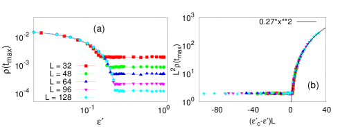
The above result is also consistent with a finite size analysis when $\rho(t_{max})$ is studied for different values of $L$ and one can argue that $\beta\approx 2$. Here, $t_{max}$ is the maximum number of Monte Carlo steps up to which the simulations were performed. The unscaled data is shown in Fig. 10(a). We find the following scaling behaviour of $\rho(t_{max})$:

$$\rho(t_{max})L^{s}=f_{1}\Big{(}({\varepsilon_{c}}^{\prime}-\varepsilon^{\prime})L^{\alpha^{\prime}}\Big{)},$$ (9)

with $s=2$ and $\alpha^{\prime}=1$ (Fig. 10(b)). The scaling function behaves as

$$f_{1}(x)=\begin{cases}{\rm const}&\text{for $\varepsilon^{\prime}>{\varepsilon_{c}}^{\prime}$}\\ x^{2}&\text{for $\varepsilon^{\prime}<{\varepsilon_{c}}^{\prime}$}.\end{cases}$$ (10)

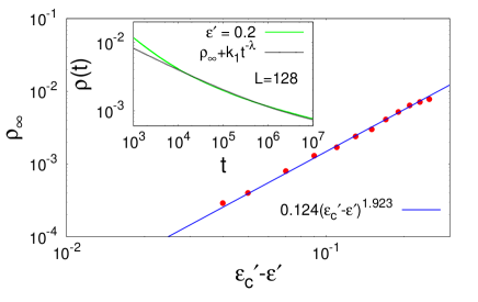
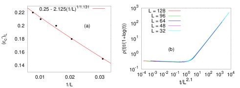
This implies that $\rho(t_{max})$ varies as $L^{-2}$ for $\varepsilon^{\prime}>{\varepsilon_{c}}^{\prime}$ and as $({\varepsilon_{c}}^{\prime}-\varepsilon^{\prime})^{2}$ for $\varepsilon^{\prime}<{\varepsilon_{c}}^{\prime}$. The scaling variable being $({\varepsilon_{c}}^{\prime}-\varepsilon^{\prime})L$, we conjecture that there is a diverging length scale $L\sim({\varepsilon_{c}}^{\prime}-\varepsilon^{\prime})^{-1}$. In support of this, we study the variation of the effective critical value ${\varepsilon_{c}}^{\prime}(L)$, determined by the value of $\varepsilon^{\prime}$ at which $\rho$ attains a constant value as a function of $\varepsilon^{\prime}$ (shown in Fig. 10(a)) for the system size $L$. $\varepsilon_{c}^{\prime}(L)$ is found to obey the familiar scaling form for a continuous phase transition

$$\varepsilon_{c}^{\prime}(L)=\varepsilon_{c}^{\prime}-{\mathcal{O}}(\frac{1}{L^{1/\nu}}),$$ (11)

shown in Fig. 11(a). Here, $\nu=1.13\pm 0.06$, which is close to 1, consistent with the finite size scaling analysis of $\rho(t_{max},L)$. We conclude that $\rho$ behaves like an order parameter that vanishes at the critical point $\varepsilon_{c}^{\prime}$ with the critical exponent values $\beta\approx 2$ and $\nu\approx 1$.

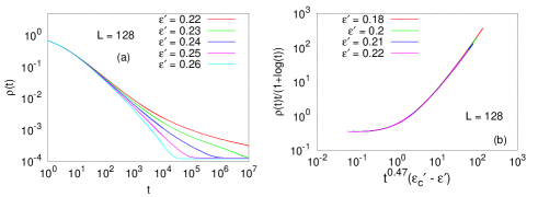
The presence of a diverging time scale can also be detected when we note that a data collapse for $\rho(t)$ for $L=128$ is obtained in the following form

$$\rho(t)\Big{(}\frac{1+\log(t)}{t}\Big{)}^{-1}=f_{2}\big{(}t^{a_{1}}({\varepsilon_{c}}^{\prime}-\varepsilon^{\prime})\big{)}$$ (12)

with $a_{1}=0.47\pm 0.04$ (shown in Fig. 8(b)). This shows that the diverging time scales as $({\varepsilon_{c}}^{\prime}-\varepsilon^{\prime})^{1/a_{1}}$. Hence, the dynamic exponent is $1/a_{1}\approx 2.1$. Also, we have been able to conduct a finite size scaling analysis of $\rho(t)$ exactly at criticality for different system sizes using the form

$$\rho(t)\Big{(}\frac{1+\log(t)}{t}\Big{)}^{-1}=f_{3}(t/L^{z}).$$ (13)

Once again we find a good collapse with $z\approx 2.1$. This result is shown in Fig. 11(b). It is to be noted that in Eqs. (12) and (13) we have used the exact form of $\rho(t)$ for $L\to\infty$.

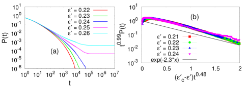
Finally, the persistence probability $P(t)$ is studied; for small $\varepsilon^{\prime}$ it shows a fast decay and goes to zero. Above a certain value of $\varepsilon^{\prime}$, $P(t)$ saturates to a non-zero value. From Fig. 12(a) we can see that $P(t)$ changes in nature at $\varepsilon^{\prime}\approx 0.25$. This is consistent with the fact that in the small $\varepsilon^{\prime}$ region the particles have a tendency to move away from its nearest walker, thereby reducing the probability of annihilation and allowing the particles to roam around more. For $\varepsilon^{\prime}>0.25$, the particles annihilate at a faster rate, such that a large number of sites can remain unvisited, as already discussed in section III.

For the system size $L=128$, the data for $P(t)$ are collapsed according to the following form,

$$P(t)=t^{-0.99}f^{\prime}\Big{(}t^{0.48}({\varepsilon_{c}}^{\prime}-\varepsilon^{\prime})\Big{)}.$$ (14)

This has been shown in Fig. 12(b). $f^{\prime}$ shows an exponential decay for large values of the argument such that for large $t$, $P(t)$ varies as $t^{-0.99}\exp\big{(}t^{0.48}({\varepsilon_{c}}^{\prime}-\varepsilon^{\prime})\big{)}$. This form is consistent with the power law behaviour at the critical point as obtained in the previous section.

Figure 12: (a) Variation of persistence probability $P(t)$ as a function of time $t$ for a $128\times 128$ system for several values of $\varepsilon^{\prime}$. (b) Data collapse of $P(t)$ using the scaling form given by Eq. (14). The collapsed form shows a variation of the form $\exp({-t/\tau})$.

Figure 13: Scaling collapse of the steady state values of susceptibility $\chi$ for several system sizes at the critical point ${\varepsilon_{c}}^{\prime}=0.25$.

V Discussions and concluding remarks

In this paper we have studied the time evolution of a single species reaction diffusion system where the particles perform nearest neighbour hops on a lattice with a bias to move towards the nearest particle. The bias can be made both positive and negative (Case II) parametrically. The particles are annihilated if they are found on the same site after the completion of one Monte Carlo step. A diffusive motion occurs for individual particles when the parameter $\varepsilon^{\prime}=0.25$, above (below) this value, the particles have attractive (repulsive) motion.

The dynamical evolution of the density of particles $\rho(t)$ is studied and as expected, for $\varepsilon^{\prime}=0.25$, $\rho(t)$ vanishes in the thermodynamic limit as the number of surviving particles can be zero, one or two. The region where $\rho(t\to\infty)$ remains finite is $\varepsilon^{\prime}<\varepsilon^{\prime}_{c}=0.25$; the extrapolated data for the maximum size simulated as well as a finite size scaling analysis indicate $\rho(t\to\infty)$ varies as $({\varepsilon_{c}}^{\prime}-\varepsilon^{\prime})^{2}$.

Although $\rho(t)$ is still vanishingly small for $\varepsilon^{\prime}>0.25$, the decay of $\rho(t)$ takes place in a manner distinctly different from that of $\varepsilon^{\prime}=0.25$. Moreover, a discontinuity occurs at $\varepsilon^{\prime}=1$, the fully positively biased point where the particles invariably move towards the nearest particles. On probing deeper, we find a dimerisation taking place for any $\varepsilon^{\prime}>0.25$, the number of dimers as well as the probability shows a jump at $\varepsilon^{\prime}=1$. The variation of the number of dimers (although its density is vanishingly small) shows a continuous increase from zero at the diffusive point; $\langle D(t)\rangle L^{2}\propto(\varepsilon^{\prime}-0.25)^{\eta}$, where $\eta$ is very close to 5/3.

The diffusive behaviour therefore occurs at a single point of the parameter space. This is reminiscent of the generalised voter model in two dimensions where the voter model occurs at a single point of the two dimensional parameter space gen-voter . The diffusive point separates two regions marked by completely different features: to its left one has a nonzero value of $\rho(t\to\infty)$ and to the right, a nonzero number of dimers, both vanishing in a power law manner with different exponents. The persistence probability also shows different behaviour for $\varepsilon^{\prime}<0.25$ and $\varepsilon^{\prime}>0.25$. For $\varepsilon^{\prime}<0.25$, it goes to zero in a stretched exponential manner while in the other region it attains a nonzero value at large times for $\varepsilon^{\prime}>0.25$. Exactly at the diffusive point it shows a power law decay.

We have concluded that a continuous phase transition takes place at $\varepsilon^{\prime}=0.25$. $\rho(t\to\infty)$ behaves as an order parameter that vanishes continuously as $(\varepsilon_{c}^{\prime}-\varepsilon^{\prime})^{\beta}$. The phase transition is similar to that studied recently in daga . The presence of a diverging length scale as well as a diverging timescale have been detected as ${\varepsilon_{c}}^{\prime}\to 0.25$ with exponents $\nu\approx 1$ and $z$ lying between 2.1 and 2.2, obtained using several different finite size scaling analyses.

One interesting point to be noted is that as $\nu\approx 1$, $\alpha$, the critical exponent for the specific heat must be zero according to the scaling relation $\nu d=2-\alpha$ as $d=2$. In order to satisfy the scaling relation $\alpha+2\beta+\gamma$ =2, where $\gamma$ is the critical exponent for susceptibility, $\gamma$ has to be negative. Indeed, we find that the steady state value of the susceptibility defined as $\chi=\big{(}\langle\rho^{2}\rangle-\langle\rho\rangle^{2}\big{)}L^{2}$ gyorgy , varies as $L^{-2}$ such that $\gamma=-2\nu\approx 2$ (shown in Fig. 13). The susceptibility not showing a divergence at the critical point is a counter-intuitive result, however, such a behaviour is not unprecedented and was also observed for the dynamical models studied in lalla ; psen . The anomalous behaviour of the susceptibility could be due to the fact that the system here involves long range interactions which can affect the values of the exponents non-trivially.

In general, asynchronous and parallel dynamics are expected to affect the dynamics differently; however, at least for the diffusive limit $\varepsilon^{\prime}=0.25$, the form of $\rho(t)$ is identical for both types of dynamics. Interestingly, the persistence exponent for the parallel dynamics is found to be twice of that for the asynchronous, a result similar to the case for one dimensional spin models but by no means obvious. The formation of the dimer patterns is an artifact of the parallel updating scheme.

Acknowledgement: This work was inspired by a comment made by Subir K. Das. Useful discussions with Purusattam Ray and Bikas Chakrabarti are acknowledged. P. Mullick thanks DST-INSPIRE (Sanction No. 2015/IF0673) for their financial support. P. Sen acknowledges SERB (Scheme no EMR/2016/005429, Government of India) for financial grant.

References

- (1) See e.g. T. M. Ligget, Interacting Particle Systems, Springer-Verlag, New York, (1985); V. Privman, ed, Nonequlibrium Statistical Mechanics in One Dimension, Cambridge University Press, Cambridge (1997); P. L. Krapivsky, S. Redner and E. Ben-Naim, A Kinetic View of Statistical Physics, Cambridge Universiy Press, Cambridge (2009) and the references therein.
- (2) Z. Racz, Phys. Rev. Lett. 55, 1707 (1985).
- (3) J. L. Spouge, Phys. Rev. Lett. 60, (1988) 871.
- (4) J. G. Amar and F. Family, Phys. Rev. A 41, 3258 (1990).
- (5) D. ben-Avraham, M. A. Burschka, and C. R. Doering, J. Stat. Phys. 60, 695 (1990).
- (6) F. C. Alcaraz, M. Droz, M. Henkel and V. Rittenberg, Ann. Phys. 230, 250 (1994).
- (7) K. Krebs, M. P. Pfannmuller, B. Wehefritz and H. Hinrinchsen, J. Stat. Phys. 78, 1429 (1995).
- (8) J. E. Santos, G. M. Schutz and R. B. Stinchcombe, J. Chem. Phys. 105, 2399 (1996).
- (9) G. M. Schutz, Z. Phys. B 104, 583 (1997).
- (10) K. Sasaki and T. Nakagawa, J. Phys. Soc. Japan 69, 1341 (2000).
- (11) D. ben-Avraham and E. Brunet, J. Phys. A 38, 3247 (2005).
- (12) M. J. de Oliveira, Brazilian Journal of Physics 30 128 (2000).
- (13) K. Kang and S. Redner, Phys. Rev. A 30, 2833 (1984); 32, 435 (1985).
- (14) G. Zumofen, A. Blumen and J. Klafter, J. Chem. Phys. 82, 3198 (1985).
- (15) L. Peliti, J. Phys. A 19, L365 (1986).
- (16) M. Droz and L. Sasvari, Phys. Rev. E 48, R2343 (1993).
- (17) B. P. Lee, J. Phys. A 27, 2633 (1994).
- (18) J. Cardy, J. Phys. A.: Math. Gen. 28, L19 (1995).
- (19) J. L. Cardy and U. C. Tauber, J. Stat. Phys. 90, 1 (1998).
- (20) G. Szabò and M. A. Santos, Phys. Rev. E 59, R2509 (1999).
- (21) Two particles will survive in the parallel dynamics for a special case only. One can regard the two dimensional lattice as a checkerboard with the particles occupying either black or white squares. If the last two survivors are on different coloured squares, in a parallel dynamics they will never meet and annihilate. However for asynchronous dynamics, they will be annihilated ultimately, even if it takes a long time.
- (22) A. J. Bray, S. N. Majumdar, G. Schehr, Adv. Phys. 62, 225 (2013).
- (23) S. Biswas, P. Sen and P. Ray, J. Phys. Conf. Series 297, 012003 (2011).
- (24) P. Sen and P. Ray, Phys. Rev. E 92, 012109 (2015)
- (25) S. Biswas and P. Sen, Phys. Rev. E 80, 027101 (2009).
- (26) P. Turchin, Quantitative analysis of movement: measuring and modelling population redistribution in animals and plants, Sunderland, MA: Sinauer Associates, Inc. Publishers (1998).
- (27) H. J. Blok and B. Bergersen, Phys. Rev. E 59, 3876 (1999).
- (28) B. Derrida, V. Hakim and V. Pasquier, Phys. Rev. Lett. 75, 751 (1995).
- (29) G. I. Menon, P. Ray and P. Shukla, Phys. Rev. E 64, 046102 (2001).
- (30) G. I. Menon and P. Ray, J. Phys. A: Math. Gen. 34, L735 (2001).
- (31) In gyorgy , Eq. (2) was written in terms of instead of natural . Making the necessary conversion, the value of is found to be very close.
- (32) G. Manoj and P. Ray, Phys. Rev. E 62, 7755 (2000).
- (33) M. J. de Oliveira, J. F. F. Mendes and M. A. Santos, J. Phys. A: Math. Gen. 26, 2317 (1993).
- (34) B. Daga and P. Ray, Phys. Rev. E 99, 032104 (2019).
- (35) M. Lallouache, A. S. Chakrabarti, A. Chakraborti and B. K. Chakrabarti, Phys. Rev. E 82, 056112 (2010).
- (36) P. Sen, Phys. Rev. E 83, 016108 (2011).