The distribution of heavy-elements in giant protoplanetary atmospheres: the importance of planetesimal-envelope interactions

Abstract

In the standard model for giant planet formation, the planetary growth begins with accretion of solids followed by a buildup of a gaseous atmosphere as more solids are accreted, and finally, by rapid accretion of gas. The interaction of the solids with the gaseous envelope determines the subsequent planetary growth and the final internal structure. In this work we simulate the interaction of planetesimals with a growing giant planet (proto-Jupiter) and investigate how different treatments of the planetesimal-envelope interaction affect the heavy-element distribution, and the inferred core mass. We consider various planetesimal sizes and compositions as well as different ablation and radiation efficiencies, and fragmentation models. We find that in most cases the core reaches a maximum mass of $\sim$ 2 M_⊕. We show that the value of the core’s mass mainly depends on the assumed size and composition of the solids, while the heavy-element distribution is also affected by the fate of the accreted planetesimals (ablation/fragmentation). Fragmentation, which is found to be important for planetesimals $>$ 1 km, typically leads to enrichment of the inner part of the envelope while ablation results in enrichment of the outer atmosphere. Finally, we present a semi-analytical prescription for deriving the heavy-element distribution in giant protoplanets.

1 Introduction

The ongoing characterization and discoveries of giant exoplanets and the accurate measurements of the giant planets in the Solar System provide a unique opportunity to understand these astronomical objects. As more information is available, theoretical models are challenged to explain the observed properties. This is not always an easy task, in particular when we aim to connect giant planetary interiors with giant planet formation (e.g., Helled & Lunine 2014).

In the standard model for giant planet formation, core accretion, the planetary growth begins with the formation of a core (Alibert et al. 2005, Pollack et al. 1996, Helled et al. 2014 and references therein). Once the core reaches about Mars’ mass, its gravity is strong enough to bind hydrogen and helium (hereafter H-He) gas from the protoplanetary disk. Then, the protoplanet keeps growing by accreting both solids (heavy elements) and H-He until crossover mass is reached and rapid gas accretion takes place. In the early core accretion simulations for the sake of numerical simplicity, it was assumed that all the heavy elements reach the core while the envelope is composed of H-He (Pollack et al., 1996). During the initial stages of planetary formation, the proto-planet is capable of binding only a very tenuous envelope, so that infalling planetesimals reach the core directly (e.g., Pollack et al. 1996). Once the core mass reaches a small value of $\sim$ 1-2 M_⊕ (Pollack et al., 1986; Brouwers et al., 2017; Iaroslavitz & Podolak, 2007; Venturini et al., 2016; Lozovsky et al., 2017) and is surrounded by gas, solids (planetesimals/pebbles) composed of heavy-elements are expected to dissolve in the envelope instead of reaching the core.

While it is known that the heavy elements can remain in the envelope, their actual distribution is not well constrained. Nevertheless, determining the fate of the accreted heavy elements and their distribution within the envelope is important for several reasons. First, a non-homogenous internal structure has a significant impact on the thermal evolution and final structure of the planets (Lozovsky et al. 2017,Vazan et al. 2018). Second, the presence of heavy elements material in the envelope can dramatically affect the consequent growth of the planet (Hori & Ikoma 2011,Venturini et al. 2016). Finally, the deposition of heavy elements can change the local conditions at the envelope such as the opacity and heat transport mechanism. Despite its importance, envelope enrichment is often neglected, or being treated in a simple manner. This is mainly due to the difficulty in following the planetesimal-envelope interaction in detail and at the same time model the subsequent planetary growth while accounting for the change in the equation of state and opacity of the envelope due to heavy-element deposition. These two aspects involve different physical processes, and therefore studies typically concentrate on the interaction between heavy elements and the planetary envelope (e.g., Venturini et al. 2016,Lozovsky et al. 2017, Brouwers et al. 2017) or on the effect of the heavy-elements on planetary growth and long-term evolution (e.g., Vazan et al. 2018).

Previous research on planetesimal ablation in giant protoplanets has been mostly focused on the inferred core mass. While using different approaches, several studies predicted a small core mass between 0.2 - 5 M_⊕ for giant protoplanets. Already in Pollack et al. (1986) it was shown that the maximum core mass when considering accretion of $100$ km-sized planetesimals is between $1$ and $3$ M_⊕. Brouwers et al. (2017) investigated the growth of the core with accretion of pebbles/planetesimal at early stages. It was found that pebble accretion leads to a core with a maximum mass between 0.1 - 0.6 M_⊕ depending on the pebbles’ composition. For the case of 1 km-sized rocky planetesimals a maximum core mass between $0.2-1.2$ M_⊕ was derived. It was shown that the predicted core mass depends on the assumed material strength of rock and its effect on the planetesimal’s ablation/fragmentation. Alibert (2017) performed a similar study, investigating the envelope’s mass required to disrupt $10$ cm-sized pebbles. It was found that an envelope with a mass of $0.001$ M_⊕ is sufficient to destroy the pebbles. The mass of the core was found to be between $0.5$ and $3$ M_⊕. Lozovsky et al. (2017) investigated the distribution of heavy elements in proto-Jupiter accounting for different solid surface densities and planetesimal sizes. A maximum core mass of 2-3 M_⊕ was found with the rest of the heavy elements having a gradual distribution throughout the planet. It was also shown that further settling of the heavy elements is negligible. All of the studies mentioned above support the concept of a small core for giant planets. However, it should be noticed that similar studies by Mordasini et al. (2006) and Baraffe et al. (2006) derive core masses of $\sim$ $5$-$6$ M_⊕. Possible reasons for the higher inferred core masses could be different treatments of fragmentation, and different assumed material strengths and $C_{h}$ values (see discussions below).

A fundamental aspect in predicting the heavy-element distribution in proto-Jupiter (and giant protoplanets in general) is linked to the interaction of the solids (which can be pebbles or planetesimals) with the planetary envelope. The fate of the heavy elements is uncertain and depends on the physical properties of the accreted planetesimals and of the gaseous envelope. In addition, the distribution could depend on the treatment of planetesimal fragmentation and ablation. In this study, we explore the interaction of the heavy elements with the gaseous envelope accounting for the ablation and fragmentation of planetesimals and determine the heavy-element distribution within the planet. We also investigate the dependence of the heavy-element distribution and inferred core mass on the planetesimals’ properties and the treatment of the planetesimal-envelope interaction. Finally, we present a simple semi-analytical approach for deriving the heavy-element distribution.

2 Methods

The interaction of a planetesimal with the planetary envelope is simulated following the approach of Podolak et al. (1988) where at each step of the two dimensional trajectory we compute the planetesimal’s motion in response to gas drag and gravitational forces (assuming a 2-body interaction). The effects of planetesimal heating and ablation as the planetesimal passes through the envelope are also included. We also consider planetesimal fragmentation which is set to occur when the pressure gradient of the surrounding gas across the planetesimal exceeds the material strength and the planetesimal is small enough that self-gravity cannot counteract the disruptive effect of the pressure gradient, and is given by (Pollack et al., 1986):

$$P={\frac{1}{2}}\rho_{gas}v^{2}\geq S,$$ (1)

$$r_{p}<r_{dyn}=\sqrt{\frac{5v^{2}\rho_{gas}}{8\pi G\rho_{p}^{2}}},$$ (2)

where $P$ is the pressure, $v$ is the planetesimal’s velocity, $\rho_{gas}$ is the envelope’s density, $S$ is the compressive material’s strength depending on the planetesimal’s composition, $\rho_{p}$ and $r_{p}$ are the planetesimal’s density and radius, respectively. We have implemented several improvements to the new computation. First, we include an adaptive step size control to the 4th order Runge-Kutta method that is used to solve the equation of motion. Instead of evaluating the equation of motion once per time step, we do it three times; once as a full step, and then, independently, as two half steps until convergence is found. Second, we use an improved model for the planetesimal’s fragmentation. In Podolak et al. (1988) when a planetesimal fragments it was assumed that the entire planetesimal mass is deposited in that layer, while we continue to follow the planetesimal’s fragments considering different fragmentation models (see section 4.1). Further details on the atmosphere-planetesimal interaction are presented in the Appendix.

The equations describing the motion and mass loss of a planetesimal in the planetary envelope are:

$$m_{pl}\frac{d\vec{v}}{dt}=-\Gamma A\rho_{gas}\left|v\right|\vec{v}-G\frac{M_{p}(r)m_{pl}}{r^{3}}\vec{r},$$ (3)

$$\frac{dm_{pl}}{dt}=-\frac{A}{Q}\bigg{(}\frac{1}{2}C_{h}\rho_{gas}\left|v\right|^{3}+\epsilon\sigma T_{a}^{4}\bigg{)}.$$ (4)

The first is the equation of motion in 2D, where $m_{pl}$ is the planetesimal’s mass, $\Gamma$ is the drag coefficient (calculated as in Podolak et al. (1988)), $A$ is the planetesimal’s surface, $r$ is the distance from the protoplanet’s center and $M_{p}(r)$ is the planet’s mass inside $r$. The second equation describes the planetesimal’s ablation where $T_{a}$ is the atmospheric background temperature and $\sigma$ is the Stefan-Boltzmann constant. There are two sources for ablation: the radiation from the surrounding atmosphere and gas drag. For simplicity, the atmosphere is assumed to behave as a gray body, $\epsilon$ is the emissivity which is a product of the emissivity of the atmospheric gas and the absorption’s coefficient of the impactor. The value of $\epsilon$ is not well-determined and depends on the local density, pressure, temperature, and composition of the atmosphere. Therefore, we assume different $\epsilon$ values, and investigate their impact on the results. $Q$ is the latent heat caused upon vaporization, and $C_{h}$ is the heat transfer coefficient. $C_{h}$ is the fraction of the relative kinetic energy transferred to the planetesimal and its value can range between zero and one. Apart from the energy associated with ablation, a fraction of the energy heats up the planetesimal itself, and the rest of the energy is converted into radiation that ionizes the atoms and molecules of both the planetesimal and the atmosphere. If fragmentation is considered, the portion of energy leading to fragmentation (i.e. breaking the mechanical bonds between particles) must be included. Essentially, the division in energy to the different processes is embedded in the $C_{h}$ value.

An accurate determination for $C_{h}$ requires complex 3D radiation-hydrodynamic (RHD) and computational fluid dynamics (CFD) simulations (Makinde et al. 2013, Pletcher et al. 2012, Nijemeisland & Dixon 2004). An upper limit to $C_{h}$ is given by $C_{h}=\Gamma/2$ (Allen, H. J., 1962). Different studies assume different values for $C_{h}$. A value of $0.1$ was assumed in Podolak et al. (1988) and Inaba & Ikoma (2003), while Pinhas et al. (2016) used $C_{h}=10^{-2}$. Mordasini et al. (2015) assumed values between $10^{-3}$ and $10^{-5}$ following the suggestion of Svetsov et al. (1995). The low values for $C_{h}$ are derived from simulations of the entry of comet Shoemaker-Levy9 to Jupiter’s atmosphere, while the higher values are typically inferred for objects hitting the Earth’s atmosphere although there were also applied to current-state Jupiter (Pinhas et al., 2016). Naively one would think that for our purpose a Jupiter-like atmosphere is more relevant, but Shoemaker-Levy9 might not represent the standard case, and in addition, the actual value of $C_{h}$ can significantly change as it passes throughout the atmosphere and loses mass. As a result, it is unclear which value is most appropriate, and in this work we use various values for $C_{h}$, and explore how they affect the heavy-element distribution in the protoplanetary envelope.

We set the solids to be represented by planetesimals, and consider three different sizes of 100 km, 1 km, and 10 m, as well as different compositions: rock, water, and a mixture of rock+water. Following Pollack et al. (1996), a planetesimal composed of a mixture of water and silicates (rock+water) is assumed to be 50%-rock and 50%-water by mass with the rocky material being embedded in a matrix of water ice. When the ice around the rock is vaporised the rock in this layer is also assumed to be released into the envelope as ablated material, keeping the planetesimal’s composition unchanged. All planetesimals are assumed to have an initial velocity of $1$ km/s directed on the $x$-axis.

For the background atmospheric models and planetary growth we use a standard core accretion planet formation simulation kindly provided by J. Venturini. The model corresponds to Jupiter’s formation at 5.2 AU with solid surface density of 10 g/cm^-2 and solid accretion rate of $10^{-6}$ M_⊕/yr. The dust and gas opacities are respectively given by Mordasini (2014) and Freedman et al. (2014). The EOS for the H-He envelope is taken from Saumon et al. (2015) (see Venturini et al. (2016) and Figure 1 for details). The planetary growth is computed assuming that all the accreted heavy element mass goes to the core and the envelope’s composition is a mixture of hydrogen and helium in proto-solar ratio. In this setup, the formation timescale for Jupiter is $\sim 8\times 10^{6}$ years. Figure 1 shows the modelled planetary growth for the standard case where all solids goes to the core, and for the case where envelope enrichment (planetesimal ablation) is considered (see next section for details).

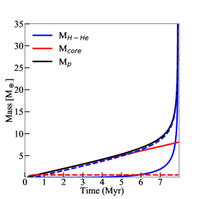
Figure 1: The envelope mass (blue), the core mass (red) and the total planetary mass (black) as a function of time. The solid accretion rate is set to be $10^{-6}$ M_⊕/yr. The dashed line corresponds to a case in which the heavy elements are deposited in the envelope (enriched) while the case of the solid line correspond to a non-enriched case in which all the heavy elements are assumed to reach the center (pure H-He envelope). The planetesimals are assumed to be composed of water with sizes of 10 m. More details about the two cases can be found in Venturini et al. (2016).

2.1 Capture Radius and Inferred Core Mass

At early stages, the planetesimals go through the envelope and reach the core, although some of their mass is deposited in the atmosphere. As time progresses, planetesimals no longer reach the center, and instead, their mass is deposited in the envelope, leading to envelope enrichment (Podolak et al., 1988; Mordasini et al., 2006; Fortney et al., 2013). The left panel of Figure 2 shows the capture radius $R_{cap}$ for different assumed planetesimal sizes and compositions. This plot demonstrates the importance of gas drag in determining the planet’s capture radius (and therefore the solid accretion rate). The importance of accounting for the ablated heavy-element mass in the atmosphere in planet formation models is reflected by the difference between the three curves. Small planetesimals have larger capture radii and are captured more easily. As expected, water planetesimals are captured more easily than rocky ones. The figure also shows that the planetesimal size, rather than composition, is the dominating parameter in determining the capture radius. The capture radius is determined by searching for the largest value of the impact parameter ($b_{crit}$) for which the planetesimal is captured (e.g., Helled et al. 2006). Further details on the capture radius are given in the Appendix.

The middle panel of Figure 2 shows the ratio between the heavy-element mass in the envelope ($M_{z,env}$) and the H-He mass. While the solid accretion rate is constant and equals to 10^-6 M_⊕/yr the accretion rate of H-He increases with time. As more H-He is accreted by the growing planet, $M_{z,env}$/$M_{H-He}$ decreases and finally the gas accretion rate exceeds that of the solids and the envelope’s metallicity decreases significantly. It is interesting to note that during the early stages, when the gaseous mass is still small, the peak of the heavy-element mass ratio ($M_{z,env}$/$M_{H-He}$) occurs at different times, and the exact value of $M_{z,env}$/$M_{H-He}$ depends on the assumed planetesimal size. Nevertheless, in all the cases, since the final envelope composition is dominated by the gas accretion, once the planet reaches Jupiter’s mass the envelope’s metallicity is found to be $Z\approx 0.01$. The exact value, however can change depending on whether planetesimals are expected to be accreted at later stages (see Helled & Lunine 2014).

As expected, ablation of planetesimals significantly changes the atmospheric mass, and larger planetesimals tend to reach the center and leading to less significant enrichment of the atmosphere. If heavy-element ablation is neglected the atmospheric mass is significantly smaller, which affects the subsequent planetary growth and the ablation of planetesimals at successive time step as well as the evolution of the atmosphere itself due to change in opacity and the envelope’s composition (equation of state). So far, this effect has only been considered by Venturini et al. 2016, and clearly, this effect is significant.

The inferred core mass for the different cases is presented in the right panel of Figure 2. We find that core growth occurs only at very early times (less than 1 Myrs) and that the core mass is rather small (less than 1.5 M_⊕). After that point the envelope is dense enough to ablate/fragment the accreted solids, and the heavy elements stop reaching the center keeping the core mass constant. The exact time at which the core stops growing and the final core mass depend on the properties of the envelope and the size and composition of the accreted planetesimals. However, in all cases the core stops growing early and its mass remains small. This confirms that the core accretion scenario can naturally lead to the formation of small cores, unless the accreted planetesimals are extremely large ($\gg$ 100 km). We find that when planetesimal ablation and fragmentation are included, the core mass is found to be small, and after a short time, for all the planetesimal sizes and compositions we consider, its mass reaches a maximum value in agreement with previous studies (Lozovsky et al. 2017, Brouwers et al. 2017). Indeed, it was found by Pollack et al. (1986) that, except for impactors with sizes larger than $1000$ km, the core mass stops increasing when it reaches a mass between $1$ and $2.8$ M_⊕. It should be noted, however, that during these formation phases there is no sharp boundary between the core and the envelope in terms of composition and the core region is not well defined (e.g., Helled & Stevenson 2017).

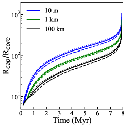
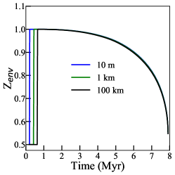
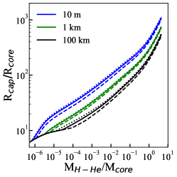
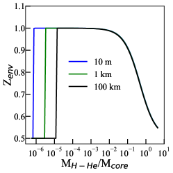
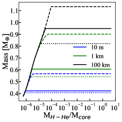
Figure 2: Left: Capture radius over core radius $R_{cap}/R_{core}$ for different planetesimal sizes. The dotted, solid, and dashed curves correspond to water, ice+rock, and rocky planetesimals, respectively. Middle: The envelope’s metallicity $Z_{env}$ vs. time for three different planetesimal sizes. The planetesimal composition is assumed to be water+rock. Right: Inferred core mass for the different cases. The dotted, solid, and dashed curves correspond to water, ice+rock, and rocky planetesimals, respectively. The top and bottom panels show the above properties vs. time and $M_{H-He}/M_{core}$, respectively.

3 The dominant mechanism: ablation or fragmentation?

While the result that once the core mass reaches a value of $\sim 1-2$ M_⊕ is robust, the actual distribution of the heavy elements in the envelope depends on whether the dominated mechanism is ablation (Equation 4) or fragmentation (Equation 2). Fragmentation often dominates the mass deposition of large planetesimal ($\geq$ 1 km) in the inner regions of the envelope, where both the planetesimal’s velocity and the atmospheric density are high. Small solids are mostly ablated and are typically deposited at higher regions in the envelope. Figure 3 shows the dominating mechanism for different planetesimal sizes and composition as the protoplanet grows. The larger the solids are, the more likely it is that they fragment since they are less affected by ablation (Mordasini et al., 2015). The planetesimal’s composition also plays an important role - water planetesimals have a lower material strength $\sigma$ comparison to rocky planetesimals, and can therefore fragment more easily.

Finally, the choice of the $C_{h}$ value is also important - the lower $C_{h}$ is the more likely it is that fragmentation occurs. This is because for low $C_{h}$ values ablation is less significant and planetesimal can reach deeper regions within the envelope where the density is high enough to cause fragmentation. In the case of big bodies the value of $C_{h}$ is expected to vary inversely proportional with the atmospheric density reaching value of $\sim 10^{-4}$, as can be seen adopting the formula given in Melosh & Goldin (2008) The prediction that the core mass remains small is insensitive to the dominating ”deposition mechanism”. In all cases after $\sim$1 Myr all the accreted solids are either ablated and fragmented and can no longer reach the core.

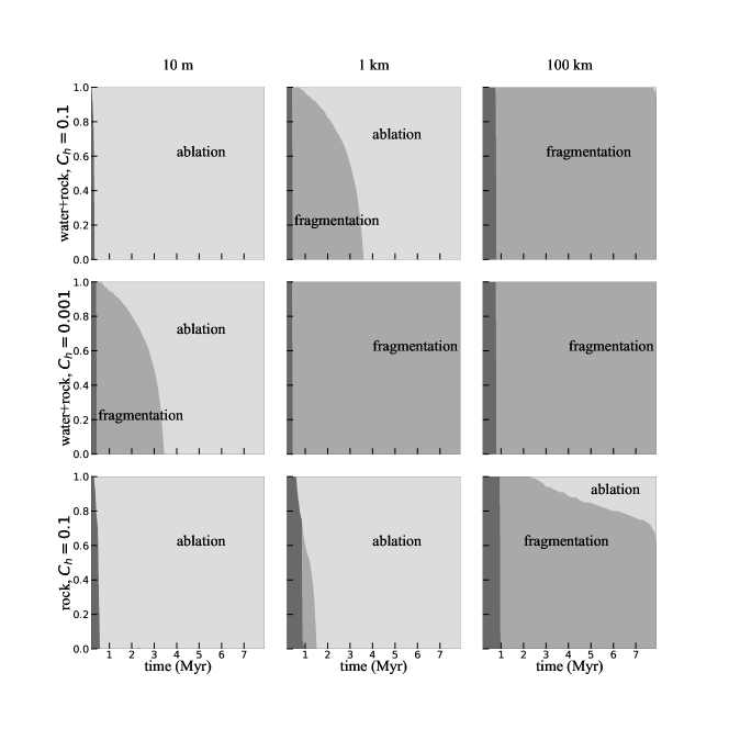
Figure 3: The fate of infalling planetesimals vs. time for different planetesimal properties and $C_{h}$ values. The different gray scales (from dark to light) correspond to the cases of reaching the core, fragmentation, and ablation, respectively. The $x$ axis shows the time, ranging from $0$ to $7$ Myr, while the $y$ axis shows the impact parameter of the planetesimal in unit of $b_{crit}$. The first column corresponds to 10m-sized planetesimals, while the second and third columns are for 1km-sized and 100km-sized planetesimals, respectively. The first row corresponds to a composition of water+rock, $C_{h}=0.1$, the second row is the same composition but with $C_{h}=0.001$, and the third row is for rocky planetesimals with $C_{h}=0.1$.

Figure 4 shows the inferred capture radius for different assumed $C_{h}$ (left panel) and $\epsilon$ (right panel) values for 1 km-sized planetesimals composed of water+rock. As expected, larger $C_{h}$ and $\epsilon$ values lead to more efficient capturing and larger capture radii. Interestingly, a change of $C_{h}$ and $\epsilon$ by several orders of magnitude results in a difference of up to a factor of two in the capture radius. Changing $C_{h}$ and/or $\epsilon$ leads to very similar results. This confirms that $R_{cap}$ is insensitive to ablation as noted by Inaba & Ikoma (2003). In addition, we show that $R_{cap}$ is nearly unchanged for $C_{h}$/$\epsilon$ values between 0.1 and $10^{-3}$. Only extremely low values can slightly change $R_{cap}$, but even then, the change is insignificant. This is because at such a low value ablation becomes completely negligible. However, as we show in the next section, the $C_{h}$ value has an important role in determining the heavy-element distribution in the planetary envelope.

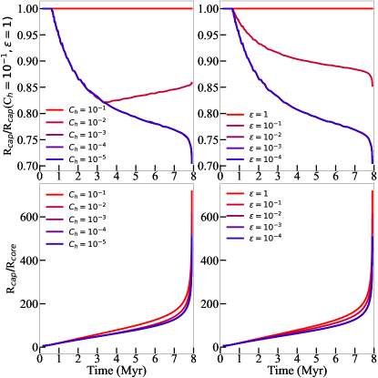
Figure 4: Top: $R_{cap}/R_{core}$ for different $C_{h}$ and $\epsilon$ values. Bottom: $R_{cap}/R_{cap}(C_{h}=0.1,\epsilon=1)$ for different $C_{h}$ and $\epsilon$ values. The planetesimals are assumed to be composed of water+rock and $1$ km in size.

4 The Distribution of Heavy Elements

Next, we present the predicted heavy-element distribution in the planetary envelope as a function of time for different model assumptions. We define $f_{Z,env}$ as the fraction of the accreted heavy-element mass per time-step deposited at a given region in the envelope. In order to derive $f_{Z,env}$ we calculate the heavy-element mass accreted by the protoplanet $M_{Z,acc}$ at a given time-step and follow the ablation of planetesimals in the envelope. For simplicity, the calculated $f_{Z,env}$ corresponds for a given time, and is not affected by the distribution calculated at a previous time-step. We can then find the fraction of the accreted mass of solids (per time-step) that is deposited at different depths. If all the planetesimals dissolve in the envelope, the integral of $f_{Z,env}$ over the planetary radius is equal to 1. At early stages when some planetesimals reach the core, the mass fraction of heavies that goes to the core is $1$ minus the integral. In the left panel of Figure 5 we compare the inferred $f_{Z,env}$ assuming $C_{h}=0.1$ for planetesimals composed of rock+ice with sizes of $10$ m and $100$ km. $f_{Z,env}$ is shown vs. normalized planetary radius. In both cases at very early times, the heavy elements are deposited near the center (core), then the small planetesimals quickly stop reaching the core and their mass is deposited in the envelope. This also occurs for large planetesimals but with a time lag of $\sim$ 1 - 2 Myr, for our specific formation model. 10 m-sized planetesimals enrich the outer part of the envelope and deposit most of their mass very far from the core, at normalized radius $0.7-0.8$. On the other hand, 100 km-sized planetesimals tend to enrich the inner parts of the envelope and most of their mass is deposited at a normalized radius of $\sim$ 0.2 - 0-3. In addition, $f_{Z,env}$ is found to be ”smoother” for the smaller planetesimals. In both cases as time progresses, and the envelope mass increases, the heavy elements are deposited in the upper parts of the envelope (towards a normalized radius of one).

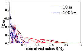
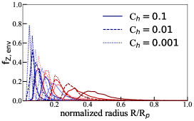
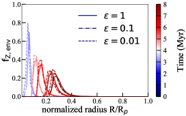
Figure 5: $f_{Z,env}$ vs. normalized radius at different times. The times are shown in the colour scale from red (10⁵ years, early) to blue ($8\times 10^{6}$ years, late). The plots are produced dividing the total radius of the planet in $50$ bins, each with a width of $0.02$ $R_{tot}$. These results are also presented in the Appendix where $f_{Z,env}$ at different times is shown in separate panels. Left: The solid and dashed lines correspond for planetesimals composed of a mixture of rock+ice with sizes of $10$ m and 100 km, respectively. Middle: Rocky 10 m-sized planetesimals with $C_{h}=0.1$ (solid), $C_{h}=0.01$ (dotted) and $C_{h}=0.001$ (dashed-dotted). Right: Rocky 1 km-sized planetesimals with different $\epsilon$ values. The solid, dashed and dotted stands for $\epsilon$ of 1, $0.1$ and $0.01$, respectively.

The sensitivity of $f_{Z,env}$ to the assumed $C_{h}$ value is shown in the middle panel of Figure 5. We find that for the 10 m-sized planetesimal changing the $C_{h}$ value leads to a significant change in $f_{Z,env}$. A smaller $C_{h}$ value leads to a distribution with a peak closer to the core. When using a small $C_{h}$ value ($10^{-4}$), even for the small planetesimals there is a negligible enrichment in heavy elements in the outer parts of the envelope. Since large planetesimals are less affected by ablation, the resulting $f_{Z,env}$ is less sensitive to the assumed $C_{h}$ value. In all the cases the heavy elements are deposited in the deep interior, leaving the outer envelope metal-poor. The inner regions are highly enriched mimicking a larger core. This configuration is consistent with a diluted core that is exact mass is not well-defined, due to the absence of a sharp boundary between it and the envelope (e.g. Lozovsky et al. 2017, Helled & Stevenson 2017, Wahl et al. 2017). It should be noted that for simplicity, we do not consider the re-distribution of heavies due to convective mixing (e.g. Lozovsky et al. 2017, Vazan et al. 2016, Venturini et al. 2016). If convection is efficient it would homogenize the gradient leading to a mixed envelope with a constant metallicity. Finally, in the right panel of Figure 5 we show the sensitivity of $f_{Z,env}$ to the assumed $\epsilon$ value. The trend is similar to the middle panel, but the dependence on $\epsilon$ is somewhat weaker implying that ablation is more important then radiation for these conditions. In the Appendix we present the results presented in Fig. 5 with $f_{Z,env}$ at different time in separate panels.

4.1 Different Fragmentation Models

When fragmentation occurs (Eq. 2), it does not necessarily imply an instantaneous deposition of the entire planetesimal’s mass at this location in the envelope. As discussed in Register et al. (2017) there are various ways to model fragmentation as listed below. A graphic representation of various fragmentation models is shown in Figure 6.

• Instantaneous: Deposition of all the fragmented material at the layer where fragmentation occurs. This is the simplest model for fragmentation.

• Single Bowl: The planetesimal fragments into two independent spherical bodies. Children bodies are assumed to be of equal mass, half of the parent’s mass and responds to gas drag independently (Mehta et al., 2017). The new size of the bodies is computed assuming that the same density as before fragmentation. The bodies continue to move (following Eq. 3) and lose mass due to ablation (Eq. 4) with the surface term being adjusted accordingly.

• Common Bowl: When fragmentation occurs, the parent body is split into two equally sized fragments, each with half the parents’ mass. The two fragments continue to interact with the gas being next to each other within a common bow shock, where the bodies present a common surface with respect to gas drag (Revelle, 2007, 2005). This implies that after fragmentation occurs the surface term in Eq. 3 is the sum of the surfaces of the two children bodies.

• Pancake Model: at the initial fragmentation point, the planetesimal is converted into a cloud of continuously fragmenting material that function aerodinamically as a single deforming body (Zahnle, 1992; Chyba et al., 1993; Hills & Goda, 1993). The cloud begins as a sphere and then flattens to get a pancake-like shape. The lateral spread is computed based on a dispersion velocity proportional to the square root of the envelope to planetesimal’s density ratio and the instantaneous velocity:

  $$v_{disp}=({7\rho_{gas}}/{2\rho_{p}})^{1/2}v,$$ (5)

  where $v$ is the impactor’s instantaneous velocity. The area of the pancake is then calculated per each time step $dt$ as

  $$A=\pi(r_{old}+v_{disp}dt)^{2}.$$ (6)

  The material continues to move towards the proto-planet’s centre following with the new surface $A$ given by Eq. 6. The drag coefficient calculated as in Podolak et al. (1988) neglecting the non-spherical shape of the object (Zahnle, 1992).

• Halved: When fragmentation occurs half of the mass is assumed to be deposited at the local layer while the rest of the mass planetesimal continues to travel towards the center with the same velocity that it had before it fragmented (Revelle, 2007, 2005).

(a)

(b)

(c)

(d)

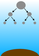
(e)

Figure 6: A graphic representation of the different fragmentation models: Instantaneous (a) Common Bowl (b), Halved (c), Pancake (d), and Single Bowl (e). More details on the fragmentation models can be found in (Register et al., 2017).

The material strength of the planetesimal is assumed to increase after fragmentation by the following power-law: $S_{c}=S_{p}(\frac{m_{p}}{m_{c}})^{\alpha}$ where $m_{c}$ and $m_{p}$ correspond to the mass of the child and parent, respectively, and $\alpha$ is a parameter between $0$ and $1$. Smaller fragments are assumed to have larger material strengths (Mehta et al., 2017; Artemieva et al., 2001; Weibull, 1951). The exact value of $\alpha$ is not well-determined because it depends on the inner structure of the planetesimal (both before and after fragmentation). In order to ensure that we do not bias the results, we run models with $\alpha$ values between $0$ and $1$ that are determined randomly, at each fragmentation.

The left panel of Figure 7 shows the inferred core mass using different fragmentation models and $C_{h}$ values. Since small planetesimals typically do not fragment we consider only the cases of 1 km and 100 km. We find that the simple ”instantaneous” fragmentation model leads to the smallest core mass, smaller than 1 M_⊕. Shortly after the point where the core stops growing in mass in the instantaneous fragmentation model, planetesimals fragment near the core (due to the small envelope mass). When fragmentation is included, the core mass can increase by $0.1-0.5$ M_⊕ within several thousand years. After that point even when fragmentation occurs the heavy elements are deposited too far from the core, and the core mass can no longer increase.

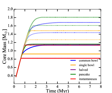
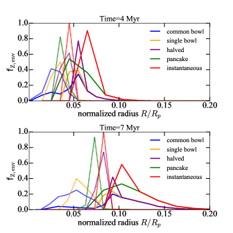
Figure 7: Left: Inferred core mass vs. time for the different fragmentation models. Solid and dashed-dotted lines are for 100 km-sized water planetesimals and $C_{h}=0.1$ and $C_{h}=10^{-3}$, respectively. The dashed lines correspond to 100 km-sized rocky planetesimals. Right: $f_{Z,env}$ vs. normalized radius up to 0.2 at 4 Myr and 7 Myr corresponding to a total planetary mass of $5$ and $15$ M_⊕, respectively.

Changing $C_{h}$ can also slightly increase the core mass when the other fragmentation models are considered. The ”halved” fragmentation model predicts a core mass similar or slightly larger than the simplest ”instantaneous” one, due to the rapid mass loss as more fragmentations occur. The largest core mass is obtained with the ”pancake” fragmentation model due to the increased size of the ”cloud” which travels towards the planetary center. Finally, similar core masses are predicted by ”common bowl” and ”single bow” fragmentation models. We conclude that the exact value of the predicted core mass weakly depends on the assumed fragmentation model, and is more affected by the assumed $C_{h}$ value.

Next, we investigate the sensitivity of $f_{Z,env}$ to the assumed fragmentation model. Since small planetesimals are ablated, it is the large planetesimals that are affected by the treatment of fragmentation and we therefore concentrate on the distribution for planetesimals sizes of 100 km. The results are presented in the right panel of Figure 7 at two different formation times: 4 Myr (top) and 7 Myr (bottom). These times correspond to a total mass (core + envelope) of $5$ and $15$ M_⊕, respectively. Note that we show the distribution up to a normalized radius of 0.2, since the distribution of heavy elements in outer regions is negligible since most of the material is deposited in the innermost regions. We find that $f_{Z,env}$ is relatively insensitive to the fragmentation model, but it does moderately affect the location of the peak and its spread.

5 A Semi-Analytical Approach to derive $f_{Z,env}$

In this section we present a semi-analytical approach to derive $f_{Z_{e}nv}$ in the planetary envelope. The equation of motion can be solved analytically neglecting the contribution of gas drag, providing a simple semi-analytical solution for $f_{Z,env}$ . This can be applied to large planetesimals ($\geq$ 1 km) which are less affected by gas drag (Equation 3). The equations can then be written as:

$$m_{pl}\frac{d\vec{v}}{dt}=-G\frac{M_{p}m_{pl}}{r^{3}}\vec{r},$$ (7)

$$\frac{dm_{pl}}{dt}=-\frac{A}{Q}\bigg{(}\frac{1}{2}C_{h}\rho_{gas}\left|v\right|^{3}+\epsilon\sigma T_{a}^{4}\bigg{)},$$ (8)

where the gas drag term in Equation 3 is neglected. The planetesimal’s velocity is a 2D vector that can be decomposed as

$$v=v_{r}\hat{r}+v_{\theta}\hat{\theta},$$ (9)

where $v_{r}={dr}/{dt}$ is the radial velocity and $v_{\theta}$ is the angular velocity given by $r({d\theta}/{dt})$, with $\theta$ being the polar angle.
Energy conservation implies:

$$v^{2}=v_{0}^{2}+2GM_{p}\bigg{(}\frac{1}{r}-\frac{1}{r_{0}}\bigg{)},$$ (10)

where $v_{0}$ is the initial planetesimal’s velocity and $r_{0}$ is its initial distance from the planet’s center. Angular momentum conservation implies:

$$v_{\theta}^{2}=\frac{L^{2}}{m_{pl}^{2}r^{2}},$$ (11)

where $L$ is the angular momentum, and the radial velocity is given by:

$$v_{r}^{2}=v^{2}-v_{\theta}^{2}.$$ (12)

Dividing both sides of Eq.8 by $v_{r}$ results in:

$$\frac{dm_{pl}}{dr}=-\frac{A}{Q}\bigg{(}C_{h}\frac{\rho_{gas}v^{3}}{2v_{r}(r)}+\epsilon\sigma T_{atm}^{4}\frac{1}{v_{r}(r)}\bigg{)},$$ (13)

where $v$ is given by Eq. 10 and $v_{r}$ by Eq. 12. Eq. 13 can also be written as:

$$\frac{dm_{pl}}{dr}=-f(r),$$ (14)

where ${dm_{pl}}/{dr}=-\frac{A}{Q}\bigg{(}C_{h}\frac{\rho_{gas}v^{3}}{2v_{r}(r)}+\epsilon\sigma T_{atm}^{4}\frac{1}{v_{r}(r)}\bigg{)}$. Finally, the planetesimal’s mass at a position $r$ within the envelope is given by

$$\int_{M_{0}}^{M(r)}dm=\int_{r_{0}}^{r}f(r)dr,$$ (15)

where $\rho$ and $T_{atm}$ are functions of $r$. The integration is performed up to M$(r)$ where $r$ is the location within the envelope where fragmentation occurs according to Equation (1). In order to estimate the total mass of heavy elements in the envelope one has to add the mass deposited due to fragmentation (the mass leftover after ablation).

We next integrate $f(r)$ numerically, starting from the core, simply using: $\int_{r_{core}}^{r_{max}}drf(r)$ where $dr$ is the size of an atmospheric shell and $f(r)$ is evaluated at the mid point in the atmospheric shell. The comparison between the numerical calculation and the analytical calculation is shown in Figure 8. As can be seen from the figure, the agreement is excellent. We therefore suggest that this approximation can be used to generate the heavy-element distribution in porotoplanetary atmospheres in different planet formation models, including planet population synthesis models (Mordasini et al. 2009, Benz et al. 2014).

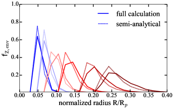
Figure 8: A comparison between the numerical (solid curve) and semi-analytical (dashed curve) model for the inferred $f_{Z,{env}}$ at different times. Shown are the results for planetesimals made of rock+ice with sizes of 1 km (left) and 100 km (right).

6 Discussion and Conclusions

Predicting the heavy-element distribution in giant planets is crucial for the characterization of Jupiter and Saturn as well as giant exoplanets. Today, when the atmospheric composition of exoplanets can be determined with spectroscopy measurements, the determination of the expected heavy-element distribution in the planets’ envelopes is vital to compare the measurements with theoretical predictions (e.g., Helled & Lunine 2014; Mordasini et al. 2016). The internal structure of giant protoplanes depends on the interaction of the solids with the gaseous envelope during the early formation stages. As we show here, the location in which the heavy elements are deposited depends on the planetesimals (solids) properties such as their size and composition, the fate of the accreted planetesimals (ablation/fragmentation) and other model assumptions.

We find that planetesimal fragmentation is important for planetesimal with sizes larger than 1 km, and that the importance of fragmentation vs. ablation is sensitive to the assumed $C_{h}$ value. Ablation typically results in a less-peaked distribution with enrichment of the outer regions of the envelope, while fragmentation enriches significantly the deep interior, leaving the outer envelope metal-poor. Finally, we present a semi-analytical prescription for determining the heavy-element distribution in the envelope. This can be easily implemented in giant planet formation calculation and can be used to include the presence of the heavy-elements in a more consistent manner, i.e., accounting for their effect on the EOS and opacity calculation.

Although different model assumptions lead to different heavy-element distributions, we find that in all the cases heavy elements stop reaching the core once it reaches a mass of 0.5-2 M_⊕. For our specific Jupiter formation model this corresponds to a time of 2 Myr. While the results presented in the paper such as the value of the maximum core mass, and the shape of the heavy-element distribution depend on the assumed atmospheric model and growth history, the general trend of the core reaching a maximum mass, and that most of the accreted heavy-elements are deposited in the envelope is robust and is in agreement with previous studies (Lozovsky et al., 2017; Brouwers et al., 2017; Venturini et al., 2016; Mordasini et al., 2015; Iaroslavitz & Podolak, 2007).

It should be noted, however, that although the core mass is found to be very small, the inner region can still be highly enriched with heavy elements (nearly pure heavies). In that case the density profile is not very different from that of a larger core, and this configuration can be viewed as a diluted/fuzzy core (Lozovsky et al., 2017; Helled & Stevenson, 2017; Wahl et al., 2017). The core mass can slightly increase when fragments are allowed to reach the core but only by up to 0.5 M_⊕. Also in this case the core mass does not exceed $\sim$2 M_⊕. We also show that dissolution of planetesimals in the envelope can increase the atmospheric mass (and its mean molecular weight) by a large factor.

It is interesting to note that our study confirms the assumption of Venturini et al. 2016 that envelope enrichment begins once the core masses reaches a few Earth masses. While the exact number depends on the specific formation model and planetesimal properties, it supports the emerging picture that giant planets formed by core accretion are likely to have small cores and that envelope enrichment cannot be neglected. This work only explore the sensitivity of the inferred heavy-element distribution to different model assumptions. This is only the first step, and clearly more work is required. Future studies should also investigate the mixing of heavy elements at early stages to determine the expected structure of the envelope (homogenous vs. compositional gradients) and model the planetary growth in a self-consistent manner in which envelope enrichment is considered and is linked to the expected distribution of the heavy elements. Accounting for the heavy-element distribution and their effect on the planetary growth and long-term evolution can improve our understanding of giant planet formation and of the connection between the current-state structure and planetary origin.

Planetesimal-Atmosphere Interaction

The planetesimal dissolution is derived by following in detail the planetesimal’s trajectory within the planetary envelope. The planetesimal’s impact parameter is defined as the distance on the $y$-axis between the initial point of the trajectory and the planet’s center. The maximum impact parameter that leads to planetesimal capture is defined as the critical impact parameter $b_{crit}$. The value of $b_{crit}$ changes with the physical properties of the atmosphere (e.g., mass, pressure, temperature) and the planetesimal (e.g., size, composition). A planetesimal (with the same size and composition) with an impact parameter larger than $b_{crit}$ escapes the planet and cannot be accreted. Planetesimal escape is defined to occur when the planetesimal’s kinetic energy is slightly greater than the gravitational one as defined by Pollack et al. (1996). The planetary capture radius $R_{cap}$ is defined as the closest distance to the planet’s center for an impact parameter slightly great than $b_{crit}$ Helled et al. (2006). Figure 9 presents a graphic representation of $b_{crit}$ and $R_{cap}$.

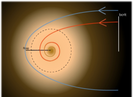
Figure 9: A graphic representation of the planetesimal-envelope interaction.

In Figure 10 we compare our inferred $R_{cap}$ with the semi-analytical formula of Inaba & Ikoma (2003). As can be seen from the figure, there is a very good agreement.

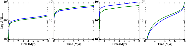
Figure 10: A comparison of the inferred $R_{cap}$ using our numerical calculation (blue line) with the semi-analytical formula of Inaba & Ikoma (2003) (green line) for four different formation models. Left, middle left and middle right panels correspond to models with a surface solid density of $10$ $g/cm^{2}$ and planetesimal sizes of $100$ km, $1$ km, and $10$ m, respectively. Right: the formation model used in this work with $100$ km-sized planetesimals.

The Distribution of Impact Parameters

In order to infer the heavy-element distribution we distribute $100$ planetesimals with impact parameters between zero and $b_{crit}$. Planetesimals with large impact parameters tend to spend more time in the outer part of the envelope and to experience gas drag and ablation before they are captured. On the other hand, planetesimals with small impact parameters can penetrate deeper in the atmosphere and reach closer to the core. We investigate the sensitivity of the inferred heavy-element distribution in the planetary atmosphere on the assumed impact parameter distribution. We consider two cases. In the first case we assume that the planetesimals are uniformly distributed along the z-axis (uniform) while in the second one we assume a gaussian distribution for the impact parameters picking at the disk’s mid-plane (planetary equator). The width of the gaussian distribution is set to be time dependent ranging from 0.5 to 0.1 of the disk’s height, which is taken to be the ratio between the sound speed and the Keplerian velocity. Such a distribution is more realistic since the concentration of planetesimals is expected to increase toward the disk’s midplane. A comparison of the inferred $f_{Z,env}$ assuming uniform and gaussian planetesimal distribution is presented in Figure 11. We find that the gaussian distribution results in a slightly higher concentration of planetesimals in the deep interior. This is an expected result because in that case there is a larger number of planetesimals at the disk’s mid-plane that can reach the central regions. However, despite this difference, the two curves are similar and differ by only up to 5-10%. We therefore conclude that for the purpose of calculating the heavy-element distribution in protoplanets assuming a uniform distribution is sufficient.

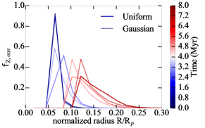
Figure 11: $f_{Z,env}$ at different times using two different distribution of planetesimals along the planet’s feeding zone. The solid line correspond to a uniform distribution while the dotted line for a gaussian distribution picked at the mid-plane. The planetesimals are assumed to be pure rocky and 100 km in size.

The Importance of Settling

When heavy elements dissolve in the envelope they are assumed to be fully vaporized. Then, the amount of heavy elements that remains at a given location within the envelope is determined by the local temperature and its vapor pressure $P_{vap}$. In order to calculate how much of the ablated mass remains in the given shell we follow the procedure presented in Iaroslavitz & Podolak (2007) and assume that the entire ablated mass is initially in the vapor phase, and then compare the partial pressure $P_{par}$ of the vapor to the saturation vapor pressure at the ambient temperature. If $P_{par}>P_{vap}$, the abundance of the volatile mass in the gas phase is such that $P_{par}=P_{vap}$, and any excess of material settles to the layer below.

In computing the vapor pressure we assume that the vapor obeys the ideal gas law. The expressions for the vapor pressure are $P_{vap}^{ice}=e^{-5640.34/T+28.867}$ and $P_{vap}^{rock}=10^{-24605/T+13.176}$ (see Iaroslavitz & Podolak (2007); Lozovsky et al. (2017) for details). In this approach, it is assumed that unlimited amount of heavy-element material can be kept in the vapor phase in regions where the temperature exceeds the critical point. The critical temperature can be derived from experimental data and are taken to be 567.3 K for H₂O and 4000 K for rock.

At each timestep we begin from the outermost layer and follow the material that settles to the core. Figure 12 shows the mass that is expected to be added to the core via settling. We find that the mass joining the core due to settling is very limited and can be neglected. This result, however, is linked to the assumption that hot enough (above the critical temperature) regions can absorb the heavy-elements. Future studies should include the formation of clouds and follow the settling of elements at the critical point in order to provide more robust conclusions on the importance of settling inside giant protoplanets.

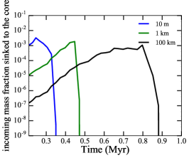
Figure 12: Mass added to the core by settling for planetesimals made of water+rock. We consider three different planetesimal sizes: 10 m (blue), 1 km (green) and 100 km (black).

A different representation of $f_{Z,env}$

Below we the results of Fig. 5 for $f_{Z,env}$ when the various times are presented in separate panels. The left panel of figure 13 shows $f_{Z,env}$ when assuming rock + water planetesimals with different sizes. It can be seen that larger planetesimals tend to enrich the inner part of the envelope, while small planetesimals deposit their mass in the outer regions. In the right panel of figure we present $f_{Z,env}$ for different assumed $C_{h}$ values. As expected, a smaller $C_{h}$ value leads to a distribution with the peak being closer to the center.

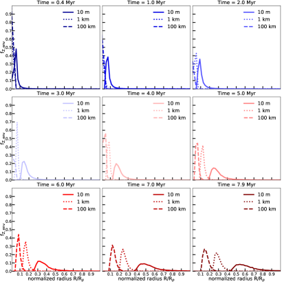
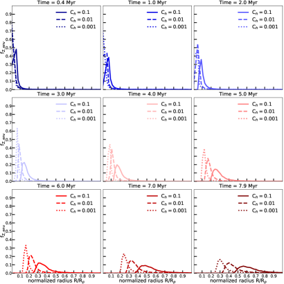
Figure 13: $f_{Z,env}$ in the planetary envelope vs. normalized radius at different times. The times are shown in different panels. Left: Results for different planetesimal sizes. The solid, dotted and dashed lines correspond for planetesimals with sizes of $10$ m, $1$ km and $100$ km, respectively. Right: Results for different assumed $C_{h}$ values. The solid, dashed and dotted lines correspond for planetesimals with a $C_{h}$ value of $0.01$ and $0.001$, respectively. The planetesimals are assumed to be made of rock and be $10$ m in size.

References

- Alibert (2017) Alibert, Y., 2017, A&A, 606, A69
- Alibert et al. (2005) Alibert, Y., Mordasini, C., Benz, W., & Winisdoerffer, C. 2005, A&A, 434, 343
- Allen, H. J. (1962) Allen, H. J., 1962, NASA SP-24.
- Apstein et al. (1989) Apstein, E. Z., Pilyugin N. N. P. S., Evastianenko V.G., G.A. Tirsky 1989, Itogi Nauki Tekh. Mekh. Zhidkosti Gasa, 23, 116–236.
- Artemieva et al. (2001) Artemieva, N.A., Shuvalov, V.V. 1996, Shock Waves, 5(6), 359-367
- Baraffe et al. (2006) Baraffe, I., Alibert,Y., Chabrier, G.,Benz, W. , 2006, A&A, 450, 1221-1229
- Benz et al. (2014) Benz, W., Ida, S., Alibert, Y., Lin, D., Mordasini, C., 2014, Protostars and planets VI
- Bodenheimer & Lissauer (2014) Bodenheimer, P. & Lissauer, J. J., 2014, ApJ, 791, 103
- Bodenheimer & Pollack (1986) Bodenheimer, P. & Pollack, J. B., 1986, Icarus, 67, 391
- Brouwers et al. (2017) Brouwers, M. G., A. Vazan, C. W. Ormel, 2017, Astronomy and Astrophysics, Forthcoming article
- Chyba et al. (1993) Chyba, C. F., Thomas, P. J., Zahnle, K. J., 1993, Nature 361, 40-44
- Fortney et al. (2013) Fortney, J. J., Mordasini, C., Nettelmann, N., Kempton, E., Greene, T., Zahnle, K., 2013, ApJ, 775, 1
- Freedman et al. (2014) Freedman, R. S., Lustig-Yaeger, J., Fortney, J. J, et al. 2014, ApJS, 214, 25
- Hayashi (1981) Hayashi, C., 1981, Progress of Theoretical Physics Supplement, 70, 35
- Helled et al. (2011) Helled, R., Anderson, J. D., Podolak, M., Schubert, G., 2011, ApJ, 726, 15
- Helled & Bodenheimer (2014) Helled, R., & Bodenheimer, P., 2014, ApJ, 789, 69
- Helled & Lunine (2014) Helled, R., Lunine, J., 2014, Monthly Notices of the Royal Astronomical Society, 441(3)
- Helled et al. (2014) Helled, R. et al., 2014, Protostars and Planets VI, 643
- Helled & Stevenson (2017) Helled, R., Stevenson David, 2017, ApJ, 840, 1
- Helled et al. (2006) Helled, R., Podolack, M., Kovetz, A., 2006, Icarus, 185, 1
- Hills & Goda (1993) Hills, J. G., Goda, M. P., 1993, AJ, 105, 3
- Hori & Ikoma (2011) Hori, Y. & Ikoma, M., 2011, MNRAS, 416, 1419
- Iaroslavitz & Podolak (2007) Iaroslavitz, E. & Podolak, M., 2007, Icarus, 187, 600
- Ida & Makino (1993) Ida, S. & Makino, J., 1993, Icarus, 106, 210
- Ikoma & Hori (2012) Ikoma, M. & Hori, Y., 2012, ApJ, 753, 66
- Inaba & Ikoma (2003) Inaba, S. & Ikoma, M., 2003, A&A, 410, 711
- Lozovsky et al. (2017) Lozovsky, M., Helled, R., Rosenberg, E. D., Bodenheimer, P., 2017, ApJ, 836, 227
- Makinde et al. (2013) Makinde, O.D., Khan, W.A., Khan, Z.H., 2013, International Journal of Heat and Mass Transfer 62, 526-533
- Mehta et al. (2017) Mehta, P. M., Minisci, E. M., Vasile, M., 2017, 4th IAA PDC
- Melosh & Goldin (2008) Melosh, H. J., Goldin, T. J., 2008, in Lunar and Planetary Science Conference
- Mordasini (2014) Mordasini, C. 2014, A&A, 572, A118
- Mordasini et al. (2006) Mordasini, C., Alibert, Y. & Benz, W., 2006, in Tenth Anniversary of 51 Peg-b: Status of and prospects for hot Jupiter studies, ed. L. Arnold, F. Bouchy & C. Moutou, 84
- Mordasini et al. (2015) Mordasini, C., Mollière, P., Dittkrist, Jin, K., M.,Alibert, Y, 2015, International Journal of Astrobiology, 14
- Mordasini et al. (2009) Mordasini, C., Alibert, Y., Benz, W., 2009, A&A, 501, 3, July III
- Mordasini et al. (2016) Mordasini, C., Boekel, R., Mollière, P., Henning, Th., Benneke, B., 2016, ApJ, 832, 1
- Movshovitz et al. (2010) Movshovitz, N., Bodenheimer, P., Podolak, M., Lissauer, J. J., 2010, Icarus, 209, 616
- Movshovitz & Podolak (2008) Movshovitz, N. & Podolak, M., 2008, Icarus, 194, 368
- Nijemeisland & Dixon (2004) Nijemeisland, M. & Dixon, A. G., 2004, AIChE J., 50, 906-921.
- Register et al. (2017) Register, J. P., Mathias, D. L.,Wheeler, L. F. 2017 Icarus, 284, 157–166.
- Perri & Cameron (1974) Perri, F., Cameron, A. G. W., 1974, Icarus, 22, 416
- Pinhas et al. (2016) Pinhas, A., Madhusudhan, N., Clarke, C., 2016, MNRAS, 463, 4, 21, 4516–4532
- Pletcher et al. (2012) Pletcher, R. H., Tannehill, J. C., Anderson, D., 2012, Computational fluid mechanics and heat transfer, third edition
- Podolak (2003) Podolak, M. 2003, Icarus, 165, 428
- Podolak et al. (1988) Podolak, M., Pollack, J. B., Reynolds, R. T., 1988, Icarus, 73, 163
- Pollack et al. (1996) Pollack, J. B., Hubickyj, O., Bodenheimer, P., Lissauer, J. J., Podolak, M., Greenzweig, Y., 1996, Icarus, 124, 62
- Pollack et al. (1986) Pollack, J. B., Podolak, M., Bodenheimer, P., Christofferson, B. 1986, Icarus, 67, 3
- Revelle (2005) Revelle, D. O., 2005, Earth, Moon, and Planets 95: 441-476
- Revelle (2007) Revelle, D. O., 2007, Near Earth objects, our celestial neighbors: Opportunity and risk, 95-106
- Saumon et al. (2015) Saumon, D., Chabrier, G., van Horn, H. M., 1995, ApJS, 99, 713
- Svetsov et al. (1995) Svetsov , V. V.,Nemtchinov, I. V.,Teterv, A. V., 1995, Icarus, 116, 131–153.
- Vazan et al. (2018) Vazan, A.,Helled, R. , Guillot, T., 2018, A&A, 610, L14
- Vazan et al. (2016) Vazan, A., Helled, R., Podolak, M.,Kovetz, A., 2016, ApJ, 829, 2
- Venturini et al. (2016) Venturini, J., Alibert, Y., Benz, W., 2016, A&A, 596, A90
- Venturini et al. (2015) Venturini, J., Alibert, Y., Benz, W.,Ikoma, M., 2015, A&A, 576, A114
- Wahl et al. (2017) Wahl et al., 2017, Geophys. Res. Lett. 44, 4649–4659
- Weibull (1951) Weibull, 1951, Appl. Mech., 10, 140-147
- Wuchterl, G. (1993) Wuchterl, G., 1993, Icarus, 106, 323
- Zahnle (1992) Zahnle, K., J., 1992, JGR, 97, 10243