Gravitational waves and collider signatures from holographic phase transitions in soft walls

Abstract:

Using a five-dimensional warped model including a scalar potential with an exponential behavior in the infrared, and strong back-reaction over the metric, we study the electroweak phase transition, and explore parameter regions that were previously inaccessible. The model exhibits gravitational waves and predicts a stochastic gravitational wave background observable, both at the Laser Interferometer Space Antenna and at the Einstein Telescope. Moreover, concerning the collider signatures predictions, the radion evades current constraints but may show up in future LHC runs.

1 Introduction

The Standard Model (SM) of particle physics fails to explain a number of observational and theoretical issues, such as the baryon asymmetry of the universe, the origin of inflation and the strong sensitivity to high scale physics. The latter problem is commonly known as the hierarchy problem, and has motivated the study of several Beyond the SM (BSM) scenarios. One of the most fruitful BSM frameworks is the Randall-Sundrum model [1]. In this scenario the hierarchy between the Planck and the ElectroWeak (EW) scale is generated by a warped extra dimension in Anti de Sitter (AdS) space. This model contains a light state, the radion, which is dual to the dilaton, a Goldstone boson of the conformal invariance of the dual four-dimensional (4D) theory, and it is typically the lightest BSM state. The radion undergoes a ’holographic’ first order phase transition during which it acquires a vacuum expectation value [2, 3]. Models with small back-reaction on the gravitational metric suffer from perturbativity problems of the five-dimensional (5D) gravitational theory. In the present work we will introduce a method to deal with large back-reaction issues, that generalizes the superpotential procedure. For concreteness we will focus on a class of theories where the conformal symmetry is strongly broken in the infrared (IR). This kind of models were also considered to study EW precision data [4, 5], and most recently the B-meson anomalies [6, 7, 8].

2 The radion effective potential

In this section we present the model, and develop a novel method to employ the superpotential formalism to compute the effective potential at zero and finite temperature without major problems with the back-reaction. We consider a scalar-gravity system with two branes at values $r=r_{0}$ (UV brane), and $r=r_{1}$ (IR brane). The 5D action of the model reads

$$S = \int d^{5}x\sqrt{|\det g_{MN}|}\left[-\frac{1}{2\kappa^{2}}R+\frac{1}{2}g^{MN}(\partial_{M}\phi)(\partial_{N}\phi)-V(\phi)\right]$$ (1)

$$\qquad-\sum_{\alpha}\int_{B_{\alpha}}d^{4}x\sqrt{|\det\bar{g}_{\mu\nu}|}\Lambda_{\alpha}(\phi)-\frac{1}{\kappa^{2}}\sum_{\alpha}\int_{B_{\alpha}}d^{4}x\sqrt{|\det\bar{g}_{\mu\nu}|}K_{\alpha}\,.$$

There are three kind of contributions to the action corresponding to the bulk, the brane and the Gibbons-Hawking-York contribution. $V(\phi)$ is the bulk potential, $\Lambda_{\alpha}(\phi)\;(\alpha=0,1)$ are the UV and IR 4D brane potentials at $(\phi(r_{0}),\phi(r_{1}))$, and $\kappa^{2}=1/(2M^{3})$ with $M$ being the 5D Planck scale. The metric is defined in proper coordinates as $ds^{2}=\bar{g}_{\mu\nu}dx^{\mu}dx^{\nu}-dr^{2}$ with $\bar{g}_{\mu\nu}=e^{-2A(r)}\eta_{\mu\nu}$ the 4D induced metric on the branes. In order to solve the hierarchy problem, the brane dynamics should fix $(\phi_{0},\phi_{1})$ to get $A(\phi_{1})-A(\phi_{0})\approx 35$, and this implies $M_{{\textrm{Planck}}}\simeq 10^{15}M_{\textrm{TeV}}$. We have introduced a superpotential, whose relation with the scalar potential is $V(\phi)=\frac{1}{8}W^{\prime}(\phi)^{2}-\frac{\kappa^{2}}{6}W^{2}(\phi)$.

2.1 The effective potential

By using the equations of motion of the model, the action (1) can be written as [9]

$$S=-\int d^{4}x\,V_{\textrm{eff}}\,,\qquad\textrm{where}\qquad V_{\textrm{eff}}=\left[e^{-4A}\left(W+\Lambda_{1}\right)\right]_{r_{1}}+\left[e^{-4A}\left(-W+\Lambda_{0}\right)\right]_{r_{0}}\,.$$ (2)

After fixing $r_{0}=0$, the variable $r_{1}$ turns out to be the brane distance. The equation of the superpotential is a first order differential equation, so that it admits an integration constant that we will denote by $s$. If $W_{0}$ is a particular solution of the equation of motion with potential $V$, then it is possible to find a general solution of the equation as an expansion of the form $W=\sum_{n=0}^{\infty}s^{n}W_{n}$, where $W_{n}$ can be computed iteratively from $W_{0}$. An explicit solution for $n=1$ is given by [10, 11]

$$W_{1}(\phi)=\frac{1}{\ell\kappa^{2}}\exp\left(\frac{4\kappa^{2}}{3}\int_{v_{0}}^{\phi}\frac{W_{0}(\bar{\phi})}{W^{\prime}_{0}(\bar{\phi})}d\bar{\phi}\right)\,,$$ (3)

where $\ell$ is the AdS radius. We can similarly expand the scalar field as $\phi(r)=\phi_{0}(r)+s\,\phi_{1}(r)+\mathcal{O}(s^{2})$. The integration constant, $s$, is fixed by the boundary condition $\phi(r_{1})=v_{1}$, leading to $s(r_{1})=(v_{1}-\phi_{0}(r_{1}))/\phi_{1}(r_{1})$. Therefore the superpotential acquires an explicit dependence on the brane distance, $W(v_{\alpha})=W_{0}(v_{\alpha})+s(r_{1})W_{1}(v_{\alpha})+\cdots$, which in turn creates a non-trivial dependence on $r_{1}$ of the effective potential of Eq. (2). We will use this formalism for a kind of soft-wall phenomenological models defined by the superpotential $W_{0}(\phi)=\frac{6}{\ell\kappa^{2}}\left(1+e^{\gamma\phi}\right)$ and concentrate in several benchmark scenarios, covering parameter configurations with large and small back-reactions on the metric. In particular: i) Scenario A (small back-reaction), $\kappa^{2}=\frac{1}{4}\ell^{3}$; ii) Scenario B (large back-reaction), $\kappa^{2}=\frac{1}{4}\ell^{3}$; and iii) Scenario C (large back-reaction), $\kappa^{2}=\ell^{3}$ (cf. Ref. [9] for details). Table 1 shows the radion mass obtained in each scenario by using the approximate mass formula of Ref. [5]. Using this technique we find, for scenario B, the effective potential of Fig. 1 (left).

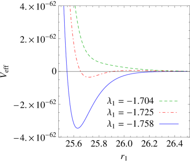
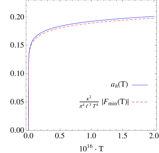
Figure 1: Left panel: Effective potential for different values of $\lambda_{1}$ in units of $\ell$. Right panel: $a_{h}(T)$ (blue solid line) and $\kappa^{2}|F_{\rm min}|/(\pi^{4}\ell^{3}T^{4})$ (red dashed line) as a function of $T$. We rescale the brane tensions as $\lambda_{\alpha}=\frac{\ell\kappa^{2}}{6}\Lambda_{\alpha}$. In both panels we have considered the ’large back-reaction scenario B’.

Scen.	$\lambda_{1}$	$m_{\textrm{rad}}/{\textrm{GeV}}$	$T_{c}/{\textrm{GeV}}$	$T_{n}/{\textrm{GeV}}$	$T_{R}/{\textrm{GeV}}$	$\alpha$	$\log_{10}(\beta/H_{\star})$
A	-1.250	199.8	230	-	-	-	-
B1	red-2.583	915	633	328	821.8	4.61	1.99
B2	blue-2.125	745	463	26	566.4	$4.0\cdot 10^{4}$	1.23
C	red-3.462	477	252	112	133.7	5.0	1.05

Table 1: List of benchmark scenarios considered in this work. The outputs obtained in each scenario are presented from the third column on. The foreground redred [blueblue] color on the value of $\lambda_{1}$ indicates that the corresponding phase transition is driven by $O(3)$ [$O(4)$] symmetric bounce solutions, cf. Sec. 3.1.

2.2 The effective potential at finite temperature

In the AdS/CFT correspondence a black hole (BH) solution describes the high temperature phase where the dilaton is in the symmetric phase, i.e. $\langle\mu\rangle=0$.  Let us consider the BH metric

$$ds_{{\textrm{BH}}}^{2}=-h(r)^{-1}dr^{2}+e^{-2A(r)}(h(r)dt^{2}-d\vec{x}^{\,2})\,,$$ (4)

where the blackening factor vanishes at the event horizon, i.e. $h(r_{h})=0$. The equations of motion of the system reduce to three independent equations with five integration constants, which can be fixed by imposing boundary conditions at the UV brane, $r=0$, and regularity conditions at the horizon, $r=r_{h}$. Then, the temperature and entropy of the BH can be expressed as

$$T_{h}=\frac{1}{4\pi}e^{-A(r_{h})}\big{|}h^{\prime}(r)\big{|}_{r=r_{h}}\,,\qquad S=\frac{4\pi}{\kappa^{2}}e^{-3A(r_{h})}\equiv\frac{4\pi^{4}\ell^{3}}{\kappa^{2}}a_{h}(T_{h})T_{h}^{3}\,,$$ (5)

where $a_{h}(T)$ is a smooth function which measures the deviation from the conformal limit, being $a_{h}=1$ the conformal solution. Finally, the free energy of the system has a minimum at $T_{h}=T$, which can be approximated by $F_{{\textrm{min}}}(T)\simeq-\frac{\pi^{4}\ell^{3}}{\kappa^{2}}a_{h}(T)T^{4}$. The numerical result of this procedure within scenario B is shown in Fig. 1 (right). For small back-reaction $a_{h}(T)$ basically reproduces the case of pure AdS ($a_{h}=1$), whereas for large back-reaction the value is $a_{h}(T)\ll 1$. This effect strongly influences the nucleation temperature of the phase transition. We find from our numerics that the behavior of $a_{h}(T)$ is generic and only depends on the amount of back-reaction.

3 The phase transition

In this section we study the phase transition mechanism of the radion as well as its implications for the EW phase transition.

3.1 The dilaton phase transition

When considering the system at finite temperature, there are two competing phases: the BH deconfined phase and the soft-wall confined phase, characterized by $\langle\mu\rangle=0$ and $\langle\mu\rangle\neq 0$, respectively. The free energies of these phases are

$$F_{\rm{deconfined}}(T)=E_{0}+F_{{\textrm{min}}}(T)-\frac{\pi^{2}}{90}g_{d}^{{\textrm{eff}}}T^{4}\,,\qquad F_{\rm{confined}}(T)=-\frac{\pi^{2}}{90}g_{c}^{{\textrm{eff}}}T^{4}\,,$$ (6)

where $E_{0}\equiv V_{{\textrm{eff}}}(\mu=0)-V_{{\textrm{eff}}}(\mu=\langle\mu\rangle)>0$, while $g_{c(d)}^{{\textrm{eff}}}$ are the effective degrees of freedom in the confined (deconfined) phase. When the temperature is decreasing, the critical temperature at which the phase transition starts being allowed is given by $F_{\rm{deconfined}}(T_{c})=F_{\rm{confined}}(T_{c})$. The phase transition happens when the barrier between the false BH minimum and the true vacuum is overcome. While at high $T$ this process is driven by thermal fluctuations and the corresponding Euclidean action is $O(3)$ symmetric, at low $T$ the transition can occur via quantum fluctuations with an $O(4)$-symmetric action. The corresponding equation of motion of the radion field is known as the ‘bounce equation’ and, for the $O(n)$ symmetric Euclidean action, it is written as [12] 

$$\frac{\partial^{2}\mu}{\partial\rho^{2}}+\frac{(n-1)}{\rho}\frac{\partial\mu}{\partial\rho}-\frac{\partial V_{{\textrm{eff}}}}{\partial\mu}=0\,,\qquad\textrm{with}\qquad\frac{1}{2}\mu^{\prime\,2}(\rho)\big{|}_{\mu=0}=\left|F_{{\textrm{min}}}(T)\right|\,.$$ (7)

The bubble nucleation rate from the false BH minimum to the true vacuum per Hubble volume $\mathcal{V}$ is $\Gamma/\mathcal{V}\simeq e^{-S_{E}}\simeq e^{-S_{3}/T}+e^{-S_{4}}$, so that it is dominated by the least action. Nucleation happens when the probability for a single bubble to be nucleated within one horizon volume is ${\cal O}(1)$, which corresponds to $S_{E}\lesssim 4\log\left(M_{{\textrm{Planck}}}/\langle\mu\rangle\right)\approx 140$ [13]. Fig. 2 (left) shows the numerical result in a scenario with large back-reaction (B₁). For large (small) values of $|\lambda_{1}|$ the phase transition is dominated by the $O(3)(O(4))$ bounce. When the back-reaction is small neither $S_{4}$ nor $S_{3}/T$ reach the upper bound.

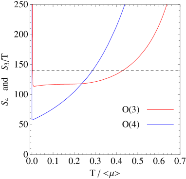
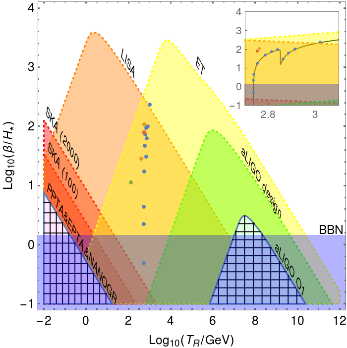
Figure 2: Left panel: $S_{4}$ and $S_{3}/T$ as a function of temperature (normalized to $\langle\mu\rangle$). We have considered scenario B₁. Right panel: The $T_{R}-\beta/H_{\star}$ parameter space that exhibits SNR $>10$ at SKA, LISA, aLIGO, and ET [14, 15, 16, 17]. The Big Bang nucleosynthesis bound excludes the blue area. It is displayed as dots the values obtained in several benchmark scenarios: B (blue points), C (green point) and other scenarios discussed in Ref. [9]. The inserted figure is a zoom of the main one in the regime of the model prediction.

On the other hand, inflation starts when $E_{0}$ dominates the value of the energy density, i.e. $\rho_{\rm{deconfined}}(T_{i})\simeq E_{0}$, and it finishes when bubbles percolate at $T\simeq T_{n}$. Finally, one can assume that during the phase transition the energy density is approximately conserved, so that at the end of the transition the universe ends up in the confined phase at the reheating temperature $T_{R}$ given by $\rho_{\rm{confined}}(T_{R})=\rho_{\rm{deconfined}}(T_{n})$. In Table 1 we summarize the values of these observables.

3.2 The electroweak phase transition

When $T$ decreases and the BH moves beyond the IR brane, the Higgs field $H$, localized nearby the IR brane, appears. Then the effective potential becomes a function of the radion and the Higgs [3]:

$$V(\mu,H)=V_{{\textrm{eff}}}(\mu)+\left(\frac{\mu}{\langle\mu\rangle}\right)^{4}V_{{\textrm{SM}}}(H,T)\,,\quad\textrm{with}\quad V_{{\textrm{SM}}}(H,T)=-\frac{1}{2}m^{2}H^{2}+\frac{\lambda}{4}H^{4}+\Delta V_{{\textrm{SM}}}(H,T)\,.$$ (8)

Here the Higgs mass is $m_{H}^{2}=2\lambda v^{2}\simeq(125\,{\textrm{GeV}})^{2}$ with $v=246\,{\textrm{GeV}}$, and $\Delta V_{\rm SM}(H,T)$ contains loop corrections. $V_{\rm SM}(H,T)$ has its absolute minimum at $\langle H(T)\rangle=v(T)$ which, at leading approximation for the thermal corrections, turns out to be

$$v(T)=\left\{\begin{tabular}[]{cl}0&for $T>T_{{\textrm{EW}}}$\\ $v\sqrt{1-T^{2}/T^{2}_{{\textrm{EW}}}}$&for $T\leq T_{{\textrm{EW}}}$\end{tabular}\right.$$ (9)

with $T_{{\textrm{EW}}}\simeq 150\,{\textrm{GeV}}$. The relevant quantity to study, when the universe ends up in the EW broken phase after the bubble percolation, is the reheating temperature. In scenarios with $T_{R}>T_{{\textrm{EW}}}$, at the end of the reheating process the Higgs field is in its symmetric phase, and the EW symmetry breaking would occur as in the SM, i.e. via a crossover that prevents the phenomenon of EW baryogenesis. Only in situations with $T_{R}<T_{\textrm{EW}}$ the reheating does not restore the EW symmetry, and the Higgs lies at the minimum $v(T_{R})$. In the presence of a SM-like low energy particle content, the condition for EW baryogenesis $v(T_{R})/T_{R}\gtrsim 1$ is fulfilled when $T_{R}$ satisfies the bound $T_{R}\lesssim T_{H}\simeq 140\,{\textrm{GeV}}$ [3, 18], otherwise the EW phase transition is too weak. A parameter configuration leading to $T_{R}<T_{H}<T_{\textrm{EW}}$ is provided by scenario C, in which the EW and dilaton phase transitions happen simultaneously at $T=T_{n}=112\,{\textrm{GeV}}$, and end up with $T=T_{R}=133.7\,{\textrm{GeV}}$, cf. Table 1.

4 Gravitational waves

During a cosmological first order phase transition, a stochastic gravitational wave (GW) background is generated. The corresponding GW spectrum depends on several quantities that characterize the phase transition. Within the envelope approximation, the frequency power spectrum of the stochastic GW background is given by [19]

$$h^{2}\Omega_{\rm GW}(f)\simeq h^{2}\overline{\Omega}_{\rm GW}~{}\frac{3.8(f/f_{p})^{2.8}}{1+2.8(f/f_{p})^{3.8}}\,,\qquad\textrm{with}\qquad h^{2}\overline{\Omega}_{\rm GW}\propto\left(\frac{H_{\star}}{\beta}\frac{\alpha}{\alpha+1}\right)^{2}\,,$$ (10)

where $H_{\star}$ is the Hubble parameter at the time $t_{\star}$ when the bulk of the GW production starts. There are two parameters, $\alpha$ and $\beta$, that control the behavior of the spectrum. The parameter $\alpha$ is related to the latent heat of the phase transition, while $\beta\equiv-dS/dt|_{t=t_{\star}}$ is a measurement of the time duration of the phase transition. These two quantities can be computed as

$$\alpha\simeq\frac{E_{0}}{3(\pi^{4}\ell^{3}/\kappa^{2})a_{h}(T_{n})T_{n}^{4}}\,,\qquad\textrm{and}\qquad\frac{\beta}{H_{\star}}\simeq T_{n}\left.\frac{dS_{E}}{dT}\right|_{T=T_{n}}\,,$$ (11)

where it has been assumed that $T_{\star}\approx T_{n}$. A relevant quantity that measures the capability of an experiment to detect GWs is the Signal-to-Noise Ratio (SNR). It is proportional to ${\textrm{SNR}}\propto\sqrt{\mathcal{T}}$, where $\mathcal{T}$ is the time period collecting data, and it depends on the sensitivity curve of the experiment in frequency space. Fig. 2 (right) shows the parameter region in the plane $T_{R}-\beta/H_{\star}$ that exhibits ${\textrm{SNR}}>10$ for different experiments over the next $\sim 20$ years. Note that in a wide fraction of this parameter space, at least two experiments will be able to detect independently the signals [20]. The results obtained with the benchmark scenarios of the model presented in Secs. 2 and 3 are displayed as dots, and they turn out to be detectable at both LISA and Einstein Telescope (ET) experiments.

5 Heavy radion phenomenology

Finally, we study the detection prospects for the radion in collider phenomenology at the LHC. In our particle setup, when the radion is lighter than any KK resonance and $m_{\textrm{rad}}\sim{\cal O}(\textrm{TeV})$, it can decay only into SM-like fields. Since the radion couples to the energy-momentum tensor, its production/decay channels are those of the SM Higgs, but with different strengths. We assume that the Higgs is exactly localized at the IR brane. Using the 4D action for the radion and SM fields, one can compute the couplings of the radion to the massless gauge bosons (photons and gluons), massive gauge bosons ($W^{\pm}$ and $Z^{0}$), fermions and the Higgs boson. As an example, the coupling to fermions looks like $\mathcal{L}_{r\bar{f}f}=-\frac{\mathcal{R}(x)}{v}c_{f}m_{f}\bar{f}f$, where $c_{f}$ is a coefficient which measures the departure of the ${\bar{f}}f$ coupling from its value for a hypothetical SM Higgs $H$ with $m_{H}=m_{\textrm{rad}}$, cf. Ref. [9] for full details. We show in Table 2 the numerical values of the coupling coefficients.

	$c_{\gamma}$	$c_{g}$	$c_{V}$	$c_{H}$	$c_{f}$
	0.472	0.164	0.0649	0.259	0.259
	$B^{\mathcal{R}}_{WW}$	$B^{\mathcal{R}}_{ZZ}$	$B^{\mathcal{R}}_{HH}$	$B^{\mathcal{R}}_{t\bar{t}}$	$B^{\mathcal{R}}_{b\bar{b}}$	$B^{\mathcal{R}}_{\tau\bar{\tau}}$	$B^{\mathcal{R}}_{\gamma\gamma}$
	0.271	0.135	$1.26\cdot 10^{-3}$	0.592	$1.83\cdot 10^{-4}$	$2.85\cdot 10^{-5}$	$8.55\cdot 10^{-6}$
	$S^{{\textrm{ggF}}}_{WW}$	$S^{{\textrm{ggF}}}_{ZZ}$	$S^{{\textrm{ggF}}}_{\tau\bar{\tau}}$	$S^{{\textrm{ggF}}}_{\gamma\gamma}$+$S^{{\textrm{VBF}}}_{\gamma\gamma}$	$S^{{\textrm{VBF}}}_{WW}$	$S^{{\textrm{VBF}}}_{ZZ}$	$S^{{\textrm{VBF}}}_{\tau\bar{\tau}}$
(predic.)	1.59	0.80	$1.7\cdot 10^{-4}$	$5.5\cdot 10^{-5}$	0.16	0.080	$1.7\cdot 10^{-5}$
(bound)	52	14	11	0.29	12	8	–

Table 2: Coupling coefficients of the radion interactions with the SM fields, radion branching fractions, and the predictions of $S^{ggF(VBF)}_{XX}$ and their corresponding 95% C.L. upper bounds (in fb units). The bounds are taken from the ATLAS searches, see e.g. Ref. [21]. We have considered the scenario B₁, cf. Table 1.

The main production mechanisms of the heavy radion at the LHC are gluon fusion (ggF) and vector-boson fusion (VBF). Noting that the production cross-sections $\sigma_{\mathcal{R}}(gg(VV)\to\mathcal{R})\propto|c_{g(V)}|^{2}$, and the decay widths of the radion into SM particles $\Gamma(\mathcal{R}\to X\bar{X})\propto|c_{X}|^{2}$, we can compute these quantities from their relations to the heavy SM Higgs predictions, thus leading to the cross sections

$$S_{XX}^{{\textrm{ggF}}({\textrm{VBF}})}\equiv\sigma^{{\textrm{ggF}}({\textrm{VBF}})}(pp\to\mathcal{R}\to X{\bar{X}})\simeq\sigma_{\mathcal{R}}^{{\textrm{ggF}}({\textrm{VBF}})}(gg(VV)\to\mathcal{R})\cdot B^{\,\mathcal{R}}_{XX}(\mathcal{R}\to X{\bar{X}})\,,$$ (12)

where $B^{\,\mathcal{R}}_{XX}$ are the radion branching fractions with $X=\gamma,W,Z,f,H$. We summarize in Table 2 the results in the benchmark scenario B₁. We conclude that this scenario is in full agreement with the current bounds at the LHC. The same conclusion is obtained when studying other scenarios, cf. Ref. [9]. In particular, scenario C has channels $ZZ$ and $WW$ that are not far below the experimental constraints, so that future LHC data will be able to probe some of these decay channels. This will probably happen in conjunction with the LISA and ET measurements.

6 Conclusions

In the context of 5D warped models, we have introduced a novel technique to compute the effective potential of the radion based on a suitable perturbative expansion of the general solution of the equations of motion for the superpotential. This method can be applied to any warped model, even in situations with a strong back-reaction over the metric. From the computation of the effective potential at finite temperature using a black hole solution, we have been able to study the dilaton phase transition, and obtain that the confinement/deconfinement phase transition demands a sizable large back-reaction. We have also identified some scenarios in which the EW symmetry breaking happens at the same time that the dilaton phase transition, and EW baryogenesis is still possible. The model predicts the production of gravitational waves in a regime detectable either by LISA and the Einstein Telescope. Finally, we have found that the current LHC bounds are not in tension with the (rather heavy) radion predicted by the model.

References

- [1] L. Randall and R. Sundrum, A Large mass hierarchy from a small extra dimension, Phys. Rev. Lett. 83 (1999) 3370–3373.
- [2] P. Creminelli, A. Nicolis and R. Rattazzi, Holography and the electroweak phase transition, JHEP 03 (2002) 051.
- [3] G. Nardini, M. Quiros and A. Wulzer, A Confining Strong First-Order Electroweak Phase Transition, JHEP 09 (2007) 077.
- [4] J. A. Cabrer, G. von Gersdorff and M. Quiros, Soft-Wall Stabilization, New J. Phys. 12 (2010) 075012.
- [5] E. Megias, O. Pujolas and M. Quiros, On dilatons and the LHC diphoton excess, JHEP 05 (2016) 137.
- [6] E. Megias, G. Panico, O. Pujolas and M. Quiros, A Natural origin for the LHCb anomalies, JHEP 09 (2016) 118.
- [7] E. Megias, M. Quiros and L. Salas, Lepton-flavor universality violation in RK and from warped space, JHEP 07 (2017) 102.
- [8] M. Blanke and A. Crivellin, Meson Anomalies in a Pati-Salam Model within the Randall-Sundrum Background, Phys. Rev. Lett. 121 (2018) 011801.
- [9] E. Megias, G. Nardini and M. Quiros, Cosmological Phase Transitions in Warped Space: Gravitational Waves and Collider Signatures, JHEP 09 (2018) 095.
- [10] I. Papadimitriou, Multi-Trace Deformations in AdS/CFT: Exploring the Vacuum Structure of the Deformed CFT, JHEP 05 (2007) 075.
- [11] E. Megias and O. Pujolas, Naturally light dilatons from nearly marginal deformations, JHEP 08 (2014) 081.
- [12] S. R. Coleman, The Fate of the False Vacuum. 1. Semiclassical Theory, Phys. Rev. D15 (1977) 2929–2936.
- [13] T. Konstandin, G. Nardini and M. Quiros, Gravitational Backreaction Effects on the Holographic Phase Transition, Phys. Rev. D82 (2010) 083513.
- [14] Virgo, LIGO collaboration, B. P. Abbott et al., Upper Limits on the Stochastic Gravitational-Wave Background from Advanced LIGO’s First Observing Run, Phys. Rev. Lett. 118 (2017) 121101.
- [15] L. Lentati et al., European Pulsar Timing Array Limits On An Isotropic Stochastic Gravitational-Wave Background, Mon. Not. Roy. Astron. Soc. 453 (2015) 2576–2598.
- [16] NANOGRAV collaboration, Z. Arzoumanian et al., The NANOGrav 11-year Data Set: Pulsar-timing Constraints On The Stochastic Gravitational-wave Background, Astrophys. J. 859 (2018) 47.
- [17] R. M. Shannon et al., Gravitational waves from binary supermassive black holes missing in pulsar observations, Science 349 (2015) 1522–1525.
- [18] M. D’Onofrio, K. Rummukainen and A. Tranberg, Sphaleron Rate in the Minimal Standard Model, Phys. Rev. Lett. 113 (2014) 141602.
- [19] C. Caprini et al., Science with the space-based interferometer eLISA. II: Gravitational waves from cosmological phase transitions, JCAP 1604 (2016) 001.
- [20] D. G. Figueroa et al., LISA as a probe for particle physics: electroweak scale tests in synergy with ground-based experiments, PoS GRASS2018 (2018) 036.
- [21] ATLAS collaboration, M. Aaboud et al., Search for resonance production in final states in collisions at 13 TeV with the ATLAS detector, JHEP 03 (2018) 042.