Affinity Derivation and Graph Merge for Instance Segmentation

Abstract

We present an instance segmentation scheme based on pixel affinity information, which is the relationship of two pixels belonging to a same instance. In our scheme, we use two neural networks with similar structure. One is to predict pixel level semantic score and the other is designed to derive pixel affinities. Regarding pixels as the vertexes and affinities as edges, we then propose a simple yet effective graph merge algorithm to cluster pixels into instances. Experimental results show that our scheme can generate fine grained instance mask. With Cityscapes training data, the proposed scheme achieves 27.3 AP on test set.

1 Introduction

With the fast development of Convolutional Neural Networks (CNN), recent years have witnessed breakthrough in various computer vision tasks. For example, CNN based methods have surpassed humans in image classification [24]. The rapid progress enables researchers to challenge object detection [14, 26, 43], semantic segmentation [17], and even instance segmentation [19, 21].

Semantic segmentation and instance segmentation try to label every pixel in images. Instance segmentation is more challenging as it also tells which object one pixel belongs to. Basically, there are two categories of methods for instance segmentation. The first one is developed from object detection. If one already has results of object detection, i.e. bounding box for each object, one can move one step further to refine the bounding box semantic information to generate instance results. Since the results rely on the proposals from object detection, such category can be regarded as proposal-based methods. The other one is to cluster pixels into instances based on semantic segmentation result. We refer this category as proposal-free methods.

Recent instance segmentation methods advance in both directions. Proposal-based method is usually an extension of object detection frameworks [42, 38, 18]. Fully Convolutional Instance-aware Semantic Segmentation (FCIS) [33] produces position-sensitive feature maps [12] and generates masks through merging features in corresponding areas. Mask RCNN (Mask Region CNN) [23] extends Faster RCNN [44] with another branch to generate masks with different classes. Proposal-based methods produce instance-level result in the region of interest (ROI) to make the mask precise. Therefore, the performance highly depends on the region proposal network (RPN) [44], and is usually influenced by the regression accuracy of the bounding box.

Meanwhile, methods without proposal generation have also been developed. The basic idea of these methods [34, 28, 15, 4] is to learn instance level features for each pixel with CNN, then a clustering method is applied to group the pixels together. Sequential group network (SGN) [37] uses CNN to generate features and makes group decisions based on a series of networks.

In this paper, we focus on proposal-free method and exploit semantic information from a new perspective. Similar to other proposal-free methods, we develop our scheme based on semantic segmentation. In addition to using pixel-wise classification results from semantic segmentation, we propose to derive pixel affinity information that tells if two pixels belong to a same object. We design networks to derive those information for neighboring pixels at various scales. Then taking the set of pixels as vertexes and the pixel affinities as the weight of edges, we construct a graph from the output of the network. Then we propose a simple graph merge algorithm to group the pixels into instances. More details will be shown in Sec. 3.4. By doing so, we can achieve a state-of-the-art result on Cityscapes test set with only Cityscapes training data.

Our contributions are multi-fold:

• we introduce a novel proposal-free instance segmentation scheme, where we use both semantic information and pixel affinity information to derive instance segmentation results.

• we show that even with a simple graph merge algorithm, we can outperform other methods, including proposal-based ones. It clearly shows that proposal-free methods can have comparable or even better performance than proposal-based methods. We hope that our findings can inspire more people to bring instance segmentation to a new level along this direction.

• we show that semantic segmentation network is reasonably suitable for pixel affinity prediction with only the meaning of the output changed.

2 Related Work

Our proposed method is based on CNN for semantic segmentation, and we adapt this to generate pixel affinities. Thus, we first review previous works on semantic segmentation, followed by discussing the works on instance segmentation, which is further divided into proposal-based method and proposal-free method.

Semantic segmentation: Replacing fully connected layers with convolution layers, Fully Convolutional Networks (FCN) [46] adapts classification network for semantic segmentation. Following this, many works try to improve the network to overcome shortcomings [35, 40, 48]. To preserve spatial resolution and enlarge the corresponding respective field, [5, 47] introduce dilated/atrous convolution to the network structure. To explore multi-scale information, PSPNet [48] designs a pyramid pooling structure [20, 30, 39] and Deeplabv2 [5] proposes Atrous Spatial Pyramid Pooling (ASPP) to embed contextual information. Most recently, Chen et al. proposes Deeplabv3+ [8] by introducing encoder-decoder structure [41, 36, 16, 27] to [7] and achieves promising performance. In this paper, we do not focus on network structure design, and any CNN for semantic segmentation would be feasible for our work.

Proposal-based instance segmentation: These methods exploit region proposal to locate the object and then obtain a corresponding mask exploiting detection models [13, 44, 38, 11]. DeepMask [42] proposes a network to classify whether the patch contains an object and then generates a mask. Multi-task Network Cascades (MNC) [10] provides a cascaded framework and decomposes instance segmentation task into three phases including box localization, mask generation and classification. Instance-sensitive FCN [12] extends features to position-sensitive score maps, which contain necessary information for mask proposal, and generates instances combined with objectiveness scores. FCIS [33] makes the position-sensitive maps further with inside/outside scores to encode information for instance segmentation. Mask-RCNN [23] adds another branch on top of Faster-RCNN [44] to predict mask output together with box prediction and classification, achieving excellent performance. MaskLab [6] combines Mask-RCNN with position-sensitive scores and shows an improvement on performance.

Proposal-free instance segmentation: These methods often consist of two branches, a segmentation branch and a clustering-purpose branch. Pixel-wise mask prediction is obtained by the segmentation output and clustering process aims to group the pixels belong to a certain instance together. Liang et al. [34] predict the number of instances in an image and instance location for each pixel together with semantic mask. Then they perform a spectral clustering to group pixels. Long et al. [28] encode instance relationships to classes and exploit the boundary information when clustering pixels. Alireza et al. [15] and Bert et al. [4] try to learn the embedding vectors to cluster instances. SGN [37] tends to propose a sequential framework to group the instances gradually from points to lines and finally to instances, which currently achieves the best performance of proposal-free methods.

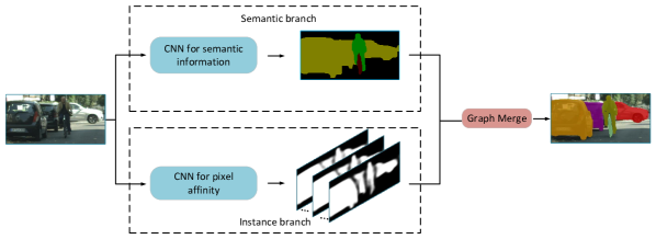
Figure 1: Basic structure for proposed framework.

3 Our Approach

3.1 Overview

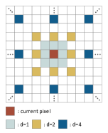
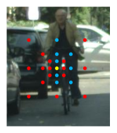
Figure 2: Illustration for pixel affinity. (a) Locations for proposed neighbors. (b) The yellow point indicates the current pixel. Other points are neighboring pixels, in which red ones indicate pixels of different instances and blue ones indicate the same instance (rider). The pixel distance is NOT real but only for an illustration. (c) The derived labels and expected network output.

The fundamental framework of our approach is shown in Fig. 1. We propose to split the task of instance segmentation into two sequential steps. The first step utilizes CNN to obtain class information and pixel affinity of the input image, while the second step applies the graph merge algorithm on those results to generate the pixel-level masks for each instance.

In the first step, we utilize semantic segmentation network to generate the class information for each pixel. Then, we use another network to generate information which is helpful for instance segmentation. It is not straightforward to make the network output pixel-level instance label directly, as labels of instance are exchangeable. Under this circumstance, we propose to learn whether a pair of neighboring pixels belongs to the same instance. It is a binary classification problem that can be handled by the network.

It is impractical to generate affinities between each pixel and all the others in an image. Thus, we carefully select a set of neighboring pixels to generate affinity information. Each channel of the network output represents a probability of whether the neighbor pixel and the current one belong to the same instance, as illustrated in Fig. 2. As can be seen from the instance branch in Fig. 1, the pixel affinities indicate the boundary apparently and show the feasibility to represent the instance information.

In the second step, we consider the whole image as a graph and apply the graph merge algorithm on the network output to generate instance segmentation results. For every instance, the class label is determined by voting among all pixels based on sementic labels.

3.2 Semantic Branch

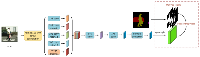
Figure 3: Basic structure for instance branch, we utilize the basic framework from Deeplabv3 [7] based on Resnet-101 [25].

Deeplabv3 [7] is one of the state-of-the-art networks in semantic segmentation. Thus, we use it as semantic branch in our proposed framework. It should be noted that other semantic segmentation approaches could also be used in our framework.

3.3 Instance Branch

We select several pixel pairs, and the output of instance branch represents whether they belong to the same instance. Theoretically, if an instance is composed of only one connected area, we could merge the instance with only two pairs of pixel affinity, i.e. whether $(p(x,y),p(x-1,y))$ and $(p(x,y),p(x,y-1))$ belong to the same instance, $p(x,y)$ is the pixel at location $(x,y)$ in an image $I$. For the robustness to noise and the ability to handle fragmented instances, we choose the following pixel set as the neighborhood of current pixel $p(x,y)$

$$N(x,y)=\bigcup_{d\in D}N_{d}(x,y),$$ (1)

where $N_{d}(x,y)$ is the set of eight-neighbors of $p(x,y)$ with distance $d$, which can be expressed as

$$N_{d}(x,y)=\{p(x+a,y+b),\forall a,b\in\{d,0,-d\}\}\setminus\{p(x,y)\},$$ (2)

and $D$ is the set of distances. In our implementation, $D=\{1,2,4,8,16,32,64\}$, as illustrated in Fig. 2.

We employ the network in Fig. 3 as the instance branch, in which we remove the last softmax activation of semantic segmentation network and minimize the cross entropy loss after sigmoid activation. There are $8\times 7=56$ elements in the set $N(x,y)$, so we assign $56$ channels to the last layer. In the training procedure, the corresponding label is assigned as 1 if the pixel pair belongs to a same instance. In the inference procedure, we treat the network outputs as the probability of the pixel pair belonging to the same instance. We make a simple illustration of the selected neighbors in Fig. 2, and the corresponding label is shown in Fig. 2.

3.4 Graph Merge

Figure 4: A brief illustration for graph merge algorithm

The graph merge algorithm takes the semantic segmentation and pixel affinity results as input to generate instance segmentation results. Let vertex set $V$ be the set of pixels and edge set $E$ be the set of pixel affinities obtained from network. Then, we have a graph $G=(V,E)$. It should be noted that the output of the instance branch is symmetrical. Pair $(p(x,y),p(x_{c},y_{c}))$ obtained at $(x,y)$ and $(p(x_{c},y_{c}),p(x,y))$ at $(x_{c},y_{c})$ have same physical meaning, both indicating the probability of these two pixels belonging to a certain instance. We average the corresponding probabilities before using them as the initial $E$. Thus, $G$ can be considered as an undirected graph.

Let $e(i,j)$ denote an edge connecting vertex $i$ and $j$. We first find the edge $e(u,v)$ with maximum probability and merge $u,v$ together into a new super-pixel $uv$. It should be noted that we do not distinguish pixel and super-pixel explicitly, and $uv$ is just a symbol indicating it is merged from $u$ and $v$. After merging $u,v$, we need to update the graph $G$. For vertex set $V$, two pixels are removed and a new super-pixel is added,

$$V:=V\setminus\{u,v\}\cup\{uv\}.$$ (3)

Then, the edge set $E$ needs to be updated. We define $E(u)=\bigcup_{k\in K_{u}}\{e(u,k)\}$ representing all edges connecting with $u$. $K_{u}$ is the set of pixels connecting to $u$. $E(u)$ and $E(v)$ should be discarded as $u$ and $v$ have been removed. $K_{uv}=K_{u}\cup K_{v}\setminus\{u,v\}$, $E$ is updated as follows,

$$E:=E\setminus E(u)\setminus E(v)\bigcup_{k\in K_{uv}}\{e(uv,k)\}.$$ (4)

For $k\in K(u)\cap K(v)$, $e(uv,k)$ is the average of $e(u,k)$ and $e(v,k)$. Otherwise, $e(uv,k)$ inherits from $e(u,k)$ or $e(v,k)$ directly.

After updating $G$, we continue to find a new maximum edge and repeat the procedure iteratively until the maximum probability is smaller than the threshold $r_{w}$. We summarize the procedure above in Algorithm 1. We then obtain a set of $V$ and each pixel/super-pixel represents an instance. We recover the super-pixels to sets of pixels and filter the sets with a cardinality threshold $r_{c}$ which means we only preserve the instance with pixels more than $r_{c}$. We get a set of pixels $X$ as an instance and calculate the confidence of the instance from the initial $E$. We average all the edges $e(i,j)$ for both $i,j\in X$, and this confidence indicates the probability of $X$ being an instance.

Algorithm 1 Graph Merge Algorithm

0:  Averaged instance branch output $P(u,v)$, thresholds $r_{w}$

0:  Merge result $V$, $E$

1:  Initialize $V$ with pixels and $E$ with $e(u,v)=P(u,v)$

2:  while Maximum $e(u,v)\in E\geq r_{w}$ do

3:     Merge $u,v$ to super-pixel $uv$

4:     Update $V$: $V\Leftarrow V\setminus\{u,v\}\cup\{uv\}$

5:     $K_{uv}=K_{u}\cup K_{v}\setminus\{u,v\}$

6:     for $k\in K_{u,v}$ do

7:        if $k\in E(u)\cap E(v)$ then

8:           $e(uv,k)$ is the average of $e(u,k)$ and $e(v,k)$

9:        else

10:           $e(uv,k)=k\in K_{u}?\ e(u,k):e(v,k)$

11:        end if

12:     end for

13:     Update $E$: $E\Leftarrow E\setminus E(u)\setminus E(v)\bigcup_{k\in K_{uv}}\{e(uv,k)\}$

14:  end while

We prefer the spatially neighboring pixels to be merged together. Thus, we divide $D=\{1,2,4,8,16,32,64\}$ as three subsets $D_{s}=\{1,2,4\},\ D_{m}=\{8,16\}$ and $D_{l}=\{32,64\}$ with which we do our graph merge sequentially. Firstly, we merge pixels with probabilities in $D_{s}$ with a large threshold $r_{ws}=0.97$, and then all edges with distances in $D_{m}$ will be added. We continue our graph merge with a lower threshold $r_{wm}=0.7$ and repeat the operation for $D_{l}$ with $r_{wl}=0.3$.

4 Implementation Details

The fundamental framework of our approach has been introduced in the previous section. In this section, we elaborate the implementation details.

4.1 Excluding Background

Background pixels are not necessary to be considered in the graph merge procedure, since they should not be present in any instance. Excluding them decrease the image size as well as accelerate the whole process. We refer the interested sub-regions containing foreground objects as ROI in our method. Different from the ROI in proposal-based method, the ROI in our method may contain multiple objects. In the implementation, we look for connected areas of foreground pixels as ROIs. The foreground pixels will be aggregated to super-pixels when generating feasible areas for connecting the separated components belonging to a certain instance. In our implementation, the super-pixel is 32x32, which means if any pixel in a 32x32 region is foreground pixel, we consider the whole 32x32 region as foreground. We extend the connected area with a few pixels (16 in our implementation) and find the tightest bounding boxes, which is used as the input of our approach. Different from thousands of proposals used in the proposal-based instance segmentation algorithms, the number of ROIs in our approach is usually less than 10.

4.2 Pixel Affinity Refinement

Besides determining the instance class, the semantic segmentation results can help more with the graph merge algorithm. Intuitively, if two pixels have different semantic labels, they should not belong to a certain instance. Thus, we propose to refine the pixel affinity output from the instance branch in Fig. 1 by scores from the semantic branch. Denote $P(x,y,c)$ as the probability of $p(x,y)$ and $p(x_{c},y_{c})$ belonging to a certain instance from the instance branch, we refine it by multiplying the semantic similarity of these two pixels.

Let $\mathbf{P}(x,y)=(p_{0}(x,y),p_{1}(x,y),\cdots,p_{m}(x,y))$ denote the probability output of the semantic branch. $m+1$ denotes the number of the classes (including background), $p_{i}(x,y)$ denotes the probability of the pixel belonging to the $i$-th class and $p_{0}(x,y)$ is background probability. The inner product of the probabilities of two pixels indicates the probability of these two pixels having a certain semantic label. We do not care background pixels, so we discard the background probability and calculate the inner product of $\mathbf{P}(x,y)$ and $\mathbf{P}(x_{c},y_{c})$ as $\sum_{i=1}^{m}p_{i}(x,y)p_{i}(x_{c},y_{c})$. We then refine the pixel affinity by

$$P_{r}(x,y,c)=\sigma(\sum_{i=1}^{m}p_{i}(x,y)p_{i}(x_{c},y_{c}))P(x,y,c),$$ (5)

where

$$\sigma(x)=2\times(\frac{1}{1+e^{-\alpha x}}-\frac{1}{2}).$$ (6)

This $\sigma()$ function is modified from sigmoid function and we set $\alpha=5$ to weaken the influence of the semantic inner product.

Despite the information we mentioned above, we find that the semantic segmentation model may confuse among classes. Thus, we define the confusion matrix. Confusion matrix in semantic segmentation means a matrix where $c_{ij}$ represents the count of pixels belonging to class $i$ classified to class $j$. Given this, we can find that the semantic segmentation model sometimes misclassifies a pixel in a subclass, but rarely across sets. Thus, we combine classes in each set together as a super-class to further weaken the influence on instance segmentation from the semantic term. Moreover, we set the inner product to 0, when the two pixels are in different super-classes, which helps to refine the instance segmentation result.

4.3 Resizing ROIs

Like what ROI pooling does, we enlarge the shorten edge of the proposed boxes to a fixed size and proportionally enlarge the other edge, with which we use as the input. For the Cityscapes dataset, we scale the height of each ROI to 513, if the original height is smaller than it. The reason of scaling it to 513 is that the networks are trained with 513x513 patches. Thus, we would like to use the same value for inference. Moreover, we limit the scaling factor to be less than 4. Resizing ROIs is helpful to find more small instances.

4.4 Forcing Local Merge

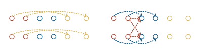
Figure 5: Illustration for forcing local merge. We simulate the merging process with distance $\{1,2,4\}$ and window size 2, we only show edges involved in this process. Pixels with identical color are to be merged and we need to update the new weights for edges. Left graph shows that the new probability in distance $\{2\}$ should only be averaged by original weights from distance $\{4\}$ in the same direction. However, the right graph shows the new probability for distance $\{1\}$ should be an average for edges from both distance $\{1\}$ and $\{2\}$.

We force the neighboring $m\times m$ pixels to be merged before the graph merge. During the process, we recalculated the pixel affinities according to our graph algorithm in Sec. 3.4. Fig. 5 shows a simple example. Force merging neighboring pixels can not only filter out the noises of the network output by averaging, but also decrease the input size of the graph merge algorithm to save processing time. We will provide results on different merge window size in Sec 5.3.

4.5 Semantic Class Partition

To get more exquisite ROIs, we refer to the semantic super-classes in Sec. 4.2 and apply it on the procedure of generating connected areas. We sum the probabilities in each super-class and classify the pixels to super-classes. To find foreground region of a super-class, we only consider the pixels classified to this super-class as foreground and all the others as background. Detailed experimental results will be provided in Sec. 5.3

5 Experimental Evaluation

We evaluate our method on the Cityscapes dataset [9], which consists of $5,000$ images representing complex urban street scenes with the resolution of $2048\times 1024$. Images in the dataset are split into training, validation, and test set of $2,975$, $500$, and $1,525$ images, respectively. We use average precision (AP) as our metric to evaluate the results, which is calculated by the mean of IOU threshold from 0.5 to 0.95 with the step of 0.05.

As most of the images in Cityscapes dataset are background on top or bottom, we discard the parts with no semantic labeled pixels on top or bottom for 90% of training images randomly, in order to make our data more effective. To improve the performance of semantic segmentation, we utilize coarse labeled training data by selecting patches containing trunk, train and bus as additional training data to train the semantic branch. We crop 1554 patches from coarse labeled data. To augment data with different scale objects, we also crop several upsampled areas in the fine labeled data. As a result, the final patched fine labeled training data includes 14178 patches, including 2975 original training images with 90% of them dropped top and bottom background pixels. The networks are trained with Tensorflow [1] and the graph merge algorithm is implemented in C++.

5.1 Training Strategy

For the basic setting, the network output strides for both semantic and instance branch are set to 16, and they are trained with input images of size $513\times 513$.

For the semantic branch, the network structure is defined as introduced in Sec. 3.2, whose weight is initialized with ImageNet [45] pretrained ResNet-101 model. During training, we use 4 Nvidia P40 GPUs with SGD [31] in the following steps. (1) We use 19-class semantic labeled data in Cityscapes dataset fine and coarse data together, with initial learning rate of 0.02 and batch size of 16 per GPU. Model is trained using 100k iterations and learning rate is multiplied by 0.7 every 15k iterations. (2) As the instance segmentation only focuses on 8 foreground objects, we then finetune the network with 9 classes labeled data (8 foreground objects and 1 background). Training data for this model contains a mix of 2 times fine labeled patched data and coarse labeled patches. We keep the other training setting unchanged. (3) We finetune the model with 3 times of original fine labeled data together with coarse labeled patches, with other training setting unchanged.

For the instance branch, we still initialize the network parameter with ImageNet pretrained models. We train this model with patched fine labeled training data for 120k iterations, with other settings identical to the step (1) for semantic model training.

5.2 Main Results

As shown in Table 1, our method notably improves the performance and achieves 27.3 AP on Cityscapes test set, which outperforms Mask RCNN trained with only Cityscapes train data by 1.1 points (4.2% relatively).

We show qualitive results for our algorithm in Fig. 6. As shown in the figure, we produce high quality results on both semantic and instance masks, where we get precise boundaries. As shown in the last row of result, we can handle the problem of fragmented instances and merge the separated parts together.

Our method outperforms Mask RCNN on AP but gets a relatively lower performance on AP 50%. We would interpret it as we could get higher score when the IOU threshold is larger. It means that Mask RCNN could find more instances with relatively less accurate masks (higher AP 50%), but our method could obtain more accurate boundaries. The bounding box of proposal-based method may lead to a rough mask, which will be judged as correct with small IOU.

Utilizing the implementation of Mask RCNN in Detectron, we generate the instance masks and compare them with our results. As shown in Fig. 7, our results are finer grained. It can be expected that results will be better if we substitute the mask from Mask RCNN with ours when both approaches have prediction of a certain instance.

Table 1: Instance segmentation performance on test set of Cityscapes, all results listed are trained with only Cityscapes dataset

Methods	person	rider	car	trunk	bus	train	mcycle	bicycle	AP 50%	AP
InstanceCut[29]	10.0	8.0	23.7	14.0	19.5	15.2	9.3	4.7	27.9	13.0
SAIS[22]	14.6	12.9	35.7	16.0	23.2	19.0	10.3	7.8	36.7	17.4
DWT[3]	15.5	14.1	31.5	22.5	27.0	22.9	13.9	8.0	35.3	19.4
DIN[2]	16.5	16.7	25.7	20.6	30.0	23.4	17.1	10.1	38.8	20.0
SGN[37]	21.8	20.1	39.4	24.8	33.2	30.8	17.7	12.4	44.9	25.0
Mask RCNN[23]	30.5	23.7	46.9	22.8	32.2	18.6	19.1	16.0	49.9	26.2
Ours	31.5	25.2	42.3	21.8	37.2	28.9	18.8	12.8	45.6	27.3

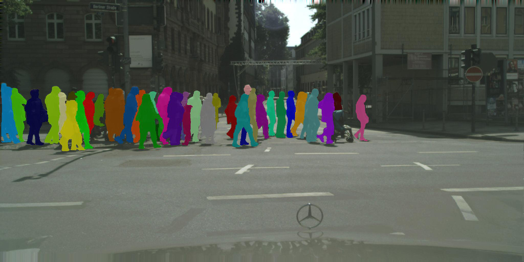
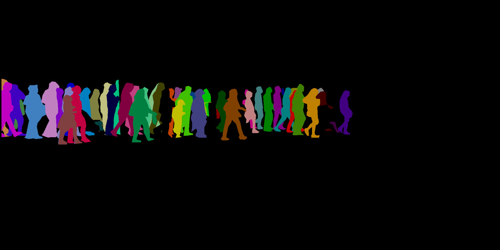
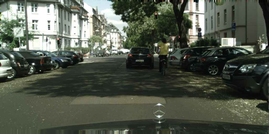
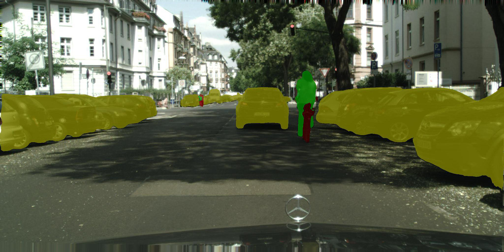
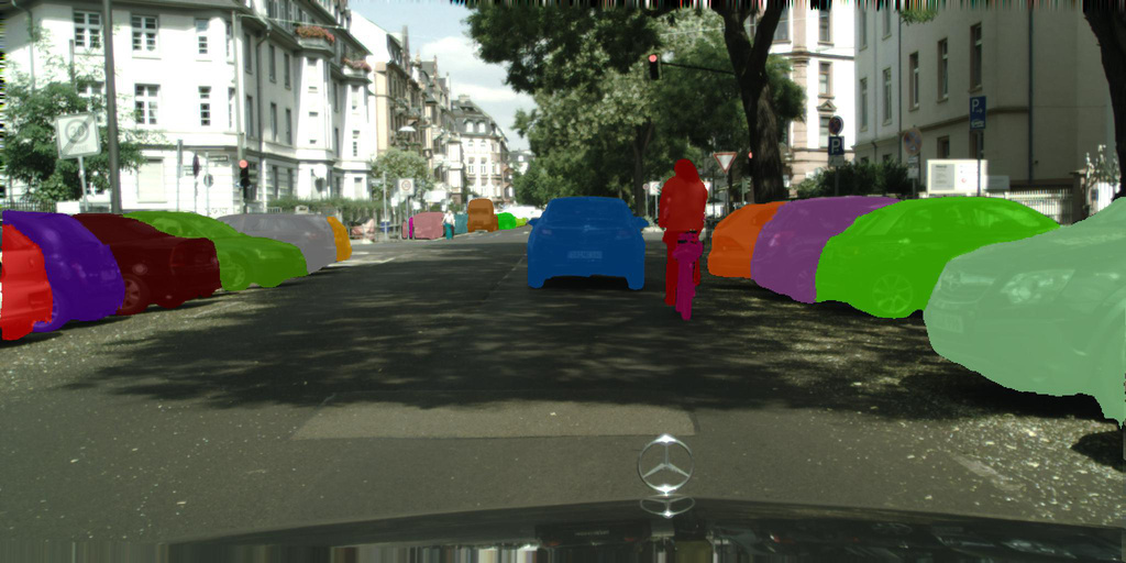
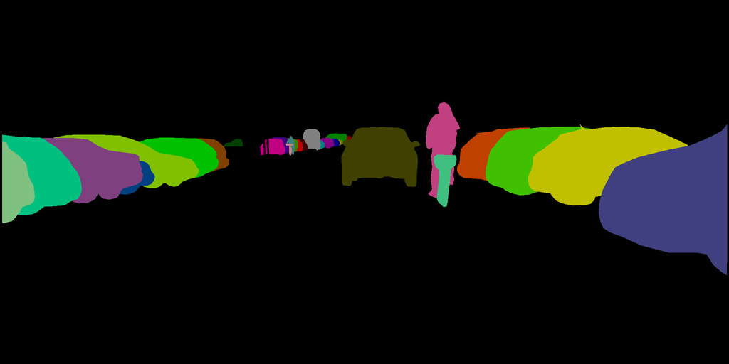
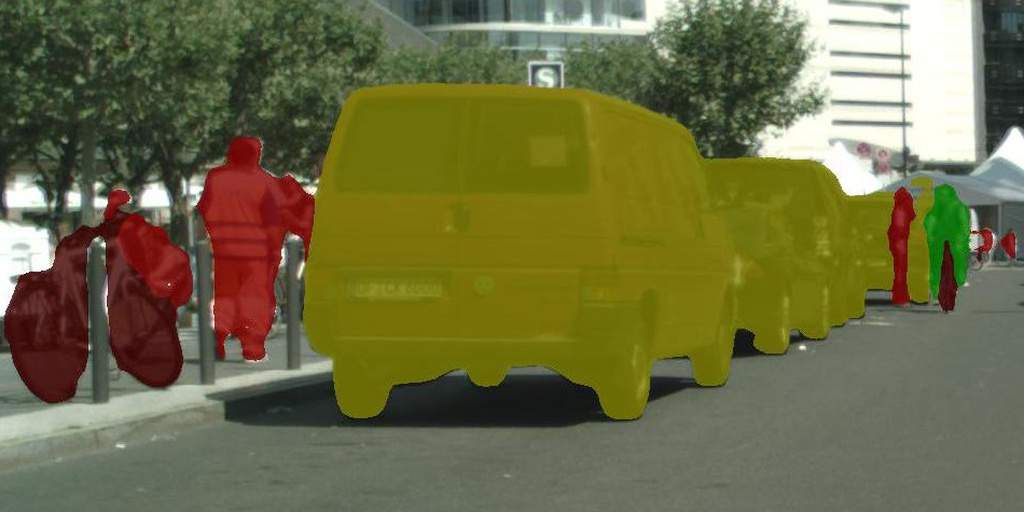
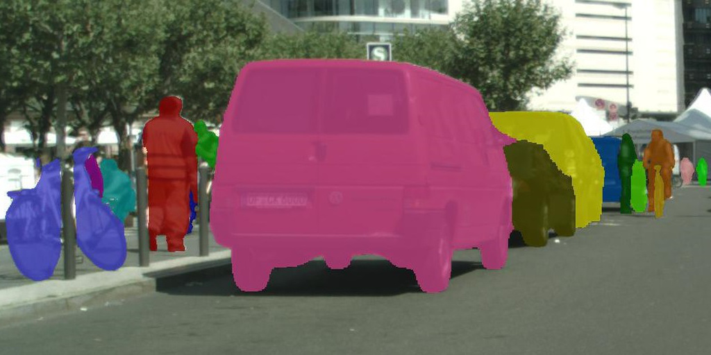
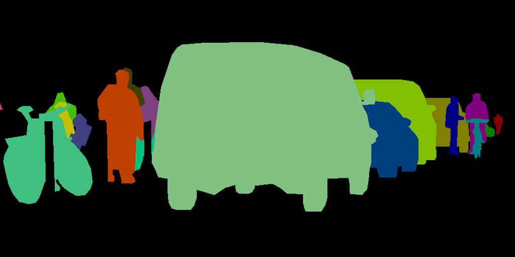
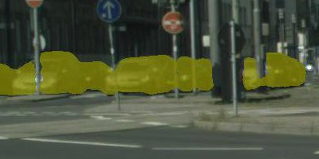
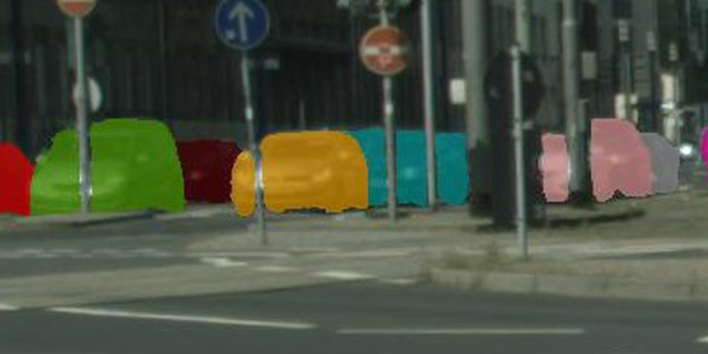
Figure 6: Results on Cityscapes val dataset, original image, semantic result, instance result and ground truth from left to right. Results in last two rows are cropped from original ones for better visualization.

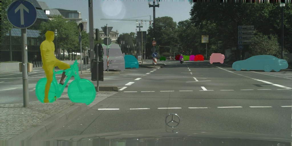
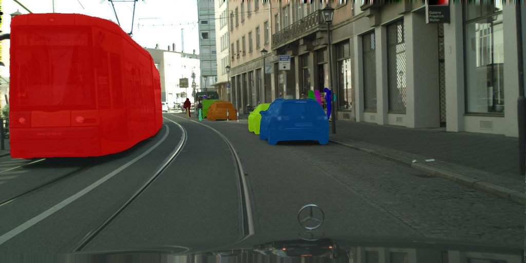
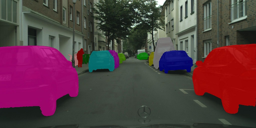
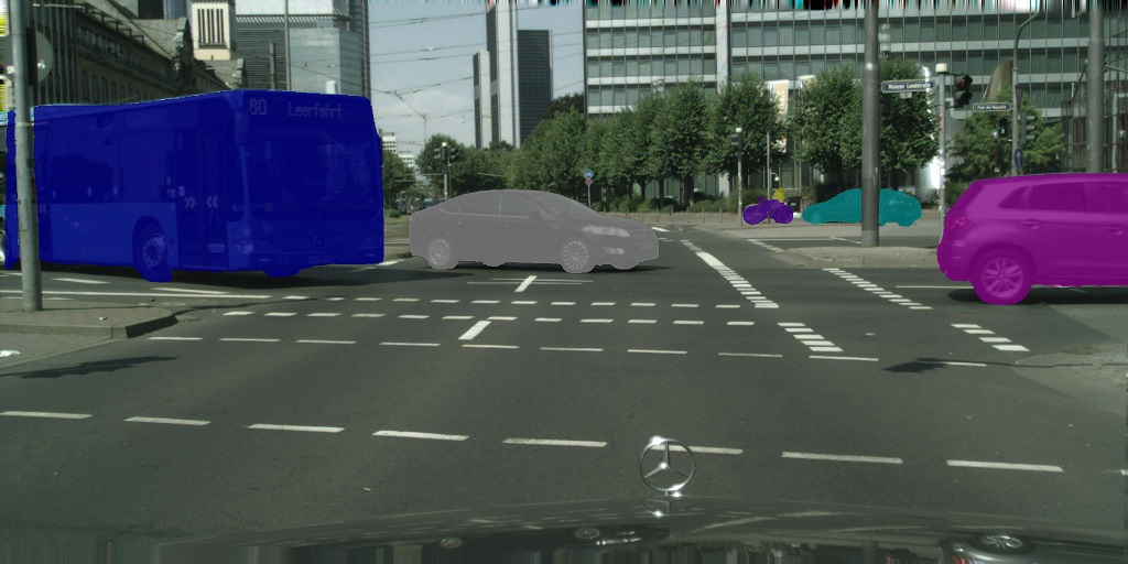
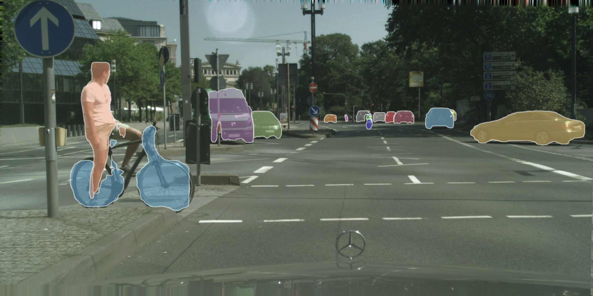
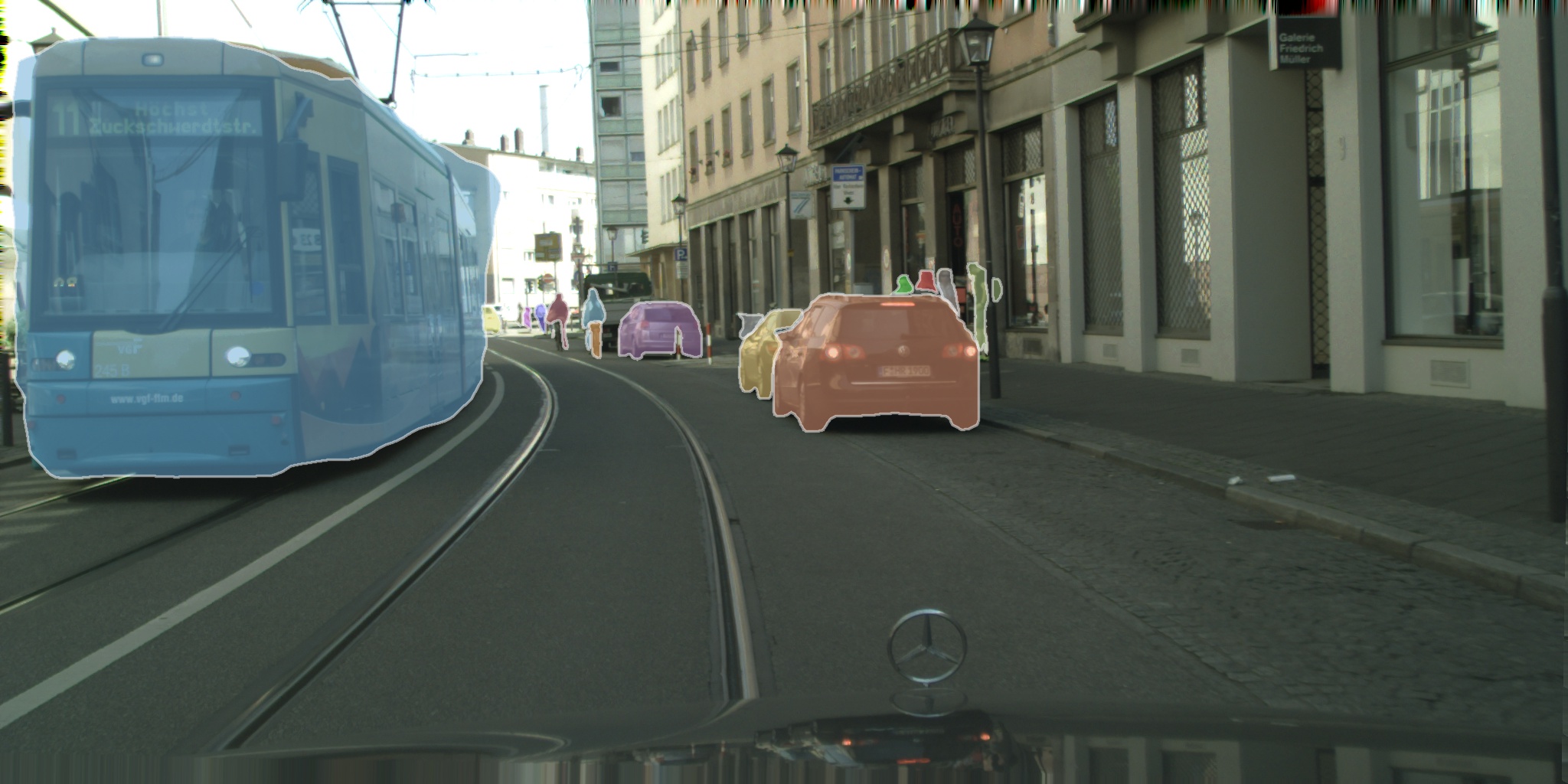
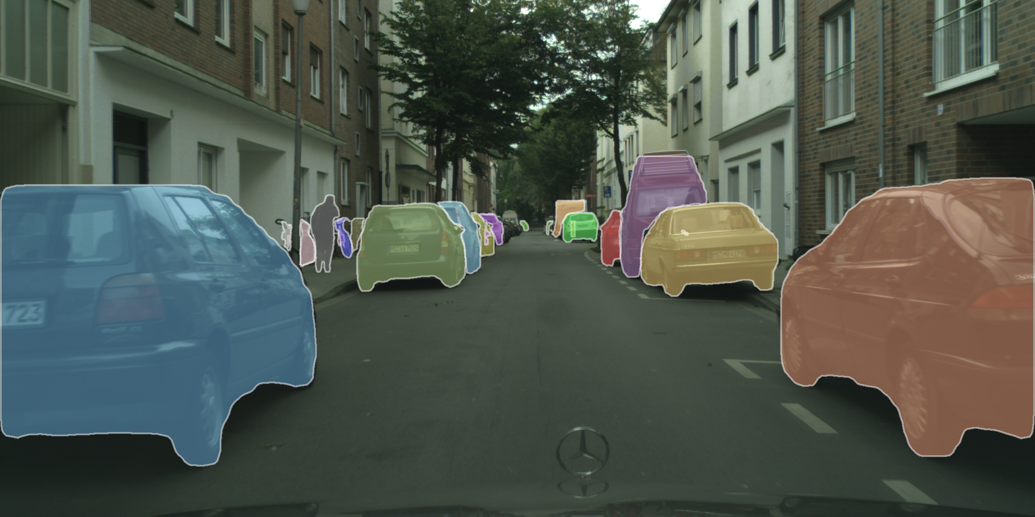
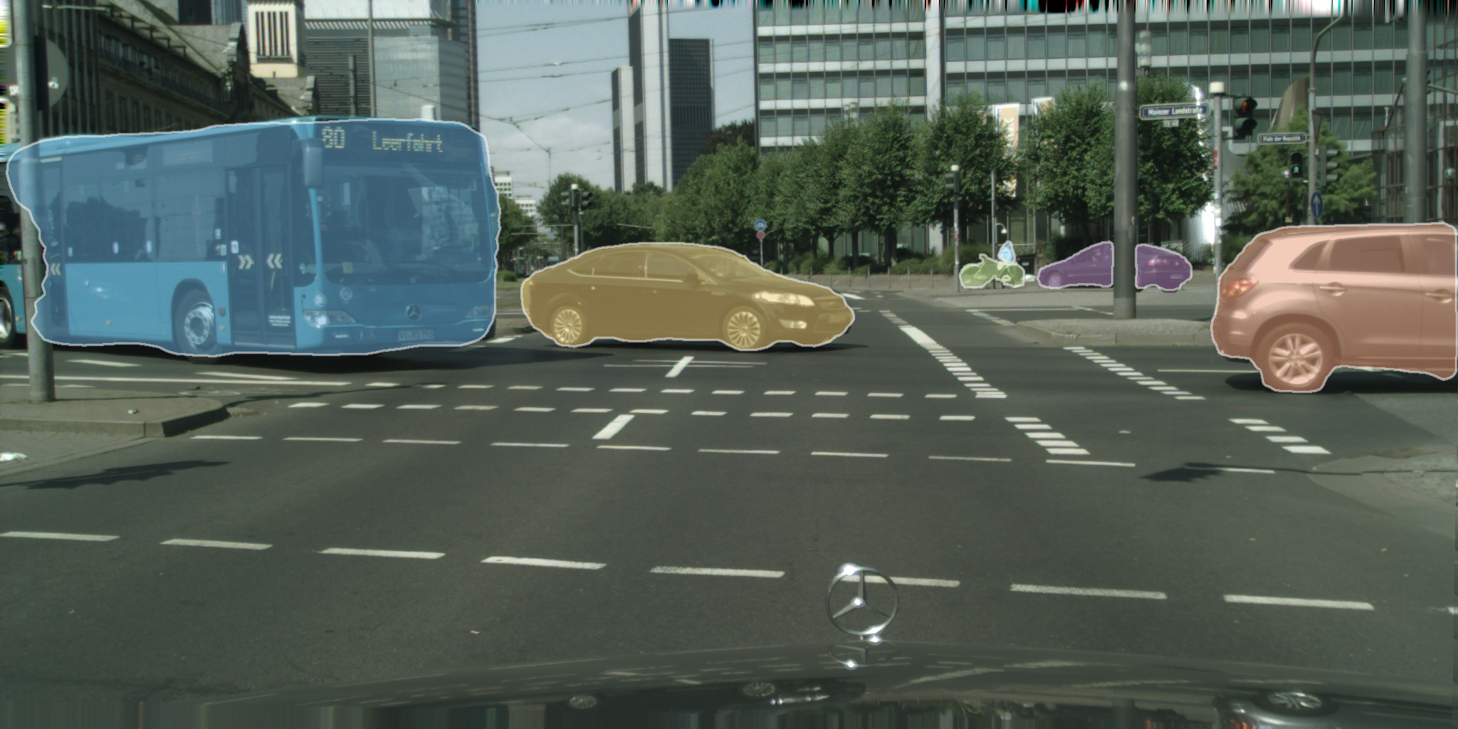
Figure 7: Results compared with Mask RCNN. The first row are our results and the second row are results from Mask RCNN. As shown in the figure, we generate more fine-grained masks.

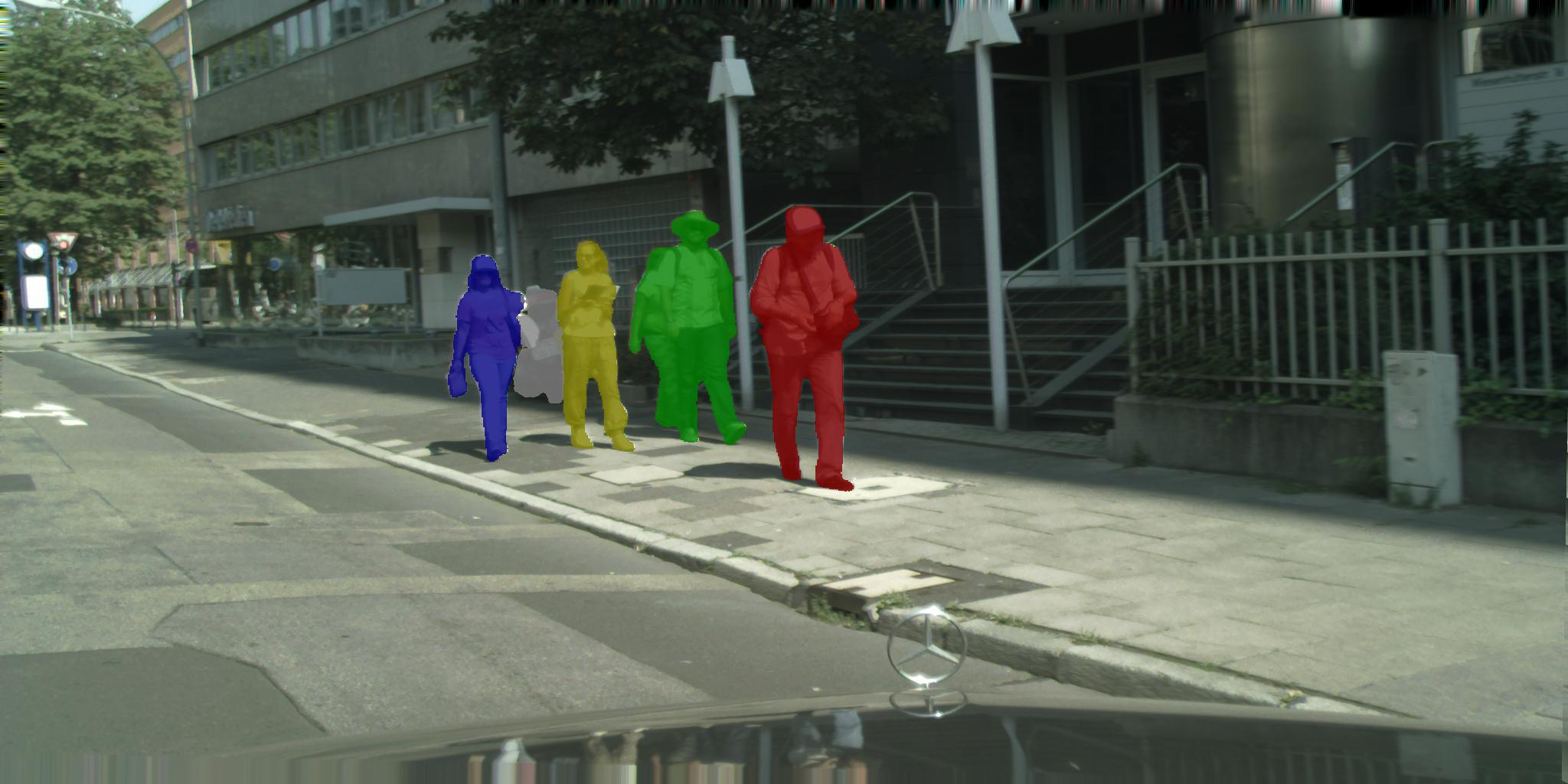
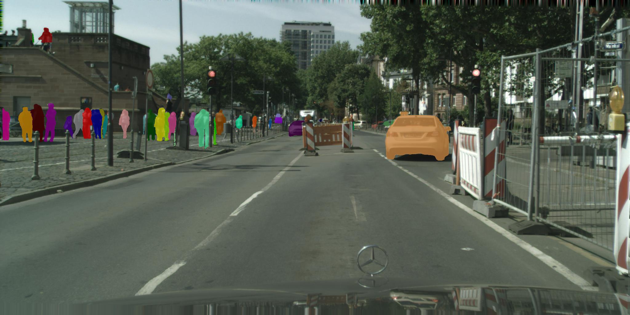
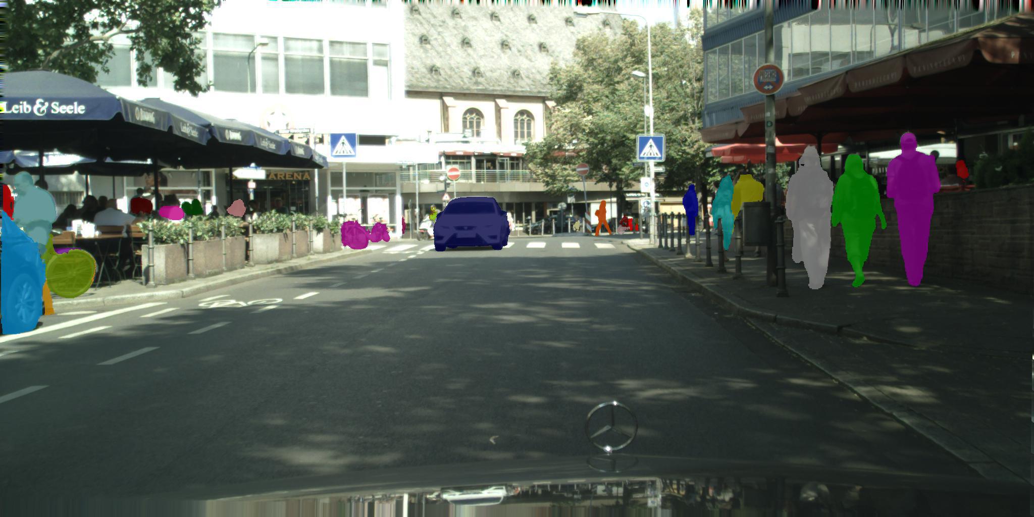
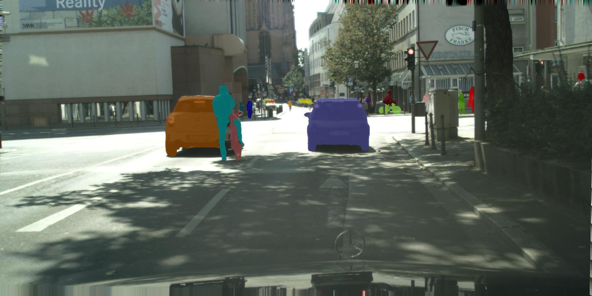
Figure 8: Examples of faliure case

5.3 Detailed Results

We report the ablation studies with val set and discuss in detail.

Baseline: we take the algorithm we describe before Sec. 4.1 as the baseline, for excluding backgrounds helps to significantly speedup the graph merge algorithm and hardly affects the final results. We get 18.9% AP as our baseline, and we will introduce the results for strategies applied to graph merge algorithm.

Table 2: Graph Merge Strategy: we test for our graph merge strategies for our algorithm including PAR: Pixel Affinity Refinement, RR: Resizing ROIs, FLM: Forcing Local Merge and SCP: Semantic Class Partition. Note that 2 and 4 in FLM represent the merge window size, default as 1.

PAR	RR	FLM	SCP	AP
				18.9
✓				22.8
✓	✓			28.7
✓	✓	2		29.2
✓	✓	4		27.5
✓	✓	2	✓	30.7

We show the experimental results for graph merge strategies in Table. 2. For pixel affinity refinement, we add semantic information to refine the probability and get a 22.8% AP result. As shown in the table, it provides 3.9 points AP improvement. Then we resize the ROIs with a fix size 513, and we get a raise of 5.9 points AP, which significantly improve the result. Merge window size influences the result a lot. We have a 0.5 point improvement utilizing window size 2 and a 1.2 point drop with window size 4. As we can see, utilizing 2 as the window size not only reduce the complexity of graph merge, but also get improvement on performance, but utilizing 4 will cause a lost on detailed information and perform below expectation. Therefore, we utilize 2 in the following experiments. As mentioned in Sec. 4.1, we finally divided semantic classes into 3 subclasses for semantic class partition:{person, rider}, {car, trunk, bus, train} and {motorcycle, bicycle}, finding feasible areas separately. Such separation reduces the influence across subclasses and makes the ROI resize more effective. We get a 1.5 improvement by applying this technique from 29.0% to 30.5%, as shown in the table. It is noted that utilizing larger image can make results better, but it also increases the processing time.

Besides the strategies we utilize in the graph merge, we also test our model for different inference strategies referring to [7]. Output stride is always important for the segmentation-like task. Small output stride usually means more detailed information but more inference time cost and smaller batch size in training. We test our models firstly trained on output stride 16, then we finetuned models on output stride 8 as in [7]. It shows in Table. 3 that both semantic and instance model finetuned with output stride 8 improve the result by 0.5 point individually. When combined together, we achieve 32.1% AP with 1.4 point improvement compared with output stride 16.

We apply horizontal flips and semantic class refinement as alternative inference strategies. Horizontal flips for semantic inference brings 0.7 point increase in AP, and for instance inference flip, 0.5 point improvement is observed. We then achieve 33.5% AP combining these two flips.

Table 3: Additional inference strategies: We test for additional inference strategies for our algorithm including Semantic OS: output stride for semantic branch, Instance OS: output stride for instance branch SHF: Semantic horizontal flip inference,IHF: Instance horizontal flip inference and SCR: Semantic Class Refinement. We also list several results from other methods for comparison.

Methods	Semantic OS	Instance OS	SHF	IHF	SCR	AP
DWT[3]						21.2
SGN[37]						29.2
Mask RCNN[23]						31.5
Ours	16	16				30.7
	8	16				31.2
	16	8				31.2
	8	8				32.1
	8	8	✓			32.8
	8	8		✓		32.6
	8	8	✓	✓		33.5
	8	8	✓	✓	✓	34.1

Through observations on the val set, we find that instances in bicycle and motorcycle often fail to be connected when they are fragmentated. To improve such situation, we map the pixel affinities between these two classes with Equ. 6 at the last distance $d=64$. As shown in Table 3, semantic class refinement get 0.6 point improvement, and get our best result 34.1% AP on the val set.

5.4 Discussions

In our current implementation, the maximum distance of the instance branch output is 64. It means that the graph merge algorithm is not able to merge two non-adjacent parts if the distance is greater than 64. Adding more output channels can hardly help the overall performance. Moreover, using other network structures, which could achieve better results on the semantic segmentation, may further improve the performance of the proposed graph merge algorithm. Some existing methods, such as [32], could solve the graph merge problem but [32] is much slower than the proposed method. The current graph merge step is implemented on CPU and we believe there is big potential to use multi-core CPU system for acceleration. Some examples of failure case are shown in Fig. 8. The proposed method may miss some small objects or merge different instances together by mistake.

6 Conclusions

In this paper, we introduce a proposal-free instance segmentation scheme via affinity derivation and graph merge. We generate semantic segmentation results and pixel affinities from two separate networks with a similar structure. Taking these information as input, we regard pixels as vertexes and pixel affinity information as edges to build a graph. The proposed graph merge algorithm is then used to cluster the pixels into instances. Our method outperforms Mask RCNN on Cityscapes dataset by 1.1 point AP improvement using only Cityscapes training data. It shows that proposal-free method can achieve state-of-the-art performance. We notice that the performance of semantic segmentation keep improvement with new methods, which can easily lead to performance improvement for instance segmentation via our method. The proposed graph merge algorithm is simple. We believe that more advanced algorithms can lead to even better performance. Improvements along these directions are left for further work.

- [1] Abadi, M., Agarwal, A., Barham, P., Brevdo, E., Chen, Z., Citro, C., Corrado, G.S., Davis, A., Dean, J., Devin, M., et al.: Tensorflow: Large-scale machine learning on heterogeneous distributed systems. arXiv preprint arXiv:1603.04467 (2016)
- [2] Arnab, A., Torr, P.H.S.: Pixelwise instance segmentation with a dynamically instantiated network. In: 2017 IEEE Conference on Computer Vision and Pattern Recognition (CVPR). pp. 879–888 (July 2017). https://doi.org/10.1109/CVPR.2017.100
- [3] Bai, M., Urtasun, R.: Deep watershed transform for instance segmentation. In: 2017 IEEE Conference on Computer Vision and Pattern Recognition (CVPR). pp. 2858–2866 (July 2017). https://doi.org/10.1109/CVPR.2017.305
- [4] Brabandere, B.D., Neven, D., Gool, L.V.: Semantic instance segmentation for autonomous driving. In: 2017 IEEE Conference on Computer Vision and Pattern Recognition Workshops (CVPRW). pp. 478–480 (July 2017). https://doi.org/10.1109/CVPRW.2017.66
- [5] Chen, L.C., Papandreou, G., Kokkinos, I., Murphy, K., Yuille, A.L.: Deeplab: Semantic image segmentation with deep convolutional nets, atrous convolution, and fully connected crfs. IEEE Transactions on Pattern Analysis and Machine Intelligence 40(4), 834–848 (April 2018). https://doi.org/10.1109/TPAMI.2017.2699184
- [6] Chen, L.C., Hermans, A., Papandreou, G., Schroff, F., Wang, P., Adam, H.: Masklab: Instance segmentation by refining object detection with semantic and direction features. arXiv preprint arXiv:1712.04837 (2017)
- [7] Chen, L.C., Papandreou, G., Schroff, F., Adam, H.: Rethinking atrous convolution for semantic image segmentation. arXiv preprint arXiv:1706.05587 (2017)
- [8] Chen, L.C., Zhu, Y., Papandreou, G., Schroff, F., Adam, H.: Encoder-decoder with atrous separable convolution for semantic image segmentation. arXiv preprint arXiv:1802.02611 (2018)
- [9] Cordts, M., Omran, M., Ramos, S., Rehfeld, T., Enzweiler, M., Benenson, R., Franke, U., Roth, S., Schiele, B.: The cityscapes dataset for semantic urban scene understanding. In: 2016 IEEE Conference on Computer Vision and Pattern Recognition (CVPR). pp. 3213–3223 (June 2016). https://doi.org/10.1109/CVPR.2016.350
- [10] Dai, J., He, K., Sun, J.: Instance-aware semantic segmentation via multi-task network cascades. In: 2016 IEEE Conference on Computer Vision and Pattern Recognition (CVPR). pp. 3150–3158 (June 2016). https://doi.org/10.1109/CVPR.2016.343
- [11] Dai, J., Qi, H., Xiong, Y., Li, Y., Zhang, G., Hu, H., Wei, Y.: Deformable convolutional networks. In: 2017 IEEE International Conference on Computer Vision (ICCV). pp. 764–773 (Oct 2017). https://doi.org/10.1109/ICCV.2017.89
- [12] Dai, J., He, K., Li, Y., Ren, S., Sun, J.: Instance-sensitive fully convolutional networks. In: Leibe, B., Matas, J., Sebe, N., Welling, M. (eds.) Computer Vision – ECCV 2016. pp. 534–549. Springer International Publishing, Cham (2016)
- [13] Dai, J., Li, Y., He, K., Sun, J.: R-fcn: Object detection via region-based fully convolutional networks. In: Advances in neural information processing systems. pp. 379–387 (2016)
- [14] Erhan, D., Szegedy, C., Toshev, A., Anguelov, D.: Scalable object detection using deep neural networks. In: 2014 IEEE Conference on Computer Vision and Pattern Recognition. pp. 2155–2162 (June 2014). https://doi.org/10.1109/CVPR.2014.276
- [15] Fathi, A., Wojna, Z., Rathod, V., Wang, P., Song, H.O., Guadarrama, S., Murphy, K.P.: Semantic instance segmentation via deep metric learning. arXiv preprint arXiv:1703.10277 (2017)
- [16] Fu, J., Liu, J., Wang, Y., Lu, H.: Stacked deconvolutional network for semantic segmentation. arXiv preprint arXiv:1708.04943 (2017)
- [17] Garcia-Garcia, A., Orts-Escolano, S., Oprea, S., Villena-Martinez, V., Garcia-Rodriguez, J.: A review on deep learning techniques applied to semantic segmentation. arXiv preprint arXiv:1704.06857 (2017)
- [18] Girshick, R.: Fast r-cnn. In: 2015 IEEE International Conference on Computer Vision (ICCV). pp. 1440–1448 (Dec 2015). https://doi.org/10.1109/ICCV.2015.169
- [19] Girshick, R., Donahue, J., Darrell, T., Malik, J.: Rich feature hierarchies for accurate object detection and semantic segmentation. In: 2014 IEEE Conference on Computer Vision and Pattern Recognition. pp. 580–587 (June 2014). https://doi.org/10.1109/CVPR.2014.81
- [20] Grauman, K., Darrell, T.: The pyramid match kernel: discriminative classification with sets of image features. In: Tenth IEEE International Conference on Computer Vision (ICCV’05) Volume 1. vol. 2, pp. 1458–1465 Vol. 2 (Oct 2005). https://doi.org/10.1109/ICCV.2005.239
- [21] Hariharan, B., Arbeláez, P., Girshick, R., Malik, J.: Simultaneous detection and segmentation. In: Fleet, D., Pajdla, T., Schiele, B., Tuytelaars, T. (eds.) Computer Vision – ECCV 2014. pp. 297–312. Springer International Publishing, Cham (2014)
- [22] Hayder, Z., He, X., Salzmann, M.: Shape-aware instance segmentation. arXiv preprint arXiv:1612.03129 (2016)
- [23] He, K., Gkioxari, G., Dollár, P., Girshick, R.: Mask r-cnn. In: 2017 IEEE International Conference on Computer Vision (ICCV). pp. 2980–2988 (Oct 2017). https://doi.org/10.1109/ICCV.2017.322
- [24] He, K., Zhang, X., Ren, S., Sun, J.: Delving deep into rectifiers: Surpassing human-level performance on imagenet classification. In: 2015 IEEE International Conference on Computer Vision (ICCV). pp. 1026–1034 (Dec 2015). https://doi.org/10.1109/ICCV.2015.123
- [25] He, K., Zhang, X., Ren, S., Sun, J.: Deep residual learning for image recognition. In: 2016 IEEE Conference on Computer Vision and Pattern Recognition (CVPR). pp. 770–778 (June 2016). https://doi.org/10.1109/CVPR.2016.90
- [26] Huang, J., Rathod, V., Sun, C., Zhu, M., Korattikara, A., Fathi, A., Fischer, I., Wojna, Z., Song, Y., Guadarrama, S., Murphy, K.: Speed/accuracy trade-offs for modern convolutional object detectors. In: 2017 IEEE Conference on Computer Vision and Pattern Recognition (CVPR). pp. 3296–3297 (July 2017). https://doi.org/10.1109/CVPR.2017.351
- [27] Islam, M.A., Rochan, M., Bruce, N.D.B., Wang, Y.: Gated feedback refinement network for dense image labeling. In: 2017 IEEE Conference on Computer Vision and Pattern Recognition (CVPR). pp. 4877–4885 (July 2017). https://doi.org/10.1109/CVPR.2017.518
- [28] Jin, L., Chen, Z., Tu, Z.: Object detection free instance segmentation with labeling transformations. arXiv preprint arXiv:1611.08991 (2016)
- [29] Kirillov, A., Levinkov, E., Andres, B., Savchynskyy, B., Rother, C.: Instancecut: From edges to instances with multicut. In: 2017 IEEE Conference on Computer Vision and Pattern Recognition (CVPR). pp. 7322–7331 (July 2017). https://doi.org/10.1109/CVPR.2017.774
- [30] Lazebnik, S., Schmid, C., Ponce, J.: Beyond bags of features: Spatial pyramid matching for recognizing natural scene categories. In: 2006 IEEE Computer Society Conference on Computer Vision and Pattern Recognition (CVPR’06). vol. 2, pp. 2169–2178 (2006). https://doi.org/10.1109/CVPR.2006.68
- [31] LeCun, Y., Boser, B., Denker, J.S., Henderson, D., Howard, R.E., Hubbard, W., Jackel, L.D.: Backpropagation applied to handwritten zip code recognition. Neural Computation 1(4), 541–551 (Dec 1989). https://doi.org/10.1162/neco.1989.1.4.541
- [32] Levinkov, E., Uhrig, J., Tang, S., Omran, M., Insafutdinov, E., Kirillov, A., Rother, C., Brox, T., Schiele, B., Andres, B.: Joint graph decomposition & node labeling: Problem, algorithms, applications. In: IEEE Conference on Computer Vision and Pattern Recognition (CVPR) (2017)
- [33] Li, Y., Qi, H., Dai, J., Ji, X., Wei, Y.: Fully convolutional instance-aware semantic segmentation. In: 2017 IEEE Conference on Computer Vision and Pattern Recognition (CVPR). pp. 4438–4446 (July 2017). https://doi.org/10.1109/CVPR.2017.472
- [34] Liang, X., Wei, Y., Shen, X., Yang, J., Lin, L., Yan, S.: Proposal-free network for instance-level object segmentation. arXiv preprint arXiv:1509.02636 (2015)
- [35] Lin, G., Shen, C., v. d. Hengel, A., Reid, I.: Efficient piecewise training of deep structured models for semantic segmentation. In: 2016 IEEE Conference on Computer Vision and Pattern Recognition (CVPR). pp. 3194–3203 (June 2016). https://doi.org/10.1109/CVPR.2016.348
- [36] Lin, T.Y., Dollár, P., Girshick, R., He, K., Hariharan, B., Belongie, S.: Feature pyramid networks for object detection. In: 2017 IEEE Conference on Computer Vision and Pattern Recognition (CVPR). pp. 936–944 (July 2017). https://doi.org/10.1109/CVPR.2017.106
- [37] Liu, S., Jia, J., Fidler, S., Urtasun, R.: Sgn: Sequential grouping networks for instance segmentation. In: 2017 IEEE International Conference on Computer Vision (ICCV). pp. 3516–3524 (Oct 2017). https://doi.org/10.1109/ICCV.2017.378
- [38] Liu, W., Anguelov, D., Erhan, D., Szegedy, C., Reed, S., Fu, C.Y., Berg, A.C.: Ssd: Single shot multibox detector. In: Leibe, B., Matas, J., Sebe, N., Welling, M. (eds.) Computer Vision – ECCV 2016. pp. 21–37. Springer International Publishing, Cham (2016)
- [39] Liu, W., Rabinovich, A., Berg, A.C.: Parsenet: Looking wider to see better. arXiv preprint arXiv:1506.04579 (2015)
- [40] Liu, Z., Li, X., Luo, P., Loy, C.C., Tang, X.: Semantic image segmentation via deep parsing network. In: 2015 IEEE International Conference on Computer Vision (ICCV). pp. 1377–1385 (Dec 2015). https://doi.org/10.1109/ICCV.2015.162
- [41] Newell, A., Yang, K., Deng, J.: Stacked hourglass networks for human pose estimation. In: Leibe, B., Matas, J., Sebe, N., Welling, M. (eds.) Computer Vision – ECCV 2016. pp. 483–499. Springer International Publishing, Cham (2016)
- [42] Pinheiro, P.O., Collobert, R., Dollár, P.: Learning to segment object candidates. In: Advances in Neural Information Processing Systems. pp. 1990–1998 (2015)
- [43] Redmon, J., Divvala, S., Girshick, R., Farhadi, A.: You only look once: Unified, real-time object detection. In: 2016 IEEE Conference on Computer Vision and Pattern Recognition (CVPR). pp. 779–788 (June 2016). https://doi.org/10.1109/CVPR.2016.91
- [44] Ren, S., He, K., Girshick, R., Sun, J.: Faster r-cnn: Towards real-time object detection with region proposal networks. IEEE Transactions on Pattern Analysis and Machine Intelligence 39(6), 1137–1149 (June 2017). https://doi.org/10.1109/TPAMI.2016.2577031
- [45] Russakovsky, O., Deng, J., Su, H., Krause, J., Satheesh, S., Ma, S., Huang, Z., Karpathy, A., Khosla, A., Bernstein, M., Berg, A.C., Fei-Fei, L.: Imagenet large scale visual recognition challenge. International Journal of Computer Vision 115(3), 211–252 (Dec 2015). https://doi.org/10.1007/s11263-015-0816-y, https://doi.org/10.1007/s11263-015-0816-y
- [46] Shelhamer, E., Long, J., Darrell, T.: Fully convolutional networks for semantic segmentation. IEEE Transactions on Pattern Analysis and Machine Intelligence 39(4), 640–651 (April 2017). https://doi.org/10.1109/TPAMI.2016.2572683
- [47] Yu, F., Koltun, V.: Multi-scale context aggregation by dilated convolutions. arXiv preprint arXiv:1511.07122 (2015)
- [48] Zhao, H., Shi, J., Qi, X., Wang, X., Jia, J.: Pyramid scene parsing network. In: 2017 IEEE Conference on Computer Vision and Pattern Recognition (CVPR). pp. 6230–6239 (July 2017). https://doi.org/10.1109/CVPR.2017.660