A note on coverings of virtual knots

Abstract.

For a virtual knot $K$ and an integer $r\geq 0$, the $r$-covering $K^{(r)}$ is defined by using the indices of chords on a Gauss diagram of $K$. In this paper, we prove that for any finite set of virtual knots $J_{0},J_{2},J_{3},\dots,J_{m}$, there is a virtual knot $K$ such that $K^{(r)}=J_{r}$ $(r=0\mbox{ and }2\leq r\leq m)$, $K^{(1)}=K$, and otherwise $K^{(r)}=J_{0}$.

1. Introduction

Odd crossings are first introduced for constructing a simple invariant called the odd writhe of a virtual knot by Kauffman [8]. By using odd crossings, Manturov defines a map from the set of virtual knots to itself by replacing the odd crossings with virtual crossings [10].

Later the notion of index is introduced in [2, 4, 6, 11] which assigns an integer to each real crossing such that the parity of the index coincides with the original parity. The $n$-writhe is defined as a refinement of the odd writhe. Jeong defines an invariant called the zero polynomial of a virtual knot by using real crossings of index $0$ [7]. In fact, Im and Kim prove that the zero polynomial is coincident with the writhe polynomial of the virtual knot obtained by replacing the real crossings whose indices are non-zero with virtual crossings [5]. They also study the operation replacing the real crossings whose indices are not divisible by $r$ for a positive integer $r$. This operation is originally considered for flat virtual knots by Turaev [12] where he calls the obtained knot the $r$-covering.

The writhe polynomial $W_{K}(t)$ of a virtual knot $K$ is the polynomial such that the coefficient of $t^{n}$ is equal to the $n$-writhe of $K$. A characterization of $W_{K}(t)$ is given as follows.

Theorem 1.1 ([11]).

For a Laurent polynomial $f(t)\in{\mathbb{Z}}[t,t^{-1}]$, the following are equivalent.

• There is a virtual knot $K$ with $W_{K}(t)=f(t)$.

• $f(1)=f^{\prime}(1)=0$.

For an integer $r\geq 0$, we denote by $K^{(r)}$ the $r$-covering of a virtual knot $K$. By definition, we have $K^{(1)}=K$ and $K^{(r)}=K^{(0)}$ for a sufficiently large $r$. The aim of this note is to prove the following.

Theorem 1.2.

Let $m\geq 1$ be an integer, $J_{n}$ $(0\leq n\leq m,n\neq 1)$ $m$ virtual knots, and $f(t)$ a Laurent polynomial with $f(1)=f^{\prime}(1)=0$. Then there is a virtual knot $K$ such that

$$K^{(r)}=\left\{\begin{array}[]{ll}J_{0}&\mbox{for }r=0\mbox{ and }r\geq m+1,\\ K&\mbox{for }r=1,\\ J_{r}&\mbox{otherwise},\\ \end{array}\right.$$

and $W_{K}(t)=f(t)$.

This paper is organized as follows. In Section 2, we define the $r$-covering $K^{(r)}$ of a (long) virtual knot $K$. We also introduce an anklet of a chord in a Gauss diagram which will be used in the consecutive sections. In Sections 3 and 4, we study the $0$-covering $K^{(0)}$ and $r$-covering $K^{(r)}$ for $r\geq 2$ of a long virtual knot, respectively. In Section 5, we review the writhe polynomial of a virtual knot, and prove Theorem 1.1.

2. Gauss diagrams

A circular or linear Gauss diagram is an oriented circle or line equipped with a finite number of oriented and signed chords spanning the circle or line, respectively. The closure of a linear Gauss diagram is the circular Gauss diagram obtained by taking the one-point compactification of the line.

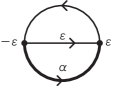
Let $c$ be a chord of a Gauss diagram $G$ with sign $\varepsilon=\varepsilon(c)$. We give signs $-\varepsilon$ and $\varepsilon$ to the initial and terminal endpoints of $c$, respectively. We consider the case that $G$ is circular. The endpoints of $c$ divide the circle into two arcs. Let $\alpha$ be the arc oriented from the initial endpoint of $c$ to the terminal. See Figure 1. The index of $c$ is the sum of signs of endpoints of chords on $\alpha$, and denoted by ${\rm Ind}_{G}(c)$ (cf. [1, 9, 11]). In the case that $G$ is linear, the index of $c$ is defined as that of $c$ in the closure of $G$.

Figure 1. The orientation and signs of a chord and its endpoints.

Let $G$ be a circular or linear Gauss diagram. For a positive integer $r$, we denote by $G^{(r)}$ the Gauss diagram obtained from $G$ by removing all the chords $c$ with ${\rm Ind}_{G}(c)\not\equiv 0~{}({\rm mod}\ r)$ (cf. [12]). In particular, we have $G^{(1)}=G$. For $r=0$, we denote by $G^{(0)}$ the Gauss diagram obtained from $G$ by removing all the chords $c$ with ${\rm Ind}_{G}(c)\neq 0$. Since the number of chords of $G$ is finite, we have $G^{(r)}=G^{(0)}$ for sufficiently large $r$.

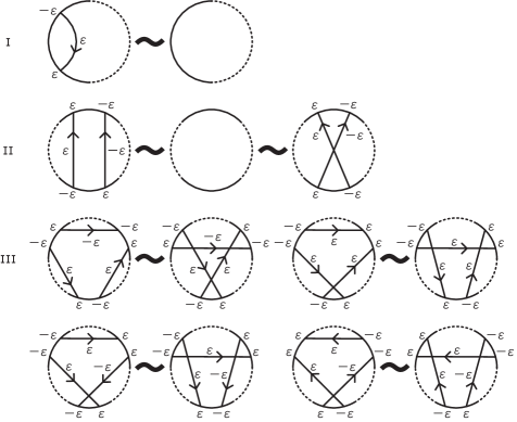
Two circular Gauss diagrams $G$ and $H$ are equivalent, denoted by $G\sim H$, if $G$ is related to $H$ by a finite sequence of Reidemeister moves I–III as shown in Figure 2. A virtual knot is an equivalence class of circular Gauss diagrams up to this equivalence relation (cf. [3, 8]). Similarly, the equivalence relation among linear Gauss diagrams are defined, and an equivalence class is called a long virtual knot. The trivial (long) virtual knot is presented by a Gauss diagram with no chord.

Figure 2. Reidemeister moves on Gauss diagrams.

Lemma 2.1 (cf. [5, 12]).

Let $G$ and $H$ be circular or linear Gauss diagrams such that $G\sim H$. Then it holds that $G^{(r)}\sim H^{(r)}$ for any integer $r\geq 0$. $\Box$

Although only the case of a circular Gauss diagram is studied in [5, 12], Lemma 2.1 for a liner Gauss diagram can be proved similarly.

Definition 2.2.

Let $K$ be a (long) virtual knot, and $r\geq 0$ an integer. The $r$-covering of $K$ is the (long) virtual knot presented by $G^{(r)}$ for some Gauss diagram $G$ of $K$. We denote it by $K^{(r)}$.

The well-definedness of $K^{(r)}$ follows from Lemma 2.1. We have $K^{(1)}=K$ and $K^{(r)}=K^{(0)}$ for sufficiently large $r$.

Let $c(G)$ denote the number of chords of a Gauss diagram $G$. The real crossing number of a (long) virtual knot $K$ is the minimal number of $c(G)$ for all Gauss diagrams $G$ of $K$, and denoted by ${\rm c}(K)$.

Lemma 2.3.

Let $K$ be a $($long$)$ virtual knot, and $r\geq 0$ an integer. Then it holds that ${\rm c}(K^{(r)})\leq{\rm c}(K)$. In particular, ${\rm c}(K^{(r)})={\rm c}(K)$ holds if and only if $K^{(r)}=K$.

Proof.

Let $G$ be a Gauss diagram of $K$ with $c(G)={\rm c}(K)$. Since $G^{(r)}$ is obtained from $G$ by removing some chords, we have

$${\rm c}(K^{(r)})\leq c(G^{(r)})\leq c(G)={\rm c}(K).$$

In particular, if the equality holds, then $G^{(r)}=G$ and $K^{(r)}=K$. ∎

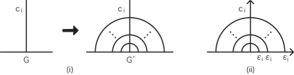
Let $c_{1},\dots,c_{n}$ be chords of a Gauss diagram $G$. We add several parallel chords near an endpoint of $c_{i}$ $(i=1,\dots,n)$ to obtain a Gauss diagram $G^{\prime}$. Here, the orientations and signs of the added chords are chosen arbitrarily. See Figure 3(i). The parallel chords added to $c_{i}$ are called anklets of $c_{i}$. We remark that the index of an anklet is equal to $\pm 1$.

Figure 3. Anklets.

Lemma 2.4.

Let $c_{1},\dots,c_{n}$ be chords of a Gauss diagram $G$. For any integers $a_{1},\dots,a_{n}$, by adding several anklets to each $c_{i}$ near its initial endpoint suitably, we obtain a Gauss diagram $G^{\prime}$ such that ${\rm Ind}_{G^{\prime}}(c_{i})=a_{i}$ for any $i=1,\dots,n$, and ${\rm Ind}_{G^{\prime}}(c)={\rm Ind}_{G}(c)$ for any $c\neq c_{1},\dots,c_{n}$.

Proof.

Put $d_{i}=a_{i}-{\rm Ind}_{G}(c_{i})$ for $i=1,\dots,n$. We add $|d_{i}|$ anklets to $c_{i}$ near its initial endpoint such that the signs of right endpoints of the anklets are equal to $\varepsilon_{i}$, where $\varepsilon_{i}$ is the sign of $d_{i}$. See Figure 3(ii).

Let $G^{\prime}$ be the obtained Gauss diagram. Then we have

$${\rm Ind}_{G^{\prime}}(c_{i})={\rm Ind}_{G}(c_{i})+\varepsilon_{i}|d_{i}|={\rm Ind}_{G}(c_{i})+d_{i}=a_{i}.$$

Furthermore the index of a chord other than $c_{1},\dots,c_{n}$ does not change. ∎

3. The $0$-covering $K^{(0)}$

For an integer $n\geq 2$, we define a map $f_{n}:\{2,3,\dots,n\}\rightarrow{\mathbb{Z}}$ which satisfies

$$\sum_{{r\leq i\leq n}\atop{i\equiv 0\ ({\rm mod}\ r)}}f_{n}(i)=-1$$

for any integer $r$ with $2\leq r\leq n$. The map $f_{n}$ exists uniquely. Put

$$P_{n}=\{i\mid 2\leq i\leq n,f_{n}(i)\neq 0\}.$$

Example 3.1.

For $n=10$, we have

$$\left\{\begin{array}[]{lrl}f_{10}(2)+f_{10}(4)+f_{10}(6)+f_{10}(8)+f_{10}(10)&=-1&\mbox{for }r=2,\\ f_{10}(3)+f_{10}(6)+f_{10}(9)&=-1&\mbox{for }r=3,\\ f_{10}(4)+f_{10}(8)&=-1&\mbox{for }r=4,\\ f_{10}(5)+f_{10}(10)&=-1&\mbox{for }r=5,\\ f_{10}(6)&=-1&\mbox{for }r=6,\\ f_{10}(7)&=-1&\mbox{for }r=7,\\ f_{10}(8)&=-1&\mbox{for }r=8,\\ f_{10}(9)&=-1&\mbox{for }r=9,\\ f_{10}(10)&=-1&\mbox{for }r=10.\end{array}\right.$$

Therefore we have

$$f_{10}(i)=\left\{\begin{array}[]{rl}2&(i=2),\\ 1&(i=3),\\ 0&(i=4,5),\\ -1&(6\leq i\leq 10)\end{array}\right.\mbox{ and }P_{10}=\{2,3,6,7,8,9,10\}.$$

Theorem 3.2.

For any integer $n\geq 1$ and long virtual knot $J$, there is a long virtual knot $K$ such that

$$K^{(r)}=\left\{\begin{array}[]{ll}J&\mbox{for }r=0\mbox{ and }r\geq n+1,\\ K&\mbox{for }r=1,\ and\\ O&\mbox{otherwise}.\\ \end{array}\right.$$

Here, $O$ denotes the trivial long virtual knot.

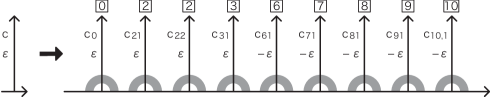
Proof.

Let $H$ be a linear Gauss diagram of $J$. We construct a linear Gauss diagram $G$ as follows: First, we replace each chord $c$ of $H$ by $1+\sum_{i\in P_{n}}|f_{n}(i)|$ parallel chords labeled $c_{0}$ and $c_{ij}$ for $i\in P_{n}$ and $1\leq j\leq|f_{n}(i)|$. The orientations of $c_{0}$ and $c_{ij}$’s are the same as that of $c$. The signs of them are given such that

• $\varepsilon(c_{0})=\varepsilon(c)$, and

• $\varepsilon(c_{ij})=\varepsilon(c)\delta_{i}$ for $i\in P_{n}$, where $\delta_{i}$ is the sign of $f_{n}(i)\neq 0$.

Next, we add several anklets to each of $c_{0}$ and $c_{ij}$’s such that

• ${\rm Ind}_{G}(c_{0})=0$, and

• ${\rm Ind}_{G}(c_{ij})=i$ for $i\in P_{n}$.

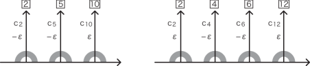
The obtained Gauss diagram is denoted by $G$.

Figure 4 shows the case $n=10$ replacing each chord $c$ of $H$ with nine chords $c_{0},c_{21},c_{22},c_{31},\dots,c_{10,1}$ and several anklets. The boxed numbers of the chords indicate their indices.

Figure 4. The case $n=10$.

By the conditions (i)–(iv), we have $G^{(0)}=H$; in fact, we remove the chords whose indices are non-zero from $G$ to obtain $G^{(0)}$. Similarly, we have $G^{(r)}=H$ for any $r\geq n+1$. Therefore it holds that $K^{(0)}=K^{(r)}=J$ for $r\geq n+1$.

For $2\leq r\leq n$, $G^{(r)}$ is obtained from $G$ by removing the chords whose indices are not divisible by $r$. In particular, all the anklets are removed. Among the chords $c_{0}$ and $c_{ij}$’s, the sum of signs of chords whose indices are divisible by $r$ is equal to

$$\varepsilon(c)+\varepsilon(c)\sum_{{r\leq i\leq n}\atop{i\equiv 0\ ({\rm mod}\ r)}}\delta_{i}|f_{n}(i)|=\varepsilon(c)+\varepsilon(c)\sum_{{r\leq i\leq n}\atop{i\equiv 0\ ({\rm mod}\ r)}}f_{n}(i)=0.$$

Therefore all the chords of $G^{(r)}$ can be canceled by Reidemesiter moves II so that $K^{(r)}$ is the trivial long virtual knot. ∎

4. The $r$-covering $K^{(r)}$ for $r\geq 2$

For an integer $n\geq 2$, we define a map $g_{n}:\{2,3,\dots,n\}\rightarrow{\mathbb{Z}}$ which satisfies

$$g_{n}(n)=1\mbox{ and }\sum_{{r\leq i\leq n}\atop{i\equiv 0\ ({\rm mod}\ r)}}g_{n}(i)=0$$

for any integer $r$ with $2\leq r<n$. The map $g_{n}$ exists uniquely. Put

$$Q_{n}=\{i\mid 2\leq i\leq n,g_{n}(i)\neq 0\}.$$

Example 4.1.

(i) For $n=10$, it holds that

$$\left\{\begin{array}[]{lrl}g_{10}(2)+g_{10}(4)+g_{10}(6)+g_{10}(8)+g_{10}(10)&=0&\mbox{for }r=2,\\ g_{10}(3)+g_{10}(6)+g_{10}(9)&=0&\mbox{for }r=3,\\ g_{10}(4)+g_{10}(8)&=0&\mbox{for }r=4,\\ g_{10}(5)+g_{10}(10)&=0&\mbox{for }r=5,\\ g_{10}(6)&=0&\mbox{for }r=6,\\ g_{10}(7)&=0&\mbox{for }r=7,\\ g_{10}(8)&=0&\mbox{for }r=8,\\ g_{10}(9)&=0&\mbox{for }r=9,\\ g_{10}(10)&=1&\mbox{for }r=10.\end{array}\right.$$

Therefore we have

$$g_{10}(i)=\left\{\begin{array}[]{rl}1&(i=10),\\ -1&(i=2,5),\\ 0&({\rm otherwise}),\\ \end{array}\right.\mbox{ and }Q_{10}=\{2,5,10\}.$$

(ii) For $n=12$, we have

$$g_{12}(i)=\left\{\begin{array}[]{rl}1&(i=2,12),\\ -1&(i=4,6),\\ 0&({\rm otherwise}),\\ \end{array}\right.\mbox{ and }Q_{12}=\{2,4,6,12\}.$$

Theorem 4.2.

For any integer $n\geq 2$ and long virtual knot $J$, there is a long virtual knot $K$ such that

$$K^{(r)}=\left\{\begin{array}[]{ll}J&\mbox{for }r=n,\\ K&\mbox{for }r=1,\ and\\ O&\mbox{otherwise}.\\ \end{array}\right.$$

Proof.

The proof is similar to that of Theorem 3.2 by using $g_{n}$ instead of $f_{n}$. Let $H$ be a linear Gauss diagram of $J$. We construct a linear Gauss diagram $G$ of $K$ as follows: First, we replace each chord $c$ of $H$ by $\sum_{i\in Q_{n}}|g_{n}(i)|$ parallel chords labeled $c_{i}$ for $i\in Q_{n}$. The orientations of $c_{i}$’s are the same as that of $c$. The signs of them are given such that $\varepsilon(c_{i})=\varepsilon(c)\delta_{i}$, where $\delta_{i}$ is the sign of $g_{n}(i)\neq 0$. Next, we add several anklets to each of $c_{i}$’s such that ${\rm Ind}_{G}(c_{i})=i$ for $i\in Q_{n}$. 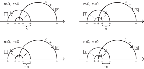The obtained Gauss diagram is denoted by $G$.

In the left of Figure 5, we shows the case $n=10$ replacing each chord $c$ of $H$ with three chords $c_{2},c_{5},c_{10}$ and several anklets. In the right figure, the case of $n=12$ is given.

Figure 5. The cases $n=10$ and $12$.

Since any chord $c$ of $G$ satisfies $1\leq|{\rm Ind}_{G}(c)|\leq n$, we obtain $G^{(0)}$ and $G^{(r)}$ for $r\geq n+1$ by removing all the chords from $G$.

For $2\leq r<n$, $G^{(r)}$ is obtained from $G$ by removing the chords whose indices are not divisible by $r$. Among the chords $c_{i}$’s, the sum of signs of chords whose indices are divisible by $r$ is equal to

$$\varepsilon(c)\sum_{{r\leq i\leq n}\atop{i\equiv 0\ ({\rm mod}\ r)}}\delta_{i}|g_{n}(i)|=\varepsilon(c)\sum_{{r\leq i\leq n}\atop{i\equiv 0\ ({\rm mod}\ r)}}g_{n}(i)=0.$$

Therefore all the chords of $G^{(r)}$ can be canceled by Reidemeister moves II so that $K^{(r)}$ is the trivial long virtual knot.

Finally, for $r=n$, we have $G^{(n)}=H$ by definition immediately. ∎

We see that $g_{n}$ is coincident with a famous function as follows.

Proposition 4.3.

Let $\mu$ be the Möbius function. Then we have

$$g_{n}(i)=\left\{\begin{array}[]{cl}\mu(\frac{n}{i})&\mbox{if $n$ is divisible by $i$, and}\\ 0&\mbox{otherwise}.\end{array}\right.$$

Proof.

Let $h_{n}(i)$ be the right hand side of the equation in the proposition. Since $h_{n}(n)=\mu(1)=1=g_{n}(n)$, it is sufficient to prove that

$$\sum_{{r\leq i\leq n}\atop{i\equiv 0\ ({\rm mod}\ r)}}h_{n}(i)=0$$

for any integer $r$ with $2\leq r<n$.

Assume that $n$ is not divisible by $r$. Then $n$ is not divisible by any $i$ such that $r\leq i\leq n$ and $i\equiv 0$ (mod $r$). Therefore we have

$$\sum_{{r\leq i\leq n}\atop{i\equiv 0\ ({\rm mod}\ r)}}h_{n}(i)=\sum_{{r\leq i\leq n}\atop{i\equiv 0\ ({\rm mod}\ r)}}0=0.$$

Assume that $n$ is divisible by $r$. By the property of the Möbius function, it holds that

$$\sum_{{r\leq i\leq n}\atop{i\equiv 0\ ({\rm mod}\ r)}}h_{n}(i)=\sum_{r|i|n}\mu(\frac{n}{i})=\sum_{d|\frac{n}{r}}\mu(d)=0.$$

Therefore we have $g_{n}=h_{n}$. ∎

5. The writhe polynomial

For an integer $n\neq 0$ and a sign $\varepsilon=\pm 1$, the $(n,\varepsilon)$-snail is a linear Gauss diagram consisting of a chord $c$ with $\varepsilon(c)=\varepsilon$ and $|n|$ anklets such that the indices of $c$ and each anklet are equal to $n$ and $1$, respectively. See Figure 6.

Figure 6. The snail $S(n,\varepsilon)$.

Let $G$ be a Gauss diagram of a (long) virtual knot $K$. For an integer $n\neq 0$, we denote by $w_{n}(G)$ the sum of signs of all chords $c$ of $G$ with ${\rm Ind}_{G}(c)=n$. Then $w_{n}(G)$ does not depend on a particular choice of $G$ of $K$; that is, $w_{n}(G)$ is an invariant of $K$. In [11], the proof is given for a virtual knot, and the case of a long virtual knot is similarly proved. It is called the $n$-writhe of $K$ and denoted by $w_{n}(K)$. The writhe polynomial of $K$ is defined by

$$W_{K}(t)=\sum_{n\neq 0}w_{n}(K)t^{n}-\sum_{n\neq 0}w_{n}(K)\in{\mathbb{Z}}[t,t^{-1}].$$

This invariant was introduced in several papers [2, 9, 11] independently.

Theorem 5.1.

Let $J$ be a long virtual knot, and $f(t)\in{\mathbb{Z}}[t,t^{-1}]$ a Laurent polynomial with $f(1)=f^{\prime}(1)=0$. Then there is a long virtual knot $K$ such that

• $K^{(r)}=J^{(r)}$ for any integer $r=0$ and $r\geq 2$, and

• $W_{K}(t)=f(t)$.

Proof.

Put $g(t)=f(t)-W_{J}(t)=\sum_{n\in{\mathbb{Z}}}a_{n}t^{n}$. By Theorem 1.1, we have $g(1)=g^{\prime}(1)=0$. Therefore it holds that $a_{0}=\sum_{n\neq 0,1}(n-1)a_{n}$ and $a_{1}=-\sum_{n\neq 0,1}na_{n}$.

Let $H$ be a linear Gauss diagram of $J$. We construct a linear Gauss diagram $G$ by juxtaposing $H$ and $|a_{n}|$ copies of $S(n,\varepsilon_{n})$ for every integer $n$ with $n\neq 0,1$ and $a_{n}\neq 0$. Here, $\varepsilon_{n}$ is the sign of $a_{n}\neq 0$.

Let $K$ be the long virtual knot presented by $G$. The contribution of each snail $S(n,\varepsilon_{n})$ to the writhe polynomial $W_{K}(t)$ is equal to $\varepsilon_{n}t^{n}-\varepsilon_{n}nt+\varepsilon_{n}(n-1)$. Therefore it holds that

$$W_{K}(t) = W_{J}(t)+\sum_{n\neq 0,1}|a_{n}|\bigr{(}\varepsilon_{n}t^{n}-\varepsilon_{n}nt+\varepsilon_{n}(n-1)\bigr{)}$$

$$= W_{J}(t)+\sum_{n\neq 0,1}a_{n}\bigr{(}t^{n}-nt+(n-1)\bigr{)}$$

$$= W_{J}(t)+g(t)=f(t).$$

By definition, $S(n,\varepsilon_{n})^{(r)}$ has the only chord $c$ if $n$ is divisible by $r$. Otherwise it has no chord. Therefore $G^{(r)}$ is equivalent to $H^{(r)}$, and hence $K^{(r)}=J^{(r)}$ for any integer $r=0$ and $r\geq 2$. ∎

Theorem 5.2.

Let $m\geq 1$ be an integer, $J_{n}$ $(0\leq n\leq m,n\neq 1)$ $m$ long virtual knots, and $f(t)$ a Laurent polynomial with $f(1)=f^{\prime}(1)=0$. Then there is a long virtual knot $K$ such that

$$K^{(r)}=\left\{\begin{array}[]{ll}J_{0}&\mbox{for }r=0\mbox{ and }r\geq m+1,\\ K&\mbox{for }r=1,\\ J_{r}&\mbox{otherwise},\\ \end{array}\right.$$

and $W_{K}(t)=f(t)$.

Proof.

Let $K_{0}$ be a long virtual knot obtained by applying Theorem 3.2 to the pair of $m$ and $J_{0}$. Let $K_{n}$ be a long virtual knot obtained by applying Theorem  4.2 to each pair of $n$ and $J_{n}$ $(2\leq n\leq m)$. We juxtapose $K_{0},K_{2},\dots,K_{m}$ to have a long virtual knot $K^{\prime}$. Let $K$ be a long virtual knot obtained by applying Theorem 5.1 to the pair of $K^{\prime}$ and $f(t)$. Then we see that $K$ is a desired long virtual knot. ∎

Proof of Theorem 1.2.

Let $J_{n}^{\circ}$ be a long virtual knot whose closure is $J_{n}$ $(0\leq n\leq m,n\neq 1)$. Let $K^{\circ}$ be a long virtual knot obtained by applying Theorem 5.2. Then we see that the closure of $K^{\circ}$ is a desired virtual knot. ∎