OCU-PHYS 490
AP-GR 150
Perfect Charge Screening of Extended Sources
in an Abelian-Higgs Model
Abstract
We investigate a classical system that consists of a U(1) gauge field and a complex Higgs scalar field with a potential that breaks the symmetry spontaneously. We obtain numerical solutions of the system in the presence of a smoothly extended external source with a finite size. In the case of the source is spread wider than the mass scale of the gauge field, perfect screening of the external source occurs, namely, charge density of the source is canceled out everywhere by induced counter charge density cloud of the scalar and vector fields. Energy density induced by the cloud is also obtained.
I Introduction
Gauge theories are fundamental frameworks in modern physics for description of the interactions in nature. In a model where the gauge symmetry is spontaneously broken, the vector gauge field that acquires a mass mediates a short-range force. The massive vector field around a source charge drops off exponentially with the mass scale, then the influence of the source charge by the massive vector field is limited in a finite range of distance. In other words, the source charge should be screened by some appropriate configuration of the fields.
Motivated by color confinement, charge screening was investigated in scalar electrodynamics Mandula1977 ; Adler_Piran ; Bawin_Cugnon , and Yang-Mills theories Sikivie_Weiss ; William . It was reported that there exist minimum energy solutions which describe the screening of an external source charge in gauge field models Mandula1977 ; Bawin_Cugnon ; Adler_Piran ; Sikivie_Weiss ; William .
In most of these works, singular shells are assumed as the source charge for convenience of analysis. Smoothly extended charged objects with finite support are also possible sources to be screened. As examples of the extended charged objects, we can consider non-topological solitons, which are studied in coupled scalar fields systems Friedberg_Lee_Sirlin , and a complex scalar field with non-trivial self-interaction systems Coleman . Non-topological solitons of complex scalar fields coupled with a gauge field are also investigated Lee_Stein-Schabes_Watkins_Widrow ; Shi_Li ; Gulamov_etal .
We study, in this paper, screening of a smoothly extended source in a system consisting of a U(1) gauge field and a complex Higgs scalar field with a potential that causes spontaneous symmetry breaking. The purpose of this paper is to clarify local configuration of the fields that screens the extended source, in detail. We solve a coupled field equations numerically, and obtain spherically symmetric static solutions where the charge screening occurs. We show that external charge is perfectly screened, that is, the charge is canceled out everywhere by counter charge induced by the vector and scalar fields, if the external charge spread widely compare to the mass scale of the vector field.
The organization of this paper is as follows. In the next section, we present the basic system that is analyzed. In section III, we reduce the system by assuming symmetry on the system, and set up external sources and boundary conditions. Then, we obtain a set of ordinary differential equations to be solved. In section IV, we perform numerical integrations of the equations in various cases for the external sources, and show how the extended sources are screened. Section V is devoted to summary and discussion.
II Basic System
We consider an abelian Higgs system described by the Lagrangian density
| (1) |
where is the field strength of a U(1) gauge field , and is a complex Higgs scalar field with the potential
| (2) |
where and are positive constants. The Higgs field couples to the gauge field by the covariant derivative given by
| (3) |
where is a coupling constant. The Lagrangian density (1) is invariant under local U(1) gauge transformations,
| (4) | ||||
| (5) |
where is an arbitrary function.
The energy of the system is given by
| (6) |
where , , and denotes spatial index. In the vacuum state, which minimizes the energy (6), and should take the form
| (7) |
where is an arbitrary function. Equivalently, eliminating we have
| (8) |
After the Higgs scalar field takes the vacuum expectation value , the gauge field absorbing the Nambu-Goldstone mode, the phase of , forms a massive vector field with the mass , and the real scalar field that denotes a fluctuation of the amplitude of around acquires the mass .
In order to study the charge screening, adding an extremal source current, , coupled with to the original Lagrangian (1), we consider the action111 The case of vanishing potential, , in which the symmetry does not break, is studied in ref.Mandula1977 , and the case , in which partial screening occurs, is studied in ref.Bawin_Cugnon .
| (9) |
By varying (9) with respect to and , we obtain the equations of motion
| (10) | |||
| (11) |
where is the gauge invariant current density that consists of and defined by
| (12) |
III Spherically symmetric model
We consider a spherically symmetric and static external source in the form
| (13) |
where and are the time and the radial coordinates. We also assume that the fields are spherically symmetric and stationary in the form,
| (14) | ||||
| (15) |
where is a constant, and is a real function of . By using the gauge transformation (4) and (5) to incorporate the phase rotation of , i.e., Nambu-Goldstone mode, with , we introduce a new variable as
| (16) |
The charge density induced by the fields and defined by (12) is written as
| (17) |
Using the ansatz (14) and (15), we rewrite the energy (6) for the symmetric system as
| (20) | |||
| (21) |
where
| (22) | |||
| (23) |
are density of kinetic energy, elastic energy, potential energy, and electrostatic energy, respectively.
We consider a point source case, where the charge density is given by the -function as
| (24) |
where denotes the total external charge, and two extended source cases separately. As the extended source cases, we discuss Gaussian distribution sources and homogeneous ball sources. The both are smoothly distributed and have finite supports.
The charge density of the Gaussian distribution source is given by
| (25) |
where is the width of the extended source. The total external charge is assumed to be normalized as
| (26) |
then the central density is given by
| (27) |
In the limit , the charge density (25) with (27) reduces to the point source case (24).
The charge density of the homogeneous ball considered in this paper is given by
| (28) |
where is the radius of the external source, and is the thickness of surface of the ball. We assume so that the charge density within the radius is almost constant value . Then, the total external charge is in this case.
We impose boundary conditions so that the fields are regular at the origin. The regularity conditions for the spherically symmetric fields at the origin are
| (29) |
The energy density at the origin is finite for finite central values of and . At infinity, the fields should be in the vacuum state, which minimizes in (21). Therefore, we impose the conditions
| (30) |
IV Numerical Calculations
We use the relaxation method to obtain numerical solutions to the coupled ordinary differential equations (18) and (19). In numerics, hereafter, we set , and scale the radial coordinate as , and scale the functions , as , , respectively.
IV.1 Point source
Before the case of smoothly extended external charge distributions, we consider the case of a point source (24), in which asymptotic behavior of the fields near the source is known analytically. Main purposes of this subsection are confirmation of our numerical calculation and observation of basic properties of the solutions. We set and so that and .
As is shown in Appendix A, inspecting the equations (18) and (19), we obtain the asymptotic behavior of and near the origin are given by
| (31) |
and
| (32) |
where , , , and are constants. We should note that the behavior of critically depends on the parameter .
On the other hand, the asymptotic behaviors at infinity are given by
| (33) | ||||
| (34) |
where and are constants.
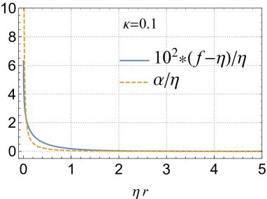
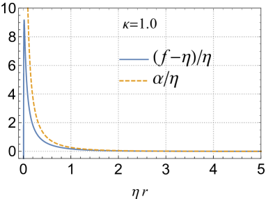
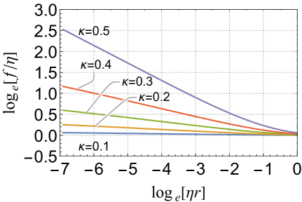
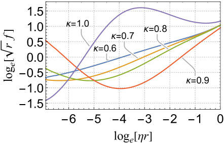
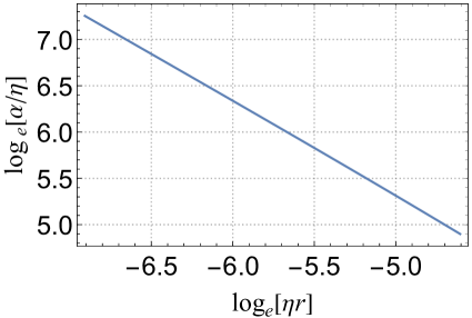
Here, we solve equations (18) and (19) numerically, and study basic properties of the system. Typical behaviors of the functions and are shown in Fig.1. Especially, the behaviors of and near the origin are shown in Fig.2. In the case of , is given by the power function of , while in the case of , oscillatory behaviors appear. The function is in proportion to independent with . These behaviors coincide with (31) and (32). The asymptotic behaviors of the functions and in a distant region coincide with (33) and (34) as shown in Fig.3.
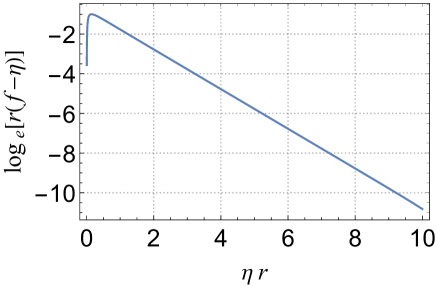
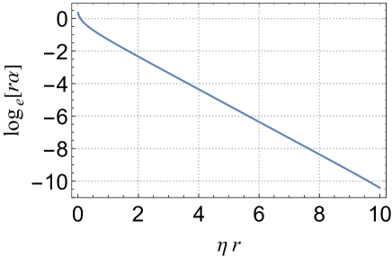
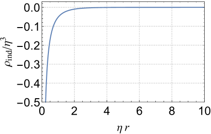
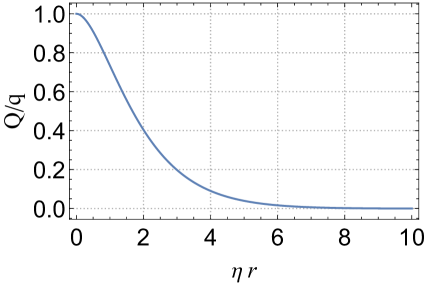
The induced charge density in (17) is plotted in the left panel of Fig.4 as a function of . The induced charge, whose sign is opposite to the external source charge, distributes as a cloud around the point charge source. We define the total charge within the radius , say , by
| (35) |
where the total charge density is defined by
| (36) |
As shown in Fig.4, is monotonically decreasing function of . It means that the positive charge of the external source is screened by the induced negative charge cloud. In the region near the point source the charge is partly screened, i.e., and at a large distance the charge is totally screened, i.e., .
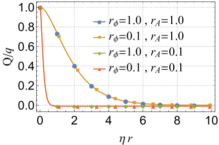
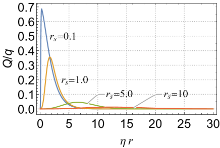
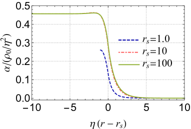
For some sets of two characteristic length scales , the function is plotted in Fig.5. We see that the shape of does not depend on , while the width of is given by . In any case, in a distant region where , charge is totally screened. Except the neighborhood of the origin, as shown in Fig.1, takes the vacuum expectation value . The massive gauge mode with mass causes the charge screening, with the size of .
IV.2 Gaussian distribution source
For the first example of smoothly extended source, we consider the external charge density given by the Gaussian distribution (25). As the boundary conditions, we impose the regularity conditions (29) at the origin, and the vacuum condition (30) at infinity.
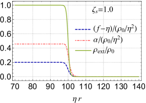
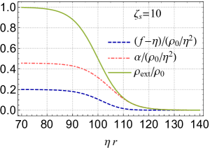
For the extended external sources, the behaviors of and do not depend critically on the value of unlike the point source case. So, we concentrate on the case , i.e., . We fix , , and perform numerical calculation with several values of that denotes the thickness of the external source.
IV.2.1 Field configurations
By numerical calculations, we show typical behaviors of the function and with the external charge density in the cases of , and in Fig.6. We see that the function and change in their shapes with . Especially, for the thin source case, , numerical solutions are shown in Fig.7. As approaches to zero, since the normalized Gaussian function (25) with (27) reduces to the -function (24), then as we expected, the function and approach to the solutions for the point source case discussed in the previous subsection. In the thick source case, , the widths of and are order of . Typical behaviors can be understood by analytical method given in Appendix B.
IV.2.2 Charge screening
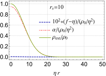
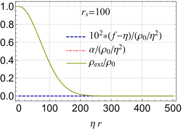
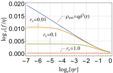
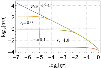
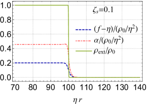
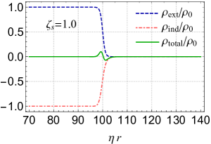
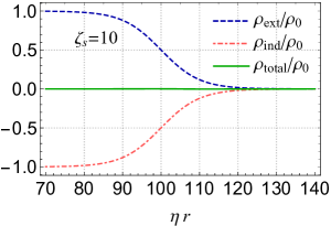
We depict the induced charge density with the external charge density in Fig.8. The sign of is opposite to . In the central region of and cases, we find that is larger than , i.e., total charge density has the same sign with . As increases, exceeds . In the region , the both and decrease quickly to zero. As shown in Fig.9, , the total charge within radius , decreases to zero in the region , it means the external charge is totally screened by the induced charge cloud for a distant observer.
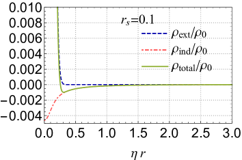
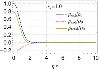
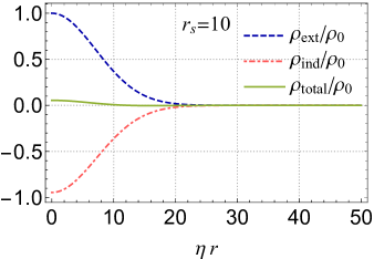
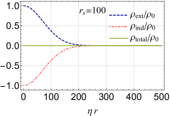
In the case of , the width of the induces charge cloud is the order of , while in the case of , the width is almost same as . In the case of , we have
| (37) |
as is justified by (66). Then, vanishes everywhere, equivalently vanishes everywhere. We call this ‘perfect screening’.
IV.2.3 Energy of the cloud
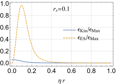
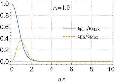
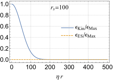
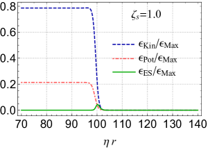
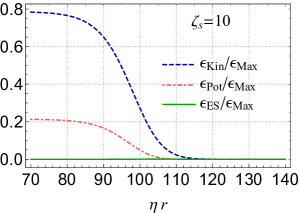
We inspect the energy density of the numerical solutions. The components of energy density given by (22) and (23) are shown in Fig.10. The dominant components of energy density are and , while and are negligibly small in the present cases.
In the thin source case, , the electrostatic energy density dominates the total energy density (see case in the first panel of Fig.10 for example), i.e.,
| (38) |
In the near region , as shown in Appendix B, the asymptotic behavior of the function near the origin is given by (63), i.e.,
| (39) |
where is the central value of . Substituting (39) into (38), the energy within is given by
| (40) |
In the region , since is given by (33), then the energy of the system (20) in this range can be written by
| (41) | ||||
| (42) |
Therefore, the total energy is proportional to .
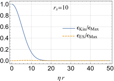
In contrast, in a thick source case, , as shown in (68) of Appendix B, we see that and , then the energy density becomes
| (43) |
Therefore, the energy given by
| (44) |
is proportional to .
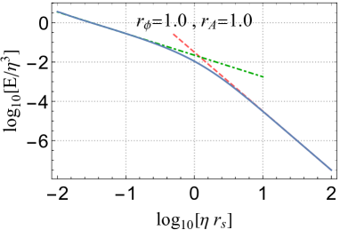
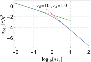

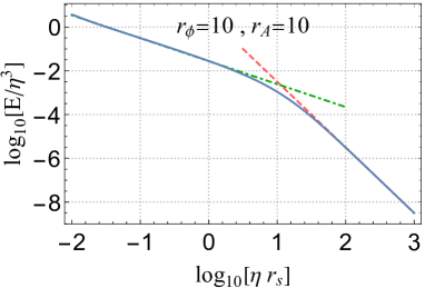
By numerical calculations for some values of the parameter sets , , the energy is plotted as a function of in Fig.11. In all cases, we see that for small , and for large . The power index changes around .
IV.3 Homogenious ball source
As the second example of smoothly extended source, we consider the ball of constant charge density expressed by (28). As same as the Gaussian distribution case discussed above, we set , and . We fix the central charge density , and find numerical solutions for several values of , radius of the ball, and , surface thickness parameter. Note that the total external charge is in proportion to .
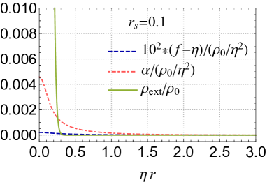
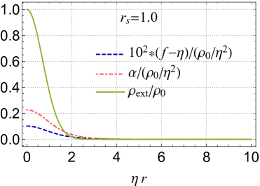
By numerical calculations, and with are shown in the cases of , and for fixed surface thickness as in Fig.12. As is shown in AppendixC, in the region , where , we see
| (45) |
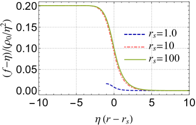
where and are constants given in AppendixC. In the region , where , we see simply and . The functions and change the values quickly in the vicinity of the ball surface . The profiles of and near the ball surface are almost identical if (see Fig.13 ).
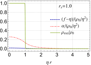
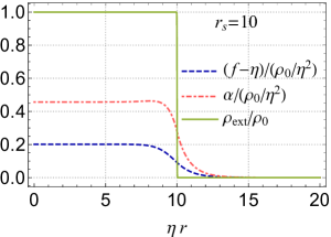
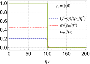
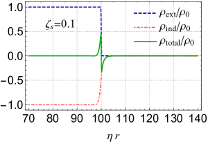
Next, we consider variation of surface thickness for fixed ball radius . The profile of the functions and , the charge density, and energy density are shown in the cases of , and for fixed ball radius as in Fig.12. Inside the homogeneous ball source, the induced charge density cancels the external charge density except the vicinity of the ball surface. In the thin ball surface case, , at the surface, where changes its value quickly, the induced charge exceeds the external charge inside the surface, and vice versa outside. Therefore, an electric double layer emerges at the surface of the ball. For the thick surface case, , charge cancellation occur everywhere even at the surface. Namely, the perfect screening occurs in this case.
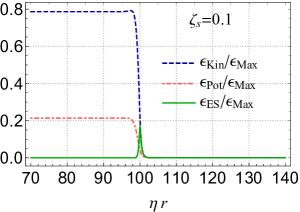
The components of energy density given in (22) and (23) are shown in Fig.14. Inside the homogeneous ball, the kinetic energy dominate the energy density and the electrostatic energy density caused by the electric double layer appears at the neighborhood of surface for the thin surface case.
V Summary and Discussion
In this paper, we have studied the classical system that consists of a U(1) gauge field and a complex Higgs scalar field with a potential that breaks the symmetry spontaneously. We have presented numerical solutions in the presence of a smoothly extended external source with a finite size. Owing to the existence of the external source, counter charge cloud is induced by the scalar and the vector fields.
We have investigated two extended external sources: Gaussian distribution sources and homogeneous ball sources. In the case of Gaussian distribution source, the profile of the total charge within radius , , depends on the width of the external source, . In the thin source case, where is much smaller than the mass scale of the vector field, , non-vanishing peak of appears at a radius in the range . Then, the charge density is detectable in the region . The maximum value of is less than the total external charge, then the partial screening occurs in a finite distance. As increases, damps quickly, then the total charge screening occurs by the induced charge cloud for a distant observer. In the thick source case, where is much larger than , is almost zero everywhere, equivalently, almost vanishes everywhere. In this case, the charge is perfectly screened so that the charge is not detectable anywhere.
In accordance with the induced charge cloud, the energy density of the fields is also induced around the external source. In the thin source case, the electrostatic energy produced by the non-vanishing total charge density appears dominantly. In the thick source case, the kinetic energy, square of covariant time derivative of the scalar field, dominates the energy density. The total energy of the cloud depends on the thickness parameter ; for the thin source, is proportional to , while for the thick source, is proportional to . The transition of the power index occur at .
For the homogeneous ball source, we have considered that the charge density is constant within the ball radius, , which is assumed to be much larger than , and the charge density varies with the surface thickness scale, , at the ball surface. We found that inside the ball, , the amplitude of the scalar field and the gauge field take constant values, respectively, and outside the ball, , the scalar field takes the vacuum expectation value and the gauge field vanishes. At the ball surface, the both fields change their values quickly. The external charge is canceled out by the induced charge cloud except the vicinity of ball surface. In the thin surface case, , electric double layer appears at the ball surface. In the thick surface case, , the charge cancellation occurs even at the ball surface, namely, the perfect screening occurs.
The kinetic energy and the potential are main components of the energy density inside the ball. For the thin surface case, the electrostatic component of the energy density by the electric double layer appears at the ball surface.
In this paper, we have concentrated on the screening mechanism of external charge sources. It is interesting that the external sources are replaced by charged non-topological solitons. There exist non-topological soliton solutions of a complex scalar field where the conserved charges are extended smoothly. Can we expect the charge screening occurs on the non-topological solitons ?
In the studies of the non-topological solitons, typical profiles of charge density of solitons are Gaussian distributions and homogeneous balls Friedberg_Lee_Sirlin ; Coleman . Ungauged non-topological solitons are allowed to have infinitely large mass Lee_Stein-Schabes_Watkins_Widrow , while gauged solitons have upper limit of mass owing to repulsive force between charges Lee_Stein-Schabes_Watkins_Widrow ; Shi_Li . If a non-topological soliton exists in a system consisting of a complex field, a Higgs scalar field, and a U(1) gauge field, the charge screening of the soliton occurs as discussed in the present paper. It would be expected that the charge screened soliton has a infinitely large mass. If the solitons are spread wider than the mass scale of the gauge field, the perfect screening would occur. This is a preferable property for dark matter in the universe. We would report the existence of charge screened non-topological solitons, which would be an interesting candidate for the dark matter, in the forthcoming paper Ishihara_Ogawa .
Acknowledgements
We would like to thank Dr. K.-i. Nakao, Dr. N. Maru, and Dr. R. Nishikawa for valuable discussion. H.I. was supported by JSPS KAKENHI Grant Number 16K05358.
Appendix A Asymptotic behaviors for the point source
We analyze asymptotic behaviors of the scalar and gauge fields governed by (18) and (19) for a point source (24) Landau . The equations admit an exact solution and , the Coulomb solution. However, this configuration does not minimize the energy (20), i.e., not the vacuum. To seek other solutions with non-vanishing , we discuss asymptotic behavior of the fields near the point source and at infinity.
A.1 Near the point source
We assume that the asymptotic behavior of the fields in the vicinity of the point source are given by
| (46) | |||
| (47) |
where and are non-vanishing constants. Substituting these expression in (18) and (19), we obtain
| (48) | |||
| (49) |
First, we consider the case of . In this case, we can ignore the third term in (49), and obtain . By Gauss’ integral theorem applied in a small volume including the point source, we have
| (50) |
Since and , the first three terms in (48) should compensate each other. Then, we obtain
| (51) |
where .
If , is real number. For the upper sign in (51), the elastic energy density defined in (22) is finite in the limit , however it diverges for the lower sign. Then, we take the positive sign in (51) for the power index of .
If , becomes complex numbers
| (52) |
then we have the real function in the form
| (53) | ||||
| (54) |
where and are constants.
In the case of , after some consideration, we see should vanish. Then, it is not the case in which the expected solution exists.
A.2 Distant region
At spatial infinity, approaches to zero, and does to asymptotically. Then, in the distant region, we rewrite as
| (55) |
where as . Substituting (55) to (18) and (19), we obtain a set of linear differential equations
| (56) | |||
| (57) |
where higher order terms in and are neglected. Solving these equations, we obtain asymptotic behaviors of the functions as
| (58) | |||
| (59) |
where and are constants. These behaviors at the large distance are general if the external source has a compact support around the origin.
Appendix B Approximate solutions for the Gaussian distribution sources
First, we consider the thin source case, . As shown in the first panel of Fig.6 and Fig.8 for the case as an example, we see
| (60) |
in the near region, . Then, (18) and (19) reduces to
| (61) | |||
| (62) |
in this region. We easily find a set of approximate solutions that satisfies the boundary condition (29) in the expansion form
| (63) | |||
| (64) |
where and .
In the far region, , the functions and take the same forms of the point source case. The constants and should be adjusted so that the solutions are smoothly connected from the near region to the far region.
Next, we consider the thick source case, . Since the source is spread widely, the variation of the external charge density is very small. Accordingly, the variation of the functions and are also small as is seen in the last panel of Fig.6 as an example. Then the derivative terms in (18) and (19) can be negligible, and we have
| (65) | |||
| (66) |
If the external charge density is small such that
| (67) |
we have
| (68) |
This behavior is seen in the last panel of Fig.6.
Appendix C Approximate solutions for the homogeneous ball sources
In the homogeneous ball sources with , except the vicinity of the ball surface, , and are almost constants. We can approach approximately to this simple behaviors.
In the region , where , since the derivative terms in (19) and (18) can be ignored for the solutions that satisfy the boundary condition (29), then and take constant values. The equations of motion reduce to
| (69) | |||
| (70) |
By solving these coupled algebraic equations, we obtain
| (71) | ||||
| (72) |
where is the constant defined by
| (73) |
In the region , where , we have simply and . The fields and change their values quickly in the vicinity of the ball surface.
If , a global solution can be obtained approximately. In this case, as same as the Gaussian source case, . Moreover, if , the equation of the gauge field can be reduced to
| (74) |
where . This is the Proca equation for a homogenious ball source.
References
- (1) J. E. Mandula, Phys. Lett. 69B, 495 (1977).
- (2) S. L. Adler and T. Piran, Rev. Mod. Phys. 56, 1 (1984).
- (3) M. Bawin and J. Cugnon, Phys. Rev. D 37, 2344 (1988).
- (4) P. Sikivie and N. Weiss, Phys. Rev. Lett. 40, 1411 (1978).
- (5) W. B. Campbell and R. E. Norton, Phys. Rev. D 44, 3931 (1991).
- (6) R. Friedberg, T. D. Lee and A. Sirlin, Phys. Rev. D 13, 2739 (1976).
- (7) S. R. Coleman, Nucl. Phys. B 262, 263 (1985) Erratum: [Nucl. Phys. B 269, 744 (1986)].
- (8) K. M. Lee, J. A. Stein-Schabes, R. Watkins and L. M. Widrow, Phys. Rev. D 39, 1665 (1989).
- (9) X. Shi and X. Z. Li, J. Phys. A 24, 4075 (1991).
- (10) I. E. Gulamov, E. Y. Nugaev, A. G. Panin and M. N. Smolyakov, Phys. Rev. D 92, no. 4, 045011 (2015)
- (11) H. Ishihara and T. Ogawa, In preparation.
- (12) L.D. Landau and E.M. Lifschitz, “Quantum mechanics”, Pergamon Press (1965)