The Gromov-Hausdorff propinquity for metric Spectral Triples

Abstract.

We define a metric on the class of metric spectral triples, which is null exactly between unitarily equivalent spectral triples. This metric dominates the propinquity, and thus implies metric convergence of the quantum compact metric spaces induced by metric spectral triples. In the process of our construction, we also introduce the covariant modular propinquity, as a key component for the definition of the spectral propinquity.

1. Introduction

The primary purpose of our research is to bring forth a new approach to problems from mathematical physics and noncommutative geometry by constructing an analytic framework around Gromov-Hausdorff-like hypertopologies on classes of quantum spaces. The central themes of this project have been the construction of noncommutative analogues of the Gromov-Hausdorff distance [15, 16] adapted to C*-algebras [24, 31, 28, 26, 33, 32, 29, 27] and the initiation and advancement of a theory of metric convergence for various structures over $C^{\ast}$-algebras, such as modules [36, 39, 37] and group actions [34, 38, 35]. The present work introduces a distance on the space of metric spectral triples, strongly motivated by potential applications to mathematical physics, such as the convergence of matrix models to some limit [40].

Our motivation for this project emerges from four connected observations. First, a recurrent theme in mathematical physics is the construction of quantum models as limits of some discrete, often even finite models, when some metric on the spaces are involved. Second, certain approaches to quantum cosmology and quantum gravity involve an as-of-yet not fully understood geometry on the space of all space-times [55]. Notably, the first occurrence and study of the Gromov-Hausdorff distance was actually due to Edwards [13], motivated by Wheeler’s superspace approach to quantum gravity. Third, a set of converging ideas in quantum physics suggests the possibility that at the Planck scale, space-time may be best described as a noncommutative space [12], and metric considerations have become a component of this research, including many references to our work [53, 14, 11]. Fourth, remarkable new developments in geometry arose from the use of the Gromov-Hausdorff distance and the metric properties of manifolds and related spaces. We thus aim at developing a theory which allow us to formalize physics problems and problems from noncommutative geometry at the level of hyperspaces of quantum metric spaces and spectral triples, so as to apply to them new analytic techniques.

Spectral triples, as introduced by Connes [8, 9] as early as 1985 in his lectures at the Collège de France, have emerged as the preferred means to generalize Riemannian geometry to the noncommutative realm. Their importance lies in their well-established power in generalizing, in particular, spectral geometry to various new situations, from the study of the spaces of leaves of foliations, to defining a geometry on quantum tori, quantum spheres, and other quantum spaces, which, in turn, have found applications in mathematical physics. Our perspective on spectral triples provides a new direction for investigation, by focusing on the metric aspects of noncommutative geometry, and studying spaces of spectral triples.

The importance of our work in this paper is to be found in the applications it opens. Our present work puts a topology on the class of all metric spectral triples. Therefore, it becomes possible to address questions such as perturbations of metric within an analytical framework — quantifying the scale of perturbations, including the effects of changes of underlying topologies, and studying topological properties of classes of quantum spaces obtained from perturbations, such as compactness [27, 2, 32]. We can also discuss approximations of spectral triples by other spectral triples, for instance spectral triples on matrix models approximating spectral triples on infinite dimensional C*-algebras [26] — for instance, physically motivated models over fuzzy tori converging to quantum torus [40]. We can also discuss time evolution of quantum geometries, or any other dynamical process or flows where both the quantum metric and the quantum topology are allowed to change, all within a natural framework based on metric space theory. While approximations of differential structures is generally delicate and at times rigid, the flexibility offered by by spectral triples and by introducing noncommutative spaces open new possibilities for interesting research. Our project even opens new directions for research within classical metric geometry, such as in the study of fractals, as seen in [23].

Connes’ original introduction of spectral triples [8] was actually instrumental in his introduction of compact quantum metric spaces. Spectral triples are far-reaching abstractions of the Dirac operator acting on the smooth sections of a vector bundle over a Riemann spin manifold. There are varying definitions of spectral triples in the literature, and for our purpose, we start with what seems to be a good common core met by almost all definitions of which we are aware.

Definition 1.1 ([9]).

A spectral triple $({\mathfrak{A}},{\mathscr{H}},D)$ consists of a unital C*-algebra ${\mathfrak{A}}$, a Hilbert space ${\mathscr{H}}$, and a self-adjoint operator $D$ defined on a dense linear subspace ${\operatorname*{dom}\left({D}\right)}$ of ${\mathscr{H}}$, such that there exists a unital faithful *-representation of ${\mathfrak{A}}$ on ${\mathscr{H}}$ (we will identify ${\mathfrak{A}}$ with a C*-subalgebra of the algebra ${\mathfrak{B}}({\mathscr{H}})$ of bounded linear operators on ${\mathscr{H}}$), and

1. $D+i$ has a compact inverse,

2. the set of $a\in{\mathfrak{A}}$ such that:

   $$a\cdot{\operatorname*{dom}\left({D}\right)}\subseteq{\operatorname*{dom}\left({D}\right)}$$

   and

   $$[D,a]\text{ is closeable, with bounded closure}$$

   is dense in ${\mathfrak{A}}$.

Note that if $T$ is the inverse of $D+i$, then $T$ is compact if and only if $T^{\ast}T$ is compact. Thus $D+i$ has compact inverse if and only if $(1+D^{2})$ has a compact inverse.

Remark 1.2.

We follow the convention in the literature on spectral triples not to introduce a notation for the representation of the C*-algebra ${\mathfrak{A}}$ on the Hilbert space ${\mathscr{H}}$ in a spectral triple $({\mathfrak{A}},{\mathscr{H}},D)$ — this may at times require some care in reading some of our statements but it also is the standard adopted in the field.

Moreover, whenever no confusion may arise, we will identify a bounded operator $T$ from ${\operatorname*{dom}\left({D}\right)}$ to ${\mathscr{H}}$ with its unique uniformly continuous extension to ${\mathscr{H}}$.

Spectral triples induce an extended pseudo-metric on the state space of their underlying C*-algebras, called the Connes metric. Of prime interest in noncommutative geometry are the spectral triples whose Connes’ metric induces the weak* topology. There are several ways to understand this focus, including the facts that, if the Connes metric is indeed an extended metric, then the weak* topology is the weakest topology it can induce, and it is the only compact one; moreover the weak* topology is the natural topology on the state space from a physical perspective. Spectral triples whose Connes’ metric metrizes the weak* topology will be called metric spectral triples.

Now, as we shall see, this additional topological requirement on spectral triples means that such metric spectral triples induce a structure of quantum compact metric spaces. A quantum compact metric space is a noncommutative analogue of the algebra of Lipschitz functions over a compact metric space, and is the basic object of study of our project in noncommutative geometry. The definition of quantum compact metric spaces has evolved from Connes’ original proposition [8], motivated by spectral triples, to the current version we now state, owing mostly to Rieffel’s observation [46, 47] that the Monge-Kantorovich metric on quantum metric spaces should share a key topological property with the original Monge-Kantorovich metric in the classical picture. Our contribution to the following definition, from [31, 32], is to impose a form of a Leibniz relation, as a key property for our work on the propinquity, and a notion of quantum locally compact metric space [25]. We start by introducing the notion of a quantum compact metric space.

Notation 1.3.

If $E$ is some normed vector space, then we denote its norm by $\left\|{\cdot}\right\|_{E}$ unless otherwise specified. For a C*-algebra ${\mathfrak{A}}$, we write ${\mathfrak{sa}\left({{\mathfrak{A}}}\right)}$ for the subspace of self-adjoint elements in ${\mathfrak{A}}$, and ${\mathscr{S}}({\mathfrak{A}})$ for the state space of ${\mathfrak{A}}$. If ${\mathfrak{A}}$ is unital, then its unit is denoted by $1_{\mathfrak{A}}$.

If $a\in{\mathfrak{A}}$, with ${\mathfrak{A}}$ a C*-algebra, then $\Re a=\frac{a+a^{\ast}}{2}\in{\mathfrak{sa}\left({{\mathfrak{A}}}\right)}$ and $\Im a=\frac{a-a^{\ast}}{2i}\in{\mathfrak{sa}\left({{\mathfrak{A}}}\right)}$.

Definition 1.4.

We endow $[0,\infty)^{4}$ with the product order defined by setting, for all $(x_{1},x_{2},x_{3},x_{4})$,$(x^{\prime}_{1},x^{\prime}_{2},x^{\prime}_{3},x^{\prime}_{4})$ in $[0,\infty)^{4}$,

$$(x_{1},x_{2},x_{3},x_{4})\leqslant(x^{\prime}_{1},x^{\prime}_{2},x^{\prime}_{3},x^{\prime}_{4})\iff\forall j\in\{1,2,3,4\}\quad x_{j}\leqslant x^{\prime}_{j}\text{.}$$

A function $F:[0,\infty)^{4}\rightarrow[0,\infty)$ is permissible when $F$ is weakly increasing from the product order on $[0,\infty)^{4}$ and, for all $x,y,l_{x},l_{y}\geqslant 0$ we have $F(x,y,l_{x},l_{y})\geqslant xl_{y}+yl_{x}$.

Definition 1.5 ([8, 46, 47, 49, 31, 32]).

For a permissible function $F$, an $F$–Leibniz quantum compact metric space $({\mathfrak{A}},{\mathsf{L}})$ is a unital C*-algebra ${\mathfrak{A}}$ and a seminorm ${\mathsf{L}}$ defined on a dense Jordan-Lie subalgebra ${\operatorname*{dom}\left({{\mathsf{L}}}\right)}$ of ${\mathfrak{sa}\left({{\mathfrak{A}}}\right)}$ such that:

1. $\left\{a\in{\operatorname*{dom}\left({{\mathsf{L}}}\right)}:{\mathsf{L}}(a)=0\right\}={\mathds{R}}1_{\mathfrak{A}}$,

2. the Monge-Kantorovich metric ${\mathsf{mk}_{{\mathsf{L}}}}$ defined between any two states $\varphi,\psi\in{\mathscr{S}}({\mathfrak{A}})$ by:

   $${\mathsf{mk}_{{\mathsf{L}}}}(\varphi,\psi)=\sup\left\{\left|\varphi(a)-\psi(a)\right|:a\in{\operatorname*{dom}\left({{\mathsf{L}}}\right)},{\mathsf{L}}(a)\leqslant 1\right\}$$

   metrizes the weak* topology on ${\mathscr{S}}({\mathfrak{A}})$,

3. ${\mathsf{L}}$ is lower semi-continuous with respect to $\left\|{\cdot}\right\|_{{\mathfrak{A}}}$, i.e. $\{a\in{\operatorname*{dom}\left({{\mathsf{L}}}\right)}:{\mathsf{L}}(a)\leqslant 1\}$ is closed for $\left\|{\cdot}\right\|_{{\mathfrak{A}}}$,

4. if $a,b\in{\operatorname*{dom}\left({{\mathsf{L}}}\right)}$, then $\frac{ab+ba}{2},\frac{ab-ba}{2i}\in{\operatorname*{dom}\left({{\mathsf{L}}}\right)}$. and

   $${\mathsf{L}}\left(\frac{ab+ba}{2}\right),{\mathsf{L}}\left(\frac{ab-ba}{2i}\right)\leqslant F(\left\|{a}\right\|_{{\mathfrak{A}}},\left\|{b}\right\|_{{\mathfrak{A}}},{\mathsf{L}}(a),{\mathsf{L}}(b))\text{.}$$

A Leibniz quantum compact metric space $({\mathfrak{A}},{\mathsf{L}})$ is a $F$–Leibniz quantum compact metric space for $F:x,y,l_{x},l_{y}\mapsto xl_{y}+yl_{x}$, i.e. for all $a,b\in{\operatorname*{dom}\left({{\mathsf{L}}}\right)}$, we have ${\mathsf{L}}\left(\Re(ab)\right),{\mathsf{L}}\left(\Im(ab)\right)\leqslant\left\|{a}\right\|_{{\mathfrak{A}}}{\mathsf{L}}(b)+\left\|{b}\right\|_{{\mathfrak{A}}}{\mathsf{L}}(a)$.

We will use the following common condition, applied to L-seminorms and other seminorms, as we did in [31, 28, 33, 36, 41].

Convention 1.6.

If $E$ is a vector space, and if $L$ is a seminorm defined on a subspace ${\operatorname*{dom}\left({L}\right)}$ of $E$, then we set $L(x)=\infty$ for all $x\in E\setminus{\operatorname*{dom}\left({L}\right)}$. In particular, ${\operatorname*{dom}\left({L}\right)}=\{x\in E:L(x)<\infty\}$. We use the usual conventions used in measure theory when dealing with $\infty$ here, i.e. $\infty+x=x+\infty=\infty$ for all $x\in[0,\infty]$, $x\infty=\infty$ for $x\in(0,\infty)$, $0\infty=0$, and $x<\infty$ for all $x\in(0,\infty)$.

Now, a metric spectral triple is formally defined as follows. Our focus for this paper will be the geometry of the space of metric spectral triples.

Notation 1.7.

We denote the norm of a linear map $T:E\rightarrow F$ between normed vector spaces $E$ and $F$ by ${\left|\mkern-1.5mu\left|\mkern-1.5mu\left|{T}\right|\mkern-1.5mu\right|\mkern-1.5mu\right|_{F}^{E}}$, or simply ${\left|\mkern-1.5mu\left|\mkern-1.5mu\left|{T}\right|\mkern-1.5mu\right|\mkern-1.5mu\right|_{F}}$ if $E=F$.

Definition 1.8.

A metric spectral triple $({\mathfrak{A}},{\mathscr{H}},D)$ is a spectral triple such that, if we set:

$$\forall\varphi,\psi\in{\mathscr{S}}({\mathfrak{A}})\quad{\mathsf{mk}_{D}}(\varphi,\psi)=\sup\Big{\{}\left|\varphi(a)-\psi(a)\right|:\\ a\in{\mathfrak{sa}\left({{\mathfrak{A}}}\right)},a\cdot{\operatorname*{dom}\left({D}\right)}\subseteq{\operatorname*{dom}\left({D}\right)},{\left|\mkern-1.5mu\left|\mkern-1.5mu\left|{[D,a]}\right|\mkern-1.5mu\right|\mkern-1.5mu\right|_{{\mathscr{H}}}}\leqslant 1\Big{\}}$$

then the metric ${\mathsf{mk}_{D}}$ metrizes the weak* topology on the state space ${\mathscr{S}}({\mathfrak{A}})$ of ${\mathfrak{A}}$.

Metric spectral triples do give rise to quantum compact metric spaces in a natural fashion, which was the original prescription of Connes [8]. To any spectral triple, we can associate a seminorm which will be our L-seminorm canonically induced by a metric spectral triple. As the precise definition of quantum compact metric space has evolved, we include the full proof of the following proposition, and we note that some other propositions in the same vein can be found in [47, Proposition 3.7], [1, Lemma 2.3,2.4], [5].

Notation 1.9.

If $({\mathfrak{A}},{\mathscr{H}},D)$ is a spectral triple, then we set

$${\operatorname*{dom}\left({{\mathsf{L}}_{D}}\right)}=\left\{a\in{\mathfrak{sa}\left({{\mathfrak{A}}}\right)}:a\cdot{\operatorname*{dom}\left({D}\right)}\subseteq{\operatorname*{dom}\left({D}\right)}\text{ and }[D,a]\text{ is bounded}\right\}\text{,}$$

and we denote by ${\mathsf{L}}_{D}$ the seminorm defined for all $a\in{\operatorname*{dom}\left({{\mathsf{L}}_{D}}\right)}$ by

$${\mathsf{L}}_{D}(a)={\left|\mkern-1.5mu\left|\mkern-1.5mu\left|{[D,a]}\right|\mkern-1.5mu\right|\mkern-1.5mu\right|_{{\mathscr{H}}}}\text{.}$$

Note that with our Convention (1.6), ${\mathsf{L}}_{\mathfrak{D}}(a)=\infty$ whenever $a\in{\mathfrak{sa}\left({{\mathfrak{A}}}\right)}\setminus{\operatorname*{dom}\left({{\mathsf{L}}_{D}}\right)}$.

Proposition 1.10.

Let $({\mathfrak{A}},{\mathscr{H}},D)$ be a spectral triple. The spectral triple $({\mathfrak{A}},{\mathscr{H}},D)$ is metric if and only if $({\mathfrak{A}},{\mathsf{L}}_{D})$ is a Leibniz quantum compact metric space.

Proof.

If $({\mathfrak{A}},{\mathsf{L}}_{D})$ is a Leibniz quantum compact metric space, then by Definition (1.8), the spectral triple $({\mathfrak{A}},{\mathscr{H}},D)$ is metric.

Let us now assume that $({\mathfrak{A}},{\mathscr{H}},D)$ is a metric spectral triple. By Notation (1.9), the domain of ${\mathsf{L}}_{D}$ is:

$$\left\{a\in{\mathfrak{sa}\left({{\mathfrak{A}}}\right)}:a\cdot{\operatorname*{dom}\left({D}\right)}\subseteq{\operatorname*{dom}\left({D}\right)}\text{ and }{\left|\mkern-1.5mu\left|\mkern-1.5mu\left|{[D,a]}\right|\mkern-1.5mu\right|\mkern-1.5mu\right|_{{\mathscr{H}}}}<\infty\right\}\text{.}$$

By Definition (1.1), the set:

$$\mathscr{D}=\left\{a\in{\mathfrak{A}}:a\cdot{\operatorname*{dom}\left({D}\right)}\subseteq{\operatorname*{dom}\left({D}\right)}\text{ and }{\left|\mkern-1.5mu\left|\mkern-1.5mu\left|{[D,a]}\right|\mkern-1.5mu\right|\mkern-1.5mu\right|_{{\mathscr{H}}}}<\infty\right\}$$

is norm dense in ${\mathfrak{A}}$. If $a\in{\mathfrak{sa}\left({{\mathfrak{A}}}\right)}$, then there exists $(a_{n})_{n\in{\mathds{N}}}$ in $\mathscr{D}^{\mathds{N}}$ converging to $a$ in norm. Now, we prove that if $b\in\mathscr{D}$ then $b^{\ast}\in\mathscr{D}$ as well. Let $b\in\mathscr{D}$. if $\xi,\zeta\in{\operatorname*{dom}\left({D}\right)}$, then:

$${\left<{b^{\ast}\xi},{D\zeta}\right>_{{\mathscr{H}}}} ={\left<{\xi},{bD\zeta}\right>_{{\mathscr{H}}}}$$

$$={\left<{\xi},{Db\zeta}\right>_{{\mathscr{H}}}}-{\left<{\xi},{[D,b]\zeta}\right>_{{\mathscr{H}}}}$$

$$={\left<{D\xi},{b\zeta}\right>_{{\mathscr{H}}}}-{\left<{\xi},{[D,b]\zeta}\right>_{{\mathscr{H}}}}\text{.}$$

Now, since $\xi\in{\operatorname*{dom}\left({D}\right)}$, the linear map $\zeta\in{\operatorname*{dom}\left({D}\right)}\mapsto{\left<{D\xi},{b\zeta}\right>_{{\mathscr{H}}}}$ is continuous, and since $[D,b]$ is bounded, the linear map $\zeta\in{\operatorname*{dom}\left({D}\right)}\mapsto{\left<{\xi},{[D,b]\zeta}\right>_{{\mathscr{H}}}}$ is also continuous. Hence $\zeta\in{\mathscr{H}}\mapsto{\left<{b^{\ast}\xi},{D\zeta}\right>_{{\mathscr{H}}}}$ is continuous, and thus $b^{\ast}\xi\in{\operatorname*{dom}\left({D^{\ast}}\right)}={\operatorname*{dom}\left({D}\right)}$. Now, on ${\operatorname*{dom}\left({D}\right)}$, we observe that $[D,b^{\ast}]=Db^{\ast}-b^{\ast}D=(bD-Db)^{\ast}=(-[D,b])^{\ast}$ as $D$ is self-adjoint, so $b^{\ast}\in\mathscr{D}$.

It is immediate to check that $\mathscr{D}$ is a linear space, and thus in particular, for all $n\in{\mathds{N}}$, we have $\Re a_{n}=\frac{a_{n}+a_{n}^{\ast}}{2}\in{\operatorname*{dom}\left({{\mathsf{L}}_{D}}\right)}$, and of course as $a\in{\mathfrak{sa}\left({{\mathfrak{A}}}\right)}$, we have by continuity of $\Re$ that $a=\Re a=\lim_{n\rightarrow\infty}\Re a_{n}$, thus proving that ${\operatorname*{dom}\left({{\mathsf{L}}_{D}}\right)}$ is dense in ${\mathfrak{sa}\left({{\mathfrak{A}}}\right)}$.

By Definition (1.8), the Monge-Kantorovich metric ${\mathsf{mk}_{{\mathsf{L}}_{D}}}$ metrizes the weak* topology. In particular, as a metric , it is finite between any two states of ${\mathfrak{A}}$. Let $a\in{\mathfrak{sa}\left({{\mathfrak{A}}}\right)}$ with ${\mathsf{L}}_{D}(a)=0$. Let $\varphi,\psi\in{\mathscr{S}}({\mathfrak{A}})$. We have, by Definition (1.5):

$$0\leqslant\left|\varphi(a)-\psi(a)\right|\leqslant{\mathsf{L}}_{D}(a){\mathsf{mk}_{{\mathsf{L}}_{D}}}(\varphi,\psi)=0$$

and thus $\varphi(a-\psi(a)1_{\mathfrak{A}})=0$ for all $\varphi,\psi\in{\mathscr{S}}({\mathfrak{A}})$. Thus (as $a\in{\mathfrak{sa}\left({{\mathfrak{A}}}\right)}$), if we fix $\psi\in{\mathscr{S}}({\mathfrak{A}})$:

$$\left\|{a-\psi(a)1_{\mathfrak{A}}}\right\|_{{\mathfrak{A}}}=\sup_{\varphi\in{\mathscr{S}}({\mathfrak{A}})}|\varphi(a-\psi(a)1_{\mathfrak{A}})|=0$$

so $a=\psi(a)1_{\mathfrak{A}}$, i.e. $\{a\in{\mathfrak{sa}\left({{\mathfrak{A}}}\right)}:{\mathsf{L}}_{D}(a)=0\}\subseteq{\mathds{R}}1_{\mathfrak{A}}$. On the other hand, ${\mathsf{L}}_{D}(1_{\mathfrak{A}})=0$ by construction, so $\{a\in{\mathfrak{sa}\left({{\mathfrak{A}}}\right)}:{\mathsf{L}}_{D}(a)=0\}={\mathds{R}}1_{\mathfrak{A}}$, as desired.

We now check that ${\mathsf{L}}_{D}$ is lower semicontinuous. Let $(a_{n})_{n\in{\mathds{N}}}$ be a sequence in ${\operatorname*{dom}\left({{\mathsf{L}}_{D}}\right)}$ with ${\mathsf{L}}_{D}(a_{n})\leqslant 1$ converging in norm to $a\in{\mathfrak{sa}\left({{\mathfrak{A}}}\right)}$. Let $\xi\in{\operatorname*{dom}\left({D}\right)}$ and let $\zeta\in{\operatorname*{dom}\left({D}\right)}$. For any $n\in{\mathds{N}}$:

$${\left<{a_{n}\xi},{D\zeta}\right>_{{\mathscr{H}}}} ={\left<{\xi},{a_{n}D\zeta}\right>_{{\mathscr{H}}}}$$

$$={\left<{\xi},{Da_{n}\zeta}\right>_{{\mathscr{H}}}}-{\left<{\xi},{[D,a_{n}]\zeta}\right>_{{\mathscr{H}}}}$$

$$={\left<{D\xi},{a_{n}\zeta}\right>_{{\mathscr{H}}}}-{\left<{\xi},{[D,a_{n}]\zeta}\right>_{{\mathscr{H}}}}$$

and therefore:

$$\left|{\left<{a\xi},{D\zeta}\right>_{{\mathscr{H}}}}\right| =\lim_{n\rightarrow\infty}\left|{\left<{a_{n}\xi},{D\zeta}\right>_{{\mathscr{H}}}}\right|$$

$$\leqslant\limsup_{n\rightarrow\infty}\left(\left|{\left<{D\xi},{a_{n}\zeta}\right>_{{\mathscr{H}}}}\right|+\left|{\left<{\xi},{[D,a_{n}]\zeta}\right>_{{\mathscr{H}}}}\right|\right)$$

$$\leqslant\left|{\left<{D\xi},{a\zeta}\right>_{{\mathscr{H}}}}\right|+\left\|{\xi}\right\|_{{\mathscr{H}}}\left\|{\zeta}\right\|_{{\mathscr{H}}}$$

$$\leqslant\left\|{\zeta}\right\|_{{\mathscr{H}}}\left(\left\|{D\xi}\right\|_{{\mathscr{H}}}\left\|{a}\right\|_{{\mathfrak{A}}}+\left\|{\xi}\right\|_{{\mathscr{H}}}\right)\text{.}$$

So the function $\zeta\in{\operatorname*{dom}\left({D}\right)}\mapsto{\left<{a\xi},{D\zeta}\right>_{{\mathscr{H}}}}$ is continuous, and thus $a\xi\in{\operatorname*{dom}\left({D}\right)}$. Thus $a\cdot{\operatorname*{dom}\left({D}\right)}\subseteq{\operatorname*{dom}\left({D}\right)}$ as $\xi\in{\operatorname*{dom}\left({D}\right)}$ was arbitrary. We can therefore apply [47, Proposition 3.7], whose argument we now briefly recall. If $\xi,\zeta\in{\operatorname*{dom}\left({D}\right)}$ with $\left\|{\xi}\right\|_{{\mathscr{H}}}\leqslant 1$ and $\left\|{\zeta}\right\|_{{\mathscr{H}}}\leqslant 1$, then:

(1.1) $$1\geqslant\left|{\left<{[D,a_{n}]\xi},{\zeta}\right>_{{\mathscr{H}}}}\right|=\left|{\left<{a_{n}\xi},{D\zeta}\right>_{{\mathscr{H}}}}-{\left<{D\xi},{a_{n}\zeta}\right>_{{\mathscr{H}}}}\right|\\ \xrightarrow{n\rightarrow\infty}\left|{\left<{a\xi},{D\zeta}\right>_{{\mathscr{H}}}}-{\left<{D\xi},{a\zeta}\right>_{{\mathscr{H}}}}\right|=\left|{\left<{[D,a]\xi},{\zeta}\right>_{{\mathscr{H}}}}\right|\text{.}$$

Since ${\operatorname*{dom}\left({D}\right)}$ is dense in ${\mathscr{H}}$ and since, by Expression (1.1), for all $\xi,\zeta\in{\operatorname*{dom}\left({D}\right)}$, we have proven that $\left|{\left<{[D,a]\xi},{\zeta}\right>_{{\mathscr{H}}}}\right|\leqslant\left\|{\xi}\right\|_{{\mathscr{H}}}\left\|{\zeta}\right\|_{{\mathscr{H}}}$, we conclude that $[D,a]$ is bounded with norm $1$ on ${\operatorname*{dom}\left({D}\right)}$, and thus extends to a bounded operator of norm at most $1$ on ${\mathscr{H}}$.

Thus $\{a\in{\mathfrak{sa}\left({{\mathfrak{A}}}\right)}:{\mathsf{L}}_{D}(a)\leqslant 1\}$ is indeed normed closed. As ${\mathsf{L}}_{D}$ is a seminorm, this implies that it is lower semi-continuous with respect to $\left\|{\cdot}\right\|_{{\mathfrak{A}}}$.

Last, ${\mathsf{L}}_{D}$ satisfies the Leibniz inequality since it is the norm of a derivation. First, we note that $\mathscr{D}$ is indeed an algebra. If $a,b\in\mathscr{D}$ then, first, since $b\cdot{\operatorname*{dom}\left({D}\right)}\subseteq{\operatorname*{dom}\left({D}\right)}$, we also have $ab\cdot{\operatorname*{dom}\left({D}\right)}\subseteq a\cdot{\operatorname*{dom}\left({D}\right)}\subseteq{\operatorname*{dom}\left({D}\right)}$. Moreover, if $\xi,\zeta\in{\operatorname*{dom}\left({D}\right)}$, then:

$${\left<{Dab\xi-abD\xi},{\zeta}\right>_{{\mathscr{H}}}} ={\left<{Dab\xi-aDb\xi},{\zeta}\right>_{{\mathscr{H}}}}+{\left<{aDb\xi-abD\xi},{\zeta}\right>_{{\mathscr{H}}}}$$

$$={\left<{[D,a]b\xi},{\zeta}\right>_{{\mathscr{H}}}}+{\left<{a[D,b]\xi},{\zeta}\right>_{{\mathscr{H}}}}$$

and thus, as operators on ${\operatorname*{dom}\left({D}\right)}$, we conclude $[D,ab]=a[D,b]+[D,a]b$. Therefore, for all $a,b\in{\operatorname*{dom}\left({{\mathsf{L}}_{D}}\right)}$:

$${\left|\mkern-1.5mu\left|\mkern-1.5mu\left|{[D,ab]}\right|\mkern-1.5mu\right|\mkern-1.5mu\right|_{{\mathscr{H}}}} ={\left|\mkern-1.5mu\left|\mkern-1.5mu\left|{[D,a]b+a[D,b]}\right|\mkern-1.5mu\right|\mkern-1.5mu\right|_{{\mathscr{H}}}}$$

$$\leqslant{\left|\mkern-1.5mu\left|\mkern-1.5mu\left|{[D,a]}\right|\mkern-1.5mu\right|\mkern-1.5mu\right|_{{\mathscr{H}}}}\left\|{b}\right\|_{{\mathfrak{A}}}+\left\|{a}\right\|_{{\mathfrak{A}}}{\left|\mkern-1.5mu\left|\mkern-1.5mu\left|{[D,b]}\right|\mkern-1.5mu\right|\mkern-1.5mu\right|_{{\mathscr{H}}}}$$

$$={\mathsf{L}}_{D}(a)\left\|{b}\right\|_{{\mathfrak{A}}}+\left\|{a}\right\|_{{\mathfrak{A}}}{\mathsf{L}}_{D}(b)\text{.}$$

Therefore, we conclude, for all $a,b\in{\operatorname*{dom}\left({{\mathsf{L}}_{D}}\right)}$:

$${\mathsf{L}}\left(\frac{ab+ba}{2}\right) ={\left|\mkern-1.5mu\left|\mkern-1.5mu\left|{\left[D,\frac{ab+ba}{2}\right]}\right|\mkern-1.5mu\right|\mkern-1.5mu\right|_{{\mathscr{H}}}}$$

$$\leqslant\frac{1}{2}\left({\left|\mkern-1.5mu\left|\mkern-1.5mu\left|{[D,ab]}\right|\mkern-1.5mu\right|\mkern-1.5mu\right|_{{\mathscr{H}}}}+{\left|\mkern-1.5mu\left|\mkern-1.5mu\left|{[D,ba]}\right|\mkern-1.5mu\right|\mkern-1.5mu\right|_{{\mathscr{H}}}}\right)$$

$$\leqslant{\mathsf{L}}_{D}(a)\left\|{b}\right\|_{{\mathfrak{A}}}+\left\|{a}\right\|_{{\mathfrak{A}}}{\mathsf{L}}_{D}(b)\text{.}$$

A similar argument shows that ${\mathsf{L}}_{D}\left(\frac{ab-ba}{2i}\right)\leqslant{\mathsf{L}}_{D}(a)\left\|{b}\right\|_{{\mathfrak{A}}}+\left\|{a}\right\|_{{\mathfrak{A}}}{\mathsf{L}}_{D}(b)$. It follows that $({\mathfrak{A}},{\mathsf{L}}_{D})$ is a quantum compact metric space. ∎

For our construction to be coherent and move toward our project of applying the theory of the propinquity to metric spectral triples, it is very important that the basic notion of two metric spectral triples and two quantum compact metric spaces being “the same”, i.e. isomorphic, are compatible. We propose the following strong notion of equivalence for spectral triples.

Definition 1.11.

Two spectral triples $({\mathfrak{A}},{\mathscr{H}}_{\mathfrak{A}},D_{\mathfrak{A}})$ and $({\mathfrak{B}},{\mathscr{H}}_{\mathfrak{B}},D_{\mathfrak{B}})$ are equivalent when there exists a unitary $U$ from ${\mathscr{H}}_{\mathfrak{A}}$ to ${\mathscr{H}}_{\mathfrak{B}}$ and a *-isomorphism $\theta:{\mathfrak{A}}\rightarrow{\mathfrak{B}}$, such that

$$U{\operatorname*{dom}\left({D_{\mathfrak{A}}}\right)}={\operatorname*{dom}\left({D_{\mathfrak{B}}}\right)}\text{ and }D_{\mathfrak{B}}=UD_{\mathfrak{A}}U^{\ast}\text{over ${\operatorname*{dom}\left({D_{\mathfrak{B}}}\right)}$,}$$

and

$$\forall\omega\in{\mathscr{H}}_{\mathfrak{B}},a\in{\mathfrak{A}}\quad\theta(a)\omega=(UaU^{\ast})\omega\text{.}$$

We remark, using the notation of Definition (1.11) that $U^{\ast}{\operatorname*{dom}\left({D_{\mathfrak{B}}}\right)}={\operatorname*{dom}\left({D_{\mathfrak{A}}}\right)}$: indeed,

$$U^{\ast}{\operatorname*{dom}\left({D_{\mathfrak{B}}}\right)}=U^{\ast}\left(U{\operatorname*{dom}\left({D_{\mathfrak{A}}}\right)}\right)={\operatorname*{dom}\left({D_{\mathfrak{A}}}\right)}$$

since $U$ is a bijection with $U^{-1}=U^{\ast}$. It then follows immediately that $U^{\ast}D_{\mathfrak{B}}U=D_{\mathfrak{A}}$ as operators on ${\operatorname*{dom}\left({D_{\mathfrak{A}}}\right)}$.

Equivalence, thus defined, is indeed an equivalence relation on the class of spectral triples. Moreover, equivalence of spectral triples preserves the typical constructions based on spectral triples in the literature [9].

On the other hand, there is a natural notion of isomorphism for quantum compact metric space, called full quantum isometries [48, 31, 28]. To motivate the following definition, note that if $j:(X,d_{X})\rightarrow(Y,d_{Y})$ is an isometry between two compact metric spaces $(X,d_{X})$ and $(Y,d_{Y})$, then $f\in C(Y)\mapsto f\circ j\in C(X)$ is a surjective *-morphism (since $j$ is continuous and injective; also note the reversing of the arrow) such that, by McShane’s extension theorem [43], for any Lipschitz function $g\in{\mathfrak{sa}\left({C(X)}\right)}$, there exists a Lipschitz function $h\in{\mathfrak{sa}\left({C(Y)}\right)}$, with the same Lipschitz constant as $g$, such that $g=h\circ j$ — of course, if $g=k\circ j$ for $k\in{\mathfrak{sa}\left({{\mathds{C}}(Y)}\right)}$ then, as $j$ is an isometry, the Lipschitz constant of $k$ (which is possibly infinite) is at least the Lipschitz constant of $g$. We are thus led to the following definition.

Definition 1.12.

Let $({\mathfrak{A}},{\mathsf{L}}_{\mathfrak{A}})$ and $({\mathfrak{B}},{\mathsf{L}}_{\mathfrak{B}})$ be two quantum compact metric spaces. A quantum isometry $\pi:({\mathfrak{A}},{\mathsf{L}}_{\mathfrak{A}})\twoheadrightarrow({\mathfrak{B}},{\mathsf{L}}_{\mathfrak{B}})$ is a *-epimorphism $\pi:{\mathfrak{A}}\twoheadrightarrow{\mathfrak{B}}$ such that for all $b\in{\mathfrak{sa}\left({{\mathfrak{B}}}\right)}$:

(1.2) $${\mathsf{L}}_{\mathfrak{B}}(b)=\inf\left\{{\mathsf{L}}_{\mathfrak{A}}(a):a\in{\operatorname*{dom}\left({{\mathsf{L}}_{\mathfrak{A}}}\right)},\pi(a)=b\right\}\text{.}$$

A full quantum isometry $\pi:({\mathfrak{A}},{\mathsf{L}}_{\mathfrak{A}})\rightarrow({\mathfrak{B}},{\mathsf{L}}_{\mathfrak{B}})$ is a *-isomorphism $\pi:{\mathfrak{A}}\rightarrow{\mathfrak{B}}$ such that ${\mathsf{L}}_{\mathfrak{B}}\circ\pi={\mathsf{L}}_{\mathfrak{A}}$.

Rieffel proved in [48] that quantum isometries can be chosen as morphisms of a category over the quantum compact metric spaces, and full quantum isometries are indeed the morphisms whose inverse is also a morphism in this category. We also note that, using the notation of Definition (1.12), with $\pi:({\mathfrak{A}},{\mathsf{L}}_{\mathfrak{A}})\rightarrow({\mathfrak{B}},{\mathsf{L}}_{\mathfrak{B}})$ a quantum isometry, if $b\in{\operatorname*{dom}\left({{\mathsf{L}}_{\mathfrak{B}}}\right)}$, then there exists $a\in{\operatorname*{dom}\left({{\mathsf{L}}_{\mathfrak{A}}}\right)}$ such that $\pi(a)=b$, so ${\operatorname*{dom}\left({{\mathsf{L}}_{\mathfrak{B}}}\right)}\subseteq\pi({\operatorname*{dom}\left({{\mathsf{L}}_{\mathfrak{A}}}\right)})$. Of course, if $b\in\pi({\operatorname*{dom}\left({{\mathsf{L}}_{\mathfrak{A}}}\right)})$, so that there exists $a\in{\operatorname*{dom}\left({{\mathsf{L}}_{\mathfrak{A}}}\right)}$ such that $\pi(a)=b$, then Definition (1.12) implies that ${\mathsf{L}}_{\mathfrak{B}}(b)\leqslant{\mathsf{L}}_{\mathfrak{A}}(a)<\infty$ and thus, $b\in{\operatorname*{dom}\left({{\mathsf{L}}_{\mathfrak{B}}}\right)}$. So, for any quantum isometry, $\pi({\operatorname*{dom}\left({{\mathsf{L}}_{\mathfrak{A}}}\right)})={\operatorname*{dom}\left({{\mathsf{L}}_{\mathfrak{B}}}\right)}$. We could replace Equation (1.2) with the conditions that $\pi({\operatorname*{dom}\left({{\mathsf{L}}_{\mathfrak{A}}}\right)})\subseteq{\operatorname*{dom}\left({{\mathsf{L}}_{\mathfrak{B}}}\right)}$ and

(1.3) $$\forall b\in{\operatorname*{dom}\left({{\mathsf{L}}_{\mathfrak{B}}}\right)}\quad{\mathsf{L}}_{\mathfrak{B}}(b)=\inf\left\{{\mathsf{L}}_{\mathfrak{A}}(a):a\in{\operatorname*{dom}\left({{\mathsf{L}}_{\mathfrak{A}}}\right)},\pi(a)=b\right\}$$

since in that case, if $b\notin{\operatorname*{dom}\left({{\mathsf{L}}_{\mathfrak{B}}}\right)}$, then ${\mathsf{L}}_{\mathfrak{B}}(b)=\infty$ and $b\notin\pi({\operatorname*{dom}\left({{\mathsf{L}}_{\mathfrak{A}}}\right)})$, and thus $\{{\mathsf{L}}_{\mathfrak{A}}(a):a\in{\operatorname*{dom}\left({{\mathsf{L}}_{\mathfrak{A}}}\right)},\pi(a)=b\}$ is empty (and by convention, has infinite infimum), so Equation (1.2) holds as stated. Last, replacing $a\in{\operatorname*{dom}\left({{\mathsf{L}}_{\mathfrak{A}}}\right)}$ by $a\in{\mathfrak{sa}\left({{\mathfrak{A}}}\right)}$ in Equation (1.2) or Equation (1.3) does not change anything, since ${\mathsf{L}}_{\mathfrak{A}}(a)=\infty$ whenever $a\in{\mathfrak{sa}\left({{\mathfrak{A}}}\right)}\setminus{\operatorname*{dom}\left({{\mathsf{L}}_{\mathfrak{A}}}\right)}$. We will use these observations whenever convenient.

Now, if $\pi:({\mathfrak{A}},{\mathsf{L}}_{\mathfrak{A}})\rightarrow({\mathfrak{B}},{\mathsf{L}}_{\mathfrak{B}})$ is a full quantum isometry between two quantum compact metric spaces $({\mathfrak{A}},{\mathsf{L}}_{\mathfrak{A}})$ and $({\mathfrak{B}},{\mathsf{L}}_{\mathfrak{B}})$, then we first note that if $a\in{\operatorname*{dom}\left({{\mathsf{L}}_{\mathfrak{A}}}\right)}$, then ${\mathsf{L}}_{\mathfrak{B}}(\pi_{\mathfrak{A}}(a))={\mathsf{L}}_{\mathfrak{A}}(a)<\infty$, so $\pi_{\mathfrak{A}}(a)\in{\operatorname*{dom}\left({{\mathsf{L}}_{\mathfrak{B}}}\right)}$. Similarly, if $b\in{\operatorname*{dom}\left({{\mathsf{L}}_{\mathfrak{B}}}\right)}$, and if $a=\pi^{-1}(b)$, then ${\mathsf{L}}_{\mathfrak{A}}(a)={\mathsf{L}}_{\mathfrak{B}}(\pi(a))={\mathsf{L}}_{\mathfrak{B}}(\pi(\pi^{-1}(b)))={\mathsf{L}}_{\mathfrak{B}}(b)<\infty$ and thus $a\in{\operatorname*{dom}\left({{\mathsf{L}}_{\mathfrak{A}}}\right)}$. So $\pi({\operatorname*{dom}\left({{\mathsf{L}}_{\mathfrak{A}}}\right)})={\operatorname*{dom}\left({{\mathsf{L}}_{\mathfrak{B}}}\right)}$. Moreover, it is also immediate that ${\mathsf{L}}_{\mathfrak{A}}\circ\pi^{-1}={\mathsf{L}}_{\mathfrak{B}}\circ\pi\circ\pi^{-1}={\mathsf{L}}_{\mathfrak{B}}$, so $\pi^{-1}$ is also a full quantum isometry. Last, for all $b\in{\operatorname*{dom}\left({{\mathsf{L}}_{\mathfrak{B}}}\right)}$, we have ${\mathsf{L}}_{\mathfrak{B}}(b)={\mathsf{L}}_{\mathfrak{A}}\circ\pi^{-1}(b)=\inf{\mathsf{L}}_{\mathfrak{A}}(\pi^{-1}(\{b\}))$ since $\pi^{-1}(\{b\})=\{\pi^{-1}(b)\}$, as $\pi$ is a bijection. Thus, full quantum isometries are, indeed, quantum isometries, and so are their inverse.

There is a more general notion of Lipschitz morphisms between quantum compact metric spaces [30] which will be important for us later on: given two quantum compact metric spaces $({\mathfrak{A}},{\mathsf{L}}_{\mathfrak{A}})$ and $({\mathfrak{B}},{\mathsf{L}}_{\mathfrak{B}})$, a *-morphism $\pi:{\mathfrak{A}}\rightarrow{\mathfrak{B}}$ is a Lipschitz morphism from $({\mathfrak{A}},{\mathsf{L}}_{\mathfrak{A}})$ to $({\mathfrak{B}},{\mathsf{L}}_{\mathfrak{B}})$ when we require that $\pi({\operatorname*{dom}\left({{\mathsf{L}}_{\mathfrak{A}}}\right)})\subseteq{\operatorname*{dom}\left({{\mathsf{L}}_{\mathfrak{B}}}\right)}$ without requiring Equation (1.3).

We now check that equivalent metric spectral triples naturally give rise to fully quantum isometric quantum metric spaces.

Proposition 1.13.

If $({\mathfrak{A}},{\mathscr{H}}_{\mathfrak{A}},D_{\mathfrak{A}})$ and $({\mathfrak{B}},{\mathscr{H}}_{\mathfrak{B}},D_{\mathfrak{B}})$ are two equivalent metric spectral triples, then $({\mathfrak{A}},{\mathsf{L}}_{D_{\mathfrak{A}}})$ and $({\mathfrak{B}},{\mathsf{L}}_{D_{\mathfrak{B}}})$ are fully quantum isometric.

Notation 1.14.

If $T$ is an invertible operator on a Hilbert space ${\mathscr{H}}$, then ${\mathrm{Ad}_{T}}(A)=TAT^{-1}$ for all operators $A$ (bounded or not, up to adjusting the domain).

Proof.

Let $U:{\mathscr{H}}_{\mathfrak{A}}\rightarrow{\mathscr{H}}_{\mathfrak{B}}$ be unitary and $\theta:({\mathfrak{A}},{\mathsf{L}}_{\mathfrak{A}})\rightarrow({\mathfrak{B}},{\mathsf{L}}_{\mathfrak{B}})$ be a *-isomorphism such that ${\mathrm{Ad}_{U}}D_{\mathfrak{A}}=D_{\mathfrak{B}}$ (including the fact that $U{\operatorname*{dom}\left({D_{\mathfrak{A}}}\right)}={\operatorname*{dom}\left({D_{\mathfrak{B}}}\right)}$), and $UaU^{\ast}=\theta(a)$ for all $a\in{\mathfrak{A}}$. If $a\in{\operatorname*{dom}\left({{\mathsf{L}}_{D_{\mathfrak{A}}}}\right)}$ then $a\cdot{\operatorname*{dom}\left({D_{\mathfrak{A}}}\right)}\subseteq{\operatorname*{dom}\left({D_{\mathfrak{A}}}\right)}$, and $[D_{\mathfrak{A}},a]$ is bounded. Now, if $\xi\in{\operatorname*{dom}\left({D_{\mathfrak{B}}}\right)}$, then $U^{\ast}\xi\in{\operatorname*{dom}\left({D_{\mathfrak{A}}}\right)}$, and therefore, $UaU^{\ast}\xi\in{\operatorname*{dom}\left({D_{\mathfrak{B}}}\right)}$. Moreover:

$${\mathsf{L}}_{D_{\mathfrak{A}}}(a) ={\left|\mkern-1.5mu\left|\mkern-1.5mu\left|{[D_{\mathfrak{A}},a]}\right|\mkern-1.5mu\right|\mkern-1.5mu\right|_{{\mathscr{H}}_{\mathfrak{A}}}}$$

$$={\left|\mkern-1.5mu\left|\mkern-1.5mu\left|{[D_{\mathfrak{A}},a]}\right|\mkern-1.5mu\right|\mkern-1.5mu\right|_{{\operatorname*{dom}\left({D_{\mathfrak{A}}}\right)}}}$$

$$={\left|\mkern-1.5mu\left|\mkern-1.5mu\left|{[U^{\ast}D_{\mathfrak{B}}U,a]}\right|\mkern-1.5mu\right|\mkern-1.5mu\right|_{{\operatorname*{dom}\left({D_{A}}\right)}}}$$

$$={\left|\mkern-1.5mu\left|\mkern-1.5mu\left|{U^{\ast}D_{\mathfrak{B}}Ua-aU^{\ast}D_{\mathfrak{B}}U}\right|\mkern-1.5mu\right|\mkern-1.5mu\right|_{{\operatorname*{dom}\left({D_{\mathfrak{A}}}\right)}}}$$

$$={\left|\mkern-1.5mu\left|\mkern-1.5mu\left|{U^{\ast}\left(D_{\mathfrak{B}}UaU^{\ast}-UaU^{\ast}D_{\mathfrak{A}}\right)U}\right|\mkern-1.5mu\right|\mkern-1.5mu\right|_{{\operatorname*{dom}\left({D_{A}}\right)}}}$$

$$={\left|\mkern-1.5mu\left|\mkern-1.5mu\left|{D_{\mathfrak{B}}\theta(a)-\theta(a)D_{\mathfrak{B}}}\right|\mkern-1.5mu\right|\mkern-1.5mu\right|_{{\operatorname*{dom}\left({D_{\mathfrak{B}}}\right)}}}$$

$$={\left|\mkern-1.5mu\left|\mkern-1.5mu\left|{[D_{\mathfrak{B}},\theta(a)]}\right|\mkern-1.5mu\right|\mkern-1.5mu\right|_{{\mathscr{H}}_{\mathfrak{B}}}}$$

$$={\mathsf{L}}_{D_{\mathfrak{B}}}\circ\theta(a)\text{.}$$

Thus $\theta(a)\in{\operatorname*{dom}\left({{\mathsf{L}}_{D_{\mathfrak{B}}}}\right)}$ and ${\mathsf{L}}_{D_{\mathfrak{B}}}\circ\theta(a)={\mathsf{L}}_{D_{\mathfrak{A}}}(a)$. In particular, $\theta({\operatorname*{dom}\left({{\mathsf{L}}_{D_{\mathfrak{A}}}}\right)})\subseteq{\operatorname*{dom}\left({{\mathsf{L}}_{D_{\mathfrak{B}}}}\right)}$.

By symmetry, if $b\in{\operatorname*{dom}\left({{\mathsf{L}}_{D_{\mathfrak{B}}}}\right)}$, then $\theta^{-1}(b)\in{\mathsf{L}}_{D_{\mathfrak{A}}}$ with ${\mathsf{L}}_{D_{\mathfrak{A}}}\circ\theta^{-1}(b)={\mathsf{L}}_{D_{\mathfrak{B}}}(b)$.

If $a\notin{\operatorname*{dom}\left({{\mathsf{L}}_{D_{\mathfrak{A}}}}\right)}$, yet $\theta(a)\in{\operatorname*{dom}\left({{\mathsf{L}}_{D_{\mathfrak{B}}}}\right)}$, then we would have, by the observation above, that $a=\theta^{-1}(\theta(a))\in{\operatorname*{dom}\left({{\mathsf{L}}_{D_{\mathfrak{A}}}}\right)}$, an obvious contradiction. So $\theta({\mathfrak{sa}\left({{\mathfrak{A}}}\right)}\setminus{\operatorname*{dom}\left({{\mathsf{L}}_{\mathfrak{A}}}\right)})\subseteq{\mathfrak{sa}\left({{\mathfrak{B}}}\right)}\setminus{\operatorname*{dom}\left({{\mathsf{L}}_{D_{\mathfrak{B}}}}\right)}$. Therefore, $\theta({\operatorname*{dom}\left({{\mathsf{L}}_{D_{\mathfrak{A}}}}\right)})={\operatorname*{dom}\left({{\mathsf{L}}_{D_{\mathfrak{B}}}}\right)}$.

Thus $\theta$ is a full quantum isometry from $({\mathfrak{A}},{\mathsf{L}}_{D_{\mathfrak{A}}})$ to $({\mathfrak{B}},{\mathsf{L}}_{D_{\mathfrak{B}}})$. ∎

It is nontrivial to determine whether or not two fully quantum isometric quantum metric spaces arising from metric spectral triples must come from metric spectral triples that are equivalent. This matter will be one of the points we address in this work.

Our main contribution to noncommutative metric geometry is the discovery and study of the Gromov-Hausdorff propinquity, a family of metrics on the class of $F$–Leibniz quantum compact metric spaces, for any permissible function $F$, which are analogues of the Gromov-Hausdorff distance [31, 28, 33, 32, 29]. The distance between spectral metric triples, introduced in this paper, is constructed from the propinquity. We now summarize the construction of the propinquity, starting with the notion of a tunnel between a pair of quantum compact metric spaces.

Definition 1.15.

Let $F$ be a permissible function, and let $({\mathfrak{A}}_{1},{\mathsf{L}}_{1})$ and $({\mathfrak{A}}_{2},{\mathsf{L}}_{2})$ be two $F$–Leibniz quantum compact metric spaces. An $F$-tunnel $\tau=({\mathfrak{D}},{\mathsf{L}},\pi_{1},\pi_{2})$ from $({\mathfrak{A}}_{1},{\mathsf{L}}_{1})$ to $({\mathfrak{A}}_{2},{\mathsf{L}}_{2})$ is a $F$–Leibniz quantum compact metric space $({\mathfrak{D}},{\mathsf{L}})$ and two quantum isometries $\pi_{1}:({\mathfrak{D}},{\mathsf{L}})\twoheadrightarrow({\mathfrak{A}}_{1},{\mathsf{L}}_{1})$ and $\pi_{2}:({\mathfrak{D}},{\mathsf{L}})\twoheadrightarrow({\mathfrak{A}}_{2},{\mathsf{L}}_{2})$. The domain ${\operatorname*{dom}\left({\tau}\right)}$ of $\tau$ is $({\mathfrak{A}}_{1},{\mathsf{L}}_{1})$ while the codomain ${\operatorname*{codom}\left({\tau}\right)}$ of $\tau$ is $({\mathfrak{A}}_{2},{\mathsf{L}}_{2})$.

In particular, tunnels give rise to isometric embeddings of the state spaces, though the isometries are of a very special kind, as dual maps to *-epimorphisms, as illustrated in Figure (1). Fixing a permissible function $F$ and two $F$–Leibniz quantum compact metric spaces $({\mathfrak{A}},{\mathsf{L}}_{\mathfrak{A}})$ and $({\mathfrak{B}},{\mathsf{L}}_{\mathfrak{B}})$, the set of all $F$-tunnels from $({\mathfrak{A}},{\mathsf{L}}_{\mathfrak{A}})$ to $({\mathfrak{B}},{\mathsf{L}}_{\mathfrak{B}})$ is denoted by:

$${\text{\calligra Tunnels}\,\left[{({\mathfrak{A}},{\mathsf{L}}_{\mathfrak{A}})}\stackrel{{\scriptstyle F}}{{\longrightarrow}}{({\mathfrak{B}},{\mathsf{L}}_{\mathfrak{B}})}\right]}\text{.}$$

We note that the set of $F$-tunnels between any two $F$-Leibniz quantum compact metric spaces is never empty.

Figure 1. A tunnel and the dual isometric embeddings of state spaces

$\hookrightarrow$	isometry
$\twoheadrightarrow$	quantum isometry
dotted arrows	duality relations
$\pi^{\ast}:\varphi\mapsto\varphi\circ\pi$	dual map
$({\mathfrak{A}},{\mathsf{L}}_{\mathfrak{A}})$, $({\mathfrak{B}},{\mathsf{L}}_{\mathfrak{B}})$, $({\mathfrak{D}},{\mathsf{L}}_{\mathfrak{D}})$	$F$–Leibniz quantum compact metric spaces

There is a natural quantity associated with any tunnels which, in essence, measures how far apart the domain and codomain of a tunnel are for this particular choice of embedding.

Notation 1.16.

If $(X,d)$ is a metric space, then the Hausdorff distance [17] on the class of all bounded, closed subsets of $(X,d)$ is denoted by ${\mathsf{Haus}_{d}}$. If $X$ is a vector space and $d$ is induced by a norm $\left\|{\cdot}\right\|_{X}$, then ${\mathsf{Haus}_{d}}$ is also denoted ${\mathsf{Haus}_{\left\|{\cdot}\right\|_{X}}}$.

Definition 1.17.

Let $({\mathfrak{A}}_{1},{\mathsf{L}}_{1})$ and $({\mathfrak{A}}_{2},{\mathsf{L}}_{2})$ be two quantum compact metric spaces. The extent ${\chi\left({\tau}\right)}$ of a tunnel $\tau=({\mathfrak{D}},{\mathsf{L}},\pi_{1},\pi_{2})$ from $({\mathfrak{A}}_{1},{\mathsf{L}}_{1})$ to $({\mathfrak{A}}_{2},{\mathsf{L}}_{2})$ is the nonnegative number:

$${\chi\left({\tau}\right)}=\max_{j\in\{1,2\}}{\mathsf{Haus}_{{\mathsf{mk}_{{\mathsf{L}}}}}}\left(\left\{\varphi\circ\pi_{j}:\varphi\in{\mathscr{S}}({\mathfrak{A}}_{j})\right\},{\mathscr{S}}({\mathfrak{D}})\right)\text{.}$$

We note that the extent of a tunnel is always finite. The propinquity is then defined as follows:

Definition 1.18.

Let $F$ be a permissible function. For any two $F$–Leibniz quantum compact metric spaces $({\mathfrak{A}},{\mathsf{L}}_{\mathfrak{A}})$ and $({\mathfrak{B}},{\mathsf{L}}_{\mathfrak{B}})$, the dual Gromov-Hausdorff $F$-propinquity ${\mathsf{\Lambda}^{\ast}_{F}}(({\mathfrak{A}},{\mathsf{L}}_{\mathfrak{A}}),({\mathfrak{B}},{\mathsf{L}}_{\mathfrak{B}}))$ is the nonnegative number:

$${\mathsf{\Lambda}^{\ast}_{F}}\left(({\mathfrak{A}},{\mathsf{L}}_{\mathfrak{A}}),({\mathfrak{B}},{\mathsf{L}}_{\mathfrak{B}})\right)=\inf\left\{{\chi\left({\tau}\right)}:\tau\in{\text{\calligra Tunnels}\,\left[{({\mathfrak{A}},{\mathsf{L}}_{\mathfrak{A}})}\stackrel{{\scriptstyle F}}{{\longrightarrow}}{({\mathfrak{B}},{\mathsf{L}}_{\mathfrak{B}})}\right]}\right\}\text{.}$$

The propinquity enjoys the properties which a noncommutative analogue of the Gromov-Hausdorff distance ought to possess, as seen in the following theorem.

Convention 1.19.

Let $\sim$ be an equivalence relation on a class $C$. We call a pseudo-metric $d:C\times C\rightarrow[0,\infty)$ a metric, up to $\sim$, when

$$\forall x,y\in C\quad x\sim y\iff d(x,y)=0\text{.}$$

Theorem 1.20.

Let $F$ be a continuous permissible function. The $F$-propinquity ${\mathsf{\Lambda}^{\ast}_{F}}$ is a complete metric up to full quantum isometry on the class of $F$–Leibniz quantum compact metric spaces. Moreover, the class map which associates, to any compact metric space $(X,d)$, its canonical Leibniz quantum compact metric space $(C(X),{\mathsf{L}}_{d})$, where $C(X)$ is the C*-algebra of continuous, ${\mathds{C}}$-valued functions over $X$, and

$$\forall f\in C(X)\quad{\mathsf{L}}_{d}(f)=\sup\left\{\frac{|f(x)-f(y)|}{d(x,y)}:x,y\in X,x\neq y\right\}\in[0,\infty]\text{,}$$

is an homeomorphism onto its range, when its domain is endowed with the Gromov-Hausdorff distance topology and its codomain is endowed with the topology induced by the dual propinquity.

Remark 1.21.

The additional assumption that $F$ should be continuous in Theorem (1.20) is only used in the proof of the completeness of the dual propinquity; without it, all other properties listed in Theorem (1.20) still hold.

Examples of interesting convergences for the propinquity include fuzzy tori approximations of quantum tori [26], continuity for certain perturbations of quantum tori [27], unital AF algebras with faithful tracial states [2], continuity for noncommutative solenoids [42], and Rieffel’s work on approximations of spheres by full matrix algebras [50], among other examples. Moreover, we prove in [29] an analogue of Gromov’s compactness theorem. The canonical image of the class of compact metric spaces is closed and actually nowhere dense for the propinquity [3] (the space of classical compact metric spaces is known to be path connected for the Gromov-Hausdorff distance [18], hence also for the propinquity).

We may put restrictions on the class of tunnels under consideration, so we can adapt the construction of the propinquity to smaller classes of quantum compact metric spaces with additional properties. In many applications, tunnels are built from a structure called a bridges [31].

We prove in this paper that we can construct a distance on the class of metric spectral triples based upon our construction of the propinquity. Our metric, which we will call the spectral propinquity, will be zero exactly between equivalent spectral triples, and it will be stronger than the propinquity. To reach our goal, we make the following observations. First, metric spectral triples give rise, in a completely natural manner, to metrical $C^{\ast}$-correspondences, whose definition we recall below. This is an important proof-of-concept for our work on the modular propinquity [36, 41], which extends the construction of a metric between quantum compact metric spaces to a class of modules over quantum compact metric spaces.

Secondly, we want to encode more than the metric property for metric spectral triples. Our project has given us the idea on how to proceed from there. As is well-known, spectral triples give rise to natural actions of ${\mathds{R}}$ by unitaries on the underlying Hilbert space of the spectral triple. The propinquity is well-behaved with respect to group, or even monoid actions. In fact, we have defined a covariant version of the propinquity. In this paper, we introduce the covariant version of the modular propinquity in the same spirit as [34, 38, 35]. This is a contribution to our project on its own, so we develop it in its full generality — other applications of the construction found in this paper could be, for instance to the study of the geometry of certain spaces of actions on modules, such as the class of the actions of the Heisenberg group actions on Heisenberg modules over quantum tori [7, 45, 36, 39, 37]. Now, applying the covariant modular propinquity to the metrical $C^{\ast}$-correspondences defined by metric spectral triples and their canonical unitary actions of ${\mathds{R}}$ is our spectral propinquity.

2. D-norms from Metric Spectral Triples

Proposition (1.10) shows that metric spectral triples give rise to quantum compact metric spaces. We now see that in fact, these triples give rise to more structure: they define metrical $C^{\ast}$-correspondences, i.e. a particular type of module structure over quantum compact metric spaces. The importance of this observation is that we have constructed a complete metric on metrical $C^{\ast}$-correspondences — the metrical propinquity (up to a small change in convention which we will explain below). Thus, we immediately have a pseudo-metric on metric spectral triples. We recall from [41, Definition 2.12] the following notion, with a small change explained in a following remark.

Definition 2.1.

Let ${\mathfrak{A}}$ and ${\mathfrak{B}}$ be two unital C*-algebras. An ${\mathfrak{A}}$-${\mathfrak{B}}$ C*-correspondence ${\mathscr{M}}$ is a right Hilbert ${\mathfrak{B}}$-module (whose ${\mathfrak{B}}$-valued inner product is denoted by ${\left<{\cdot},{\cdot}\right>_{{\mathscr{M}}}}$), together with a unital *-morphism from ${\mathfrak{A}}$ to the C*-algebra of adjoinable ${\mathfrak{B}}$-linear operators on ${\mathscr{M}}$.

We will not introduce any notation for the *-morphism from ${\mathfrak{A}}$ to adjoinable ${\mathfrak{B}}$-linear operators on ${\mathscr{B}}$, and simply use the left module notation instead.

Metric C*-correspondences are C*-correspondences over quantum compact metric spaces, and endowed with a norm whose properties are inspired by the noncommutative theory of connections [44, 20, 19], as explained in [36].

Definition 2.2.

A metrical C*-correspondence

$$\left({\mathscr{M}},{\mathsf{D}},{\mathfrak{A}},{\mathsf{L}}_{\mathfrak{A}},{\mathfrak{B}},{\mathsf{L}}_{\mathfrak{B}}\right)$$

is given by the following:

1. $({\mathfrak{A}},{\mathsf{L}}_{\mathfrak{A}})$ and $({\mathfrak{B}},{\mathsf{L}}_{\mathfrak{B}})$ are $F$–Leibniz quantum compact metric spaces,

2. ${\mathscr{M}}$ is a ${\mathfrak{A}}$-${\mathfrak{B}}$ C*-correspondence,

3. ${\mathsf{D}}$ is a norm defined on a dense ${\mathfrak{A}}$-left submodule ${\operatorname*{dom}\left({{\mathsf{D}}}\right)}$ of ${\mathscr{M}}$ such that:

   1. for all $\omega\in{\operatorname*{dom}\left({{\mathsf{D}}}\right)}$ we have $\left\|{\omega}\right\|_{{\mathscr{M}}}\leqslant{\mathsf{D}}(\omega)$,

   2. the set $\left\{\omega\in{\mathscr{M}}:{\mathsf{D}}(\omega)\leqslant 1\right\}$ is compact for $\left\|{\cdot}\right\|_{{\mathscr{M}}}$,

   3. for all $\omega,\eta\in{\operatorname*{dom}\left({{\mathsf{D}}}\right)}$, if $b={\left<{\omega},{\eta}\right>_{{\mathscr{M}}}}$, then

      $$\max\left\{{\mathsf{L}}_{\mathfrak{B}}\left(\frac{b+b^{\ast}}{2}\right),{\mathsf{L}}_{\mathfrak{B}}\left(\frac{b-b^{\ast}}{2i}\right)\right\}\leqslant F_{\mathsf{inner}}({\mathsf{D}}(\omega),{\mathsf{D}}(\eta))\text{,}$$

      where $F_{\mathsf{inner}}:[0,\infty)^{2}\rightarrow[0,\infty)$ is weakly increasing for the product order, and such that $F_{\mathsf{inner}}(x,y)\geqslant 2xy$ for all $x,y\geqslant 0$,

   4. for all $\omega\in{\operatorname*{dom}\left({{\mathsf{D}}}\right)}$ and $a\in{\operatorname*{dom}\left({{\mathsf{L}}_{\mathfrak{A}}}\right)}$, we have:

      $${\mathsf{D}}(a\omega)\leqslant F_{\mathsf{mod}}(\left\|{a}\right\|_{{\mathfrak{A}}},{\mathsf{L}}_{\mathfrak{A}}(a),{\mathsf{D}}(\omega))\text{,}$$

      where $F_{\mathsf{mod}}:[0,\infty)^{3}\rightarrow[0,\infty)$ is weakly increasing for the product order and such that $F_{\mathsf{mod}}(x,y,z)\geqslant(x+y)z$.

A triple of functions $(F,F_{\mathsf{inner}},F_{\mathsf{mod}})$ as above is called permissible.

A Leibniz metrical $C^{\ast}$-correspondence is a $\left({F},{F}_{\mathsf{inner}},{F}_{\mathsf{mod}}\right)$–metrical $C^{\ast}$-correspondence where, for all $x,y,z,t\geqslant 0$, we have $F(x,y,z,t)=xz+yt$, $F_{\mathsf{mod}}(x,y,z)=(x+y)z$ and $F_{\mathsf{inner}}(x,y)=2xy$.

Remark 2.3.

We note that we do not require any inequality on ${\mathsf{D}}(\omega\cdot b)$ for $b\in{\mathfrak{B}}$ and $\omega\in{\mathscr{M}}$ in Definition (2.2), using the notation in that definition. Indeed, as explained in [41], it is not needed to define our metric: Condition (3c) does suffice.

Remark 2.4.

We made a change to [41] where we introduced the similar notion of a “metrical quantum vector bundles.” to our notion of metrical C*-correspondence. The change is that a metric C*-correspondence is indeed a C*-correspondence, and involves both a right and a left action. Moreover, we reversed the order of the two quantum compact metric spaces in our notation. We will comment when these changes would require some modifications to the proofs in [41], which are, as we shall see, very simple and minor.

We also will work with right modules, instead of left modules, when discussing metrized quantum vector bundles, using the following definition.

Definition 2.5.

A $\left({F},{F}_{\mathsf{inner}},{F}_{\mathsf{mod}}\right)$–metrical $C^{\ast}$-correspondence of the form

$$({\mathscr{M}},{\mathsf{D}},{\mathds{C}},0,{\mathfrak{A}},{\mathsf{L}})$$

simply denoted by $({\mathscr{M}},{\mathsf{D}},{\mathfrak{A}},{\mathsf{L}})$, is called a (right) $\left({F},{F}_{\mathsf{inner}}\right)$–metrized quantum vector bundle, and $(F,F_{\mathsf{inner}})$ is called a permissible pair.

Quantum metrized vector bundles are modeled after Hermitian vector bundles endowed with a choice of a metric connection, which is used to define the D-norms [36] — however, we do not require metrized quantum vector bundles to be projective in general. The introduction of the more general metrical $C^{\ast}$-correspondences is actually motivated by spectral triples.

The following theorem, upon which our present work relies, brings together our work on modules in noncommutative metric geometry and noncommutative differential geometry.

Convention 2.6.

A Hilbert space ${\mathscr{H}}$ is canonically a ${\mathds{C}}$-right Hilbert module, by setting $\xi\cdot z=z\xi$ for all $\xi\in{\mathscr{H}}$ and $z\in{\mathds{C}}$ (since ${\mathds{C}}$ is Abelian). To minimize notations, we will typically continue to write our scalars on the left when working with Hilbert spaces (but not when working with right Hilbert modules), with the understanding, when needed, that we mean this canonical right action.

Theorem 2.7.

Let $({\mathfrak{A}},{\mathscr{H}},D)$ be a metric spectral triple. If for all $a\in{\mathfrak{A}}$ such that $a\,{\operatorname*{dom}\left({D}\right)}\subseteq D$ and $[D,a]$ is bounded on ${\operatorname*{dom}\left({D}\right)}$, we set:

$${\mathsf{L}}_{D}(a)={\left|\mkern-1.5mu\left|\mkern-1.5mu\left|{[D,\pi(a)]}\right|\mkern-1.5mu\right|\mkern-1.5mu\right|_{{\mathscr{H}}}}\text{,}$$

and, for all $\xi\in{\operatorname*{dom}\left({D}\right)}$, we set:

$${\mathsf{D}}(\xi)=\left\|{\xi}\right\|_{{\mathscr{H}}}+\left\|{D\xi}\right\|_{{\mathscr{H}}}\text{,}$$

then $({\mathscr{H}},{\mathsf{D}},{\mathfrak{A}},{\mathsf{L}}_{D},{\mathds{C}},0)$ is a Leibniz metrical $C^{\ast}$-correspondence, which we denote by ${\mathrm{mcc}\left({{\mathfrak{A}}},{{\mathscr{H}}},{D}\right)}$.

Proof.

For any $a\in{\operatorname*{dom}\left({{\mathsf{L}}_{D}}\right)}$ and $\xi\in{\operatorname*{dom}\left({D}\right)}$, we compute:

$${\left<{Da\xi},{Da\xi}\right>_{{\mathscr{H}}}} ={\left<{Da\xi-aD\xi},{Da\xi}\right>_{{\mathscr{H}}}}+{\left<{aD\xi},{Da\xi}\right>_{{\mathscr{H}}}}$$

$$={\left<{[D,a]\xi},{Da\xi}\right>_{{\mathscr{H}}}}+{\left<{aD\xi},{Da\xi}\right>_{{\mathscr{H}}}}$$

$$={\left<{[D,a]\xi},{[D,a]\xi}\right>_{{\mathscr{H}}}}+{\left<{[D,a]\xi},{aD\xi}\right>_{{\mathscr{H}}}}$$

$$\quad+{\left<{aD\xi},{Da\xi}\right>_{{\mathscr{H}}}}$$

$$={\left<{[D,a]\xi},{[D,a]\xi}\right>_{{\mathscr{H}}}}+{\left<{[D,a]\xi},{aD\xi}\right>_{{\mathscr{H}}}}$$

$$\quad+{\left<{aD\xi},{[D,a]\xi}\right>_{{\mathscr{H}}}}+{\left<{aD\xi},{aD\xi}\right>_{{\mathscr{H}}}}$$

$$={\left<{[D,a]\xi},{[D,a]\xi}\right>_{{\mathscr{H}}}}+2\Re{\left<{[D,a]\xi},{aD\xi}\right>_{{\mathscr{H}}}}$$

$$\quad+{\left<{aD\xi},{aD\xi}\right>_{{\mathscr{H}}}}$$

$$\leqslant\left\|{[D,a]\xi}\right\|_{{\mathscr{H}}}^{2}+2\left\|{[D,a]\xi}\right\|_{{\mathscr{H}}}\left\|{a}\right\|_{{\mathfrak{A}}}\left\|{D\xi}\right\|_{{\mathscr{H}}}+\left\|{a}\right\|_{{\mathfrak{A}}}^{2}\left\|{D\xi}\right\|_{{\mathscr{H}}}^{2}$$

$$=\left(\left\|{[D,a]\xi}\right\|_{{\mathscr{H}}}+\left\|{a}\right\|_{{\mathfrak{A}}}\left\|{D\xi}\right\|_{{\mathscr{H}}}\right)^{2}$$

$$\leqslant\left({\mathsf{L}}_{D}(a)\left\|{\xi}\right\|_{{\mathscr{H}}}+\left\|{a}\right\|_{{\mathfrak{A}}}{\mathsf{D}}(\xi)\right)^{2}\text{.}$$

Hence, $\left\|{Da\xi}\right\|_{{\mathscr{H}}}\leqslant{\mathsf{L}}_{D}(a)\left\|{\xi}\right\|_{{\mathscr{H}}}+\left\|{a}\right\|_{{\mathfrak{A}}}\left\|{D\xi}\right\|_{{\mathscr{H}}}$. Now, since $\left\|{a\xi}\right\|_{{\mathscr{H}}}\leqslant\left\|{a}\right\|_{{\mathfrak{A}}}\left\|{\xi}\right\|_{{\mathscr{H}}}$, we conclude that ${\mathsf{D}}(a\xi)\leqslant{\mathsf{L}}_{D}(a)\left\|{\xi}\right\|_{{\mathscr{H}}}+\left\|{a}\right\|_{{\mathfrak{A}}}{\mathsf{D}}(\xi)\leqslant({\mathsf{L}}_{D}(a)+\left\|{a}\right\|_{{\mathfrak{A}}}){\mathsf{D}}(\xi)$.

Now, ${\mathscr{H}}$ is a Hilbert ${\mathds{C}}$-module, and $({\mathds{C}},0)$ is a Leibniz quantum compact metric space (the only possible one with C*-algebra ${\mathds{C}}=C(\{0\})$) . Therefore, $\left({\mathscr{H}},{\mathsf{D}},{\mathfrak{A}},{\mathsf{L}},{\mathds{C}},0\right)$ has all the properties of a Leibniz metrical $C^{\ast}$-correspondence, as long as we prove the compactness of the unit ball of ${\mathsf{D}}$.

Let $\xi\in{\operatorname*{dom}\left({D}\right)}$ with ${\mathsf{D}}(\xi)\leqslant 1$. By construction, $\left\|{(D+i)\xi}\right\|_{{\mathscr{H}}}\leqslant\left\|{D\xi}\right\|_{{\mathscr{H}}}+\left\|{\xi}\right\|_{{\mathscr{H}}}\leqslant 1$. By definition, $D+i$ has a compact inverse, which we denote by $K$. We then have:

$$\left\{\xi\in{\mathscr{H}}:{\mathsf{D}}(\xi)\leqslant 1\right\} =K\left\{(D+i)\xi:\xi\in{\mathscr{H}},{\mathsf{D}}(\xi)\leqslant 1\right\}$$

$$\subseteq K\left\{\xi\in{\mathscr{H}}:\left\|{\xi}\right\|_{{\mathscr{H}}}\leqslant 1\right\}$$

and, as $K$ is compact, the set $K\left\{\xi\in{\mathscr{H}}:\left\|{\xi}\right\|_{{\mathscr{H}}}\leqslant 1\right\}$, and therefore, the unit ball of ${\mathsf{D}}$, are totally bounded in ${\mathscr{H}}$.

It remains to show that ${\mathsf{D}}$ is lower semicontinuous. We thus now prove that the unit ball of ${\mathsf{D}}$ is closed in $\left\|{\cdot}\right\|_{{\mathscr{H}}}$.

Let $(\xi_{n})_{n\in{\mathds{N}}}$ be a sequence in ${\operatorname*{dom}\left({D}\right)}$ converging to $\xi$ in ${\mathscr{H}}$ and with ${\mathsf{D}}(\xi_{n})\leqslant 1$ for all $n\in{\mathds{N}}$. Let $\eta\in{\operatorname*{dom}\left({D}\right)}$. We compute:

$$\left|{\left<{\xi},{D\eta}\right>_{{\mathscr{H}}}}\right| =\lim_{n\rightarrow\infty}\left|{\left<{\xi_{n}},{D\eta}\right>_{{\mathscr{H}}}}\right|$$

$$=\lim_{n\rightarrow\infty}\left|{\left<{D\xi_{n}},{\eta}\right>_{{\mathscr{H}}}}\right|$$

$$\leqslant\limsup_{n\rightarrow\infty}\left\|{D\xi_{n}}\right\|_{{\mathscr{H}}}\left\|{\eta}\right\|_{{\mathscr{H}}}$$

$$\leqslant\limsup_{n\rightarrow\infty}\left(1-\left\|{\xi_{n}}\right\|_{{\mathscr{H}}}\right)\left\|{\eta}\right\|_{{\mathscr{H}}}$$

$$=\left(1-\left\|{\xi}\right\|_{{\mathscr{H}}}\right)\left\|{\eta}\right\|_{{\mathscr{H}}}\text{.}$$

Therefore, the map $\eta\in{\operatorname*{dom}\left({D}\right)}\mapsto{\left<{\xi},{D\eta}\right>_{{\mathscr{H}}}}$ is continuous. Hence $\xi\in{\operatorname*{dom}\left({D^{\ast}}\right)}={\operatorname*{dom}\left({D}\right)}$, and thus for all $\eta\in{\operatorname*{dom}\left({D}\right)}$:

$$\left|{\left<{D\xi},{\eta}\right>_{{\mathscr{H}}}}\right|=\left|{\left<{\xi},{D\eta}\right>_{{\mathscr{H}}}}\right|\leqslant\left(1-\left\|{\xi}\right\|_{{\mathscr{H}}}\right)\left\|{\eta}\right\|_{{\mathscr{H}}}\text{.}$$

Thus $\eta\in{\operatorname*{dom}\left({D}\right)}\mapsto{\left<{D\xi},{\eta}\right>_{{\mathscr{H}}}}$ is uniformly continuous (as a $\left(1-\left\|{\xi}\right\|_{{\mathscr{H}}}\right)$-Lipschitz function) linear map on the dense subset ${\operatorname*{dom}\left({D}\right)}$, and thus extends uniquely to ${\mathscr{H}}$, where it has norm $1-\left\|{\xi}\right\|_{{\mathscr{H}}}$. Therefore $\left\|{D\xi}\right\|_{{\mathscr{H}}}\leqslant 1-\left\|{\xi}\right\|_{{\mathscr{H}}}$ and thus ${\mathsf{D}}(\xi)\leqslant 1$ as desired.

Thus ${\mathsf{D}}$ is indeed a D-norm.

Hence, if $({\mathfrak{A}},{\mathsf{L}})$ is a quantum compact metric space, we conclude that:

$${\mathrm{mcc}\left({{\mathfrak{A}}},{{\mathscr{H}}},{D}\right)}=\left({\mathscr{H}},{\mathsf{D}},{\mathfrak{A}},{\mathsf{L}},{\mathds{C}},0\right)$$

is a Leibniz metrical $C^{\ast}$-correspondence. ∎

Remark 2.8.

If $(F,F_{\mathsf{inner}},F_{\mathsf{mod}})$ is any permissible triple, then by definition, ${\mathrm{mcc}\left({A},{{\mathscr{H}}},{D}\right)}$ is a $\left({F},{F}_{\mathsf{inner}},{F}_{\mathsf{mod}}\right)$–metrical $C^{\ast}$-correspondence for any metric spectral triple $({\mathfrak{A}},{\mathscr{H}},D)$.

As we know how to construct Leibniz metrical $C^{\ast}$-correspondences from metric spectral triples, it is only natural to apply the metrical propinquity to them, as introduced in [41] (with the minor adjustments below). We now review the construction of the modular and metrical propinquity, and we refer to [41] for details; we will only indicate where we make minor changes to deal with the changes from left to right modules. We do recall from [36, 41] the notions of module morphisms and modular quantum isometry which we will now use.

Remark 2.9.

The term modular, in this paper, is always used as the adjective for module, and not in the sense of Tomita-Takesaki theory.

Definition 2.10 ([36, 41]).

If ${\mathscr{M}}$ is a right ${\mathfrak{A}}$-module, and if ${\mathscr{N}}$ is a right ${\mathfrak{B}}$-module for two unital C*-algebras ${\mathfrak{A}}$ and ${\mathfrak{B}}$, then a module morphism $(\Pi,\pi)$ from ${\mathscr{M}}$ to ${\mathscr{N}}$ is a *-morphism $\pi:{\mathfrak{A}}\rightarrow{\mathfrak{B}}$ and a ${\mathds{C}}$-linear map $\Pi:{\mathscr{M}}\rightarrow{\mathscr{N}}$ such that for all $a\in{\mathfrak{A}}$ and $\omega\in{\mathscr{M}}$, we have $\Pi(\omega\cdot a)=\Pi(\omega)\pi(a)$.

The definition of a left module morphism is similar.

If moreover ${\mathscr{M}}$ and ${\mathscr{N}}$ are right Hilbert modules over, respectively, ${\mathfrak{A}}$ and ${\mathfrak{B}}$, then $(\Pi,\pi)$ is a Hilbert module morphism when it is a right module morphism such that ${\left<{\Pi(\omega)},{\Pi(\eta)}\right>_{{\mathscr{N}}}}=\pi({\left<{\omega},{\eta}\right>_{{\mathscr{M}}}})$ for all $\omega,\eta\in{\mathscr{M}}$.

Last, if ${\mathscr{M}}$ is an ${\mathfrak{A}}_{1}$-${\mathfrak{B}}_{1}$ C*-correspondence and ${\mathscr{N}}$ is a ${\mathfrak{A}}_{2}$-${\mathfrak{B}}_{2}$ C*-correspondence, then a C*-correspondence morphism $(\Pi,\pi,\theta)$ from ${\mathscr{M}}$ to ${\mathscr{N}}$ is given by a right Hilbert module morphism $(\Pi,\theta)$ from ${\mathscr{M}}$ to ${\mathscr{N}}$, seen respectively as ${\mathfrak{B}}_{1}$ and ${\mathfrak{B}}_{2}$ right Hilbert modules, and a left module morphism $(\Pi,\pi)$ from ${\mathscr{M}}$ and ${\mathscr{N}}$, seen respectively as ${\mathfrak{A}}_{1}$ and ${\mathfrak{A}}_{2}$ left modules.

Definition 2.11 ([36, 41]).

If $\mathds{A}=({\mathscr{M}},{\mathsf{D}}_{\mathfrak{A}},{\mathfrak{A}},{\mathsf{L}}_{\mathfrak{A}})$ and $\mathds{B}=({\mathscr{N}},{\mathsf{D}}_{\mathfrak{B}},{\mathfrak{B}},{\mathsf{L}}_{\mathfrak{B}})$ are two metrized quantum vector bundles, then a modular quantum isometry $(\Pi,\pi):\mathds{A}\rightarrow\mathds{B}$ is a right Hilbert module morphism from ${\mathscr{M}}$ to ${\mathscr{N}}$ such that $\pi:({\mathfrak{A}},{\mathsf{L}}_{\mathfrak{A}})\rightarrow({\mathfrak{B}},{\mathsf{L}}_{\mathfrak{B}})$ is a quantum isometry, $\Pi$ is surjective, and for all $\omega\in{\mathscr{N}}$:

$${\mathsf{D}}_{\mathfrak{B}}(\omega)=\inf\left\{{\mathsf{D}}_{\mathfrak{A}}(\eta):\eta\in{\operatorname*{dom}\left({{\mathsf{D}}_{\mathfrak{A}}}\right)},\Pi(\eta)=\omega\right\}$$

(with $\inf\emptyset=\infty$).

A modular quantum isometry $(\Pi,\pi)$ is a full module quantum isometry when both $\pi$ and $\Pi$ are bijections, $\pi$ is a full quantum isometry, and ${\mathsf{D}}_{\mathfrak{B}}\circ\Pi={\mathsf{D}}_{\mathfrak{A}}$.

Remark 2.12.

If $(\Pi,\pi)$ is a modular quantum isometry from $({\mathscr{M}},{\mathsf{D}}_{\mathfrak{A}},{\mathfrak{A}},{\mathsf{L}}_{\mathfrak{A}})$ onto $({\mathscr{N}},{\mathsf{D}}_{\mathfrak{B}},{\mathfrak{B}},{\mathsf{L}}_{\mathfrak{B}})$, then by definition, ${\mathsf{D}}_{\mathfrak{B}}$ is the quotient norm of ${\mathsf{D}}_{\mathfrak{A}}$ via the linear map $\Pi:{\mathscr{M}}\rightarrow{\mathscr{N}}$.

As with quantum isometries, we note that if $(\Pi,\pi)$ is a module quantum isometry from $({\mathscr{M}},{\mathsf{D}}_{\mathfrak{A}},{\mathfrak{A}},{\mathsf{L}}_{\mathfrak{A}})$ to $({\mathscr{N}},{\mathsf{D}}_{\mathfrak{B}},{\mathfrak{B}},{\mathsf{L}}_{\mathfrak{B}})$, then $\Pi({\operatorname*{dom}\left({{\mathsf{D}}_{\mathfrak{A}}}\right)})\subseteq{\operatorname*{dom}\left({{\mathsf{D}}_{\mathfrak{B}}}\right)}$ — if $\omega\in{\operatorname*{dom}\left({{\mathsf{D}}_{\mathfrak{A}}}\right)}$ then ${\mathsf{D}}_{\mathfrak{B}}(\Pi(\omega))\leqslant{\mathsf{D}}_{\mathfrak{A}}(\omega)<\infty$ by definition, so $\Pi(\omega)\in{\operatorname*{dom}\left({{\mathsf{D}}_{\mathfrak{B}}}\right)}$. Moreover, if $(\Pi,\pi)$ is a full modular quantum isometry, then $\Pi({\operatorname*{dom}\left({{\mathsf{D}}_{\mathfrak{A}}}\right)})={\operatorname*{dom}\left({{\mathsf{D}}_{\mathfrak{B}}}\right)}$ by symmetry.

From our perspective, two metrized quantum vector bundles are isomorphic when there exists a full metrical quantum isometry between them. Putting all these ingredients together, we get the following notion for quantum isometries and isomorphism of metrical $C^{\ast}$-correspondences:

Definition 2.13 ([41]).

If

$$\mathds{A}_{1}=({\mathscr{M}}_{1},{\mathsf{D}}_{1},{\mathfrak{A}}_{1},{\mathsf{L}}_{1},{\mathfrak{B}}_{1},{\mathsf{L}}^{\prime}_{1})\text{ and }\mathds{A}_{2}=({\mathscr{M}}_{2},{\mathsf{D}}_{2},{\mathfrak{A}}_{2},{\mathsf{L}}_{2},{\mathfrak{B}}_{2},{\mathsf{L}}^{\prime}_{2})\text{,}$$

are metrical $C^{\ast}$-correspondences, then $(\Pi,\pi,\theta):\mathds{A}_{1}\rightarrow\mathds{A}_{2}$ is a metrical quantum isometry when:

1. $(\Pi,\pi,\theta)$ is a C*-correspondence morphism,

2. $(\Pi,\theta)$ is a modular quantum isometry from $({\mathscr{M}}_{1},{\mathsf{D}}_{1},{\mathfrak{B}}_{1},{\mathsf{L}}^{\prime}_{1})$ to $({\mathscr{M}}_{2},{\mathsf{D}}_{2},{\mathfrak{B}}_{2},{\mathsf{L}}^{\prime}_{2})$,

3. $\pi:({\mathfrak{A}}_{1},{\mathsf{L}}_{1})\rightarrow({\mathfrak{A}}_{2},{\mathsf{L}}_{2})$ is a quantum isometry.

Moreover, $(\Pi,\pi,\theta)$ is a full metrical quantum isometry when $(\Pi,\pi)$ is a full modular quantum isometry, and $\theta$ is a full quantum isometry.

Remark 2.14.

We use the notation of Definition (2.13). Let $\omega\in{\operatorname*{dom}\left({{\mathsf{D}}_{2}}\right)}$. For all $n\in{\mathds{N}}$, by definition of a modular quantum isometry, there exists $\eta_{n}\in{\mathscr{M}}_{1}$ such that ${\mathsf{D}}_{1}(\eta_{n})\leqslant{\mathsf{D}}_{2}(\omega)\left(1+\frac{1}{n+1}\right)$. Set $\eta^{\prime}_{n}=\frac{1}{1+\frac{1}{n+1}}\eta_{n}$ for all $n\in{\mathds{N}}$: note that ${\mathsf{D}}_{1}(\eta^{\prime}_{n})\leqslant{\mathsf{D}}_{2}(\omega)$. Now, $\{\xi\in{\operatorname*{dom}\left({{\mathsf{D}}_{1}}\right)}:{\mathsf{D}}_{1}(\xi)\leqslant{\mathsf{D}}_{2}(\omega)\}$ is compact, so there exists a convergent subsequence $(\eta^{\prime}_{n_{k}})_{k\in{\mathds{N}}}$ of $(\eta^{\prime}_{n})_{n\in{\mathds{N}}}$ with limit $\eta\in{\mathscr{M}}_{1}$ such that ${\mathsf{D}}_{1}(\eta)\leqslant{\mathsf{D}}_{2}(\omega)$. By construction, $\Pi(\eta)=\lim_{k\rightarrow\infty}\frac{1}{1+\frac{1}{n_{k}+1}}\Pi(\eta_{n_{k}})=\omega$. So, again by definition of quantum isometries, we must have ${\mathsf{D}}_{2}(\omega)\leqslant{\mathsf{D}}_{1}(\eta)$ and thus, ${\mathsf{D}}_{2}(\omega)={\mathsf{D}}_{1}(\eta)$.

So, in short, given a modular quantum isometry $(\Pi,\pi,\theta)$, for all $\omega\in{\operatorname*{dom}\left({{\mathsf{D}}_{2}}\right)}$, there exists $\eta\in{\operatorname*{dom}\left({{\mathsf{D}}_{1}}\right)}$ such that $\Pi(\eta)=\omega$ and ${\mathsf{D}}_{1}(\eta)={\mathsf{D}}_{2}(\omega)$.

We now discuss the definition and basic properties of the metrical propinquity, which defines a topology on the class of metrical $C^{\ast}$-correspondences. We begin by working with metrized quantum vector bundles. As with the propinquity, we introduce a notion of tunnel between metrical $C^{\ast}$-correspondences.

Definition 2.15 ([41]).

Let $(F,F_{\mathsf{inner}})$ be an permissible pair. Let $\mathds{A}_{1}$, $\mathds{A}_{2}$ be two $\left({F},{F}_{\mathsf{inner}}\right)$–metrized quantum vector bundles. A modular tunnel $\tau=(\mathds{P},\Theta_{1},\Theta_{2})$ from $\mathds{A}_{1}$ to $\mathds{A}_{2}$ is given by a $\left({F},{F}_{\mathsf{inner}}\right)$–metrized quantum vector bundle $\mathds{P}$, and, for each $j\in\{1,2\}$, a modular quantum isometry $\Theta_{j}:\mathds{P}\rightarrow\mathds{A}_{j}$.

The extent of a modular tunnel is actually defined in the same manner as for tunnels between quantum compact metric spaces.

Definition 2.16 ([41]).

Let $(F,F_{\mathsf{inner}})$ be an permissible pair. Let $\mathds{A}_{j}=({\mathscr{M}}_{j},{\mathsf{D}}_{j},{\mathfrak{A}}_{j},{\mathsf{L}}_{j})$, for $j\in\{1,2\}$, be two $\left({F},{F}_{\mathsf{inner}}\right)$–metrized quantum vector bundles. The extent of a modular tunnel

$$\tau=(\mathds{P},(\Theta_{1},\theta_{1}),(\Theta_{2},\theta_{2}))\text{,}$$

where $\mathds{P}=({\mathscr{P}},{\mathsf{D}},{\mathfrak{D}},{\mathsf{L}}_{\mathfrak{D}})$, is the extent of the tunnel $({\mathfrak{D}},{\mathsf{L}}_{\mathfrak{D}},\theta_{1},\theta_{2})$ from $({\mathfrak{A}}_{1},{\mathsf{L}}_{1})$ to $({\mathfrak{A}}_{2},{\mathsf{L}}_{2})$.

The modular propinquity is then defined as the usual propinquity, albeit using modular tunnels:

Definition 2.17 ([41]).

We fix a permissible pair $(F,F_{\mathsf{inner}})$. The modular $(F,F_{\mathsf{inner}})$-propinquity is defined between any two $\left({F},{F}_{\mathsf{inner}}\right)$–metrized quantum vector bundles $\mathds{M}_{1}$ and $\mathds{M}_{2}$ as:

$${\mathsf{\Lambda}^{\ast\mathsf{mod}}_{{F,F_{\mathsf{inner}}},{F,F_{\mathsf{inner}}}_{\mathsf{inner}}}}(\mathds{M}_{1},\mathds{M}_{2})=\inf\left\{{\chi\left({\tau}\right)}:\text{$\tau$ is a $(F,F_{\mathsf{inner}})$-modular tunnel from $\mathds{M}_{1}$ to $\mathds{M}_{2}$}\right\}\text{.}$$

We were able to establish that:

Theorem 2.18 ([41]).

Let $(F,F_{\mathsf{inner}})$ be an permissible pair of continuous functions. The modular propinquity is a complete metric on the class of $\left({F},{F}_{\mathsf{inner}}\right)$–metrized quantum vector bundles up to full modular quantum isometry.

We now make a few necessary comments about the proof of Theorem (2.18). In [41], our metrized quantum vector bundles are defined as left Hilbert modules, while now, our metrized quantum vector bundles are right Hilbert modules. This only requires very trivial changes to [41]. We simply have to write our scalars on the right in [41, Theorem 3.11] when defining the module $\mathscr{B}$ (using the notation in that paper). Another, very minor, change in the proof of [41, Theorem 3.22] is that we simply write the action on the right in [41, Eq. (3.1) of Proof of Theorem 3.22]. Similar trivial changes apply in the proof of [41, Theorem 5.3]. Nothing else needs change.

The metrical propinquity then adds the data needed to work with metrical C*-correspondences.

Definition 2.19.

Let $(F,F_{\mathsf{inner}},F_{\mathsf{mod}})$ be a permissible triple. Let $\mathds{A}_{1}$ and $\mathds{A}_{2}$ be two $(F,F_{\mathsf{inner}},F_{\mathsf{mod}})$-metrical C*-correspondences for $j\in\{1,2\}$.

A metrical tunnel $\tau=(\mathds{P},\Theta_{1},\Theta_{2})$ is given by an $(F,F_{\mathsf{inner}},F_{\mathsf{mod}})$ metrical C*-correspondence $\mathds{P}$ and, for each $j\in\{1,2\}$, a metrical quantum isometry $\Theta_{j}:\mathds{P}\twoheadrightarrow\mathds{A}_{j}$.

Notation 2.20.

There is an equivalent description of metrical tunnels which, sometimes, proves helpful, and also motivates our definition for the extent of a metrical tunnel. Let $\tau=(\mathds{P},(\Pi_{1},\pi_{1},\theta_{1}),(\Pi_{2},\pi_{2},\theta_{2}))$ be a metrical tunnel from $\mathds{M}_{1}$ to $\mathds{M}_{2}$, where, for all $j\in\{1,2\}$, the metrical C*-correspondence $\mathds{M}_{j}$ is given as $\mathds{M}_{j}=({\mathscr{M}}_{j},{\mathsf{D}}_{j},{\mathfrak{A}}_{j},{\mathsf{L}}_{j},{\mathfrak{B}}_{j},{\mathsf{S}}_{j})$. Moreover, we write the metrical C*-correspondence $\mathds{P}$ as $({\mathscr{P}},{\mathsf{T}},{\mathfrak{D}},{\mathsf{L}}_{\mathfrak{D}},{\mathfrak{E}},{\mathsf{L}}_{{\mathfrak{E}}})$.

Let us now set $\rho=\big{(}({\mathscr{P}},{\mathsf{T}},{\mathfrak{E}},{\mathsf{L}}_{{\mathfrak{E}}}),(\Pi_{1},\theta_{1}),(\Pi_{2},\theta_{2})\big{)}$ and $\mu=\big{(}{\mathfrak{D}},{\mathsf{L}}_{{\mathfrak{D}}},\pi_{1},\pi_{2})$. We then note that, by Definitions (1.15),(2.15), and (2.19):

1. $\rho$ is a modular tunnel from $({\mathscr{M}}_{1},{\mathsf{D}}_{1},{\mathfrak{B}}_{1},{\mathsf{S}}_{1})$ to $({\mathscr{M}}_{2},{\mathsf{D}}_{2},{\mathfrak{B}}_{2},{\mathsf{S}}_{2})$,

2. $\mu$ is a tunnel from $({\mathfrak{A}}_{1},{\mathsf{L}}_{1})$ to $({\mathfrak{A}}_{2},{\mathsf{L}}_{2})$,

3. ${\mathscr{P}}$ is an ${\mathfrak{D}}$-${\mathfrak{E}}$-C*-correspondence,

4. $\forall e\in{\mathfrak{E}}\quad\forall\omega\in{\mathscr{P}}\quad{\mathsf{T}}(e\omega)\leqslant F_{\mathsf{mod}}(\left\|{e}\right\|_{{\mathfrak{E}}},{\mathsf{L}}_{{\mathfrak{E}}}(e),{\mathsf{T}}(\omega))$.

In the rest of this paper, we will denote $\rho$ by $\tau_{\mathsf{mod}}$, and we will denote $\mu$ by $\tau_{\mathsf{base}}$, whenever needed.

Conversely, if $\rho=(({\mathscr{P}},{\mathsf{T}},{\mathfrak{E}},{\mathsf{L}}_{{\mathfrak{E}}}),(\Pi_{1},\theta_{1}),(\Pi_{2},\theta_{2}))$ and $\mu=({\mathfrak{D}},{\mathsf{L}}_{\mathfrak{D}},\pi_{1},\pi_{2})$ satisfy (1)–(4) above, then $\tau=(({\mathscr{P}},{\mathsf{T}},{\mathfrak{D}},{\mathsf{L}}_{\mathfrak{D}},{\mathfrak{E}},{\mathsf{L}}_{{\mathfrak{E}}}),(\Pi_{1},\pi_{1},\theta_{1}),(\Pi_{2},\pi_{2},\theta_{2}))$ is a metrical tunnel from $\mathds{M}_{1}$ to $\mathds{M}_{2}$. Thus, it may sometimes be convenient to work with the pair $(\rho,\mu)$ in place of $\tau$.

Definition 2.21 ([41]).

The extent, ${\chi\left({\tau}\right)}$, of a metrical tunnel

$$\tau=\left(\left({\mathscr{M}},{\mathsf{T}},{\mathfrak{D}},{\mathsf{L}}_{\mathfrak{D}},{\mathfrak{E}},{\mathsf{L}}_{{\mathfrak{E}}}\right),(\Pi_{1},\pi_{1},\theta_{1}),(\Pi_{2},\pi_{2},\theta_{2})\right)$$

is given by

$${\chi\left({\tau}\right)}=\max\left\{{\chi\left({\left({\mathfrak{D}},{\mathsf{L}}_{\mathfrak{D}},\pi_{1},\pi_{2}\right)}\right)},{\chi\left({\left({\mathfrak{E}},{\mathsf{L}}_{{\mathfrak{E}}},\theta_{1},\theta_{2}\right)}\right)}\right\}\text{.}$$

Definition 2.22 ([41]).

Let $(F,F_{\mathsf{inner}},F_{\mathsf{mod}})$ be a permissible triple. The metrical propinquity, ${\mathsf{\Lambda}^{\ast\mathsf{met}}_{{F},{F}_{\mathsf{inner}},{F}_{\mathsf{mod}}}}(\mathds{A},\mathds{B})$, between two $(F,F_{\mathsf{inner}},F_{\mathsf{mod}})$ metrical C*-correspondences $\mathds{A}$ and $\mathds{B}$ is the nonnegative number given by

$${\mathsf{\Lambda}^{\ast\mathsf{met}}_{{F},{F}_{\mathsf{inner}},{F}_{\mathsf{mod}}}}(\mathds{A},\mathds{B})=\inf\left\{{\chi\left({\tau}\right)}:\text{ $\tau$ is a metrical $(F,F_{\mathsf{inner}},F_{\mathsf{mod}})$-tunnel from $\mathds{A}$ to $\mathds{B}$}\right\}\text{.}$$

Theorem 2.23 ([41]).

Let $(F,F_{\mathsf{inner}},F_{\mathsf{mod}})$ be a permissible triple of continuous functions. The metrical propinquity ${\mathsf{\Lambda}^{\ast\mathsf{met}}_{{F},{F}_{\mathsf{inner}},{F}_{\mathsf{mod}}}}$ is a complete metric, up to full quantum isometry, on the class of $(F,F_{\mathsf{inner}},F_{\mathsf{mod}})$–metrical C*-correspondences.

Notation 2.24.

When the context makes it clear, we will omit the permissible triple from the notation of the metrical propinquity.

There is no additional changes needed in the proof of [41, Theorem 4.9], besides what we discussed after Theorem (2.18). The only change in the proof of [41, Theorem 5.4] about the completeness of ${\mathsf{\Lambda}^{\ast\mathsf{met}}_{{F},{F}_{\mathsf{inner}},{F}_{\mathsf{mod}}}}$ is just to verify that the limit is indeed a bimodule, and this follows immediately from the construction of this limit as a quotient of a bimodule.

A subclass of metrical C*-correspondences is given by metric spectral triples via Theorem (2.7). Of interest is the meaning of distance zero for the metrical propinquity, when applied to metric spectral triples.

Proposition 2.25.

We fix a permissible triple $(F,F_{\mathsf{inner}},F_{\mathsf{mod}})$.

Let $({\mathfrak{A}},{\mathscr{H}}_{\mathfrak{A}},D_{\mathfrak{A}})$ and $({\mathfrak{B}},{\mathscr{H}}_{\mathfrak{B}},D_{\mathfrak{B}})$ be two metric spectral triples. The following assertions are equivalent:

1. ${\mathsf{\Lambda}^{\ast\mathsf{met}}_{{F},{F}_{\mathsf{inner}},{F}_{\mathsf{mod}}}}({\mathrm{mcc}\left({{\mathfrak{A}}},{{\mathscr{H}}_{\mathfrak{A}}},{D_{\mathfrak{A}}}\right)},{\mathrm{mcc}\left({{\mathfrak{B}}},{{\mathscr{H}}_{\mathfrak{B}}},{D_{\mathfrak{B}}}\right)})=0$,

2. there exists a full quantum isometry $\rho:({\mathfrak{A}},{\mathsf{L}}_{D_{\mathfrak{A}}})\rightarrow({\mathfrak{B}},{\mathsf{L}}_{D_{\mathfrak{B}}})$ and a unitary $U:{\mathscr{H}}_{\mathfrak{A}}\rightarrow{\mathscr{H}}_{\mathfrak{B}}$ such that $U{\operatorname*{dom}\left({D_{\mathfrak{A}}}\right)}={\operatorname*{dom}\left({D_{\mathfrak{B}}}\right)}$, and $\rho={\mathrm{Ad}_{U}}$, while

   $$\left\|{D_{\mathfrak{A}}\xi}\right\|_{{\mathscr{H}}_{\mathfrak{A}}}=\left\|{D_{\mathfrak{B}}U\xi}\right\|_{{\mathscr{H}}_{\mathfrak{B}}}\text{.}$$

Proof.

We identify ${\mathfrak{A}}$ as its image acting on ${\mathscr{H}}_{\mathfrak{A}}$ for the spectral triple $({\mathfrak{A}},{\mathscr{H}}_{\mathfrak{A}},D_{\mathfrak{A}})$, and similarly with ${\mathfrak{B}}$. Moreover, let ${\mathsf{D}}_{\mathfrak{A}}:\xi\in{\operatorname*{dom}\left({D_{\mathfrak{A}}}\right)}\mapsto\left\|{\xi}\right\|_{{\mathscr{H}}_{\mathfrak{A}}}+\left\|{D_{\mathfrak{A}}\xi}\right\|_{{\mathscr{H}}}$, and similarly with ${\mathsf{D}}_{\mathfrak{B}}$.

By Theorem (2.23), since:

$${\mathsf{\Lambda}^{\ast\mathsf{met}}_{{F},{F}_{\mathsf{inner}},{F}_{\mathsf{mod}}}}({\mathrm{mcc}\left({{\mathfrak{A}}},{{\mathscr{H}}_{\mathfrak{A}}},{D_{\mathfrak{A}}}\right)}),{\mathrm{mcc}\left({{\mathfrak{B}}},{{\mathscr{H}}_{\mathfrak{B}}},{D_{\mathfrak{B}}}\right)}))=0$$

the metrical $C^{\ast}$-correspondences ${\mathrm{mcc}\left({{\mathfrak{A}}},{{\mathscr{H}}_{\mathfrak{A}}},{D_{\mathfrak{A}}}\right)}$ and ${\mathrm{mcc}\left({{\mathfrak{B}}},{{\mathscr{H}}_{\mathfrak{B}}},{D_{\mathfrak{B}}}\right)}$ are metrically isomorphic. Thus, there exists a full quantum isometry $\rho:({\mathfrak{A}},{\mathsf{L}}_{D_{\mathfrak{A}}})\rightarrow({\mathfrak{B}},{\mathsf{L}}_{D_{\mathfrak{B}}})$ and a surjective linear isometry, i.e. a unitary $U:{\mathscr{H}}_{\mathfrak{A}}\rightarrow{\mathscr{H}}_{\mathfrak{B}}$ such that

1. $U{\operatorname*{dom}\left({{\mathsf{D}}_{\mathfrak{A}}}\right)}={\operatorname*{dom}\left({{\mathsf{D}}_{\mathfrak{B}}}\right)}$, i.e. $U{\operatorname*{dom}\left({D_{\mathfrak{A}}}\right)}={\operatorname*{dom}\left({D_{\mathfrak{B}}}\right)}$,

2. ${\mathsf{D}}_{{\mathfrak{B}}}\circ U={\mathsf{D}}_{{\mathfrak{A}}}$ on ${\operatorname*{dom}\left({D_{\mathfrak{A}}}\right)}$,

3. $(\rho,U)$ is a module morphism from ${\mathscr{H}}_{\mathfrak{A}}$ to ${\mathscr{H}}_{\mathfrak{B}}$ (as modules over, respectively, ${\mathfrak{A}}$ and ${\mathfrak{B}}$).

There is also a full quantum isometry $\mathrm{\iota}$ from $({\mathds{C}},0)$ to itself such that $(\iota,U)$ is a Hilbert ${\mathds{C}}$-module map, but of course, $\iota$ is the identity.

Thus to begin with, if $a\in{\mathfrak{A}}$ and $\xi\in{\mathscr{H}}_{\mathfrak{A}}$, then, since $(\rho,U)$ is a module morphism:

$$\rho(a)U\xi=U(a\xi)\text{ so }\forall\eta\in{\mathscr{H}}_{\mathfrak{B}}\quad\rho(a)\eta=UaU^{\ast}\eta\text{.}$$

Moreover, since ${\mathsf{D}}_{{\mathfrak{B}}}\circ U={\mathsf{D}}_{{\mathfrak{A}}}$ (including when either of these norms take the value $\infty$), we conclude, first, that $U$ maps ${\operatorname*{dom}\left({D_{\mathfrak{A}}}\right)}$ onto ${\operatorname*{dom}\left({D_{\mathfrak{B}}}\right)}$, and then, for all $\xi\in{\operatorname*{dom}\left({D_{\mathfrak{A}}}\right)}$:

$$\left\|{\xi}\right\|_{{\mathscr{H}}_{\mathfrak{A}}}+\left\|{D_{\mathfrak{A}}\xi}\right\|_{{\mathscr{H}}_{\mathfrak{A}}}=\left\|{U\xi}\right\|_{{\mathscr{H}}_{\mathfrak{B}}}+\left\|{D_{\mathfrak{B}}U\xi}\right\|_{{\mathscr{H}}_{\mathfrak{B}}}$$

and since $U$ is an isometry, $\left\|{\xi}\right\|_{{\mathscr{H}}_{\mathfrak{A}}}=\left\|{U\xi}\right\|_{{\mathscr{H}}_{\mathfrak{B}}}$, and therefore we conclude for all $\xi\in{\operatorname*{dom}\left({D_{\mathfrak{A}}}\right)}$:

(2.1) $$\begin{split}\left\|{D_{\mathfrak{A}}\xi}\right\|_{{\mathscr{H}}_{\mathfrak{A}}}&=\left\|{D_{\mathfrak{B}}U\xi}\right\|_{{\mathscr{H}}_{\mathfrak{B}}}\\ &=\left\|{U^{\ast}D_{\mathfrak{B}}U\xi}\right\|_{{\mathscr{H}}_{\mathfrak{A}}}\text{.}\end{split}$$

This concludes our proof. ∎

While the metrical propinquity allows to recover some metric information and domain information about metric spectral triples, we aim at a stronger result in this paper, where we want to define a distance on metric spectral triples, up to equivalence of spectral triples. To this end, we propose to account for the natural quantum dynamics given by a spectral triple on its underlying Hilbert space, which is a particular case of an action of a monoid on a metrical C*-correspondence. We therefore augment our previous construction of the metrical propinquity to incorporate monoid actions. The next section presents the construction at a higher level of generality than needed for spectral triples, but the proofs are not any more involved (in fact, the higher generality makes the exposition clearer), and this construction can be used for other examples, such as dealing with the action of the Heisenberg group on Heisenberg modules over quantum tori, for example.

3. The covariant Metrical Propinquity

We begin by constructing the covariant modular propinquity, defined on the class of objects consisting of metrized quantum vector bundles endowed with a proper monoid action, appropriately defined as follows.

Definition 3.1 ([38]).

A proper metric monoid $(G,\delta)$ is a monoid $G$ and a left invariant metric $\delta$ on $G$ which induces a topology of a proper metric space on $G$ (i.e. a topology for which all closed balls are compact) for which the multiplication on $G$ is continuous.

Lipschitz dynamical systems are actions of proper metric monoids on quantum compact metric spaces. While we developed the covariant propinquity between such systems which acts by positive linear maps [38], for our current purpose, we will focus on actions by *-endomorphisms.

Definition 3.2 ([38]).

A Lipschitz dynamical system $({\mathfrak{A}},{\mathsf{L}},\alpha,H,\delta_{H})$ is a quantum compact metric space $({\mathfrak{A}},{\mathsf{L}})$, a proper metric monoid $H$ and a monoid morphism $\alpha$ from $H$ to the monoid of *-endomorphisms of ${\mathfrak{A}}$, such that:

1. $\alpha$ is strongly continuous: for all $a\in{\mathfrak{A}}$ and $g\in H$, we have

   $$\lim_{h\rightarrow g}\left\|{\alpha^{g}(a)-\alpha^{h}(a)}\right\|_{{\mathfrak{A}}}=0\text{, }$$

2. for all $h\in H$, the *-endomorphisms $\alpha^{h}$ satisfies $\alpha^{h}({\operatorname*{dom}\left({{\mathsf{L}}}\right)})\subseteq{\operatorname*{dom}\left({{\mathsf{L}}}\right)}$,

3. there exists a locally bounded function $K:H\rightarrow[0,\infty)$ such that, for all $h\in H$, we have ${\mathsf{L}}\circ\alpha^{h}\leqslant K(h){\mathsf{L}}$.

Condition (2) in Definition (3.2) is actually one of several equivalent definitions of a Lipschitz morphism [30], and in particular, Condition (2) implies that, for all $h\in H$, there indeed exists $K(h)\in[0,\infty)$ such that ${\mathsf{L}}\circ\alpha^{h}\leqslant K(h){\mathsf{L}}$; Condition (3) adds a minimum regularity on such a function $K$.

Definition 3.3.

Let $(F,F_{\mathsf{inner}})$ be a permissible pair. A covariant modular $(F,F_{\mathsf{inner}})$-system $\left(\begin{array}[]{lllll}{\mathscr{M}}&{\mathsf{D}}&\beta&(G,\delta_{G},q)\\ {\mathfrak{A}}&{\mathsf{L}}&\alpha&(H,\delta_{H})\end{array}\right)$ is given by:

1. a $\left({F},{F}_{\mathsf{inner}}\right)$–metrized quantum vector bundle $({\mathscr{M}},{\mathsf{D}},{\mathfrak{A}},{\mathsf{L}})$,

2. a Lipschitz dynamical system $({\mathfrak{A}},{\mathsf{L}},\alpha,H,\delta_{H})$,

3. a proper metric monoid $(G,\delta_{G})$,

4. a continuous monoid morphism $q$ from $(G,\delta_{G})$ to $(H,\delta_{H})$,

5. for each $g\in G$, we have an ${\mathfrak{A}}$-linear endomorphism $\beta^{g}$ of ${\mathscr{M}}$ such that:

   1. $g\in G\mapsto\beta^{g}$ is a monoid morphism,

   2. the pair $(\beta^{g},\alpha^{q(g)})$ is a Hilbert module map.

   3. for all $\omega\in{\mathscr{M}}$ and $g\in G$, we have:

      $$\lim_{h\rightarrow g}\left\|{\beta^{h}(\omega)-\beta^{g}(\omega)}\right\|_{{\mathscr{M}}}=0\text{,}$$

   4. there exists a locally bounded function $K:G\rightarrow[0,\infty)$ such that for all $g\in G$, we have ${\mathsf{D}}\circ\beta^{g}\leqslant K(g){\mathsf{D}}$.

Remark 3.4.

Using the notation of Definition (3.3), we note that, for all $g\in G$, and for all $\xi\in{\mathscr{M}}$, the following inequality holds:

$$\left\|{{\left<{\beta^{g}\xi},{\beta^{g}\xi}\right>_{{\mathscr{M}}}}}\right\|_{{\mathfrak{A}}}=\left\|{\alpha^{q(g)}({\left<{\xi},{\xi}\right>_{{\mathscr{M}}}})}\right\|_{{\mathfrak{A}}}\leqslant\left\|{{\left<{\xi},{\xi}\right>_{{\mathscr{M}}}}}\right\|_{{\mathfrak{A}}}\text{,}$$

and thus ${\left|\mkern-1.5mu\left|\mkern-1.5mu\left|{\beta^{g}}\right|\mkern-1.5mu\right|\mkern-1.5mu\right|_{{\mathscr{M}}}}\leqslant 1$.

We recall from [38] how to define a covariant version of the Gromov-Hausdorff distance between proper metric monoids. The key ingredient is an approximate notion of an almost isometric isomorphism, defined as follows.

Notation 3.5.

If $(G,d)$ is a metric monoid, then the closed ball centered at the unit of $G$, and of radius $r\geqslant 0$, is denoted by $G[r]$.

Definition 3.6 ([38]).

Let $(G_{1},\delta_{1})$ and $(G_{2},\delta_{2})$ be two proper metric monoids.

A $r$-local $\varepsilon$-almost isometric isomorphism $(\varsigma_{1},\varsigma_{2})$ from $(G_{1},\delta_{1})$ to $(G_{2},\delta_{2})$ is a pair of maps $\varsigma_{1}:G_{1}\rightarrow G_{2}$ and $\varsigma_{2}:G_{2}\rightarrow G_{1}$ such that for all $\{j,k\}=\{1,2\}$:

1. $\varsigma_{j}$ maps the unit of $G_{j}$ to the unit of $G_{k}$,

2. for all $g,g^{\prime}\in G_{j}[r]$ and $h\in G_{k}[r]$:

   $$\left|\delta_{k}(\varsigma_{j}(g)\varsigma_{j}(g^{\prime}),h)-\delta_{j}(gg^{\prime},\varsigma_{k}(h))\right|\leqslant\varepsilon\text{.}$$

The set of all $r$-local $\varepsilon$-almost isometric isomorphisms is denoted by:

$${\mathsf{UIso}_{\varepsilon}\left({(G_{1},\delta_{1})}\rightarrow{(G_{2},\delta_{2})}\middle|{r}\right)}\text{.}$$

Local, almost isometries enjoy a natural composition property, which is the reason why the covariant Gromov-Hausdorff distance they define is indeed a metric:

Theorem 3.7 ([38]).

Let $(G_{1},\delta_{1})$, $(G_{2},\delta_{2})$ and $(G_{3},\delta_{3})$ be three proper metric monoids.

Let $\varepsilon_{1},\varepsilon_{2}\in\left(0,\frac{\sqrt{2}}{2}\right)$. If $\varsigma=(\varsigma_{1},\varsigma_{2})\in{\mathsf{UIso}_{\varepsilon_{1}}\left({G_{1}}\rightarrow{G_{2}}\middle|{\frac{1}{\varepsilon_{1}}}\right)}$ and $\varkappa=(\varkappa_{1},\varkappa_{2})\in{\mathsf{UIso}_{\varepsilon_{2}}\left({G_{2}}\rightarrow{G_{3}}\middle|{\frac{1}{\varepsilon_{2}}}\right)}$ then:

$$(\varkappa_{1}\circ\varsigma_{1},\varsigma_{2}\circ\varkappa_{2})\in{\mathsf{UIso}_{\varepsilon_{1}+\varepsilon_{2}}\left({G_{1}}\rightarrow{G_{3}}\middle|{\frac{1}{\varepsilon_{1}+\varepsilon_{2}}}\right)}\text{.}$$

We denote $(\varkappa_{1}\circ\varsigma_{1},\varsigma_{2}\circ\varkappa_{2})$ by $\varkappa\circ\varsigma$.

If $(G,\delta_{G})$ and $(H,\delta_{H})$ are two proper metric monoids, then we define their covariant Gromov-Hausdorff distance $\Upsilon((G,\delta_{G}),(H,\delta_{H}))$ as:

$$\min\left\{\frac{\sqrt{2}}{2},\inf\left\{\varepsilon>0:{\mathsf{UIso}_{\varepsilon}\left({(G,\delta_{G})}\rightarrow{(H,\delta_{H})}\middle|{\frac{1}{\varepsilon}}\right)}\not=\emptyset\right\}\right\}\text{,}$$

and we proved in [38] that $\Upsilon$ is a metric up to isometric isomorphism of metric monoids on the class of proper metric monoids; moreover we study conditions on classes of proper metric monoids to be complete in [35]. For our purpose, we will focus on how to use these ideas to construct a covariant version of ${\mathsf{\Lambda}^{\ast\mathsf{mod}}_{{},{}_{\mathsf{inner}}}}$.

We begin with a simple observation. The modular propinquity does not involve the computation of any quantity directly involving the modules — the extent of the basic tunnel is all that is needed. Thus, the various requirements placed on modular tunnels, regarding maps being quantum isometries, are sufficient to ensure that the basic tunnel’s extent encodes information about the distance between modules. However, for our current effort, we introduce another numerical quantity associated with modular tunnels. This quantity generalizes the notion of the reach of a tunnel [28] — we will see, in particular, why this quantity is redundant for the modular quantity.

We begin by defining a form of the Monge-Kantorovich metric on the (topological) dual of the underlying module of any metrized quantum vector bundle.

Notation 3.8.

Let $({\mathscr{M}},{\mathsf{D}},{\mathfrak{A}},{\mathsf{L}})$ be a metrized quantum vector bundle. For any two continuous linear functionals $\mu:{\mathscr{M}}\rightarrow{\mathds{C}}$ and $\nu:{\mathscr{M}}\rightarrow{\mathds{C}}$ over ${\mathscr{M}}$, we define:

$${\mathrm{mk^{\mathrm{alt}}_{{\mathsf{D}}}}}(\mu,\nu)=\sup_{\begin{subarray}{c}\zeta\in{\mathscr{M}}\\ {\mathsf{D}}(\zeta)\leqslant 1\end{subarray}}\left|\mu(\zeta)-\nu(\zeta)\right|\text{.}$$

Since ${\mathsf{D}}$ dominates the norm, ${\mathrm{mk^{\mathrm{alt}}_{{\mathsf{D}}}}}$ is always finite. Since the closed unit ball of a D-norm is a total set by definition (it has dense ${\mathds{C}}$-linear span), ${\mathrm{mk^{\mathrm{alt}}_{{\mathsf{D}}}}}$ is always a metric on the topological dual of ${\mathscr{M}}$.

However, Hilbert modules need not be self-dual in general, and for our purpose, we will work with a specific subset of continuous linear functionals, which is particularly relevant to our constructions.

Notation 3.9.

Let $({\mathscr{M}},{\mathsf{D}},{\mathfrak{A}},{\mathsf{L}})$ be a metrized quantum vector bundle. For any continuous linear functional $\varphi:{\mathfrak{A}}\rightarrow{\mathds{C}}$, and for any $\omega\in{\mathscr{M}}$, we write $\varphi\odot\omega$ for the continuous linear functional $\eta\in{\mathscr{M}}\mapsto\varphi\left({\left<{\omega},{\eta}\right>_{{\mathscr{M}}}}\right)$ over ${\mathscr{M}}$. We denote the set of all such continuous linear functionals over ${\mathscr{M}}$ by ${\mathscr{D}\left({{\mathscr{M}}}\right)}$,i.e.

$${\mathscr{D}\left({{\mathscr{M}}}\right)}=\left\{\varphi\odot\omega:\varphi\in{\mathfrak{A}}^{\prime},\omega\in{\mathscr{M}}\right\}\text{.}$$

In particular, the set of pseudo-states $\widetilde{\mathscr{S}}({\mathscr{M}},{\mathsf{D}})$ of ${\mathscr{M}}$ is the following subset of ${\mathscr{D}\left({{\mathscr{M}}}\right)}$:

$$\left\{\varphi\odot\omega\in{\mathscr{D}\left({{\mathscr{M}}}\right)}:\varphi\in{\mathscr{S}}({\mathfrak{A}}),\omega\in{\mathscr{M}},{\mathsf{D}}(\omega)\leqslant 1\right\}\text{.}$$

Remark 3.10.

The set $\widetilde{\mathscr{S}}({\mathscr{M}})$ is not convex in general. Thus, it may be that future applications will prefer to work with the convex hull of $\widetilde{\mathscr{S}}({\mathscr{M}})$, though for our purpose, such a change would not affect our work, and the present choice is quite natural and easier to handle.

The topology induced by our new Monge-Kantorovich metric on the set of pseudo-states of a metrized quantum vector bundle is the weak* topology.

Proposition 3.11.

Let $({\mathscr{M}},{\mathsf{D}},{\mathfrak{A}},{\mathsf{L}})$ be a metrized quantum vector bundle. The topology induced by ${\mathrm{mk^{\mathrm{alt}}_{{\mathsf{D}}}}}$ on $\widetilde{\mathscr{S}}({\mathscr{M}})$ is the weak* topology; moreover the set $\widetilde{\mathscr{S}}({\mathscr{M}})$ of pseudo-states of ${\mathscr{M}}$ is weak* compact.

Proof.

Let $(\varphi_{n})_{n\in{\mathds{N}}}$ be a sequence in ${\mathscr{S}}({\mathfrak{A}})$ and let $(\omega_{n})_{n\in{\mathds{N}}}$ be a sequence in $\{\omega\in{\mathscr{M}}:{\mathsf{D}}(\omega)\leqslant 1\}$.

Assume first that $(\varphi_{n}\odot\omega_{n})_{n\in{\mathds{N}}}$ converges weakly-* to some linear functional $\mu$ over ${\mathscr{M}}$. By compactness of both ${\mathscr{S}}({\mathfrak{A}})$, for the weak* topology, and of $\{\omega\in{\mathscr{M}}:{\mathsf{D}}(\omega)\leqslant 1\}$, for the norm topology, there exists a subsequence $(\varphi_{f(n)})_{n\in{\mathds{N}}}$ of $(\varphi_{n})_{n\in{\mathds{N}}}$ weak* converging to some $\varphi\in{\mathscr{S}}({\mathfrak{A}})$, and there exists a subsequence $(\omega_{g(n)})_{n\in{\mathds{N}}}$ of $(\omega_{n})_{n\in{\mathds{N}}}$ converging to some $\omega$ in norm. Note that by lower semicontinuity of ${\mathsf{D}}$, we have ${\mathsf{D}}(\omega)\leqslant 1$. Up to extracting further subsequences, we assume $f=g$ without loss of generality.

Let $\zeta\in{\mathscr{M}}$ and let $\varepsilon>0$. Since $(\varphi_{f(n)})_{n\in{\mathds{N}}}$ weak* converges to $\varphi$, there exists $N_{1}\in{\mathds{N}}$ such that if $n\geqslant N_{1}$ then $|\varphi_{f(n)}({\left<{\omega},{\zeta}\right>_{{\mathscr{M}}}})-\varphi({\left<{\omega},{\zeta}\right>_{{\mathscr{M}}}})|<\frac{\varepsilon}{3}$. Moreover, since $(\omega_{f(n)})_{n\in{\mathds{N}}}$ converges to $\omega$ in norm, there exists $N_{2}\in{\mathds{N}}$ such that if $n\geqslant N_{2}$ then $\left\|{\omega-\omega_{f(n)}}\right\|_{{\mathscr{M}}}\leqslant\frac{\varepsilon}{3(\left\|{\zeta}\right\|_{{\mathscr{M}}}+1)}$. Last, as $\mu$ is the weak* limit of $(\varphi_{n}\odot\omega_{n})_{n\in{\mathds{N}}}$, there exists $N_{3}\in{\mathds{N}}$ such that if $n\geqslant N_{3}$ then $|\mu(\zeta)-\varphi_{n}\odot\omega_{n}(\zeta)|<\frac{\varepsilon}{3}$.

If $n\geqslant\max\{N_{1},N_{2},N_{3}\}$ then:

$$\left|\mu(\zeta)-\varphi\odot\omega(\zeta)\right| \leqslant\left|\mu(\zeta)-\varphi_{f(n)}\odot\omega_{f(n)}(\zeta)\right|+\left|\varphi_{f(n)}\odot\omega_{f(n)}(\zeta)-\varphi\odot\omega(\zeta)\right|$$

$$\leqslant\frac{\varepsilon}{3}+\left|\varphi_{f(n)}({\left<{\omega_{f(n)}},{\zeta}\right>_{{\mathscr{M}}}})-\varphi_{f(n)}({\left<{\omega},{\zeta}\right>_{{\mathscr{M}}}})\right|$$

$$\quad+\left|\varphi_{f(n)}({\left<{\omega},{\zeta}\right>_{{\mathscr{M}}}})-\varphi({\left<{\omega},{\zeta}\right>_{{\mathscr{M}}}})\right|$$

$$\leqslant\frac{\varepsilon}{3}+\left\|{{\left<{\omega-\omega_{f(n)}},{\zeta}\right>_{{\mathscr{M}}}}}\right\|_{{\mathfrak{A}}}+\frac{\varepsilon}{3}$$

$$\leqslant\frac{\varepsilon}{3}+\left\|{\omega-\omega_{f(n)}}\right\|_{{\mathscr{M}}}\left\|{\zeta}\right\|_{{\mathscr{M}}}+\frac{\varepsilon}{3}\text{ using Cauchy-Schwarz,}$$

$$\leqslant\varepsilon\text{.}$$

Therefore $\mu(\zeta)=\varphi\odot\omega(\zeta)$, since $\varepsilon>0$ is arbitrary. As $\zeta\in{\mathscr{M}}$ is arbitrary as well, we conclude $\mu=\varphi\odot\omega$. Thus $\widetilde{\mathscr{S}}({\mathscr{M}})$ is weak* closed. As it is a subset of the unit ball of the dual of ${\mathscr{M}}$, we conclude that $\widetilde{\mathscr{S}}({\mathscr{M}})$ is weak* compact, by the Banach-Alaoglu Theorem.

Now, the rest of our proof is a standard argument — see, for instance, [46, Theorem 1.8], though we do not quite fit that theorem (because condition (1.3d) is not met here).

We now prove that if a sequence $\left(\varphi_{n}\odot\omega_{n}\right)_{n\in{\mathds{N}}}$ in $\widetilde{\mathscr{S}}({\mathscr{M}})$ converges to $\mu=\varphi\odot\omega$ for the weak* topology, then it converges to $\mu$ for ${\mathrm{mk^{\mathrm{alt}}_{{\mathsf{D}}}}}$. Let $\varepsilon>0$. Since $\left\{\omega\in{\mathscr{M}}:{\mathsf{D}}(\omega)\leqslant 1\right\}$ is compact for $\left\|{\cdot}\right\|_{{\mathscr{M}}}$, there exists a finite $\frac{\varepsilon}{3}$-dense subset $F$ of $\left\{\omega\in{\mathscr{M}}:{\mathsf{D}}(\omega)\leqslant 1\right\}$ for the norm. As $F$ is finite, and since $(\varphi_{n}\odot\omega_{n})_{n\in{\mathds{N}}}$ converges to $\varphi\odot\omega$ for the weak* topology, there exists $N\in{\mathds{N}}$ such that if $n\geqslant N$ then $|\varphi_{n}\odot\omega_{n}(\eta)-\varphi\odot\omega(\eta)|<\frac{\varepsilon}{3}$ for all $\eta\in F$.

Let now $\zeta\in\{\omega\in{\mathscr{M}}:{\mathsf{D}}(\omega)\leqslant 1\}$. By construction, there exists $\eta\in F$ such that $\left\|{\zeta-\eta}\right\|_{{\mathscr{M}}}<\frac{\varepsilon}{3}$. Since $\left\|{\omega_{n}}\right\|_{{\mathscr{M}}}\leqslant{\mathsf{D}}(\omega_{n})\leqslant 1$ for all $n\in{\mathds{N}}$ and similarly since $\left\|{\omega}\right\|\leqslant 1$, we then have, for all $n\geqslant N$, that

$$\left|\varphi\odot\omega(\zeta)-\varphi_{n}\odot\omega_{n}(\zeta)\right| \leqslant\left|\varphi\odot\omega(\zeta)-\varphi\odot\omega(\eta)\right|+\left|\varphi\odot\omega(\eta)-\varphi_{n}\odot\omega_{n}(\eta)\right|$$

$$\quad+\left|\varphi_{n}\odot\omega_{n}(\eta)-\varphi_{n}\odot\omega_{n}(\zeta)\right|$$

$$\leqslant\left\|{{\left<{\omega},{\zeta-\eta}\right>}}\right\|_{{\mathfrak{A}}}+\frac{\varepsilon}{3}+\left\|{{\left<{\omega_{n}},{\zeta-\eta}\right>}}\right\|_{{\mathfrak{A}}}$$

$$\leqslant\left\|{\omega}\right\|_{{\mathscr{M}}}\left\|{\zeta-\eta}\right\|_{{\mathscr{M}}}+\frac{\varepsilon}{3}$$

$$\quad+\left\|{\omega_{n}}\right\|_{{\mathscr{M}}}\left\|{\zeta-\eta}\right\|_{{\mathscr{M}}}\text{ by Cauchy-Schwarz,}$$

$$\leqslant\varepsilon\text{.}$$

Therefore, if $n\geqslant N$, then ${\mathrm{mk^{\mathrm{alt}}_{{\mathsf{D}}}}}\left(\varphi\odot\omega,\varphi_{n}\odot\omega_{n}\right)\leqslant\varepsilon$. In conclusion, if $\left(\varphi_{n}\odot\omega_{n}\right)_{n\in{\mathds{N}}}$ is a weak* convergent sequence in $\widetilde{\mathscr{S}}({\mathscr{M}})$, with limit $\varphi\odot\omega$, then $\lim_{n\rightarrow\infty}{\mathrm{mk^{\mathrm{alt}}_{{\mathsf{D}}}}}(\varphi_{n}\odot\omega_{n},\varphi\odot\omega)=0$.

We now turn to the converse: we assume that a sequence $(\varphi_{n}\odot\omega_{n})_{n\in{\mathds{N}}}$ in $\widetilde{\mathscr{S}}({\mathscr{M}})$ converges to some $\varphi\odot\omega\in\widetilde{\mathscr{S}}({\mathscr{M}})$ for ${\mathrm{mk^{\mathrm{alt}}_{{\mathsf{D}}}}}{}$. This part of our proof is similar to [46, Proposition 1.4]. Let $\zeta\in{\mathscr{M}}$ and $\varepsilon>0$. By density of the domain of ${\mathsf{D}}$, there exists $\eta\in{\operatorname*{dom}\left({{\mathsf{D}}}\right)}$ such that $\left\|{\zeta-\eta}\right\|_{{\mathscr{M}}}<\frac{\varepsilon}{3}$. Then, there exists $N\in{\mathds{N}}$ such that if $n\geqslant N$ then ${\mathrm{mk^{\mathrm{alt}}_{{\mathsf{D}}}}}\left(\varphi_{n}\odot\omega_{n},\varphi\odot\omega\right)<\frac{\varepsilon}{3({\mathsf{D}}(\eta)+1)}$. Thus in particular, $|\varphi_{n}\odot\omega_{n}(\eta)-\varphi\odot\omega(\eta)|<\frac{\varepsilon}{3}$ if $n\geqslant N$.

Hence if $n\geqslant N$ then, as above:

$$|\varphi_{n}\odot\omega_{n}(\zeta)-\varphi\odot\omega(\zeta)| \leqslant|\varphi_{n}\odot\omega_{n}(\zeta)-\varphi_{n}\odot\omega_{n}(\eta)|+|\varphi_{n}\odot\omega_{n}(\eta)-\varphi\odot\omega(\eta)|$$

$$\quad+|\varphi\odot\omega(\eta)-\varphi\odot\omega(\zeta)|$$

$$\leqslant\left\|{{\left<{\omega_{n}},{\zeta-\eta}\right>}}\right\|_{{\mathfrak{A}}}+\frac{\varepsilon}{3}+\left\|{{\left<{\omega},{\zeta-\eta}\right>}}\right\|_{{\mathfrak{A}}}$$

$$\leqslant 2\left\|{\zeta-\eta}\right\|_{{\mathscr{M}}}+\frac{\varepsilon}{3}\leqslant\varepsilon\text{.}$$

Hence, $\left(\varphi_{n}\odot\omega_{n}\right)_{n\in{\mathds{N}}}$ weak* converges to $\varphi\odot\omega$ as desired. ∎

The dual propinquity between quantum compact metric spaces is defined using the extent of tunnels, though originally [28] we used a somewhat different construction using quantities called reach and height. The relevance of this observation is that while the extent has better properties, the reach is helpful in defining the covariant version of the propinquity between Lipschitz dynamical systems.

For this construction, we will use the notion of target sets defined by tunnels. As explained in [31, 28, 33, 36, 34, 38, 35, 41], tunnels are a form of “almost morphisms” which induce set-valued maps which behave as morphisms, using the following definitions:

Definition 3.12 ([28, 41]).

Let $({\mathfrak{A}},{\mathsf{L}}_{\mathfrak{A}})$ and $({\mathfrak{B}},{\mathsf{L}}_{\mathfrak{B}})$ be two quantum compact metric spaces. If $\tau=({\mathfrak{D}},{\mathsf{L}}_{\mathfrak{D}},\pi_{\mathfrak{A}},\pi_{\mathfrak{B}})$ is a tunnel, if $a\in{\operatorname*{dom}\left({{\mathsf{L}}_{\mathfrak{A}}}\right)}$ and if $l\geqslant{\mathsf{L}}_{\mathfrak{A}}(a)$ then the target $l$-set ${\mathfrak{t}_{\tau}\left({a}\middle|{l}\right)}$ of $a$ is:

$${\mathfrak{t}_{\tau}\left({a}\middle|{l}\right)}=\left\{\pi_{\mathfrak{B}}(d):d\in{\operatorname*{dom}\left({{\mathsf{L}}_{\mathfrak{D}}}\right)}\text{ such that }\pi_{\mathfrak{A}}(d)=a,{\mathsf{L}}_{\mathfrak{D}}(d)\leqslant l\right\}\text{.}$$

Let $\mathds{A}=({\mathscr{M}},{\mathsf{D}}_{\mathfrak{A}},{\mathfrak{A}},{\mathsf{L}}_{\mathfrak{A}})$ and $\mathds{B}=({\mathscr{N}},{\mathsf{D}}_{\mathfrak{B}},{\mathfrak{B}},{\mathsf{L}}_{\mathfrak{B}})$ be two metrized quantum vector bundles. If $\tau=(\mathds{P},(\Pi_{\mathfrak{A}},\pi_{\mathfrak{A}}),(\Pi_{\mathfrak{B}},\pi_{\mathfrak{B}}))$ is a modular tunnel with $\mathds{P}=({\mathscr{P}},{\mathsf{D}},{\mathfrak{D}},{\mathsf{L}}_{\mathfrak{D}})$, if $\omega\in{\mathscr{M}}$ and if $l\geqslant{\mathsf{D}}_{\mathfrak{A}}(\omega)$, then the target $l$-set ${\mathfrak{t}_{\tau}\left({\omega}\middle|{l}\right)}$ of $\omega$ is:

$${\mathfrak{t}_{\tau}\left({\omega}\middle|{l}\right)}=\left\{\Pi_{\mathfrak{B}}(\zeta):\zeta\in{\operatorname*{dom}\left({{\mathsf{D}}}\right)}\text{ such that }\Pi_{\mathfrak{A}}(\zeta)=\omega,{\mathsf{D}}(\zeta)\leqslant l\right\}\text{.}$$

Moreover, if $a\in{\operatorname*{dom}\left({{\mathsf{L}}_{\mathfrak{A}}}\right)}$ and $l\geqslant{\mathsf{L}}_{\mathfrak{A}}(a)$ then we write ${\mathfrak{t}_{\tau}\left({a}\middle|{l}\right)}$ for ${\mathfrak{t}_{\tau_{\flat}}\left({a}\middle|{l}\right)}$ where $\tau_{\flat}=({\mathfrak{D}},{\mathsf{L}}_{\mathfrak{D}},\pi_{\mathfrak{A}},\pi_{\mathfrak{B}})$.

Proposition 3.13.

Let $\mathds{A}=({\mathscr{M}},{\mathsf{D}}_{\mathfrak{A}},{\mathfrak{A}},{\mathsf{L}}_{\mathfrak{A}})$ and $\mathds{B}=({\mathscr{N}},{\mathsf{D}}_{\mathfrak{B}},{\mathfrak{B}},{\mathsf{L}}_{\mathfrak{B}})$ be two $\left({F},{F}_{\mathsf{inner}}\right)$–metrized quantum vector bundles, and let $\tau=(\mathds{P},(\Theta_{\mathfrak{A}},\theta_{\mathfrak{A}}),(\Theta_{\mathfrak{B}},\theta_{\mathfrak{B}}))$ be a modular $(F,F_{\mathsf{inner}})$-tunnel from $\mathds{A}$ to $\mathds{B}$, with $\mathds{P}=({\mathscr{P}},{\mathsf{D}},{\mathfrak{D}},{\mathsf{L}}_{\mathfrak{D}})$. We have:

$${\mathsf{Haus}_{{\mathrm{mk^{\mathrm{alt}}_{{\mathsf{D}}}}}}}\left(\left\{\mu\circ\Theta_{\mathfrak{A}}:\mu\in\widetilde{\mathscr{S}}({\mathscr{M}})\right\},\left\{\nu\circ\Theta_{\mathfrak{B}}:\nu\in\widetilde{\mathscr{S}}({\mathscr{N}})\right\}\right)\leqslant 2H{\chi\left({\tau}\right)}$$

where $H=H(1,1)$.

Proof.

Let $\omega\in{\mathscr{M}}$ with ${\mathsf{D}}(\omega)\leqslant 1$ and $\varphi\in{\mathscr{S}}({\mathfrak{A}})$. By definition of the extent of $\tau$, there exists $\psi\in{\mathscr{S}}({\mathfrak{B}})$ such that ${\mathsf{mk}_{{\mathsf{L}}_{\mathfrak{D}}}}(\varphi,\psi)\leqslant{\chi\left({\tau}\right)}$. Let $\xi\in{\mathscr{P}}$ with ${\mathsf{D}}(\xi)\leqslant 1$ such that $\Theta_{\mathfrak{A}}(\xi)=\omega$ (which exists by Remark (2.14)), and write $\eta=\Theta_{\mathfrak{B}}(\xi)$, so that $\eta\in{\mathfrak{t}_{\tau}\left({\omega}\middle|{1}\right)}$.

We now compute the distance ${\mathrm{mk^{\mathrm{alt}}_{{\mathsf{D}}}}}(\varphi\odot\omega,\psi\odot\eta)$. Let $\zeta\in{\mathscr{P}}$ with ${\mathsf{D}}(\zeta)\leqslant 1$. We note first that:

$${\mathsf{L}}_{\mathfrak{A}}\left(\Re{\left<{\omega},{\Theta_{\mathfrak{A}}(\zeta)}\right>_{{\mathscr{M}}}}\right) ={\mathsf{L}}_{\mathfrak{A}}\left(\Re{\left<{\Theta_{\mathfrak{A}}(\xi)},{\Theta_{\mathfrak{A}}(\zeta)}\right>_{{\mathscr{M}}}}\right)$$

$$={\mathsf{L}}_{\mathfrak{A}}\circ\theta_{\mathfrak{A}}(\Re{\left<{\xi},{\zeta}\right>_{{\mathscr{M}}}})$$

$$\leqslant{\mathsf{L}}_{\mathfrak{D}}(\Re{\left<{\xi},{\zeta}\right>_{{\mathscr{M}}}})\leqslant H({\mathsf{D}}(\xi),{\mathsf{D}}(\zeta))\leqslant H\text{.}$$

Similarly ${\mathsf{L}}_{\mathfrak{A}}\left(\Im{\left<{\omega},{\Theta_{\mathfrak{A}}(\zeta)}\right>_{{\mathscr{M}}}}\right)\leqslant H({\mathsf{D}}(\xi),{\mathsf{D}}(\zeta))$, and also

$$\max\left\{{\mathsf{L}}_{\mathfrak{B}}\left(\Re{\left<{\eta},{\Theta_{\mathfrak{B}}(\zeta)}\right>_{{\mathscr{N}}}}\right),{\mathsf{L}}_{\mathfrak{B}}\left(\Im{\left<{\eta},{\Theta_{\mathfrak{B}}(\zeta)}\right>_{{\mathscr{N}}}}\right)\right\}\leqslant H\text{.}$$

Therefore:

$$|\varphi\odot\omega(\Theta_{\mathfrak{A}}(\zeta))-\psi\odot\eta(\Theta_{\mathfrak{B}}(\zeta))| =|\varphi({\left<{\omega},{\Theta_{\mathfrak{A}}(\zeta)}\right>})-\psi({\left<{\eta},{\Theta_{\mathfrak{B}}(\zeta)}\right>})|$$

$$\leqslant|\varphi(\Re{\left<{\omega},{\Theta_{\mathfrak{A}}(\zeta)}\right>})-\psi(\Re{\left<{\eta},{\Theta_{\mathfrak{B}}(\zeta)}\right>})|$$

$$\quad+|\varphi(\Im{\left<{\omega},{\Theta_{\mathfrak{A}}(\zeta)}\right>})-\psi(\Im{\left<{\eta},{\Theta_{\mathfrak{B}}(\zeta)}\right>})|$$

$$\leqslant 2H{\mathsf{mk}_{{\mathsf{L}}_{\mathfrak{D}}}}(\varphi,\psi)\leqslant 2H{\chi\left({\tau}\right)}\text{.}$$

Therefore, ${\mathrm{mk^{\mathrm{alt}}_{{\mathsf{D}}}}}(\varphi\odot\omega,\psi\odot\eta)\leqslant 2H{\chi\left({\tau}\right)}$ as desired. This computation is symmetric in $\mathds{A}$ and $\mathds{B}$, so our proposition is now proven. ∎

We note, in passing, that the Hausdorff distance in Proposition (3.13) is, in fact, taken between two subsets of pseudo-states.

Remark 3.14.

Let $\mathds{M}_{1}=({\mathscr{M}}_{1},{\mathsf{D}}_{1},{\mathfrak{A}},{\mathsf{L}}_{\mathfrak{A}})$ and $\mathds{M}_{2}=({\mathscr{M}}_{2},{\mathsf{D}}_{2},{\mathfrak{B}},{\mathsf{L}}_{\mathfrak{B}})$ be two metrized quantum vector bundles. Let $(\Pi,\pi)$ be a modular quantum isometry from $\mathds{M}_{1}$ onto $\mathds{M}_{2}$. Let $\mu=\varphi\odot\omega$ with $\omega\in{\mathscr{M}}_{2}$ and $\varphi$ a continuous linear functional over ${\mathfrak{B}}$. Since $\Pi$ is a surjection from ${\mathscr{M}}_{1}$ onto ${\mathscr{M}}_{2}$, there exists $\eta\in{\mathscr{M}}_{1}$ such that $\Pi(\eta)=\omega$. Therefore:

$$\varphi\odot\omega\circ\Pi =\varphi({\left<{\omega},{\Pi(\cdot)}\right>_{{\mathscr{M}}_{2}}})=\varphi({\left<{\Pi(\eta)},{\Pi(\cdot)}\right>_{{\mathscr{M}}_{2}}})$$

$$=\varphi(\pi({\left<{\eta},{\cdot}\right>_{{\mathscr{M}}_{1}}}))=(\varphi\circ\pi)\odot\eta\text{,}$$

noting that, since $\pi$ is a unital *-morphism and thus continuous and linear, $\varphi\circ\pi$ is a continuous linear functional of ${\mathfrak{A}}$. So $\varphi\odot\omega\circ\Pi$ lies in ${\mathscr{D}\left({{\mathscr{M}}_{1}}\right)}$. In short, if $\mu\in{\mathscr{D}\left({{\mathscr{M}}_{2}}\right)}$ then $\mu\circ\Pi\in{\mathscr{D}\left({{\mathscr{M}}_{1}}\right)}$.

In addition, we record by Remark (2.14), that if $\omega\in{\operatorname*{dom}\left({{\mathsf{D}}_{j}}\right)}$ then we can choose $\eta$ such that ${\mathsf{D}}(\eta)={\mathsf{D}}_{j}(\omega)$. Keeping the notation above, we also note that $\varphi\circ\pi$ is a state of ${\mathfrak{A}}$ if $\varphi$ is a state of ${\mathfrak{B}}$ since $\pi$ is a unital *-morphism. So, if $\mu\in\widetilde{\mathscr{S}}({\mathscr{M}}_{2})$ then $\mu\circ\Pi\in\widetilde{\mathscr{S}}({\mathscr{M}}_{1})$.

While the expression in our previous proposition seems redundant, it takes a new importance when trying to define a covariant version of the dual-modular propinquity, following our ideas from [38] by using the expression given in Proposition (3.13), known as the reach in [28]. We now define covariant tunnels between covariant modular systems. We emphasize that we do not require any monoid action on the elements of the tunnels themselves: our covariant tunnels are build by bringing together modular tunnels and local almost isometries, with one small additional condition.

Definition 3.15.

Let $(F,F_{\mathsf{inner}})$ be a permissible pair. Let

$$\mathds{M}_{j}=\left(\begin{array}[]{lllll}{\mathscr{M}}_{j}&{\mathsf{D}}_{j}&\beta_{j}&(G_{j},\delta_{G_{j}},q_{j})\\ {\mathfrak{A}}_{j}&{\mathsf{L}}_{j}&\alpha_{j}&(H_{j},\delta_{H_{j}})\end{array}\right)\text{,}$$

for each $j\in\{1,2\}$, be a covariant modular $(F,F_{\mathsf{inner}})$-system.

An $\varepsilon$-covariant tunnel $\tau=(\mathds{P},(\Theta_{1},\theta_{1}),(\Theta_{2},\theta_{2}),\varsigma,\varkappa)$ from $\mathds{M}_{1}$ to $\mathds{M}_{2}$, for some $\varepsilon>0$, is given by:

1. a $\left({F},{F}_{\mathsf{inner}}\right)$–metrized quantum vector bundle $\mathds{P}=({\mathscr{P}},{\mathsf{D}},{\mathfrak{D}},{\mathsf{L}}_{\mathfrak{D}})$,

2. for each $j\in\{1,2\}$, a quantum module isometry $\Theta_{j}:\mathds{P}\twoheadrightarrow\mathds{M}_{j}$,

3. a local almost isometry $\varsigma=(\varsigma_{1},\varsigma_{2})\in{\mathsf{UIso}_{\varepsilon}\left({G_{1}}\rightarrow{G_{2}}\middle|{\frac{1}{\varepsilon}}\right)}$,

4. a local almost isometry $\varkappa=(\varkappa_{1},\varkappa_{2})\in{\mathsf{UIso}_{\varepsilon}\left({H_{1}}\rightarrow{H_{2}}\middle|{\frac{1}{\varepsilon}}\right)}$,

such that, for all $\{j,k\}=\{1,2\}$, $\varkappa_{j}\circ q_{j}=q_{k}\circ\varsigma_{j}$ on $G_{j}\left[\frac{1}{\varepsilon}\right]$.

The covariant reach of a covariant tunnel is inspired by Proposition (3.13), and includes the actions and local almost isometries. For reference and comparison, we also include the reach of a covariant tunnel following [38].

As our notation involves a lot of data, we will take the liberty to invoke the notations used in Definition (3.15) repeatedly below.

Definition 3.16 ([38]).

We use the notations of Definition (3.15). The $\varepsilon$-covariant reach ${\rho\left({\tau}\middle|{\varepsilon}\right)}$ of $\tau$ is:

$$\max_{\{j,k\}=\{1,2\}}\sup_{\mu\in{\mathscr{S}}({\mathfrak{A}}_{j})}\inf_{\nu\in{\mathscr{S}}({\mathfrak{A}}_{k})}\left[\sup_{g\in H_{j}\left[\frac{1}{\varepsilon}\right]}{\mathsf{mk}_{{\mathsf{L}}_{\mathfrak{D}}}}(\mu\circ\alpha_{j}^{g}\circ\theta_{j},\nu\circ\alpha_{k}^{\varkappa_{j}(g)}\circ\theta_{k})\right]\text{.}$$

Our new definition now reads:

Definition 3.17.

We use the notations of Definition (3.15). The $\varepsilon$-modular covariant reach ${\rho_{m}\left({\tau}\middle|{\varepsilon}\right)}$ of $\tau$ is:

$$\max_{\{j,k\}=\{1,2\}}\sup_{\mu\in\widetilde{\mathscr{S}}({\mathscr{M}}_{j})}\inf_{\nu\in\widetilde{\mathscr{S}}({\mathscr{M}}_{k})}\left[\sup_{g\in G_{j}\left[\frac{1}{\varepsilon}\right]}{\mathrm{mk^{\mathrm{alt}}_{{\mathsf{D}}}}}(\mu\circ\beta_{j}^{g}\circ\Theta_{j},\nu\circ\beta_{k}^{\varsigma_{j}(g)}\circ\Theta_{k})\right]\text{.}$$

Remark 3.18.

We continue using the notation of Definition (3.15). Let $\{j,k\}=\{1,2\}$. If $\mu\in\widetilde{\mathscr{S}}({\mathscr{M}}_{j})$, and $g\in G_{j}$, and if $\beta_{j}^{g}$ is adjoinable, then $\mu=\varphi\odot\omega$ for some $\varphi\in{\mathscr{S}}({\mathfrak{A}}_{j})$ and $\omega\in{\operatorname*{dom}\left({{\mathsf{D}}_{j}}\right)}$, and therefore,

$$\mu\circ\beta_{j}^{g}=\varphi({\left<{\omega},{\beta_{j}^{g}(\cdot)}\right>_{{\mathscr{M}}_{j}}})=\varphi({\left<{(\beta_{1}^{g})^{\ast}\omega},{\cdot}\right>_{{\mathscr{M}}_{j}}})=\varphi\odot((\beta_{j}^{g})^{\ast}\omega)\text{.}$$

If $\omega\in{\operatorname*{dom}\left({{\mathsf{D}}_{j}}\right)}$, then ${\mathsf{D}}_{j}(\beta_{j}^{g}\omega)\leqslant K(g){\mathsf{D}}_{j}(\omega)$ for some constant $K(g)$, so $\mu\circ\beta_{j}^{g}$ is then as scalar multiple of a pseudo-state of ${\mathscr{M}}_{j}$. Therefore, $\mu\circ\beta_{j}^{g}\circ\Theta_{j}$ is a scalar multiple of a pseudo-state of ${\mathscr{P}}$.

We now follow the pattern identified in [38] and synthesize our various numerical quantities attached to a covariant modular tunnel into a single number:

Definition 3.19.

We use the notations of Definition (3.15). The $\varepsilon$-modular magnitude of $\tau$ is:

$${\mu_{m}\left({\tau}\middle|{\varepsilon}\right)}=\max\left\{{\chi\left({\tau}\right)},{\rho\left({\tau}\middle|{\varepsilon}\right)},{\rho_{m}\left({\tau}\middle|{\varepsilon}\right)}\right\}\text{.}$$

Remark 3.20.

To any modular covariant tunnel corresponds a covariant tunnel between the underlying Lipschitz dynamical systems formed by the base spaces, and the modular magnitude dominates the magnitude of this tunnel. Using the notations of Definition (3.15), this covariant tunnel is simply $\tau_{\flat}({\mathfrak{D}},{\mathsf{L}}_{\mathfrak{D}},\theta_{1},\theta_{2},\varkappa)$, and by construction, ${\mu\left({\tau_{\flat}}\middle|{\varepsilon}\right)}\leqslant{\mu_{m}\left({\tau}\middle|{\varepsilon}\right)}$.

We verify that, roughly speaking, covariant tunnels can be composed, which is the reason why, ultimately, our covariant modular metric will satisfy the triangle inequality. The proof follows the idea of [33].

Theorem 3.21.

Let $(F,F_{\mathsf{inner}})$ be a permissible pair. Let $\varepsilon_{1},\varepsilon_{2}\in\left(0,\frac{\sqrt{2}}{2}\right)$. Let $\mathds{M}_{1}$, $\mathds{M}_{2}$ and $\mathds{M}_{3}$ be three covariant modular $(F,F_{\mathsf{inner}})$-systems. Let $\tau_{1}$ be $\varepsilon_{1}$-covariant tunnel from $\mathds{M}_{1}$ to $\mathds{M}_{2}$ and let $\tau_{2}$ be a $\varepsilon_{2}$-covariant tunnel from $\mathds{M}_{2}$ to $\mathds{M}_{3}$.

For all $\varepsilon>0$, there exists a $(\varepsilon_{1}+\varepsilon_{2})$-covariant $(F,F_{\mathsf{inner}})$-tunnel $\tau$ from $\mathds{M}_{1}$ to $\mathds{M}_{3}$ with:

$${\mu_{m}\left({\tau}\middle|{\varepsilon_{1}+\varepsilon_{2}}\right)}\leqslant{\mu_{m}\left({\tau_{1}}\middle|{\varepsilon_{1}}\right)}+{\mu_{m}\left({\tau_{2}}\middle|{\varepsilon_{2}}\right)}+\varepsilon\text{.}$$

Proof.

Let $\varepsilon_{1},\varepsilon_{2}\in\left(0,\frac{\sqrt{2}}{2}\right)$ and let $\varepsilon>0$. Let $\mathds{M}_{j}=\left(\begin{array}[]{lllll}{\mathscr{M}}_{j}&{\mathsf{D}}_{j}&\beta_{j}&(G_{j},\delta_{j},q_{j})\\ {\mathfrak{A}}_{j}&{\mathsf{L}}_{j}&\alpha_{j}&(H_{j},d_{j})\end{array}\right)$ for each $j\in\{1,2,3\}$. Let $\tau_{1}$ be a $\varepsilon_{1}$-covariant tunnel from $\mathds{M}_{1}$ to $\mathds{M}_{2}$ with:

$$\tau_{1}=\left(\mathds{P}_{1},(\Theta_{1},\theta_{1}),(\Theta_{2},\theta_{2}),\varsigma_{1},\varkappa_{1}\right)$$

with $\mathds{P}_{1}=({\mathscr{P}}_{1},{\mathsf{T}}_{1},{\mathfrak{D}}_{1},{\mathsf{S}}_{1})$ and let $\tau_{2}$ be a $\varepsilon_{2}$-covariant tunnel from $\mathds{M}_{2}$ to $\mathds{M}_{3}$ with:

$$\tau_{2}=\left(\mathds{P}_{2},(\Pi_{1},\pi_{1}),(\Pi_{2},\pi_{2}),\varsigma_{2},\varkappa_{2}\right)$$

with $\mathds{P}_{2}=({\mathscr{P}}_{2},{\mathsf{T}}_{2},{\mathfrak{D}}_{2},{\mathsf{S}}_{2})$.

By definition, and to fix our notation:

• $\varsigma_{1}=(\varsigma_{1}^{1},\varsigma_{1}^{2})\in{\mathsf{UIso}_{\varepsilon_{1}}\left({G_{1}}\rightarrow{G_{2}}\middle|{\frac{1}{\varepsilon_{1}}}\right)}$,

• $\varsigma_{2}=(\varsigma_{2}^{1},\varsigma_{2}^{2})\in{\mathsf{UIso}_{\varepsilon_{2}}\left({G_{2}}\rightarrow{G_{3}}\middle|{\frac{1}{\varepsilon_{2}}}\right)}$,

• $\varkappa_{1}=(\varkappa_{1}^{1},\varkappa_{1}^{2})\in{\mathsf{UIso}_{\varepsilon_{1}}\left({H_{1}}\rightarrow{H_{2}}\middle|{\frac{1}{\varepsilon_{1}}}\right)}$,

• $\varkappa_{2}=(\varkappa_{2}^{1},\varkappa_{2}^{2})\in{\mathsf{UIso}_{\varepsilon_{2}}\left({H_{2}}\rightarrow{H_{3}}\middle|{\frac{1}{\varepsilon_{2}}}\right)}$,

Let:

$$\mathds{P}=\left({\mathscr{P}}_{1}\oplus{\mathscr{P}}_{2},{\mathsf{D}},{\mathfrak{D}}_{1}\oplus{\mathfrak{D}}_{2},{\mathsf{L}}\right)$$

where, for all $(d_{1},d_{2})\in{\mathfrak{sa}\left({{\mathfrak{D}}_{1}\oplus{\mathfrak{D}}_{2}}\right)}={\mathfrak{sa}\left({{\mathfrak{D}}_{1}}\right)}\oplus{\mathfrak{sa}\left({{\mathfrak{D}}_{2}}\right)}$, we set

$${\mathsf{L}}(d_{1},d_{2})=\max\left\{{\mathsf{S}}_{1}(d_{1}),{\mathsf{S}}_{2}(d_{2}),\frac{1}{\varepsilon}\left\|{\theta_{2}(d_{1})-\pi_{1}(d_{2})}\right\|_{{\mathfrak{A}}_{2}}\right\}$$

and, for all $(\omega_{1},\omega_{2})\in{\mathscr{P}}_{1}\oplus{\mathscr{P}}_{2}$, we similarly set

$${\mathsf{D}}(\omega_{1},\omega_{2})=\max\left\{{\mathsf{T}}_{1}(\omega_{1}),{\mathsf{T}}_{2}(\omega_{2}),\frac{1}{\varepsilon}\left\|{\Theta_{2}(\omega_{1})-\Pi_{1}(\omega_{2})}\right\|_{{\mathscr{M}}_{2}}\}{}\right\}\text{.}$$

Let $\Xi_{1}:(\omega_{1},\omega_{2})\in{\mathscr{P}}_{1}\oplus{\mathscr{P}}_{2}\mapsto\Theta_{1}(\omega_{1})$, and $\Xi_{2}:(\omega_{1},\omega_{2})\in{\mathscr{P}}_{1}\oplus{\mathscr{P}}_{2}\mapsto\Pi_{2}(\omega_{2})$. Similarly, let $\xi_{1}:(d_{1},d_{2})\in{\mathfrak{D}}_{1}\oplus{\mathfrak{D}}_{2}\mapsto\theta_{1}(d_{1})$ and $\xi_{2}:(d_{1},d_{2})\in{\mathfrak{D}}_{1}\oplus{\mathfrak{D}}_{2}\mapsto\pi_{2}(d_{2})$.

By [41], we conclude that $(\mathds{P},(\Xi_{1},\xi_{1}),(\Xi_{2},\xi_{2}))$ is a modular $(F,F_{\mathsf{inner}})$-tunnel from $({\mathscr{M}}_{1},{\mathsf{D}}_{1},{\mathfrak{A}}_{1},{\mathsf{L}}_{1})$ to $({\mathscr{M}}_{3},{\mathsf{D}}_{3},{\mathfrak{A}}_{3},{\mathsf{L}}_{3})$ of extent at most ${\chi\left({\tau_{1}}\right)}+{\chi\left({\tau_{2}}\right)}+\varepsilon$.

Using Theorem (3.7), we also have:

$$\varsigma\coloneqq(\varsigma_{2}^{1}\circ\varsigma_{1}^{1},\varsigma_{1}^{2}\circ\varsigma_{2}^{2})\in{\mathsf{UIso}_{\varepsilon_{1}+\varepsilon_{2}}\left({G_{1}}\rightarrow{G_{3}}\middle|{\frac{1}{\varepsilon_{1}+\varepsilon_{2}}}\right)}\text{,}$$

and

$$\varkappa\coloneqq(\varkappa_{2}^{1}\circ\varkappa_{1}^{1},\varkappa_{1}^{2}\circ\varkappa_{2}^{2})\in{\mathsf{UIso}_{\varepsilon_{1}+\varepsilon_{2}}\left({H_{1}}\rightarrow{H_{3}}\middle|{\frac{1}{\varepsilon_{1}+\varepsilon_{2}}}\right)}\text{.}$$

Let now $g\in H_{1}\left[\frac{1}{\varepsilon_{1}+\varepsilon_{2}}\right]$. By Definition (2.19), we have

$$q_{3}\circ\varsigma_{2}^{1}\circ\varsigma_{1}^{1}=\varkappa_{2}^{1}\circ q_{2}\circ\varsigma_{1}^{1}=\varkappa_{2}^{1}\circ\varkappa_{1}^{1}\circ q_{1}\text{.}$$

A similar computation holds with $G_{1}$ and $G_{3}$ roles switched.

Therefore, $\tau=(\mathds{P},(\Xi_{1},\xi_{1}),(\Xi_{2},\xi_{2}),(\varsigma,\varkappa))$ is an $\varepsilon_{1}+\varepsilon_{2}$ covariant tunnel. Moreover, by [38, Proposition 3.14], we also know that $({\mathfrak{D}}_{1}\oplus{\mathfrak{D}}_{2},{\mathsf{L}},\xi_{1},\xi_{2},\varsigma,\varkappa)$ is an $(\varepsilon_{1}+\varepsilon_{2})$-covariant tunnel from $({\mathfrak{A}}_{1},{\mathsf{L}}_{1})$ to $({\mathfrak{A}}_{3},{\mathsf{L}}_{3})$ with:

$${\mu\left({({\mathfrak{D}}_{1}\oplus{\mathfrak{D}}_{2},{\mathsf{L}},\xi_{1},\xi_{2},\varsigma,\varkappa)}\middle|{\varepsilon_{1}+\varepsilon_{2}}\right)} \leqslant{\mu\left({({\mathfrak{D}}_{1},{\mathsf{S}}_{1},\theta_{1},\theta_{2})}\middle|{\varepsilon_{1}}\right)}$$

$$\quad+{\mu\left({({\mathfrak{D}}_{2},{\mathsf{S}}_{2},\pi_{1},\pi_{2})}\middle|{\varepsilon_{2}}\right)}+\varepsilon$$

$$\leqslant{\mu_{m}\left({\tau_{1}}\middle|{\varepsilon_{1}}\right)}+{\mu_{m}\left({\tau_{2}}\middle|{\varepsilon_{2}}\right)}+\varepsilon\text{.}$$

We conclude by computing the $(\varepsilon_{1}+\varepsilon_{2})$-modular reach of $\tau$. Let now $\mu\in\widetilde{\mathscr{S}}({\mathscr{M}}_{1})$. By definition of the modular reach, there exists $\nu\in\widetilde{\mathscr{S}}({\mathscr{M}}_{2})$ such that, for all $g\in G\left[\frac{1}{\varepsilon_{1}}\right]$, we have ${\mathrm{mk^{\mathrm{alt}}_{{\mathsf{T}}_{1}}}}(\mu\circ\beta_{1}^{g}\circ\Theta_{1},\nu\circ\beta_{2}^{\varsigma^{1}_{1}(g)}\circ\Theta_{2})\leqslant{\rho_{m}\left({\tau_{1}}\middle|{\varepsilon_{1}}\right)}$. Similarly, there exists $\eta\in\widetilde{\mathscr{S}}({\mathscr{M}}_{3})$ such that, if $g\in G\left[\frac{1}{\varepsilon_{2}}\right]$, then

$${\mathrm{mk^{\mathrm{alt}}_{{\mathsf{T}}_{2}}}}(\nu\circ\beta_{2}^{g}\circ\Pi_{1},\eta\circ\beta_{3}^{\varsigma^{2}_{1}(g)}\circ\Pi_{2})\leqslant{\rho_{m}\left({\tau_{2}}\middle|{\varepsilon_{2}}\right)}\text{.}$$

Now, let $\zeta\coloneqq(\zeta_{1},\zeta_{2})\in{\mathscr{P}}_{1}\oplus{\mathscr{P}}_{2}$ with ${\mathsf{D}}(\zeta)\leqslant 1$. In particular, ${\mathsf{T}}_{1}(\zeta_{1})\leqslant 1$ and ${\mathsf{T}}_{2}(\zeta_{2})\leqslant 1$. Moreover, $\left\|{\Theta_{2}(\zeta_{1})-\Pi_{1}(\zeta_{2})}\right\|_{{\mathscr{M}}_{2}}<\varepsilon$.

Let $g\in G\left[\frac{1}{\varepsilon_{1}+\varepsilon_{2}}\right]$. As shown in [38, Lemma 2.11], we have $\varepsilon_{1}+\frac{1}{\varepsilon_{1}+\varepsilon_{2}}\leqslant\frac{1}{\varepsilon_{2}}$.

Then, in particular, $\varsigma^{1}_{1}(g)\in G_{2}\left[\frac{1}{\varepsilon_{1}+\varepsilon_{2}}+\varepsilon_{1}\right]\subseteq G\left[\frac{1}{\varepsilon_{2}}\right]$. We thus conclude, writing $\varsigma=(\varsigma_{1},\varsigma_{2})$, that:

$$\Big{|}\mu \circ\beta_{1}^{g}\circ\Xi_{1}(\zeta_{1},\zeta_{2})-\eta\circ\beta_{3}^{\varsigma_{2}^{1}\circ\varsigma_{1}^{1}(g)}\circ\Xi_{2}(\zeta_{1},\zeta_{2})\Big{|}$$

$$=\left|\mu\circ\beta_{1}^{g}\circ\Theta_{1}(\zeta_{1})-\eta\circ\beta_{3}^{\varsigma_{2}^{1}\circ\varsigma_{1}^{1}(g)}\circ\Pi_{2}(\zeta_{2})\right|$$

$$\leqslant\left|\mu\circ\beta_{1}^{g}\circ\Theta_{1}(\zeta_{1})-\nu\circ\beta_{2}^{\varsigma^{1}_{1}(g)}(\Theta_{2}(\zeta_{1}))\right|+\left|\nu\circ\beta_{2}^{\varsigma^{1}_{1}(g)}(\Theta_{2}(\zeta_{1}))-\nu\circ\beta_{2}^{\varsigma^{1}_{1}(g)}(\Pi_{1}(\zeta_{2}))\right|$$

$$\quad+\left|\nu\circ\beta_{2}^{\varsigma^{1}_{1}(g)}(\Pi_{1}(\zeta_{2}))-\eta\circ\beta_{3}^{\varsigma^{2}_{1}\circ\varsigma^{1}_{1}(g)}\circ\Pi_{2}(\zeta_{2})\right|$$

$$\leqslant{\mathrm{mk^{\mathrm{alt}}_{{\mathsf{T}}_{1}}}}(\mu\circ\beta_{1}^{g}\circ\Theta_{1},\nu\circ\beta_{2}^{\varsigma^{1}_{1}(g)}\circ\Theta_{2})+\left\|{\Theta_{2}(\zeta_{1})-\Pi_{1}(\zeta_{2})}\right\|_{{\mathscr{M}}_{2}}$$

$$\quad+{\mathrm{mk^{\mathrm{alt}}_{{\mathsf{T}}_{2}}}}(\nu\circ\beta_{2}^{\varsigma^{1}_{1}(g)}\circ\Pi_{1},\eta\circ\beta_{3}^{\varsigma^{2}_{1}(\varsigma^{1}_{1}(g))}\circ\Pi_{2})$$

$$\leqslant{\rho_{m}\left({\tau_{1}}\middle|{\varepsilon_{1}}\right)}+\varepsilon+{\rho_{m}\left({\varepsilon_{2}}\middle|{\varepsilon_{2}}\right)}\leqslant{\mu_{m}\left({\tau_{1}}\middle|{\varepsilon_{1}}\right)}+{\mu_{m}\left({\tau_{2}}\middle|{\varepsilon_{2}}\right)}+\varepsilon\text{.}$$

A similar computation can be done switching the roles of $G_{1}$ and $G_{3}$.

Therefore, the $(\varepsilon_{1}+\varepsilon_{2})$-covariant reach of $\tau$ is bounded above by ${\mu_{m}\left({\tau_{1}}\middle|{\varepsilon_{1}}\right)}+{\mu_{m}\left({\tau_{2}}\middle|{\varepsilon_{2}}\right)}+\varepsilon$. Altogether, by Definition (3.19), we thus have shown that $\tau$ is a $(\varepsilon_{1}+\varepsilon_{2})$-covariant tunnel with:

$${\mu_{m}\left({\tau}\middle|{\varepsilon_{1}+\varepsilon_{2}}\right)}\leqslant{\mu_{m}\left({\tau_{1}}\middle|{\varepsilon_{1}}\right)}+{\mu_{m}\left({\tau_{2}}\middle|{\varepsilon_{2}}\right)}+\varepsilon$$

as desired. ∎

We now have the tools to define the covariant modular propinquity.

Notation 3.22.

For any permissible pair $(F,F_{\mathsf{inner}})$, for any $\varepsilon>0$, and any two covariant modular systems $\mathds{A}$ and $\mathds{B}$, the set of all $\varepsilon$-covariant $(F,F_{\mathsf{inner}})$-tunnels from $\mathds{A}$ to $\mathds{B}$ is denoted by:

$${\text{\calligra Tunnels}\,\left[{\mathds{A}}\xrightarrow{F,F_{\mathsf{inner}}}{\mathds{B}}\middle|{\varepsilon}\right]}\text{.}$$

Definition 3.23.

Fix a permissible pair $(F,F_{\mathsf{inner}})$. The covariant modular propinquity between any two covariant modular $(F,F_{\mathsf{inner}})$-systems $\mathds{A}$ and $\mathds{B}$ is the nonnegative number:

$${\mathsf{\Lambda}^{\ast\mathsf{mod,cov}}_{{F},{F}_{\mathsf{inner}}}}\left(\mathds{A},\mathds{B}\right)\\ =\min\left\{\frac{\sqrt{2}}{2},\inf\left\{\varepsilon>0:\exists\tau\in{\text{\calligra Tunnels}\,\left[{\mathds{A}}\xrightarrow{F,F_{\mathsf{inner}}}{\mathds{B}}\middle|{\varepsilon}\right]}\quad{\mu_{m}\left({\tau}\middle|{\varepsilon}\right)}\leqslant\varepsilon\right\}\right\}\text{.}$$

We record that the covariant modular propinquity is indeed a pseudo-metric:

Proposition 3.24.

For any permissible pair $(F,F_{\mathsf{inner}})$, the covariant modular propinquity is a pseudo-metric on the class of covariant modular $(F,F_{\mathsf{inner}})$-systems.

Proof.

The proof that the covariant modular propinquity satisfies the triangle inequality is now identical to [38] with the use of Theorem (3.21) (it is helpful to point out that if $\tau$ is an $\varepsilon$-covariant tunnel of magnitude at most $m$, then $\tau$ is also a $(\varepsilon+t)$-covariant tunnel of magnitude at most $m$, for any $t\geqslant 0$, by definition).

We also note that if $(\mathcal{P},\Theta,\Pi,\varsigma,\varkappa)$ is a $\varepsilon$-covariant modular tunnel, then so is $(\mathcal{P},\Pi,\Theta,\varkappa,\varsigma)$, and these two tunnels have the same $\varepsilon$-magnitude. So the covariant modular propinquity is symmetric as well.

Last, if $\mathds{M}=\left(\begin{array}[]{lllll}{\mathscr{M}}&{\mathsf{D}}&\beta&(G,\delta,q)\\ {\mathfrak{A}}&{\mathsf{L}}&\alpha&(H,d)\end{array}\right)$ is an $(F,F_{\mathsf{inner}})$ covariant modular system, then

$$\mathds{M}=\left(\mathds{M},(\mathrm{id}_{{\mathscr{M}}},\mathrm{id}_{\mathfrak{A}}),(\mathrm{id}_{{\mathscr{M}}},\mathrm{id}_{\mathfrak{A}}),(\mathrm{id}_{G},\mathrm{id}_{G}),(\mathrm{id}_{H},\mathrm{id}_{H})\right)$$

where $\mathrm{id}_{X}$ is the identity map of $X$, is a $\varepsilon$-covariant modular tunnel of $\varepsilon$-magnitude 0, for all $\varepsilon>0$. Thus ${\mathsf{\Lambda}^{\ast\mathsf{mod,cov}}_{{F},{F}_{\mathsf{inner}}}}(\mathds{M},\mathds{M})=0$. This concludes our proof. ∎

We now check that we have indeed defined a metric up to the following notion of equivalence.

Definition 3.25.

For each $j\in\{1,2\}$, let

$$\mathds{M}_{j}=\left(\begin{array}[]{lllll}{\mathscr{M}}_{j}&{\mathsf{D}}_{j}&\beta_{j}&(G_{j},\delta_{j},q_{j})\\ {\mathfrak{A}}_{j}&{\mathsf{L}}_{j}&\alpha_{j}&(H_{j},d_{j})\end{array}\right)$$

be a covariant modular $(F,F_{\mathsf{inner}})$-system.

A full equivariant modular quantum isometry $(\Pi,\pi,\varsigma,\varkappa)$ from $\mathds{M}_{1}$ to $\mathds{M}_{2}$ is given by a full modular quantum isometry $(\Pi,\pi)$ from $({\mathscr{M}}_{1},{\mathsf{D}}_{1},{\mathfrak{A}}_{1},{\mathsf{L}}_{1})$ to $({\mathscr{M}}_{2},{\mathsf{D}}_{2},{\mathfrak{A}}_{2},{\mathsf{L}}_{2})$, an isometric monoid isomorphism $\varsigma:G_{1}\rightarrow G_{2}$ and an isometric proper monoid isomorphism $\varkappa:H_{1}\rightarrow H_{2}$ such that:

1. $\varkappa\circ q_{1}=q_{2}\circ\varsigma$,

2. for all $h\in H_{1}$, we have $\pi\circ\alpha_{1}^{h}=\alpha_{2}^{\varkappa(h)}\circ\pi$,

3. for all $g\in G_{1}$, we have $\Pi\circ\beta_{1}^{g}=\beta_{1}^{\varsigma(g)}\circ\Pi$.

The study of convergence for modules seems to benefit [36, 41] from the introduction of the following distance on modules, which is naturally related to the distance of Notation (3.8):

Proposition 3.26 ([36, Definition 3.24, Proposition 3.25]).

Let $({\mathscr{M}},{\mathsf{D}},{\mathfrak{A}},{\mathsf{L}})$ be a metrized quantum vector bundle. For $\omega,\eta\in{\mathscr{M}}$, if we set:

$${\mathsf{k}_{{\mathsf{D}}}}(\omega,\eta)=\sup\left\{\left\|{{\left<{\omega-\eta},{\zeta}\right>_{{\mathscr{M}}}}}\right\|_{{\mathfrak{A}}}:\zeta\in{\mathscr{M}},{\mathsf{D}}(\zeta)\leqslant 1\right\}\text{,}$$

then ${\mathsf{k}_{{\mathsf{D}}}}$ is a metric on ${\mathscr{M}}$ which, on bounded subsets of ${\mathscr{M}}$, induces the ${\mathfrak{A}}$-weak topology, i.e. the locally convex topology induced on ${\mathscr{M}}$ by the family of seminorms:

$$\forall\zeta\in{\mathscr{M}}\quad\omega\in{\mathscr{M}}\longmapsto\left\|{{\left<{\omega},{\zeta}\right>_{{\mathscr{M}}}}}\right\|_{{\mathfrak{A}}}\text{.}$$

Moreover, if $B\subseteq{\mathscr{M}}$ is bounded for the D-norm ${\mathsf{D}}$, then the topology induced by ${\mathsf{k}_{{\mathsf{D}}}}$ and by $\left\|{\cdot}\right\|_{{\mathscr{M}}}$ on $B$ are equal.

We now have two analogues of the Monge-Kantorovich metric for metrized quantum vector bundles, and we will understand their relationship during this section. We first observe that the metric introduced in Proposition (3.26) over a metrical C*-correspondence is indeed related to the set of pseudo-states of the underlying module.

Proposition 3.27.

Let $({\mathscr{M}},{\mathsf{D}},{\mathfrak{A}},{\mathsf{L}})$ be a metrized quantum vector bundle. If $\omega,\eta\in{\mathscr{M}}$ then:

$$\sup\left\{\left|\mu(\omega-\eta)\right|:\mu\in\widetilde{\mathscr{S}}({\mathscr{M}})\right\}\leqslant{\mathsf{k}_{{\mathsf{D}}}}(\omega,\eta)\leqslant 2\sup\left\{\left|\mu(\omega-\eta)\right|:\mu\in\widetilde{\mathscr{S}}({\mathscr{M}})\right\}\text{.}$$

Proof.

First, if $\mu=\varphi\odot\zeta\in\widetilde{\mathscr{S}}({\mathscr{M}})$, with $\varphi\in{\mathscr{S}}({\mathfrak{A}})$ and ${\mathsf{D}}(\zeta)\leqslant 1$, then we compute:

$$\left|\mu(\omega-\eta)\right|=\left|\varphi({\left<{\zeta},{\omega-\eta}\right>})\right|\leqslant\left\|{{\left<{\zeta},{\omega-\eta}\right>}}\right\|_{{\mathfrak{A}}}\leqslant{\mathsf{k}_{{\mathsf{D}}}}(\omega,\eta)\text{.}$$

On the other hand, if $b\in{\mathfrak{A}}$, then (noting $\varphi(b^{\ast})=\overline{\varphi(b)}$):

$$\left\|{b}\right\|_{{\mathfrak{A}}} \leqslant\left\|{\Re b}\right\|_{{\mathfrak{A}}}+\left\|{\Im b}\right\|_{{\mathfrak{A}}}$$

$$\leqslant\sup_{\varphi\in{\mathscr{S}}({\mathfrak{A}})}|\varphi(\Re b)|+\sup_{\varphi\in{\mathscr{S}}({\mathfrak{A}})}|\varphi(\Im b)|$$

$$\leqslant 2\sup_{\varphi\in{\mathscr{S}}({\mathfrak{A}})}|\varphi(b)|\text{.}$$

Therefore, for all $\zeta\in{\operatorname*{dom}\left({{\mathsf{D}}}\right)}$ with ${\mathsf{D}}(\zeta)\leqslant 1$, we conclude

$$\left\|{{\left<{\zeta},{\omega-\eta}\right>_{{\mathscr{M}}}}}\right\|_{{\mathfrak{A}}}\leqslant 2\sup\{|\mu(\omega-\eta)|:\mu\in\widetilde{\mathscr{S}}({\mathscr{M}})\}\text{.}$$

Our proposition follows. ∎

Remark 3.28.

[41, Proposition 3.20] has a minor typo, where all occurrences of $\sqrt{2}$ should be a $2$.

We now conclude that our covariant modular propinquity is indeed a metric, up to a fully equivariant modular quantum isometry.

Theorem 3.29.

Let $(F,F_{\mathsf{inner}})$ be a permissible pair and let $\mathds{A}$ and $\mathds{B}$ be two covariant modular $(F,F_{\mathsf{inner}})$-systems. Then ${\mathsf{\Lambda}^{\ast\mathsf{mod,cov}}_{{F},{F}_{\mathsf{inner}}}}(\mathds{A},\mathds{B})=0$ if and only if there exists a full equivariant modular quantum isometry from $\mathds{A}$ to $\mathds{B}$.

Proof.

We need some notation. We write:

$$\mathds{A} =\left(\begin{array}[]{lllll}{\mathscr{M}}&{\mathsf{D}}_{\mathfrak{A}}&\beta_{\mathfrak{A}}&(G_{\mathfrak{A}},\delta_{\mathfrak{A}},q_{\mathfrak{A}})\\ {\mathfrak{A}}&{\mathsf{L}}_{\mathfrak{A}}&\alpha_{\mathfrak{A}}&(H_{\mathfrak{A}},d_{\mathfrak{A}})\end{array}\right)$$

and

$$\mathds{B} =\left(\begin{array}[]{lllll}{\mathscr{N}}&{\mathsf{D}}_{\mathfrak{B}}&\beta_{\mathfrak{B}}&(G_{\mathfrak{B}},\delta_{\mathfrak{B}},q_{\mathfrak{B}})\\ {\mathfrak{B}}&{\mathsf{L}}_{\mathfrak{B}}&\alpha_{\mathfrak{B}}&(H_{\mathfrak{B}},d_{\mathfrak{B}})\end{array}\right)\text{.}$$

Let $K_{\mathfrak{A}}:G_{\mathfrak{A}}\rightarrow[0,\infty)$ and $K_{\mathfrak{B}}:G_{\mathfrak{B}}\rightarrow[0,\infty)$ be locally bounded functions such that for all $g\in G_{\mathfrak{A}}$, we have ${\mathsf{D}}_{\mathfrak{A}}\circ\beta_{\mathfrak{A}}^{g}\leqslant K_{\mathfrak{A}}(g){\mathsf{D}}_{\mathfrak{A}}$ and for all $g\in G_{\mathfrak{B}}$ we have ${\mathsf{D}}_{\mathfrak{B}}\circ\beta_{\mathfrak{B}}^{g}\leqslant K_{\mathfrak{B}}(g){\mathsf{D}}_{\mathfrak{B}}$.

By Definition (3.23), for all $n\in{\mathds{N}}$, there exists a $\frac{1}{n+1}$-covariant modular tunnel $(\tau_{n},\varsigma_{n},\varkappa_{n})$ from $\mathds{A}$ to $\mathds{B}$ with ${\mu_{m}\left({\tau_{n}}\middle|{\frac{1}{n+1}}\right)}\leqslant\frac{1}{n+1}$. We recall from Definition (3.15) that $\tau_{n}$ is a modular tunnel, while:

$$\varsigma_{n}=(\varsigma_{n}^{1},\varsigma_{n}^{2})\in{\mathsf{UIso}_{\frac{1}{n+1}}\left({G_{\mathfrak{A}}}\rightarrow{G_{\mathfrak{B}}}\middle|{n+1}\right)}$$

and

$$\varkappa_{n}=(\varkappa_{n}^{1},\varkappa_{n}^{2})\in{\mathsf{UIso}_{\frac{1}{n+1}}\left({H_{\mathfrak{A}}}\rightarrow{H_{\mathfrak{B}}}\middle|{n+1}\right)}\text{.}$$

We also write, for each $n\in{\mathds{N}}$, the tunnel $\tau_{n}$ as $(\mathds{M}_{n},(\Theta_{n},\theta_{n}),(\Theta^{\prime}_{n},\theta^{\prime}_{n}))$, where $\mathds{M}_{n}=({\mathscr{P}}_{n},{\mathsf{T}}_{n},{\mathfrak{D}}_{n},{\mathsf{S}}_{n})$ is a metrized quantum vector bundle, $(\Theta_{n},\theta_{n})$ is a modular quantum isometry from $\mathds{M}_{n}$ onto $({\mathscr{M}},{\mathsf{D}}_{\mathfrak{A}},{\mathfrak{A}},{\mathsf{L}}_{\mathfrak{A}})$, and $(\Theta^{\prime}_{n},\theta^{\prime}_{n})$ is a modular quantum isometry from $\mathds{M}_{n}$ onto $({\mathscr{N}},{\mathsf{D}}_{\mathfrak{B}},{\mathfrak{B}},{\mathsf{L}}_{\mathfrak{B}})$.

By [38, Theorem 3.23], there exists a full modular quantum isometry $(\Pi,\pi)$ from $({\mathscr{M}},{\mathsf{D}}_{\mathfrak{A}},{\mathfrak{A}},{\mathsf{L}}_{\mathfrak{A}})$ to $({\mathscr{N}},{\mathsf{D}}_{\mathfrak{B}},{\mathfrak{B}},{\mathsf{L}}_{\mathfrak{B}})$, and a strictly increasing function $f:{\mathds{N}}\rightarrow{\mathds{N}}$, such that:

1. for all $a\in{\operatorname*{dom}\left({{\mathsf{L}}_{\mathfrak{A}}}\right)}$ and $l\geqslant{\mathsf{L}}_{\mathfrak{A}}(a)$, the sequence $\left({\mathfrak{t}_{\tau_{f(n)}}\left({a}\middle|{l}\right)}\right)_{n\in{\mathds{N}}}$ converges to $\{\pi(a)\}$ for the Hausdorff distance ${\mathsf{Haus}_{\left\|{\cdot}\right\|_{{\mathfrak{B}}}}}$,

2. for all $b\in{\operatorname*{dom}\left({{\mathsf{L}}_{\mathfrak{B}}}\right)}$ and $l\geqslant{\mathsf{L}}_{\mathfrak{B}}(b)$, the sequence $\left({\mathfrak{t}_{\tau_{f(n)}^{-1}}\left({b}\middle|{l}\right)}\right)_{n\in{\mathds{N}}}$ converges to $\{\pi^{-1}(b)\}$ for the Hausdorff distance ${\mathsf{Haus}_{\left\|{\cdot}\right\|_{{\mathfrak{A}}}}}$,

3. for all $\omega\in{\operatorname*{dom}\left({{\mathsf{D}}_{\mathfrak{A}}}\right)}$ and $l\geqslant{\mathsf{D}}_{\mathfrak{A}}(\omega)$, the sequence $\left({\mathfrak{t}_{\tau_{f(n)}}\left({\omega}\middle|{l}\right)}\right)_{n\in{\mathds{N}}}$ converges to $\{\Pi(\omega)\}$ for the Hausdorff distance ${\mathsf{Haus}_{{\mathsf{k}_{{\mathsf{D}}_{\mathfrak{B}}}}{}}}$,

4. for all $\eta\in{\operatorname*{dom}\left({{\mathsf{D}}_{\mathfrak{B}}}\right)}$ and $l\geqslant{\mathsf{D}}_{\mathfrak{B}}(\eta)$, the sequence $\left({\mathfrak{t}_{\tau_{f(n)}^{-1}}\left({\eta}\middle|{l}\right)}\right)_{n\in{\mathds{N}}}$ converges to $\{\Pi^{-1}(\eta)\}$ for the Hausdorff distance ${\mathsf{Haus}_{{\mathsf{k}_{{\mathsf{D}}_{\mathfrak{A}}}}}}$.

Furthermore, by [38, Theorem 2.12, Theorem 3.23] applied to both $(\varsigma_{n})_{n\in{\mathds{N}}}$ and $(\varkappa_{n})_{n\in{\mathds{N}}}$ (up to extracting further subsequences), there exists a strictly increasing function $f_{2}:{\mathds{N}}\rightarrow{\mathds{N}}$, an isometric monoid isomorphism $\varsigma:G_{\mathfrak{A}}\rightarrow G_{\mathfrak{B}}$ and an isometric monoid isomorphism $\varkappa:H_{\mathfrak{A}}\rightarrow H_{\mathfrak{B}}$ such that:

• for all $g\in G_{\mathfrak{A}}$, we have $\lim_{n\rightarrow\infty}\varsigma^{1}_{f(f_{2}(n))}(g)=\varsigma(g)$, and for all $g\in G_{\mathfrak{B}}$ we have $\lim_{n\rightarrow\infty}\varsigma^{2}_{f(f_{2}(n))}(g)=\varsigma^{-1}(g)$,

• for all $g\in H_{\mathfrak{A}}$, we have $\lim_{n\rightarrow\infty}\varkappa^{1}_{f(f_{2}(n))}(g)=\varkappa(g)$, and for all $g\in H_{\mathfrak{B}}$ we have $\lim_{n\rightarrow\infty}\varkappa^{2}_{f(f_{2}(n))}(g)=\varkappa^{-1}(g)$.

Now, the work in [38, Theorem 3.23] shows that $\pi$ is, in fact, full equivariant, in the sense that for all $g\in H_{\mathfrak{A}}$ we have $\pi\circ\alpha_{\mathfrak{A}}^{g}=\alpha_{\mathfrak{B}}^{\varkappa(g)}\circ\pi$. We now prove that the same method can be used here to show that $(\Pi,\pi)$ is indeed equivariant as well. To ease notation, we rename $f\circ f_{2}$ simply as $f$.

Let $\omega\in{\operatorname*{dom}\left({{\mathsf{D}}_{\mathfrak{A}}}\right)}$ and $l={\mathsf{D}}_{\mathfrak{A}}(\omega)$. Let $\mu=\varphi\odot\xi\in\widetilde{\mathscr{S}}({\mathscr{N}})$, where $\varphi\in{\mathscr{S}}({\mathfrak{B}})$ and $\xi\in{\operatorname*{dom}\left({{\mathsf{D}}_{\mathfrak{B}}}\right)}$ with ${\mathsf{D}}_{\mathfrak{B}}(\xi)\leqslant 1$. Let $g\in G_{\mathfrak{B}}$ and choose $N\in{\mathds{N}}$ so that $g\in G_{\mathfrak{B}}[N+1]$. To ease our notations, let $\varpi=\varsigma^{-1}$, so that $(\varsigma_{f(n)}^{2}(g))_{n\geqslant N}$ converges to $\varpi(g)=\varsigma^{-1}(g)\in G_{\mathfrak{A}}$.

By Definition (3.17) of the modular reach, for each $n\in{\mathds{N}}$, $n>N$, there exists $\nu_{n}=\psi_{n}\odot\rho_{n}\in\widetilde{\mathscr{S}}({\mathscr{M}})$, with $\psi_{n}\in{\mathscr{S}}({\mathfrak{A}})$ and $\rho_{n}\in{\operatorname*{dom}\left({{\mathsf{D}}_{\mathfrak{A}}}\right)}$,${\mathsf{D}}_{\mathfrak{A}}(\rho_{n})\leqslant 1$, such that

$$\forall h\in G_{\mathfrak{B}}[N+1]\quad{\mathrm{mk^{\mathrm{alt}}_{{\mathsf{D}}_{n}}}}(\nu_{n}\circ\alpha_{\mathfrak{A}}^{\varsigma_{f(n)}^{2}(h)}\circ\Theta_{n},\mu\circ\alpha_{\mathfrak{B}}^{h}\circ\Theta^{\prime}_{n})\leqslant\frac{1}{f(n+1)}\leqslant\frac{1}{n+1}\text{.}$$

Since $(\varsigma^{2}_{f(n)}(g))_{n\in{\mathds{N}}}$ converges to $\varpi(g)$, and since $K_{\mathfrak{A}}$ is locally bounded, there exists $K>0$ and $N^{\prime}\in{\mathds{N}}$ such that for all $n\in{\mathds{N}}$, $n\geqslant N^{\prime}$ we have ${\mathsf{D}}_{\mathfrak{A}}\circ\beta_{\mathfrak{A}}^{\varsigma^{2}_{f(n)}}\leqslant K{\mathsf{D}}_{\mathfrak{A}}$ and ${\mathsf{D}}_{\mathfrak{A}}\circ\beta_{\mathfrak{A}}^{\varpi(g)}\leqslant K{\mathsf{D}}_{\mathfrak{A}}$.

For each $n\in{\mathds{N}}$, $n\geqslant\max\{N,N^{\prime}\}$, let:

• $o_{n}\in{\mathfrak{t}_{\tau_{f(n)}}\left({\omega}\middle|{l}\right)}$,

• $\eta_{n}\in{\mathfrak{t}_{\tau_{f(n)}}\left({\beta_{\mathfrak{A}}^{\varpi(g)}(\omega)}\middle|{Kl}\right)}$,

• $\gamma_{n}\in{\mathfrak{t}_{\tau_{f(n)}}\left({\beta_{\mathfrak{A}}^{\varsigma^{2}_{f(n)}(g)}(\omega)}\middle|{Kl}\right)}$.

Now:

$$\left|\mu\left(\eta_{n}-\beta_{\mathfrak{B}}^{g}(o_{n})\right)\right| \leqslant\left|\mu(\eta_{n}-\gamma_{n})\right|+\left|\mu\left(\gamma_{n}\right)-\nu_{n}\left(\beta_{\mathfrak{A}}^{\varsigma^{2}_{f(n)}(g)}(\omega)\right)\right|$$

$$\quad+\left|\nu_{n}\left(\beta_{\mathfrak{A}}^{\varsigma^{2}_{f(n)}(g)}(\omega)\right)-\mu(\beta_{\mathfrak{B}}^{g}(o_{n}))\right|$$

$$\leqslant{\mathsf{k}_{{\mathsf{D}}_{\mathfrak{B}}}}(\eta_{n},\gamma_{n})+Kl\cdot{\mathrm{mk^{\mathrm{alt}}_{{\mathsf{T}}_{n}}}}(\mu\circ\Theta_{f(n)},\nu_{n}\circ\Theta^{\prime}_{f(n)})$$

$$\quad+l\cdot{\mathrm{mk^{\mathrm{alt}}_{{\mathsf{T}}_{n}}}}(\nu_{n}\circ\beta_{\mathfrak{A}}^{\varsigma_{f(n)}^{2}}\circ\Theta_{f(n)},\mu\circ\beta_{\mathfrak{A}}^{g}\circ\Theta^{\prime}_{f(n)})$$

$$\leqslant{\mathsf{k}_{{\mathsf{D}}_{\mathfrak{B}}}}(\eta_{n},\gamma_{n})+\frac{(K+1)l}{n+1}\text{.}$$

Since $\beta_{\mathfrak{A}}$ is strongly continuous and $(\varsigma_{f(n)}^{2}(g))_{n\in{\mathds{N}}}$ converges to $\varpi(g)$, using [41, Proposition 3.20]:

$$\limsup_{n\rightarrow\infty}{\mathsf{k}_{{\mathsf{D}}_{\mathfrak{B}}}}(\eta_{n},\gamma_{n})\\ \leqslant 2\limsup_{n\rightarrow\infty}\left({\mathsf{k}_{{\mathsf{D}}_{\mathfrak{A}}}}\left(\beta_{\mathfrak{A}}^{\varsigma^{2}_{f(n)}(g)}(\omega),\beta_{\mathfrak{A}}^{\varpi(g)}(\omega)\right)+2KF_{\mathsf{mod}}(2l,1){\chi\left({\tau_{f(n)}}\right)}\right)\\ =0\text{.}$$

Therefore, by continuity of $\mu$, by continuity of $\beta_{\mathfrak{B}}^{g}$, and by construction of $\Pi$:

$$\left|\mu(\Pi(\beta_{\mathfrak{A}}^{\varpi(g)}(\omega))-\beta_{\mathfrak{B}}^{g}\circ\Pi(\omega))\right|=\lim_{n\rightarrow\infty}\left|\mu\left(\eta_{n}-\beta_{\mathfrak{B}}^{g}(o_{n})\right)\right|=0\text{.}$$

Since $\mu\in\widetilde{\mathscr{S}}({\mathscr{M}})$ is arbitrary, we conclude ${\mathsf{k}_{{\mathsf{D}}_{\mathfrak{B}}}}(\Pi(\beta_{\mathfrak{A}}^{\varpi(g)}(\omega)),\beta_{\mathfrak{B}}^{g}\circ\Pi(\omega))=0$, by Proposition (3.27). Therefore $\Pi(\beta_{\mathfrak{A}}^{\varpi(g)}(\omega))=\beta_{\mathfrak{B}}^{g}\circ\Pi(\omega)$, as desired.

By continuity, since ${\operatorname*{dom}\left({{\mathsf{D}}_{\mathfrak{A}}}\right)}$ is norm dense in ${\mathscr{M}}$, we conclude that $\Pi\circ\beta_{\mathfrak{A}}^{\varpi(g)}=\beta_{\mathfrak{B}}^{g}\circ\Pi$ for all $g\in G_{\mathfrak{B}}$, which is of course equivalent to $\Pi\circ\beta_{\mathfrak{A}}^{g}=\beta_{\mathfrak{B}}^{\varsigma(g)}\circ\Pi$ for all $g\in G_{\mathfrak{A}}$.

Last, by Definition (3.15), we note that $q_{\mathfrak{B}}\circ\varsigma=\varkappa\circ q_{\mathfrak{A}}$, since $q_{\mathfrak{A}}$ and $q_{\mathfrak{B}}$ are continuous. Similarly, $q_{\mathfrak{A}}\circ\varsigma^{-1}=\varkappa^{-1}\circ q_{\mathfrak{B}}$. This concludes the proof of our theorem. ∎

Our object for this section is technically to define a covariant metrical propinquity. However, this is now simple, except possibly for notational issues.

Definition 3.30.

Let $(F,F_{\mathsf{inner}},F_{\mathsf{mod}})$ be a permissible triple. A covariant metrical $(F,F_{\mathsf{inner}},F_{\mathsf{mod}})$-system is given as a pair $(\mathds{M},({\mathfrak{A}},{\mathsf{L}}_{\mathfrak{A}}))$ of a covariant modular $(F,Q$)-system $\mathds{M}=\left(\begin{array}[]{lllll}{\mathscr{M}}&{\mathsf{D}}&\beta&(G,\delta_{G},q)\\ {\mathfrak{B}}&{\mathsf{L}}_{\mathfrak{B}}&\alpha&(H,\delta_{H})\end{array}\right)$ and a quantum compact metric space $({\mathfrak{A}},{\mathsf{L}}_{\mathfrak{A}})$ such that in particular, $({\mathscr{M}},{\mathsf{D}},{\mathfrak{A}},{\mathsf{L}}_{\mathfrak{A}},{\mathfrak{B}},{\mathsf{L}}_{\mathfrak{B}})$ is a $\left({F},{F}_{\mathsf{inner}},{F}_{\mathsf{mod}}\right)$–metrical $C^{\ast}$-correspondence.

Note that we do not require any action on $({\mathfrak{A}},{\mathsf{L}}_{\mathfrak{A}})$. To avoid drowning in notations, we will not discuss the now easy construction of a metric where an independent action on $({\mathfrak{A}},{\mathsf{L}}_{\mathfrak{A}})$ is accounted for: all that is needed will be to replace tunnels by covariant tunnels in the obvious locations. We work here when no such action is present.

Definition 3.31.

Let $(F,F_{\mathsf{inner}},F_{\mathsf{mod}})$ be a permissible triple. For each $j\in\{1,2\}$, let $(\mathds{M}_{j},({\mathfrak{A}}_{j},{\mathsf{L}}_{j}))$ be a covariant metrical $(F,F_{\mathsf{inner}},F_{\mathsf{mod}})$-systems, with

$$\mathds{M}_{j}=\left(\begin{array}[]{lllll}{\mathscr{M}}_{j}&{\mathsf{D}}_{j}&\beta_{j}&(G_{j},\delta_{G_{j}},q_{j})\\ {\mathfrak{B}}_{j}&{\mathsf{L}}_{{\mathfrak{B}}_{j}}&\alpha_{j}&(H_{j},\delta_{H_{j}})\end{array}\right)\text{.}$$

A $\varepsilon$-covariant metrical $(F,F_{\mathsf{inner}},F_{\mathsf{mod}})$-tunnel $(\tau,\varsigma,\varkappa)$, for $\varepsilon>0$, is given by a metrical $(F,F_{\mathsf{inner}},F_{\mathsf{mod}})$ tunnel $\tau$, and two local almost isometries $\varsigma\in{\mathsf{UIso}_{\varepsilon}\left({G_{1}}\rightarrow{G_{2}}\middle|{\frac{1}{\varepsilon}}\right)}$ and $\varkappa\in{\mathsf{UIso}_{\varepsilon}\left({H_{1}}\rightarrow{H_{2}}\middle|{\frac{1}{\varepsilon}}\right)}$, such that

$$\forall\{j,k\}=\{1,2\}\quad q_{k}\circ\varsigma_{j}=\varkappa_{j}\circ q_{j}\text{.}$$

The magnitude of a metrical tunnel is easily defined:

Definition 3.32.

If $\tau$ is a $\varepsilon$-covariant metrical tunnel, then the $\varepsilon$-metrical magnitude of $\tau$ is ${\mu_{m}\left({\tau}\middle|{\varepsilon}\right)}=\max\left\{{\mu_{m}\left({\tau_{\mathsf{mod}}}\middle|{\varepsilon}\right)},{\chi\left({\tau_{\mathsf{base}}}\right)}\right\}$, where we used Notation (2.20).

The covariant metric propinquity is defined similarly to the other versions of the covariant propinquity:

Notation 3.33.

For any permissible triple $(F,F_{\mathsf{inner}},F_{\mathsf{mod}})$, and any two covariant metrical $(F,F_{\mathsf{inner}},F_{\mathsf{mod}})$-systems $\mathds{A}$ and $\mathds{B}$, the set of all $\varepsilon$-covariant $(F,F_{\mathsf{inner}},F_{\mathsf{mod}})$-tunnels from $\mathds{A}$ to $\mathds{B}$ is denoted by:

$${\text{\calligra Tunnels}\,\left[{\mathds{A}}\xrightarrow{F,F_{\mathsf{inner}},F_{\mathsf{mod}}}{\mathds{B}}\middle|{\varepsilon}\right]}\text{.}$$

Definition 3.34.

Let $(F,F_{\mathsf{inner}},F_{\mathsf{mod}})$ be a permissible triple. The covariant metrical $(F,F_{\mathsf{inner}},F_{\mathsf{mod}})$-propinquity between two covariant metrical $(F,F_{\mathsf{inner}},F_{\mathsf{mod}})$-systems $\mathds{A}$ and $\mathds{B}$ is:

$${\mathsf{\Lambda}^{\ast\mathsf{met,cov}}_{{F},{F}_{\mathsf{inner}},{F}_{\mathsf{mod}}}}\left(\mathds{A},\mathds{B}\right)=\\ \min\left\{\frac{\sqrt{2}}{2},\inf\left\{\varepsilon>0:\exists\tau\in{\text{\calligra Tunnels}\,\left[{\mathds{A}}\xrightarrow{F,F_{\mathsf{inner}},F_{\mathsf{mod}}}{\mathds{B}}\middle|{\varepsilon}\right]}\quad{\mu_{m}\left({\tau}\middle|{\varepsilon}\right)}\leqslant\varepsilon\right\}\right\}\text{.}$$

Putting all our efforts together, we obtain:

Definition 3.35.

Let $(\mathds{A},{\mathfrak{A}},{\mathsf{L}}_{\mathfrak{A}})$ and $(\mathds{B},{\mathfrak{B}},{\mathsf{L}}_{\mathfrak{B}})$ be two covariant metrical systems. A full equivariant metrical quantum isometry $(\Theta,\theta,\pi)$ is given by a full equivariant modular quantum isometry $(\Theta,\theta)$ from $\mathds{A}$ to $\mathds{B}$ and a full quantum isometry $\pi:({\mathfrak{A}},{\mathsf{L}}_{\mathfrak{A}})\rightarrow({\mathfrak{B}},{\mathsf{L}}_{\mathfrak{B}})$ such that $(\Theta,\pi)$ is also a module map.

Theorem 3.36.

Let $(F,F_{\mathsf{inner}},F_{\mathsf{mod}})$ be a permissible triple. The covariant metrical $(F,F_{\mathsf{inner}},F_{\mathsf{mod}})$-propinquity is a metric up to full equivariant metrical quantum isometry on the class of all covariant metrical $(F,F_{\mathsf{inner}},F_{\mathsf{mod}})$-systems.

Proof.

The proof follows from the similar proof for the covariant modular propinquity, with the addition of the proofs in [41] about the metrical propinquity. We will use Notation (2.20).

For instance, given $\tau$ a $\varepsilon_{1}$-covariant metrical $(F,F_{\mathsf{inner}},F_{\mathsf{mod}})$-tunnel from $(\mathds{A}_{1},{\mathfrak{A}}_{1},{\mathsf{L}}_{1})$ to $(\mathds{A}_{2},{\mathfrak{A}}_{2},{\mathsf{L}}_{2})$ and $\gamma=(\gamma_{1},\gamma_{2})$ a $\varepsilon_{2}$-covariant metrical $(F,F_{\mathsf{inner}},F_{\mathsf{mod}})$-tunnel from $(\mathds{A}_{2},{\mathfrak{A}}_{2},{\mathsf{L}}_{2})$ to $(\mathds{A}_{3},{\mathfrak{A}}_{3},{\mathsf{L}}_{3})$, then as long as $\varepsilon_{1},\varepsilon_{2}\leqslant\frac{\sqrt{2}}{2}$, Theorem (3.21) applies to $\tau_{\mathsf{mod}}$ and $\gamma_{\mathsf{mod}}$ to produce, for any $\varepsilon>0$, a $\varepsilon_{1}+\varepsilon_{2}$-covariant modular $(F,F_{\mathsf{inner}})$-tunnel $\tau_{\mathsf{mod}}\circ\gamma_{\mathsf{mod}}$ from $\mathds{A}_{1}$ to $\mathds{A}_{3}$, whose magnitude is no more than ${\mu_{m}\left({\tau_{\mathsf{mod}}}\middle|{\varepsilon_{1}}\right)}+{\mu_{m}\left({\tau_{\mathsf{mod}}}\middle|{\varepsilon_{2}}\right)}+\varepsilon$, while [33, Theorem 3.1] shows how to similarly construct a tunnel $\tau_{\mathsf{base}}\circ\gamma_{\mathsf{base}}$ from $({\mathfrak{A}}_{1},{\mathsf{L}}_{1})$ to $({\mathfrak{A}}_{3},{\mathsf{L}}_{3})$ with ${\chi\left({\tau_{\mathsf{base}}\circ\gamma_{\mathsf{base}}}\right)}\leqslant{\chi\left({\tau_{\mathsf{base}}}\right)}+{\chi\left({\gamma_{\mathsf{base}}}\right)}+\varepsilon$. The same argument as [41, Proposition 4.4] then shows that the pair $\tau^{\prime}=(\tau_{\mathsf{mod}}\circ\gamma_{\mathsf{mod}},\tau_{\mathsf{base}}\circ\gamma_{\mathsf{base}})$ defines a $(\varepsilon_{1}+\varepsilon_{2})$-covariant $(F,F_{\mathsf{inner}},F_{\mathsf{mod}})$-metrical tunnel (using Notation (2.20)) from $(\mathds{A}_{1},{\mathfrak{A}}_{1},{\mathsf{L}}_{1})$ to $(\mathds{A}_{3},{\mathfrak{A}}_{3},{\mathsf{L}}_{3})$, with $(\varepsilon_{1}+\varepsilon_{2})$-magnitude at most ${\mu_{m}\left({\tau}\middle|{\varepsilon_{1}}\right)}+{\mu_{m}\left({\gamma}\middle|{\varepsilon_{2}}\right)}+\varepsilon$ — and therefore,

$${\mu_{m}\left({\tau^{\prime}}\middle|{\varepsilon_{1}+\varepsilon_{2}+\varepsilon}\right)}\leqslant{\mu_{m}\left({\tau^{\prime}}\middle|{\varepsilon_{1}+\varepsilon_{1}}\right)}\leqslant{\mu_{m}\left({\tau}\middle|{\varepsilon_{1}}\right)}+{\mu_{m}\left({\gamma}\middle|{\varepsilon_{2}}\right)}+\varepsilon\text{.}$$

This then can be used to show that the covariant metrical propinquity satisfies the triangle inequality as in [38].

Similarly, if ${\mathsf{\Lambda}^{\ast\mathsf{met,cov}}_{{F},{F}_{\mathsf{inner}},{F}_{\mathsf{mod}}}}((\mathds{A},{\mathfrak{A}},{\mathsf{L}}_{\mathfrak{A}}),(\mathds{B},{\mathfrak{B}},{\mathsf{L}}_{\mathfrak{B}}))=0$, then in particular,

$${\mathsf{\Lambda}^{\ast\mathsf{mod,cov}}_{{F},{F}_{\mathsf{inner}}}}(\mathds{A},\mathds{B})=0$$

and thus there exists a full equivariant modular quantum isometry $(\Theta,\theta):\mathds{A}\rightarrow\mathds{B}$; while ${\mathsf{\Lambda}^{\ast}_{F}}(({\mathfrak{A}},{\mathsf{L}}_{\mathfrak{A}}),({\mathfrak{B}},{\mathsf{L}}_{\mathfrak{B}}))=0$ and thus there exists a quantum isometry $\pi:({\mathfrak{A}},{\mathsf{L}}_{\mathfrak{A}})\rightarrow({\mathfrak{B}},{\mathsf{L}}_{\mathfrak{B}})$. By the same argument as [41, Theorem 4.9], we conclude that $(\Theta,\pi)$ is indeed a module morphism (note: the covariant metric propinquity dominates the metrical propinquity applied to the metrical quantum bundles obtained from forgetting the group actions, so [41] applies to give the metrical isomorphism directly). ∎

4. The Gromov-Hausdorff Propinquity for Metric Spectral Triples

Let $({\mathfrak{A}},{\mathscr{H}},D)$ be a metric spectral triple. To the canonical metrical C*-correspondence ${\mathrm{mcc}\left({{\mathfrak{A}}},{{\mathscr{H}}},{D}\right)}=({\mathscr{H}},{\mathsf{D}},{\mathfrak{A}},{\mathsf{L}}_{D},{\mathds{C}},0)$, we also can associated a canonical action of ${\mathds{R}}$ by unitaries on ${\mathscr{H}}$, setting $U:t\in{\mathds{R}}\mapsto\exp(itD)$. Note that for all $t\in{\mathds{R}}$, since $U^{t}$ is unitary and since it commutes with $D$, we have ${\mathsf{D}}(U^{t}\xi)={\mathsf{D}}(\xi)$ for all $\xi\in{\mathscr{H}}$. Now, in order to also keep a record of the positive orientation of time flowing, we actually consider the restriction of the action $U$ to the proper monoid $[0,\infty)$, with addition. We thus define:

Definition 4.1.

If $({\mathfrak{A}},{\mathscr{H}},D)$ is a metric spectral triple, the associated covariant modular system ${\mathrm{umcc}\left({{\mathfrak{A}}},{{\mathscr{H}}},{D}\right)}$ is defined as $(\mathds{D},{\mathfrak{A}},{\mathsf{L}}_{D})$ where:

$$\mathds{D}=\left(\begin{array}[]{lllll}{\mathscr{H}}&{\mathsf{D}}&U&([0,\infty),d,q)\\ {\mathds{C}}&0&\mathrm{id}&(\{0\},d)\end{array}\right)$$

with:

$$U:t\in[0,\infty)\mapsto U_{t}=\exp(itD)$$

and

$$({\mathscr{H}},{\mathsf{D}},{\mathfrak{A}},{\mathsf{L}}_{D},{\mathds{C}},0)={\mathrm{mcc}\left({{\mathfrak{A}}},{{\mathscr{H}}},{D}\right)}\text{,}$$

while $\mathrm{id}$ is the identity map (seen here as an action of the trivial group $\{0\}$), $d$ is the usual distance induced by the usual metric of ${\mathds{R}}$, and $q:t\in[0,\infty)\mapsto 0$.

We thus can apply the covariant version of our metrical propinquity to metric spectral triples.

Definition 4.2.

Let $(F,F_{\mathsf{inner}},F_{\mathsf{mod}})$ be a permissible triple. The spectral $(F,F_{\mathsf{inner}},F_{\mathsf{mod}})$-propinquity between two metric spectral triples $({\mathfrak{A}},{\mathscr{H}}_{\mathfrak{A}},D_{\mathfrak{A}})$ and $({\mathfrak{B}},{\mathscr{H}}_{\mathfrak{B}},D_{\mathfrak{B}})$ is:

$${\mathsf{\Lambda}^{\mathsf{spec}}_{{F},{F}_{\mathsf{inner}},{F}_{\mathsf{mod}}}}(({\mathfrak{A}},{\mathscr{H}}_{\mathfrak{A}},D_{\mathfrak{A}}),({\mathfrak{B}},{\mathscr{H}}_{\mathfrak{B}},{\mathfrak{D}}_{\mathfrak{B}}))\\ ={\mathsf{\Lambda}^{\ast\mathsf{met,cov}}_{{F},{F}_{\mathsf{inner}},{F}_{\mathsf{mod}}}}({\mathrm{umcc}\left({{\mathfrak{A}}},{{\mathscr{H}}_{\mathfrak{A}}},{D_{\mathfrak{A}}}\right)},{\mathrm{umcc}\left({{\mathfrak{B}}},{{\mathscr{H}}_{\mathfrak{B}}},{D_{\mathfrak{B}}}\right)})\text{.}$$

Remark 4.3.

We should explain why a permissible triple parametrizes the spectral propinquity, since, in general, metric spectral triples give rise to Leibniz metrical C*-correspondences. The reason is that we allow for the covariant, metrical tunnels to be more general than imposing on them the usual Leibniz conditions. In particular, the covariant metrical tunnels involved in the computation of the spectral propinquity between spectral triples are not expected to arise from spectral triples. As per our usual convention, if we work only with Leibniz covariant tunnels, then we simply write ${\mathsf{\Lambda}^{\mathsf{spec}}_{{F},{F}_{\mathsf{inner}},{F}_{\mathsf{mod}}}}$ for the spectral propinquity.

The main result of this work is:

Theorem 4.4.

Let $(F,F_{\mathsf{inner}},F_{\mathsf{mod}})$ be a permissible triple. The spectral propinquity ${\mathsf{\Lambda}^{\mathsf{spec}}_{{F},{F}_{\mathsf{inner}},{F}_{\mathsf{mod}}}}$ is a metric on the class of metric spectral triples up to equivalence of spectral triples.

Proof.

As the covariant metrical propinquity is indeed a pseudo-metric, so is the spectral propinquity. It is thus enough to study the distance zero question.

Let $({\mathfrak{A}},{\mathscr{H}}_{\mathfrak{A}},D_{\mathfrak{A}})$ and $({\mathfrak{B}},{\mathscr{H}}_{\mathfrak{B}},{\mathfrak{D}}_{\mathfrak{B}})$ be two metric spectral triples with:

$${\mathsf{\Lambda}^{\mathsf{spec}}_{{F},{F}_{\mathsf{inner}},{F}_{\mathsf{mod}}}}(({\mathfrak{A}},{\mathscr{H}}_{\mathfrak{A}},D_{\mathfrak{A}}),({\mathfrak{B}},{\mathscr{H}}_{\mathfrak{B}},D_{\mathfrak{B}}))=0\text{,}$$

and write $U_{\mathfrak{A}}:t\in[0,\infty)\mapsto\exp(itD_{\mathfrak{A}})$ and $U_{\mathfrak{B}}:t\in[0,\infty)\mapsto\exp(itD_{\mathfrak{B}})$. We also write ${\mathsf{D}}_{\mathfrak{A}}:\xi\in{\operatorname*{dom}\left({D_{\mathfrak{A}}}\right)}\mapsto\left\|{\xi}\right\|_{{\mathscr{H}}_{\mathfrak{A}}}+\left\|{D_{\mathfrak{A}}\xi}\right\|_{{\mathscr{H}}_{\mathfrak{A}}}$ and ${\mathsf{D}}_{\mathfrak{B}}:\xi\in{\operatorname*{dom}\left({D_{\mathfrak{B}}}\right)}\mapsto\left\|{\xi}\right\|_{{\mathscr{H}}_{\mathfrak{B}}}+\left\|{D_{\mathfrak{B}}\xi}\right\|_{{\mathscr{H}}_{\mathfrak{B}}}$. Last, we write ${\mathsf{L}}_{\mathfrak{A}}:a\in{\operatorname*{dom}\left({{\mathsf{L}}_{\mathfrak{A}}}\right)}\mapsto{\left|\mkern-1.5mu\left|\mkern-1.5mu\left|{[D_{\mathfrak{A}},a]}\right|\mkern-1.5mu\right|\mkern-1.5mu\right|_{{\mathscr{H}}_{\mathfrak{A}}}}$ and ${\mathsf{L}}_{\mathfrak{B}}:a\in{\operatorname*{dom}\left({{\mathsf{L}}_{\mathfrak{B}}}\right)}\mapsto{\left|\mkern-1.5mu\left|\mkern-1.5mu\left|{[D_{\mathfrak{B}},b]}\right|\mkern-1.5mu\right|\mkern-1.5mu\right|_{{\mathscr{H}}_{\mathfrak{B}}}}$.

By Theorem (3.36), there exists a C*-correspondence morphism $(\Theta,\theta,\pi)$, and an isometric isomorphism $\varsigma:[0,\infty)\rightarrow[0,\infty)$ such that $(\Theta,\theta,\varsigma,0)$ is a full equivariant modular quantum isometry from

$$\left(\begin{array}[]{lllll}{\mathscr{H}}_{\mathfrak{A}}&{\mathsf{D}}_{\mathfrak{A}}&U_{\mathfrak{A}}&[0,\infty)\\ {\mathds{C}}&0&\mathrm{id}&\{0\}\end{array}\right)$$

to

$$\left(\begin{array}[]{lllll}{\mathscr{H}}_{\mathfrak{B}}&{\mathsf{D}}_{\mathfrak{B}}&U_{\mathfrak{B}}&[0,\infty)\\ {\mathds{C}}&0&\mathrm{id}&\{0\}\end{array}\right)\text{,}$$

while $\pi:({\mathfrak{A}},{\mathsf{L}}_{\mathfrak{A}})\rightarrow({\mathfrak{B}},{\mathsf{L}}_{\mathfrak{B}})$ is a full quantum isometry, and $(\Theta,\pi)$ is a module morphism. Now, the only isometric isomorphism of the monoid $[0,\infty)$ is the identity, so we shall dispense with the notation $\varsigma$.

As $\Theta$ is a surjective linear isomorphism of Hilbert spaces, it is a unitary, which we denote by $V$. As in Proposition (2.25), since $(\Theta,\pi)$ is a module morphism, we conclude that $\pi={\mathrm{Ad}_{V}}$ and moreover, $V$ (as it preserves the $D$-norms) maps ${\operatorname*{dom}\left({D_{\mathfrak{A}}}\right)}$ onto ${\operatorname*{dom}\left({D_{\mathfrak{B}}}\right)}$.

Moreover, equivariance means that for all $t\in{\mathds{R}}$, we have $VU_{\mathfrak{A}}^{t}V^{\ast}=U_{\mathfrak{B}}^{t}$. We then observe that, if $\xi\in{\operatorname*{dom}\left({D_{\mathfrak{A}}}\right)}$ then, as $V$ is continuous and $V{\operatorname*{dom}\left({D_{\mathfrak{A}}}\right)}={\operatorname*{dom}\left({D_{\mathfrak{B}}}\right)}$,

$$iD_{\mathfrak{A}}\xi=\lim_{\begin{subarray}{c}t\rightarrow 0\\ t>0\end{subarray}}\frac{U_{\mathfrak{A}}^{t}\xi-\xi}{t}=\lim_{\begin{subarray}{c}t\rightarrow 0\\ t>0\end{subarray}}\frac{V^{\ast}U_{\mathfrak{B}}^{t}V\xi-\xi}{t}=V^{\ast}\lim_{\begin{subarray}{c}t\rightarrow 0\\ t>0\end{subarray}}\frac{U_{\mathfrak{B}}^{t}V\xi-V\xi}{t}=iV^{\ast}D_{\mathfrak{B}}V\xi\text{.}$$

Therefore, as desired, $({\mathfrak{A}},{\mathscr{H}}_{\mathfrak{A}},D_{\mathfrak{A}})$ and $({\mathfrak{B}},{\mathscr{H}}_{\mathfrak{B}},D_{\mathfrak{B}})$ are equivalent.

It is immediate that equivalent metric spectral triples are at distance zero for our spectral propinquity, concluding our proof. ∎

We thus have constructed our distance over the space of metric spectral triples (up to a choice of permissible triple). We now include some examples of applications, which, in particular, prove that our metric is not discrete or otherwise too rigid.

5. Applications

We conclude with examples of convergence for the spectral propinquity in this paper, two of which are established in two companion papers. Our first example concerns simple perturbations of metric spectral triples. A second family of examples concerns spectral triples on fractals. A third family of examples concern finite dimensional approximations of spectral triples on quantum tori.

5.1. Perturbation of Metric Spectral Triples

Let $({\mathfrak{A}},{\mathscr{H}},D)$ be a metric spectral triple and let $T$ be a bounded self-adjoint linear operator acting on ${\mathscr{H}}$. We write, as before,

$${\operatorname*{dom}\left({{\mathsf{L}}_{\mathfrak{A}}}\right)}=\left\{a\in{\mathfrak{sa}\left({{\mathfrak{A}}}\right)}:a{\operatorname*{dom}\left({D}\right)}\subseteq{\operatorname*{dom}\left({D}\right)},[D,a]\text{ bounded}\right\}\text{,}$$

and

$$\forall a\in{\operatorname*{dom}\left({{\mathsf{L}}_{\mathfrak{A}}}\right)}\quad{\mathsf{L}}(a)={\left|\mkern-1.5mu\left|\mkern-1.5mu\left|{[D,a]}\right|\mkern-1.5mu\right|\mkern-1.5mu\right|_{{\mathscr{H}}}}\;\text{ and }\;\forall\xi\in{\operatorname*{dom}\left({D}\right)}\quad{\mathsf{D}}(\xi)=\left\|{\xi}\right\|_{{\mathscr{H}}}+\left\|{D\xi}\right\|_{{\mathscr{H}}}\text{.}$$

Our goal is to study the continuity of the family of spectral triples $({\mathfrak{A}},{\mathscr{H}},D+T)$ as $T$ varies in some neighborhood of $0$ in the space of self-adjoint operators on ${\mathscr{H}}$. We first note that, of course, using the resolvent identity, $D+T$ converges, in the sense of the resolvent convergence, to $D$, as $T$ converges in norm to $0$. In particular, some of the difficulties addressed in this paper, regarding working on different Hilbert spaces, may appear moot here. It is, however, not quite the case. Indeed, of interest to us is also the convergence of the quantum metrics induced on ${\mathfrak{A}}$ by these varying spectral triples. As we shall see, this is very integral to our approach. This relatively simple example will illustrate the basic scheme to establish convergence for the spectral propinquity, which of course gets more complicated in the next two examples.

We first note that $D+T$ is indeed self-adjoint with the same domain as $D$. Moreover, it has compact resolvent. For all $z\in{\mathds{C}}$ not in the spectrum of $D$, we denote the resolvent $(D+z)^{-1}$ of $D$ at $z$ by $\mathcal{R}\left({D};{z}\right)$. Since

$$\mathcal{R}\left({D+T};{i}\right) =\mathcal{R}\left({D+T};{i}\right)-\mathcal{R}\left({D};{i}\right)+\mathcal{R}\left({D};{i}\right)$$

$$=\left(\mathcal{R}\left({D+T};{i}\right)T-1\right)\mathcal{R}\left({D};{i}\right)$$

and since $\mathcal{R}\left({D};{i}\right)$ is compact, and since the algebra of compact operators sits as an ideal in ${\mathfrak{B}}({\mathscr{H}})$, we conclude that $\mathcal{R}\left({D+T};{i}\right)$ is compact as well.

Our purpose is to study the perturbed spectral triple $({\mathfrak{A}},{\mathscr{H}},D+T)$. Our first problem is to prove that this triple is indeed metric. For any $a\in{\operatorname*{dom}\left({{\mathsf{L}}_{\mathfrak{A}}}\right)}$, we write ${\mathsf{L}}_{T}(a)={\left|\mkern-1.5mu\left|\mkern-1.5mu\left|{[D+T,a]}\right|\mkern-1.5mu\right|\mkern-1.5mu\right|_{{\mathscr{H}}}}$ (and let ${\mathsf{L}}_{T}(a)=\infty$ if $a\in{\mathfrak{sa}\left({{\mathfrak{A}}}\right)}\setminus{\operatorname*{dom}\left({{\mathsf{L}}_{\mathfrak{A}}}\right)}$). By construction, ${\mathsf{L}}_{T}$ is defined on a dense Jordan-Lie algebra of ${\mathfrak{sa}\left({{\mathfrak{A}}}\right)}$ and satisfies the Leibniz inequality. It is also lower semicontinuous as $D+T$ is self-adjoint.

In general, it may not be true that ${\mathsf{L}}_{T}(a)=0$ if and only if $a\in{\mathds{R}}1_{\mathfrak{A}}$, so this is the first question we must address.

let $r={\mathrm{diam}\left({{\mathfrak{A}}},{{\mathsf{L}}}\right)}$ be the diameter of $({\mathscr{S}}({\mathfrak{A}}),{\mathsf{mk}_{{\mathsf{L}}}})$. In the rest of this example, we assume:

$${\left|\mkern-1.5mu\left|\mkern-1.5mu\left|{T}\right|\mkern-1.5mu\right|\mkern-1.5mu\right|_{{\mathscr{H}}}}<\frac{1}{2r}\text{.}$$

Let $a\in{\operatorname*{dom}\left({{\mathsf{L}}_{\mathfrak{A}}}\right)}$, and let $\varphi\in{\mathscr{S}}({\mathfrak{A}})$ and $a^{\prime}=a-\varphi(a)1_{\mathfrak{A}}$. First, note that

$$\left\|{a-\varphi(a)}\right\|_{{\mathfrak{A}}}=\sup\left\{|\psi(a-\varphi(a))|:\psi\in{\mathscr{S}}({\mathfrak{A}})\right\}\leqslant r{\mathsf{L}}(a)\text{.}$$

We then compute:

(5.1) $$\begin{split}|{\mathsf{L}}(a)-{\mathsf{L}}_{T}(a)|&=|{\mathsf{L}}(a^{\prime})-{\mathsf{L}}_{T}(a^{\prime})|\\ &=\left|{\left|\mkern-1.5mu\left|\mkern-1.5mu\left|{[D,a^{\prime}]}\right|\mkern-1.5mu\right|\mkern-1.5mu\right|_{{\mathscr{H}}}}-{\left|\mkern-1.5mu\left|\mkern-1.5mu\left|{[D+T,a^{\prime}]}\right|\mkern-1.5mu\right|\mkern-1.5mu\right|_{{\mathscr{H}}}}\right|\\ &\leqslant{\left|\mkern-1.5mu\left|\mkern-1.5mu\left|{[T,a^{\prime}]}\right|\mkern-1.5mu\right|\mkern-1.5mu\right|_{{\mathscr{H}}}}\\ &\leqslant 2{\left|\mkern-1.5mu\left|\mkern-1.5mu\left|{T}\right|\mkern-1.5mu\right|\mkern-1.5mu\right|_{{\mathscr{H}}}}\left\|{a^{\prime}}\right\|_{{\mathfrak{A}}}\\ &\leqslant\underbracket{2{\left|\mkern-1.5mu\left|\mkern-1.5mu\left|{T}\right|\mkern-1.5mu\right|\mkern-1.5mu\right|_{{\mathscr{H}}}}r}_{\text{constant}}{\mathsf{L}}(a)\text{.}\end{split}$$

Therefore, for all $a\in{\operatorname*{dom}\left({{\mathsf{L}}_{\mathfrak{A}}}\right)}$, we conclude:

$$\left(1-2r{\left|\mkern-1.5mu\left|\mkern-1.5mu\left|{T}\right|\mkern-1.5mu\right|\mkern-1.5mu\right|_{{\mathscr{H}}}}\right){\mathsf{L}}(a)\leqslant{\mathsf{L}}_{T}(a)\leqslant\left(1+2r{\left|\mkern-1.5mu\left|\mkern-1.5mu\left|{T}\right|\mkern-1.5mu\right|\mkern-1.5mu\right|_{{\mathscr{H}}}}\right){\mathsf{L}}(a)\text{,}$$

so $\frac{1}{1+2r{\left|\mkern-1.5mu\left|\mkern-1.5mu\left|{T}\right|\mkern-1.5mu\right|\mkern-1.5mu\right|_{{\mathscr{H}}}}}{\mathsf{L}}_{T}(a)\leqslant{\mathsf{L}}(a)\leqslant\frac{1}{1-2r{\left|\mkern-1.5mu\left|\mkern-1.5mu\left|{T}\right|\mkern-1.5mu\right|\mkern-1.5mu\right|_{{\mathscr{H}}}}}{\mathsf{L}}_{T}(a)$ for all $a\in{\operatorname*{dom}\left({{\mathsf{L}}_{\mathfrak{A}}}\right)}$ — noting that $2r{\left|\mkern-1.5mu\left|\mkern-1.5mu\left|{T}\right|\mkern-1.5mu\right|\mkern-1.5mu\right|_{{\mathscr{H}}}}<1$, so we do divide by strictly positive numbers. From [46, Lemma 1.10], we conclude that $({\mathfrak{A}},{\mathsf{L}}_{T})$ is indeed a quantum compact metric space.

Thus, $({\mathfrak{A}},{\mathscr{H}},D+T)$ is a metric spectral triple.

We also note that the diameter ${\mathrm{diam}\left({{\mathfrak{A}}},{{\mathsf{L}}_{T}}\right)}$ of $({\mathscr{S}}({\mathfrak{A}}),{\mathsf{mk}_{{\mathsf{L}}_{T}}})$ is no more than

(5.2) $$r_{T}=\frac{1}{1-2r{\left|\mkern-1.5mu\left|\mkern-1.5mu\left|{T}\right|\mkern-1.5mu\right|\mkern-1.5mu\right|_{{\mathscr{H}}}}}{\mathrm{diam}\left({{\mathfrak{A}}},{{\mathsf{L}}}\right)}\geqslant r\text{.}$$

We then note that for all $a\in{\operatorname*{dom}\left({{\mathsf{L}}_{\mathfrak{A}}}\right)}$, following the same method as above, we get:

(5.3) $$\left|{\mathsf{L}}(a)-{\mathsf{L}}_{T}(a)\right|\leqslant 2{\left|\mkern-1.5mu\left|\mkern-1.5mu\left|{T}\right|\mkern-1.5mu\right|\mkern-1.5mu\right|_{{\mathscr{H}}}}r_{T}{\mathsf{L}}_{T}(a)\text{.}$$

These inequalities will prove helpful for our computations.

If we now set:

$$\forall\xi\in{\operatorname*{dom}\left({D}\right)}\quad{\mathsf{D}}_{T}(\xi)=\left\|{\xi}\right\|_{{\mathscr{H}}}+\left\|{(D+T)\xi}\right\|_{{\mathscr{H}}}$$

then ${\mathrm{mcc}\left({{\mathfrak{A}}},{{\mathscr{H}}},{D}\right)}=({\mathscr{H}},{\mathsf{D}}_{T},{\mathfrak{A}},{\mathsf{L}}_{T},{\mathds{C}},0)$ is a metrical vector bundle.

We now estimate how far apart $({\mathfrak{A}},{\mathsf{L}})$ and $({\mathfrak{A}},{\mathsf{L}}_{T})$ are with respect to the propinquity.

For any $a,b\in{\mathfrak{A}}$, we set:

$$\mathsf{S}(a,b)=\max\left\{{\mathsf{L}}(a),{\mathsf{L}}_{T}(b),\left(\frac{1-2r_{T}{\left|\mkern-1.5mu\left|\mkern-1.5mu\left|{T}\right|\mkern-1.5mu\right|\mkern-1.5mu\right|_{{\mathscr{H}}}}}{2r_{T}^{2}{\left|\mkern-1.5mu\left|\mkern-1.5mu\left|{T}\right|\mkern-1.5mu\right|\mkern-1.5mu\right|_{{\mathscr{H}}}}}\right)\left\|{a-b}\right\|_{{\mathfrak{A}}}\right\}$$

which is an L-seminorm on ${\mathfrak{A}}\oplus{\mathfrak{A}}$, using techniques from [33]. Moreover, if $a\in{\mathfrak{A}}$ with ${\mathsf{L}}(a)=1$, then setting $b=\frac{1}{1+2r_{T}{\left|\mkern-1.5mu\left|\mkern-1.5mu\left|{T}\right|\mkern-1.5mu\right|\mkern-1.5mu\right|_{{\mathscr{H}}}}}a+\frac{2r_{T}{\left|\mkern-1.5mu\left|\mkern-1.5mu\left|{T}\right|\mkern-1.5mu\right|\mkern-1.5mu\right|_{{\mathscr{H}}}}}{1+2r_{T}{\left|\mkern-1.5mu\left|\mkern-1.5mu\left|{T}\right|\mkern-1.5mu\right|\mkern-1.5mu\right|_{{\mathscr{H}}}}}\mu(a)$ for some $\mu\in{\mathscr{S}}({\mathfrak{A}})$, we observe, first, that by Expression (5.3),

$${\mathsf{L}}_{T}(b)=\frac{1}{1+2r_{T}{\left|\mkern-1.5mu\left|\mkern-1.5mu\left|{T}\right|\mkern-1.5mu\right|\mkern-1.5mu\right|_{{\mathscr{H}}}}}{\mathsf{L}}_{T}(a)\leqslant\frac{1-2r_{T}{\left|\mkern-1.5mu\left|\mkern-1.5mu\left|{T}\right|\mkern-1.5mu\right|\mkern-1.5mu\right|_{{\mathscr{H}}}}}{1+2r_{T}{\left|\mkern-1.5mu\left|\mkern-1.5mu\left|{T}\right|\mkern-1.5mu\right|\mkern-1.5mu\right|_{{\mathscr{H}}}}}{\mathsf{L}}(a)\leqslant 1\text{.}$$

Moreover, using Expression (5.1), as well as the following computation:

$$\frac{1-2r_{T}{\left|\mkern-1.5mu\left|\mkern-1.5mu\left|{T}\right|\mkern-1.5mu\right|\mkern-1.5mu\right|_{{\mathscr{H}}}}}{2r_{T}^{2}{\left|\mkern-1.5mu\left|\mkern-1.5mu\left|{T}\right|\mkern-1.5mu\right|\mkern-1.5mu\right|_{{\mathscr{H}}}}}\left\|{a-b}\right\|_{{\mathfrak{A}}} \leqslant\frac{1-2r_{T}{\left|\mkern-1.5mu\left|\mkern-1.5mu\left|{T}\right|\mkern-1.5mu\right|\mkern-1.5mu\right|_{{\mathscr{H}}}}}{1+2r_{T}{\left|\mkern-1.5mu\left|\mkern-1.5mu\left|{T}\right|\mkern-1.5mu\right|\mkern-1.5mu\right|_{{\mathscr{H}}}}}\frac{\left\|{a-\mu(a)}\right\|_{{\mathfrak{A}}}}{r_{T}}$$

$$\leqslant\frac{\left\|{a-\mu(a)}\right\|_{{\mathfrak{A}}}}{r_{T}}\leqslant\frac{r{\mathsf{L}}(a)}{r_{T}}\leqslant 1\text{,}$$

that indeed $\mathsf{S}(a,b)=1\text{.}$

Similarly, if $b\in{\mathfrak{A}}$ with ${\mathsf{L}}_{T}(b)\leqslant 1$ then, setting $a=\frac{1}{1-2r_{T}{\left|\mkern-1.5mu\left|\mkern-1.5mu\left|{T}\right|\mkern-1.5mu\right|\mkern-1.5mu\right|_{{\mathscr{H}}}}}b-\frac{2r_{T}{\left|\mkern-1.5mu\left|\mkern-1.5mu\left|{T}\right|\mkern-1.5mu\right|\mkern-1.5mu\right|_{{\mathscr{H}}}}}{1-2r_{T}{\left|\mkern-1.5mu\left|\mkern-1.5mu\left|{T}\right|\mkern-1.5mu\right|\mkern-1.5mu\right|_{{\mathscr{H}}}}}$, we get again by Expression (5.3),

$${\mathsf{L}}(a)\leqslant(1+2r_{T}{\left|\mkern-1.5mu\left|\mkern-1.5mu\left|{T}\right|\mkern-1.5mu\right|\mkern-1.5mu\right|_{{\mathscr{H}}}}){\mathsf{L}}_{T}(a)\leqslant\frac{1+2r_{T}{\left|\mkern-1.5mu\left|\mkern-1.5mu\left|{T}\right|\mkern-1.5mu\right|\mkern-1.5mu\right|_{{\mathscr{H}}}}}{1+2r_{T}{\left|\mkern-1.5mu\left|\mkern-1.5mu\left|{T}\right|\mkern-1.5mu\right|\mkern-1.5mu\right|_{{\mathscr{H}}}}}{\mathsf{L}}_{T}(b)\leqslant 1\text{,}$$

and, with a calculation similar as above, $\mathsf{S}(a,b)=1$.

In conclusion, $\tau_{T}^{\textsf{space}}=({\mathfrak{A}}\oplus{\mathfrak{A}},\mathsf{S},\pi_{1},\pi_{2})$, with $\pi_{j}:(a_{1},a_{2})\in{\mathfrak{A}}\oplus{\mathfrak{A}}\mapsto a_{j}$ ($j=1,2$), is a Leibniz tunnel from $({\mathfrak{A}},{\mathsf{L}})$ to $({\mathfrak{A}},{\mathsf{L}}_{T})$. Its extent is no more than $\frac{2r_{T}^{2}{\left|\mkern-1.5mu\left|\mkern-1.5mu\left|{T}\right|\mkern-1.5mu\right|\mkern-1.5mu\right|_{{\mathscr{H}}}}}{1-2r_{T}{\left|\mkern-1.5mu\left|\mkern-1.5mu\left|{T}\right|\mkern-1.5mu\right|\mkern-1.5mu\right|_{{\mathscr{H}}}}}$ so we get:

$${\mathsf{\Lambda}^{\ast}}(({\mathfrak{A}},{\mathsf{L}}),({\mathfrak{A}},{\mathsf{L}}_{T}))\leqslant\frac{2r_{T}^{2}{\left|\mkern-1.5mu\left|\mkern-1.5mu\left|{T}\right|\mkern-1.5mu\right|\mkern-1.5mu\right|_{{\mathscr{H}}}}}{1-2r_{T}{\left|\mkern-1.5mu\left|\mkern-1.5mu\left|{T}\right|\mkern-1.5mu\right|\mkern-1.5mu\right|_{{\mathscr{H}}}}}\text{.}$$

Consequently, since $\lim_{T\rightarrow 0}r_{T}=r$ by Equation (5.2), we conclude:

$$\operatorname*{{\mathsf{\Lambda}^{\ast}}-lim}_{\begin{subarray}{c}T\rightarrow 0\\ T\in{\mathfrak{sa}\left({{\mathscr{H}}}\right)}\\ {\left|\mkern-1.5mu\left|\mkern-1.5mu\left|{T}\right|\mkern-1.5mu\right|\mkern-1.5mu\right|_{{\mathscr{H}}}}<\frac{1}{2r}\end{subarray}}({\mathfrak{A}},{\mathsf{L}}_{T})=({\mathfrak{A}},{\mathsf{L}})\text{.}$$

We record that our tunnel is Leibniz by setting $F:x,y,l_{x},l_{y}\geqslant 0\mapsto xl_{y}+yl_{x}$.

Let us define the function

$$C_{T}=\min\left\{1+\frac{1}{{\left|\mkern-1.5mu\left|\mkern-1.5mu\left|{T}\right|\mkern-1.5mu\right|\mkern-1.5mu\right|_{{\mathscr{H}}}}},\frac{1-2r_{T}{\left|\mkern-1.5mu\left|\mkern-1.5mu\left|{T}\right|\mkern-1.5mu\right|\mkern-1.5mu\right|_{{\mathscr{H}}}}}{2r_{T}^{2}{\left|\mkern-1.5mu\left|\mkern-1.5mu\left|{T}\right|\mkern-1.5mu\right|\mkern-1.5mu\right|_{{\mathscr{H}}}}}\right\}\text{.}$$

Now, for all $\xi,\eta\in{\operatorname*{dom}\left({D}\right)}$, we set:

$${\mathsf{D}}^{\prime}(\xi,\eta)=\max\left\{{\mathsf{D}}(\xi),{\mathsf{D}}_{T}(\eta),C_{T}\left\|{\xi-\eta}\right\|_{{\mathscr{H}}}\right\}\text{.}$$

For all $\xi\in{\mathscr{H}}$, we note that:

$$\left|{\mathsf{D}}(\xi)-{\mathsf{D}}_{T}(\xi)\right| \leqslant\left\|{T\xi}\right\|_{{\mathscr{H}}}$$

$$\leqslant{\left|\mkern-1.5mu\left|\mkern-1.5mu\left|{T}\right|\mkern-1.5mu\right|\mkern-1.5mu\right|_{{\mathscr{H}}}}\left\|{\xi}\right\|_{{\mathscr{H}}}\leqslant\min\left\{{\left|\mkern-1.5mu\left|\mkern-1.5mu\left|{T}\right|\mkern-1.5mu\right|\mkern-1.5mu\right|_{{\mathscr{H}}}}{\mathsf{D}}(\xi),{\left|\mkern-1.5mu\left|\mkern-1.5mu\left|{T}\right|\mkern-1.5mu\right|\mkern-1.5mu\right|_{{\mathscr{H}}}}{\mathsf{D}}_{T}(\xi)\right\}$$

Once more, it is easy to check that ${\mathsf{D}}^{\prime}$ is a D-norm on ${\mathscr{H}}\oplus{\mathscr{H}}$, where ${\mathscr{H}}\oplus{\mathscr{H}}$ is a module over ${\mathfrak{A}}\oplus{\mathfrak{A}}$ via the diagonal action: $(a,b)(\xi,\eta)=(a\xi,b\eta)$. Moreover, if $\xi\in{\operatorname*{dom}\left({D}\right)}$ with ${\mathsf{D}}(\xi)=1$ then, setting $\eta=\frac{1}{1+{\left|\mkern-1.5mu\left|\mkern-1.5mu\left|{T}\right|\mkern-1.5mu\right|\mkern-1.5mu\right|_{{\mathscr{H}}}}}\xi$, we get ${\mathsf{D}}^{\prime}(\xi,\eta)=1$, and similarly, if $\eta\in{\mathscr{H}}$ with ${\mathsf{D}}_{T}(\eta)=1$, then setting $\xi=\frac{1}{1+{\left|\mkern-1.5mu\left|\mkern-1.5mu\left|{T}\right|\mkern-1.5mu\right|\mkern-1.5mu\right|_{{\mathscr{H}}}}}\eta$ we get ${\mathsf{D}}^{\prime}(\xi,\eta)=1$.

Thus, if $\Pi_{j}:(\xi_{1},\xi_{2})\in{\mathscr{H}}\oplus{\mathscr{H}}\mapsto\xi_{j}$ ($j=1,2$), then the quotient norm of ${\mathsf{D}}^{\prime}$ via $\Pi_{1}$ (resp. $\Pi_{2}$) is ${\mathsf{D}}$ (resp. ${\mathsf{D}}_{T}$).

We now check the Leibniz identity. Let $a,b\in{\mathfrak{A}}$ and $\xi,\eta\in{\mathscr{H}}$. First, we estimate:

$${\mathsf{D}}^{\prime}(a\xi,b\eta) =\max\left\{{\mathsf{D}}(a\xi),{\mathsf{D}}_{T}(b\eta),C_{T}\left\|{a\xi-b\eta}\right\|_{{\mathscr{H}}}\right\}$$

$$\leqslant\max\left\{\begin{array}[]{l}(\left\|{a}\right\|_{{\mathfrak{A}}}+{\mathsf{L}}(a)){\mathsf{D}}(\xi)\\ (\left\|{b}\right\|_{{\mathfrak{A}}}+{\mathsf{L}}_{T}(b)){\mathsf{D}}_{T}(\eta)\\ C_{T}\left(\left\|{a}\right\|_{{\mathfrak{A}}}\left\|{\xi-\eta}\right\|_{{\mathscr{H}}}+\left\|{a-b}\right\|_{{\mathfrak{A}}}\left\|{\eta}\right\|_{{\mathscr{H}}}\right)\end{array}\right\}\text{.}$$

In particular,

$$C_{T}\left(\left\|{a}\right\|_{{\mathfrak{A}}}\left\|{\xi-\eta}\right\|_{{\mathscr{H}}}+\left\|{a-b}\right\|_{{\mathfrak{A}}}\left\|{\eta}\right\|_{{\mathscr{H}}}\right)\\ \leqslant\left\|{a}\right\|_{{\mathfrak{A}}}{\mathsf{D}}^{\prime}(\xi,\eta)+{\mathsf{S}}(a,b){\mathsf{D}}^{\prime}(\xi,\eta)\text{.}$$

Therefore, ${\mathsf{D}}^{\prime}$ satisfies the desired Leibniz property. We make an observation: the choice of the value $C_{T}$, rather than just $1+\frac{1}{{\left|\mkern-1.5mu\left|\mkern-1.5mu\left|{T}\right|\mkern-1.5mu\right|\mkern-1.5mu\right|_{{\mathscr{H}}}}}$, is motivated by the Leibniz relation. Thus, the Leibniz relation between the D-norm and the L-seminorm does indeed force some constraint on the D-norm, which, indeed, is why we only need to use the usual extent of the tunnel between base spaces when working with modules (see [41]). Thus, Leibniz type conditions, which were not used at all early in noncommutative metric geometry [48], then re-introduced by us as a key property to obtain a metric on quantum compact metric spaces up to *-isomorphism in [31, 28], is now an essential tool encoding some rigidity needed to define our metric between modules.

To construct our metrical tunnel, we are looking at ${\mathscr{H}}\oplus{\mathscr{H}}$ as a ${\mathds{C}}\oplus{\mathds{C}}$-Hilbert module for the diagonal action, where we set:

$$\mathsf{Q}(z,w)=C_{T}|z-w|\text{.}$$

Of course, $\mathsf{Q}$ is an L-seminorm on ${\mathds{C}}\oplus{\mathds{C}}$. Moreover, it is immediate that $({\mathds{C}}\oplus{\mathds{C}},\mathsf{Q},j_{1},j_{2})$ is a tunnel from ${\mathds{C}}$ to ${\mathds{C}}$, with $j_{1}:(z,w)\in{\mathds{C}}^{2}\mapsto z$ and $j_{2}:(z,w)\in{\mathds{C}}^{2}\mapsto w$. Moreover, for all $\xi,\xi^{\prime},\eta,\eta^{\prime}\in{\mathscr{H}}$:

$$\mathsf{Q}({\left<{(\xi,\eta)},{(\xi^{\prime},\eta^{\prime})}\right>_{{\mathds{C}}\oplus{\mathds{C}}}}) =C_{T}\left|{\left<{\xi},{\xi^{\prime}}\right>_{{\mathscr{H}}}}-{\left<{\eta},{\eta^{\prime}}\right>_{{\mathscr{H}}}}\right|$$

$$\leqslant C_{T}\left({\left<{\xi-\eta},{\xi^{\prime}}\right>_{{\mathscr{H}}}}+{\left<{\eta},{\xi^{\prime}-\eta^{\prime}}\right>_{{\mathscr{H}}}}\right)$$

$$\leqslant C_{T}\left(\left\|{\xi-\eta}\right\|_{{\mathscr{H}}}\left\|{\xi^{\prime}}\right\|_{{\mathscr{H}}}+\left\|{\eta}\right\|_{{\mathscr{H}}}\left\|{\xi^{\prime}-\eta^{\prime}}\right\|_{{\mathscr{H}}}\right)$$

$$\leqslant 2{\mathsf{D}}^{\prime}(\xi,\eta){\mathsf{D}}^{\prime}(\xi^{\prime},\eta^{\prime})\text{.}$$

We set:

$$\mathds{P}_{T}=\left({\mathscr{H}}\oplus{\mathscr{H}},{\mathsf{D}}^{\prime},{\mathds{C}}\oplus{\mathds{C}},\mathsf{Q},{\mathfrak{A}}\oplus{\mathfrak{A}},\mathsf{S}\right)$$

We then have checked that, for any self-adjoint operator $T$ on ${\mathscr{H}}$ with ${\left|\mkern-1.5mu\left|\mkern-1.5mu\left|{T}\right|\mkern-1.5mu\right|\mkern-1.5mu\right|_{{\mathscr{H}}}}<\frac{1}{2r}$, we have constructed a Leibniz metrical tunnel:

$$\tau_{T}=\left(\mathsf{P}_{T},(\Pi_{1},j_{1},\pi_{1}),(\Pi_{2},j_{2},\pi_{2})\right)$$

such that:

$${\chi\left({\tau}\right)}{}\leqslant\frac{1}{C_{T}}\text{,}$$

and thus, we conclude:

$${\mathsf{\Lambda}^{\ast\mathsf{met}}_{{F},{F}_{\mathsf{inner}},{F}_{\mathsf{mod}}}}\left({\mathrm{mcc}\left({{\mathfrak{A}}},{{\mathscr{H}}},{D+T}\right)},{\mathrm{mcc}\left({{\mathfrak{A}}},{{\mathscr{H}}},{D}\right)}\right)\leqslant\frac{1}{C_{T}}\text{.}$$

We now turn to estimating the covariant propinquity. Under our conditions, [21, IX, Theorem 2.12, p. 502] applies with $a={\left|\mkern-1.5mu\left|\mkern-1.5mu\left|{T}\right|\mkern-1.5mu\right|\mkern-1.5mu\right|_{{\mathscr{H}}}}$, $\beta=0$ and $M=1$ (the last two quantities following from the fact that the spectrum of $iD$ is purely imaginary), so that for all $t\in[0,\infty)$:

$${\left|\mkern-1.5mu\left|\mkern-1.5mu\left|{(\exp(itD)-\exp(it(D+T)))(iD+1)^{-1}}\right|\mkern-1.5mu\right|\mkern-1.5mu\right|_{{\mathscr{H}}}}\leqslant t{\left|\mkern-1.5mu\left|\mkern-1.5mu\left|{T}\right|\mkern-1.5mu\right|\mkern-1.5mu\right|_{{\mathscr{H}}}}\text{.}$$

Let $\xi$ with ${\mathsf{D}}(\xi)\leqslant 1$, so that $\left\|{D\xi}\right\|+\left\|{\xi}\right\|\leqslant 1$, which in particular implies that $\left\|{(iD+1)\xi}\right\|\leqslant 1$. Then for all $t\in[0,\infty)$:

$$\left\|{(\exp(itD)-\exp(it(D+T)))\xi}\right\|_{{\mathscr{H}}}\\ \begin{split}&=\left\|{(\exp(itD)-\exp(it(D+T)))(iD+1)^{-1}(iD+1)\xi}\right\|_{{\mathscr{H}}}\\ &\leqslant{\left|\mkern-1.5mu\left|\mkern-1.5mu\left|{(\exp(itD)-\exp(it(D+T)))(iD+1)^{-1}}\right|\mkern-1.5mu\right|\mkern-1.5mu\right|_{{\mathscr{H}}}}\\ &\leqslant|t|{\left|\mkern-1.5mu\left|\mkern-1.5mu\left|{T}\right|\mkern-1.5mu\right|\mkern-1.5mu\right|_{{\mathscr{H}}}}\text{.}\end{split}$$

The same reasoning applies to give us, for all $\xi\in{\mathscr{H}}$ with ${\mathsf{D}}_{T}(\xi)\leqslant 1$ and $t\in[0,\infty)$:

$$\left\|{(\exp(itD)-\exp(it(D+T)))\xi}\right\|_{{\mathscr{H}}}\\ \begin{split}&=\left\|{(\exp(it(D+T-T))-\exp(it(D+T)))(i(D+T)+1)^{-1}(i(D+T)+1)\xi}\right\|_{{\mathscr{H}}}\\ &\leqslant{\left|\mkern-1.5mu\left|\mkern-1.5mu\left|{(\exp(itD)-\exp(it(D+T)))(i(D+T)+1)^{-1}}\right|\mkern-1.5mu\right|\mkern-1.5mu\right|_{{\mathscr{H}}}}\\ &\leqslant|t|{\left|\mkern-1.5mu\left|\mkern-1.5mu\left|{T}\right|\mkern-1.5mu\right|\mkern-1.5mu\right|_{{\mathscr{H}}}}\text{.}\end{split}$$

Let $\varepsilon>0$ be given. First, there exists $C\in\left(0,\frac{1}{2r}\right)$ such that if ${\left|\mkern-1.5mu\left|\mkern-1.5mu\left|{T}\right|\mkern-1.5mu\right|\mkern-1.5mu\right|_{{\mathscr{H}}}}<C$ then $0<\frac{1}{C_{T}}<\frac{\varepsilon}{3}$.

Now, let $t\in[0,\infty)$ such that $t<\frac{1}{\varepsilon}$. Let $c\in(0,1)$ such that $\frac{c}{1-c}<\frac{\varepsilon}{3}$.

Let $T\in{\mathfrak{sa}\left({{\mathfrak{B}}({\mathscr{H}})}\right)}$ be chosen so that ${\left|\mkern-1.5mu\left|\mkern-1.5mu\left|{T}\right|\mkern-1.5mu\right|\mkern-1.5mu\right|_{{\mathscr{H}}}}\leqslant\delta=\min\left\{C,\frac{\varepsilon^{2}}{3},c\right\}$.

First, note that for all $\xi\in{\operatorname*{dom}\left({D}\right)}$:

$$\left|{\mathsf{D}}(\xi)-{\mathsf{D}}_{T}(\xi)\right|\leqslant{\left|\mkern-1.5mu\left|\mkern-1.5mu\left|{T}\right|\mkern-1.5mu\right|\mkern-1.5mu\right|_{{\mathscr{H}}}}\left\|{\xi}\right\|_{{\mathscr{H}}}\leqslant c\left\|{\xi}\right\|_{{\mathscr{H}}}\text{,}$$

so if $\left\|{\xi}\right\|_{{\mathscr{H}}}\leqslant 1$, then ${\mathsf{D}}_{T}(\xi)\geqslant{\mathsf{D}}(\xi)-{\left|\mkern-1.5mu\left|\mkern-1.5mu\left|{T}\right|\mkern-1.5mu\right|\mkern-1.5mu\right|_{{\mathscr{H}}}}\geqslant 1-c$. So $\frac{|{\mathsf{D}}(\xi)-{\mathsf{D}}_{T}(\xi)|}{{\mathsf{D}}_{T}(\xi)}\leqslant\frac{c}{1-c}$ whenever $\left\|{\xi}\right\|_{{\mathscr{H}}}\leqslant 1$.

If $\xi\in{\mathscr{H}}$ with ${\mathsf{D}}(\xi)\leqslant 1$, then for all $(\eta,\eta^{\prime})\in{\mathscr{H}}\oplus{\mathscr{H}}$ with ${\mathsf{D}}^{\prime}(\eta,\eta^{\prime})\leqslant 1$ (so that $\left\|{\eta-\eta^{\prime}}\right\|_{{\mathscr{H}}}<\frac{\varepsilon}{3}$):

$$\left|{\left<{\eta},{\exp(itD)\xi}\right>_{{\mathscr{H}}}}-{\left<{\eta^{\prime}},{\exp(it(D+T))\frac{1}{{\mathsf{D}}_{T}(\xi)}\xi}\right>_{{\mathscr{H}}}}\right|\\ \begin{split}&\leqslant\left\|{\eta-\eta^{\prime}}\right\|_{{\mathscr{H}}}+\left\|{(\exp(itD)-\exp(it(D+T)))\xi}\right\|_{{\mathscr{H}}}\\ &\quad+\left\|{\exp(it(D+T))\xi-\exp(it(D+T))\frac{1}{{\mathsf{D}}_{T}(\xi)}\xi}\right\|_{{\mathscr{H}}}\\ &<\frac{\varepsilon}{3}+|t|{\left|\mkern-1.5mu\left|\mkern-1.5mu\left|{T}\right|\mkern-1.5mu\right|\mkern-1.5mu\right|_{{\mathscr{H}}}}+\left\|{(1-\frac{1}{{\mathsf{D}}_{T}(\xi)})\xi}\right\|_{{\mathscr{H}}}\\ &=\frac{2\varepsilon}{3}+\left\|{\frac{{\mathsf{D}}(\xi)-{\mathsf{D}}_{T}(\xi)}{{\mathsf{D}}_{T}(\xi)}\xi}\right\|_{{\mathscr{H}}}\\ &\leqslant\frac{2\varepsilon}{3}+\frac{c}{1-c}\\ &<\varepsilon\text{.}\end{split}$$

The same computation can be made for all $\varphi\in{\mathscr{S}}({\mathfrak{A}})$ and $\xi\in{\mathscr{H}}$ with ${\mathsf{D}}_{T}(\xi)\leqslant 1$. Consequently, we have shown that:

$${\mu\left({\tau}\middle|{\varepsilon}\right)}\leqslant\varepsilon\text{.}$$

Therefore:

$$\forall\varepsilon>0\quad\exists\delta>0\quad\forall T\in{\mathfrak{sa}\left({{\mathfrak{B}}({\mathscr{H}})}\right)}\\ {\left|\mkern-1.5mu\left|\mkern-1.5mu\left|{T}\right|\mkern-1.5mu\right|\mkern-1.5mu\right|_{{\mathscr{H}}}}<\delta\implies{\mathsf{\Lambda}^{\mathsf{spec}}}{}(({\mathfrak{A}},{\mathscr{H}},D),({\mathfrak{A}},{\mathscr{H}},D+T))<\varepsilon\text{,}$$

where ${\mathsf{\Lambda}^{\mathsf{spec}}}={\mathsf{\Lambda}^{\mathsf{spec}}_{{F},{F}_{\mathsf{inner}},{F}_{\mathsf{mod}}}}$ where: $F:x,y,z,t\in[0,\infty)^{4}\mapsto xz+yt$, $F_{\mathsf{inner}}:x,y,z\in[0,\infty)^{3}\mapsto(x+y)z$, and $F_{\mathsf{mod}}:x,y\in[0,\infty)^{2}\mapsto 2xy$, i.e. the usual Leibniz conditions. This concludes our example.

5.2. Approximation of Spectral Triples on Fractals

The Sierpiński gasket $\mathcal{SG}_{\infty}$ is a fractal, constructed as the attractor set of an iterated function system (IFS) of affine functions of the plane. Specifically, let

$$v_{0}=\begin{pmatrix}0\\ 0\end{pmatrix}\text{, }v_{1}=\begin{pmatrix}1\\ 0\end{pmatrix}\text{ and }v_{2}=\begin{pmatrix}\frac{1}{2}\\ \frac{\sqrt{3}}{2}\end{pmatrix}\text{.}$$

We define three similitudes of the plane by letting for each $j\in\{0,1,2\}$,

$$T_{j} :x\in{\mathds{R}}^{2}\longmapsto\frac{1}{2}\left(x+v_{j}\right)\in{\mathds{R}}^{2}\text{.}$$

we define various triangles by induction:

$$\begin{cases}\Delta_{0,1}=[v_{0},v_{1}]\cup[v_{1},v_{2}]\cup[v_{2},v_{0}]\text{,}\\ \Delta_{n+1,j+r3^{n}}=T_{r}\Delta_{n,j}\text{ for all $n\in{\mathds{N}}$, $j\in\{1,\ldots,3^{n}\}$, and $r\in\{0,1,2\}$.}\end{cases}$$

For each $n\in{\mathds{N}}$, we let $\mathcal{SG}_{n}=\bigcup_{j=1}^{3^{n}}\Delta_{n,j}$. The Sierpiński gasket $\mathcal{SG}_{\infty}$ is the closure of $\bigcup_{n\in{\mathds{N}}}\mathcal{SG}_{n}$.

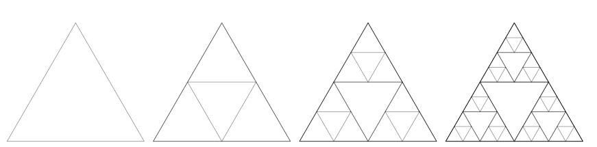
$\ldots\longrightarrow$

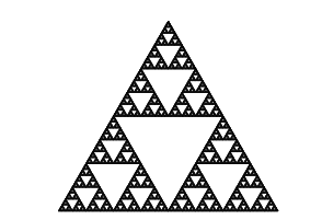
Figure 2. The Sierpiński gasket is a limit of graphs in the plane for the Hausdorff distance

The Sierpiński gasket is a prototype fractal, and has been extensively studied. In [6], a spectral triple was constructed on the Sierpiński gasket. Since the Sierpiński gasket is, naturally, the limit of the graphs $\mathcal{SG}_{n}$ as $n$ goes to $\infty$, a natural question is whether the spectral triple of [6] is the limit of spectral triples on $\mathcal{SG}_{n}$ as $n$ varies in ${\mathds{N}}$.

We answered this question positively in [23], using the metric defined in the present paper. We briefly recall the construction of the spectral triples involved, which are constructed using direct sums of spectral triples over the unit interval, appropriately re-scaled.

Let $\mathrm{CP}$ be the unital Abelian C*-algebra of all ${\mathds{C}}$-valued continuous functions $f$ over $[0,1]$ such that $f(0)=f(1)$:

$$\mathrm{CP}=\left\{f\in C([-1,1]):f(-1)=f(1)\right\}\text{.}$$

The Gelfand spectrum of $\mathrm{CP}$ is of course homeomorphic to the unit circle ${\mathds{T}}=\{z\in{\mathds{C}}:|z|=1\}$ in ${\mathds{R}}^{2}$.

We now define a spectral triple on $\mathrm{CP}$. Let $\mathscr{J}$ be the Hilbert space closure of $\mathrm{CP}$ for the inner product $(f,g)\in\mathrm{CP}\mapsto\int_{-1}^{1}fg$. As usual, we identify $f\in\mathrm{CP}$ with the multiplication operator by $f$ on $\mathscr{J}$.

For each $k\in{\mathds{Z}}$, let $e_{k}:t\in[-1,1]\mapsto\exp(i\pi kt)$ — of course, $e_{k}\in\mathscr{J}$. We define $D$ as the closure of the linear extension of the map defined as:

$$\forall k\in{\mathds{Z}}\quad De_{k}=\pi\left(k+\frac{1}{2}\right)e_{k}\text{.}$$

A standard argument establishes that, indeed, $\left(\mathrm{CP},\mathscr{J},D\right)$ is a spectral triple over $\mathrm{CP}$ [6]. Moreover, the Connes metric induced by this spectral triple on ${\mathds{T}}$, seen as the Gelfand spectrum of $\mathrm{CP}$, is the usual geodesic distance of ${\mathds{T}}$ (i.e. the distance between two points is the smallest of the lengths of the two arcs between these points).

We now use the spectral triple $(\mathrm{CP},\mathscr{J},D)$ in order to construct a spectral triple on the unit interval $[0,1]$. If $f\in C([0,1])$, then the map $t\in[-1,1]\mapsto f(|t|)$ is in $CP$. Let $\varpi$ be the faithful *-representation of $C([0,1])$ on $\mathscr{J}$ defined by

$$\forall f\in C([0,1]),\quad\forall\xi\in\mathscr{J},\quad\varpi(f)\xi:t\in[-1,1]\mapsto f(|t|)\xi(t)\text{.}$$

It is easy to check that $\left(C([0,1]),\mathscr{J},D\right)$ is a metric spectral triple over $C([0,1])$ which induces the usual metric on $[0,1]$.

We now construct our spectral triple over $\mathcal{SG}_{n}$ for all $n\in{\mathds{N}}\cup\{\infty\}$. Let $n\in{\mathds{N}}$ and $j\in\{1,\ldots,3^{n}\}$ be given. Let $w_{0},w_{1},w_{2}\in V_{n}$ be the vertices of the triangle $\Delta_{n,j}$ listed in counter-clockwise order. We parametrize $\Delta_{n,j}$ by defining the following map:

$$r_{n,j}:t\in\left[0,1\right]\longmapsto\begin{cases}(1-3t)w_{0}+3tw_{1}\text{ if $3t\in[0,1]$,}\\ (2-3t)w_{1}+(3t-1)w_{2}\text{ if $3t\in[1,2]$,}\\ (3-3t)w_{2}+(3t-2)w_{0}\text{ if $3t\in[2,3]$.}\end{cases}$$

We can define a spectral triple $\left(C(\Delta_{n,j}),\pi_{n,j},\frac{2^{n}}{3}D\right)$ where $\pi_{n,j}$ is the representation of $C(\Delta_{n,j})$ on $\mathscr{J}$ which sends $f\in C(\Delta_{n,j})$ to the multiplication operator by $f\circ r_{n,j}\in\mathrm{CP}$ on $\mathscr{J}$. It is now easy to check that in particular, $\Delta_{n,j}$ with the induced Monge-Kantorovich metric is isometric to $\Delta_{n,j}$ with the geodesic distance induced on $\Delta_{n,j}$ by the Euclidean metric ${\mathds{R}}^{2}$.

Now, let $n\in{\mathds{N}}\cup\{\infty\}$ and write ${\mathscr{H}}_{n}=\oplus_{k=1}^{n}\oplus_{j=0}^{3^{k}}\mathscr{J}$. For each $k\in{\mathds{N}}$ with $k\leqslant n$ and for all $j\in\{1,\ldots,3^{n}\}$, we define $q_{k,j}:C(\mathcal{SG}_{n})\twoheadrightarrow C(\Delta_{k,j})$ as the quotient map which restricts a function in $C(\mathcal{SG}_{n})$ to $\Delta_{k,j}\subseteq\mathcal{SG}_{n}$. We now define a representation of $C(\mathcal{SG}_{n})$ on ${\mathscr{H}}_{n}$ as the diagonal representation by setting for all $f\in C(\mathcal{SG}_{n})$ and $\xi=(\xi_{k,j})_{k\in{\mathds{N}}_{n},j\in\{1,\ldots,3^{k}\}}$:

$$\pi_{n}(f)\xi=\left(\pi_{k,j}(q_{k,j}(f))\xi_{k,j}\right)_{k\in{\mathds{N}}_{n},j\in\{1,\ldots,3^{k}\}}\text{.}$$

Last, for all $\xi=(\xi_{k,j})_{k\in{\mathds{N}}_{n},j\in\{1,\ldots,3^{k}\}}\in{\mathscr{H}}_{n}$, we set:

$$D_{n}\xi=\left(\frac{2^{k}}{3}D\xi_{k,j}\right)_{k\in{\mathds{N}}_{n},j\in\{1,\ldots,3^{k}\}}\text{.}$$

For all $n\in{\mathds{N}}\cup\{\infty\}$, the triple $\left(C(\mathcal{SG}_{n}),{\mathscr{H}}_{n},D_{n}\right)$ is a metric spectral triple, as seen in [6]. Moreover, the Connes metric induced on $C(\mathcal{SG}_{n})$ by $\left(C(\mathcal{SG}_{n}),{\mathscr{H}}_{n},D_{n}\right)$ is the geodesic distance on $\mathcal{SG}_{n}$ (not the restriction of the metric from ${\mathds{R}}^{2}$).

We prove in [23]:

Theorem 5.1.

The following limit holds:

$$\lim_{n\rightarrow\infty}{\mathsf{\Lambda}^{\mathsf{spec}}_{{F},{F}_{\mathsf{inner}},{F}_{\mathsf{mod}}}}\left(\left(C(\mathcal{SG}_{n}),{\mathscr{H}}_{n},D_{n}\right),\left(C(\mathcal{SG}_{\infty}),{\mathscr{H}}_{\infty},D_{\infty}\right)\right)=0\text{.}$$

In [23], Theorem (5.1) is actually established for a larger class of fractals, called piecewise $C^{1}$ fractal curves, which include the Sierpiński gasket, as well as its Harmonic cousin, called the Harmonic gasket, thus providing a long list of interesting examples of convergence of spectral triples, from the noncommutative geometric study of fractals.

5.3. Approximation of Some Spectral Triples on Quantum Tori

A common example of a finite dimensional, quantum space used in mathematical physics as an approximation of the $2$-torus ${\mathds{T}}^{2}$, where ${\mathds{T}}=\{z\in{\mathds{C}}:|z|=1\}$ is the C*-algebra generated by the so-called clock-and-shift matrices:

(5.4) $$S_{n}=\pNiceMatrix 0&10\Cdots 0\\ \Vdots\Ddots\Ddots\Ddots\Vdots\\ 0\\ 0\Cdots 01\\ 10\Cdots 0\text{ and }C_{n}=\pNiceMatrix 1&\\ \exp\left(\frac{2i\pi}{n}\right)\\ \Ddots\\ \exp\left(\frac{2i(n-1)\pi}{n}\right)\text{,}$$

Such approximations are discussed informally in various contexts, from quantum mechanics in finite dimension [54] to matrix models in quantum field theory and string theory [22, 51, 4, 10, 52]. A first formalization of this heuristics was given in [26], where we proved that there indeed exist quantum metrics on $C^{\ast}(C_{n},S_{n})$ such that the sequence $(C^{\ast}(C_{n},S_{n}))_{n\in{\mathds{N}}}$ converges, in the sense of the propinquity, to $C({\mathds{T}}^{2})$, when ${\mathds{T}}^{2}$ is endowed with its usual geodesic metric as a subspace of ${\mathds{R}}^{2}$.

The C*-algebra $C^{\ast}(C_{n},S_{n})$ is *-isomorphic to the C*-algebra of $n\times n$ matrices. A mean to define a geometry on $C^{\ast}(C_{n},S_{n})$ is to define over it a spectral triple. We wish to show that spectral triple on $C^{\ast}(C_{n},S_{n})$ converges to a natural spectral triple on $C({\mathds{T}}^{2})$ for the spectral propinquity. We describe our construction in [40] here for this special case.

The C*-algebra $C({\mathds{T}}^{2})$ is the universal C*-algebra generated by two commuting unitaries; for instance, we can set $U:(z_{1},z_{2})\in{\mathds{T}}^{2}\mapsto z_{1}$ and $V:(z_{1},z_{2})\in{\mathds{T}}^{2}\mapsto z_{2}$ and note that $C({\mathds{T}}^{2})=C^{\ast}(U,V)$. We define a unique, faithful *-representation of $C({\mathds{T}}^{2})$ on ${\mathscr{H}}_{\infty}=\ell^{2}({\mathds{Z}}^{2})$ by setting, for all $\xi\in\ell^{2}({\mathds{Z}}^{2})$:

$$\pi_{\infty}(U)\xi:(m_{1},m_{2})\in{\mathds{Z}}^{2}\mapsto\xi(m_{1}-1,m_{2})\\ \text{ and }\pi_{\infty}(V)\xi:(m_{1},m_{2})\in{\mathds{Z}}^{2}\mapsto\xi(m_{1},m_{2}-1)\text{.}$$

Let $\mathrm{dom}=\left\{\xi\in\ell^{2}({\mathds{Z}}^{2}):\left((|m_{1}|+|m_{2}|)\xi(m_{1},m_{2})\right)\in\ell^{2}({\mathds{Z}}^{2})\right\}$. We also define, for all $\xi\in\mathrm{dom}$:

$$\partial_{U}\xi:(m_{1},m_{2})\in{\mathds{Z}}^{d}\mapsto im_{1}\xi(m_{1},m_{2})\\ \text{ and }\partial_{V}\xi:(m_{1},m_{2})\in{\mathds{Z}}^{d}\mapsto im_{2}\xi(m_{1},m_{2})\text{.}$$

The canonical moving frame of the compact Lie group ${\mathds{T}}^{2}$ is given by $[\partial_{U},\pi_{\infty}(\cdot)]$ and $[\partial_{V},\pi_{\infty}(\cdot)]$.

Fix $n\in{\mathds{N}}\setminus\{0\}$. The C*-algebra $C^{\ast}(C_{n},S_{n})$ is the universal C*-algebra generated by two unitaries whose multiplicative commutator is $\zeta_{n}=\exp\left(\frac{2i\pi}{n}\right)$, and it is *-isomorphic to the C*-algebra ${\mathfrak{M}}_{n}$ of $n\times n$ matrices. Let ${\mathscr{H}}_{n}$ be the Hilbert space obtained by endowing ${\mathfrak{M}}_{n}=C^{\ast}(C_{n},S_{n})$ with the usual inner product $(a,b)\in{\mathfrak{M}}_{n}\mapsto{\left<{a},{b}\right>_{n}}\coloneqq\mathrm{trace}(a^{\ast}b)$, with $\mathrm{trace}$ the usual normalized trace over ${\mathfrak{M}}_{n}$. As $C^{\ast}(C_{n},S_{n})$ is finite dimensional, it is complete for the Hilbert norm associated with ${\left<{\cdot},{\cdot}\right>_{n}}$. Note that $C^{\ast}(C_{n},S_{n})$ acts on ${\mathscr{H}}_{n}$ canonically on both the left and the right, in such a way that ${\mathscr{H}}_{n}$ is a bimodule over $C^{\ast}(C_{n},S_{n})$.

As explained, for instance, in [22, 51, 4], natural substitutes for the derivations $\partial_{U}$ and $\partial_{V}$, when working with fuzzy tori, is given by the commutators:

$$\frac{n}{2\pi}[C_{n},\cdot]\text{ and }\frac{n}{2\pi}[S_{n}^{\ast},\cdot]$$

seen as operators on ${\mathscr{H}}_{n}$. However, we will want to work with skew-adjoint operators in order to define a Dirac operator. With this in mind, we are able to prove the following convergence result.

Theorem 5.2 ([40]).

We use the notations developed in this subsection.

Let $\gamma_{1},\gamma_{2},\gamma_{3},\gamma_{4}$ be $4\times 4$ matrices such that

$$\forall j,s\in\{1,\ldots,4\}\quad\gamma_{j}\gamma_{s}+\gamma_{s}\gamma_{j}=\begin{cases}-2\text{ if $j=s$,}\\ 0\text{ otherwise.}\end{cases}$$

For all $n\in{\mathds{N}}$, we define the operator $D_{n}$ on $\ell^{2}(H_{n})\otimes{\mathds{C}}^{4}$, by

$$D_{n}=\frac{n}{2\pi}\bigg{(}\left[\frac{C_{n}+C_{n}^{\ast}}{2},\cdot\right]\otimes\gamma_{1}+\left[\frac{C_{n}-C_{n}^{\ast}}{2i},\cdot\right]\otimes\gamma_{2}\\ +\left[\frac{S_{n}+S_{n}^{\ast}}{2},\cdot\right]\otimes\gamma_{3}+\left[\frac{S_{n}^{\ast}-S_{n}}{2i},\cdot\right]\otimes\gamma_{4}\bigg{)}\text{.}$$

We also define the operator $D_{\infty}$ from $\mathrm{dom}\otimes{\mathds{C}}^{4}$ to $\ell^{2}({\mathds{Z}}^{2})\otimes{\mathds{C}}^{4}$ by setting:

$$D_{\infty}=\pi_{\infty}\left(\frac{U+U^{\ast}}{2}\right)\partial_{V}\otimes\gamma_{1}+\pi_{\infty}\left(\frac{U-U^{\ast}}{2}\right)\partial_{V}\otimes\gamma_{2}\\ +\pi_{\infty}\left(\frac{V+V^{\ast}}{2}\right)\partial_{U}\otimes\gamma_{3}+\pi_{\infty}\left(\frac{V^{\ast}-V}{2}\right)\partial_{U}\otimes\gamma_{4}\text{.}$$

For each $n\in{\mathds{N}}\cup\{\infty\}$, the triple $({\mathfrak{A}}_{n},\mathscr{J}_{n},D_{n})$ is a metric spectral triple over ${\mathfrak{A}}_{n}$, and moreover:

$$\lim_{n\rightarrow\infty}{\mathsf{\Lambda}^{\mathsf{spec}}_{{5},{5}_{\mathsf{inner}},{5}_{\mathsf{mod}}}}(({\mathfrak{A}}_{n},\mathscr{J}_{n},D_{n}),({\mathfrak{A}}_{\infty},\mathscr{J}_{\infty},D_{\infty}))=0\text{,}$$

where ${\mathsf{\Lambda}^{\mathsf{spec}}_{{5},{5}_{\mathsf{inner}},{5}_{\mathsf{mod}}}}$ is the spectral propinquity for the admissible triple $(F,F_{\mathsf{inner}},F_{\mathsf{mod}})$, with

$$F:x,y,l_{x},l_{y}\in{\mathds{R}}_{+}\mapsto xl_{y}+yl_{x}\text{, }G:x,y,z\in{\mathds{R}}_{+}\mapsto 5(x+y)z\\ \text{ and }H:x,y\in{\mathds{R}}_{+}\mapsto 2x^{2}y^{2}\text{.}$$

Remark 5.3.

We note that we relax a little bit the Leibniz condition for the previous result, to accommodate some of the tunnels constructed in [40].

In fact, the above construction can be generalized to noncommutative limits. In general, we require the introduction of certain auxiliary unitaries to construct our spectral triples over quantum tori, so the description is more involved. We establish in [40] that, for any quantum torus, there exists a natural spectral triple, constructed from the dual action of the torus, which is the limit of spectral triples on fuzzy tori, with the obvious requirement on the twist of the fuzzy tori (coded in a $2$-cocycle) to converge to the twist of the quantum torus (similarly coded).

References

• [1] K. Aguilar and J. Kaad, The podleś sphere as a spectral metric space., J. Geom. Phys. 133 (2018), 260–278.
• [2] K. Aguilar and F. Latrémolière, Quantum ultrametrics on AF algebras and the Gromov–Hausdorff propinquity, Studia Math. 231 (2015), no. 2, 149–194, ArXiv: 1511.07114.
• [3] by same author, Some applications of conditional expectations to convergence for the Gromov-Hausdorff propinquity, Banach Center Publ. 120 (2021), 35–46, arXiv:1708.00595.
• [4] J. Barrett, Matrix geometries and fuzzy spaces as finite spectral triples, J. Math. Phys. 56 (2015), no. 8, 082301, 25pp.
• [5] E. Christensen, Higher weak derivatives and reflexive algebras of operators, Operator algebras and their applications, Contemp. Math., no. 671, Amer. Math. Soc., Providence, RI, 2016, arXiv:1504.03521, p. 69–83.
• [6] E. Christensen, C. Ivan, and M. Lapidus, Dirac operators and spectral triples for some fractal sets built on curves, Adv. Math. 217 (2008), no. 1, 42–78.
• [7] A. Connes, C*–algèbres et géométrie differentielle, C. R. de l’Academie des Sciences de Paris (1980), no. series A-B, 290.
• [8] A. Connes, Compact metric spaces, Fredholm modules and hyperfiniteness, Ergodic Theory Dynam. Systems 9 (1989), no. 2, 207–220.
• [9] by same author, Noncommutative geometry, Academic Press, San Diego, 1994.
• [10] A. Connes, M. Douglas, and A. Schwarz, Noncommutative geometry and matrix theory: Compactification on tori, JHEP 9802 (1998), hep-th/9711162.
• [11] Francesco D’Andrea, Fedele Lizzi, and Pierre Martinetti, Spectral geometry with a cut-off: topological and metric aspects, J. Geom. Phys. 82 (2014), 18–45, arXiv: 1305.2605. MR 3206638
• [12] S. Doplicher, K. Fredenhagen, and J. E. Roberts, The quantum structure of spacetime at the plank scale and quantum fields, Comm. Math. Phys. 172 (1995), 187–220.
• [13] David A. Edwards, The structure of superspace, Studies in topology (Proc. Conf., Univ. North Carolina, Charlotte, N. C., 1974; dedicated to Math. Sect. Polish Acad. Sci.), 1975, p. 121–133. MR 0401069
• [14] Nicolas Franco and Jean-Christophe Wallet, Metrics and causality on Moyal planes, Noncommutative geometry and optimal transport, Contemp. Math., vol. 676, Amer. Math. Soc., Providence, RI, 2016, arXiv: 1507.06559, p. 147–173. MR 3578739
• [15] M. Gromov, Groups of polynomial growth and expanding maps, Publ. Math. Inst. Hautes Études Sci. 53 (1981), 53–78.
• [16] by same author, Metric structures for Riemannian and non-Riemannian spaces, Progress in Mathematics, Birkhäuser, 1999.
• [17] F. Hausdorff, Grundzüge der Mengenlehre, Verlag Von Veit und Comp., 1914.
• [18] A. O. Ivanov, N. K. Nikolaeva, and A. A. Tuzhilin, The gromov-hausdorff metric on the space of compact metric spaces is strictly intrinsic, Mat. Zametki 100 (2016), no. 6, 947–950, translation in Math. Notes 100 (2016), no. 5-6, 883–885.
• [19] J. Kaad, Differentiable absorption of Hilbert $C^{*}$-modules, connections, and lifts of unbounded operators, J. Noncommut. Geom. 11 (2017), no. 3, 1037–1068, arXiv:1407.1389.
• [20] J. Kaad and M. Lesch, Spectral flow and the unbounded Kasparov product, Adv. Math. 248 (2013), 495–530.
• [21] T. Kato, Perturbation theory for linear operators, Springer, 1995.
• [22] Y. Kimura, Noncommutative gauge theories on fuzzy sphere and fuzzy torus from matrix model, Nuclear Phys. B 604 (2001), no. 1–2, 121–147.
• [23] T. Landry, M. Lapidus, and F. Latrémolière, Metric approximations of the spectral triple on the Sierpinki gasket and other fractals, Adv. Math. 385 (2021), Paper No. 107771, 43 pp.
• [24] F. Latrémolière, Approximation of the quantum tori by finite quantum tori for the quantum Gromov-Hausdorff distance, J. Funct. Anal. 223 (2005), 365–395, math.OA/0310214.
• [25] by same author, Quantum locally compact metric spaces, J. of Funct. Anal. 264 (2013), no. 1, 362–402, arXiv: 1208.2398.
• [26] by same author, Convergence of fuzzy tori and quantum tori for the quantum Gromov–Hausdorff propinquity: an explicit approach., Münster J. Math. 8 (2015), no. 1, 57–98, arXiv: math/1312.0069.
• [27] by same author, Curved noncommutative tori as Leibniz compact quantum metric spaces, J. Math. Phys. 56 (2015), no. 12, 123503, 16 pages, arXiv: 1507.08771.
• [28] by same author, The dual Gromov–Hausdorff propinquity, J. Math. Pures Appl. 103 (2015), no. 2, 303–351, arXiv: 1311.0104.
• [29] by same author, Quantum metric spaces and the Gromov-Hausdorff propinquity, Noncommutative geometry and optimal transport, Contemp. Math., no. 676, Amer. Math. Soc., 2015, arXiv: 150604341, p. 47–133.
• [30] by same author, Equivalence of quantum metrics with a common domain, J. Math. Anal. Appl. 443 (2016), 1179–1195, arXiv: 1604.00755.
• [31] by same author, The quantum Gromov-Hausdorff propinquity, Trans. Amer. Math. Soc. 368 (2016), no. 1, 365–411.
• [32] by same author, A compactness theorem for the dual Gromov-Hausdorff propinquity, Indiana Univ. Math. J. 66 (2017), no. 5, 1707–1753, arXiv: 1501.06121.
• [33] by same author, The triangle inequality and the dual Gromov-Hausdorff propinquity, Indiana Univ. Math. J. 66 (2017), no. 1, 297–313, arXiv: 1404.6633.
• [34] by same author, Actions of categories by Lipschitz morphisms on limits for the Gromov-Hausdorff propinquity, J. Geom. Phys. 146 (2019), 103481, 31 pp., arXiv: 1708.01973.
• [35] by same author, Convergence of Cauchy sequences for the covariant Gromov-Hausdorff propinquity, J. Math. Anal. Appl. 469 (2019), no. 1, 378–404, arXiv: 1806.04721.
• [36] by same author, The modular Gromov–Hausdorff propinquity, Dissertationes Math. 544 (2019), 1–70, arXiv: 1608.04881.
• [37] by same author, Convergence of Heisenberg modules for the modular Gromov-Hausdorff propinquity, J. Operator Theory 84 (2020), no. 1, 211–237.
• [38] by same author, The covariant Gromov-Hausdorff propinquity, Studia Math. 251 (2020), no. 2, 135–169, arXiv: 1805.11229.
• [39] by same author, Heisenberg modules over quantum $2$-tori are metrized quantum vector bundles, Canad. J. Math 72 (2020), no. 4, 1044–1081, arXiv: 1703.07073.
• [40] by same author, Convergence of spectral triples on fuzzy tori to spectral triples on quantum tori, Comm. Math. Phys. 388 (2021), no. 2, 1049–1128, arXiv: 2102.03729.
• [41] by same author, The dual-modular Gromov-Hausdorff propinquity and completeness, J. Noncomm. Geometry 115 (2021), no. 1, 347–398.
• [42] F. Latrémolière and J. Packer, Noncommutative solenoids and the Gromov-Hausdorff propinquity, Proc. Amer. Math. Soc. 145 (2017), no. 5, 1179–1195, arXiv: 1601.02707.
• [43] E. J. McShane, Extension of range of functions, Bull. Amer. Math. Soc. 40 (1934), no. 12, 825–920.
• [44] B. Mesland, Unbounded bivariant $K$-theory and correspondences in noncommutative geometry, J. Reine Angew. Math. 691 (2014), 101–172, arXiv:0904.4383.
• [45] M. A. Rieffel, Deformation-quantization for actions of ${\mathds{R}}^{d}$, Memoirs of the AMS, vol. 106, American Mathematical Society, 1993.
• [46] M. A. Rieffel, Metrics on states from actions of compact groups, Doc. Math. 3 (1998), 215–229, math.OA/9807084.
• [47] by same author, Metrics on state spaces, Doc. Math. 4 (1999), 559–600, math.OA/9906151.
• [48] by same author, Gromov-Hausdorff distance for quantum metric spaces, Mem. Amer. Math. Soc. 168 (2004), no. 796, 1–65, math.OA/0011063.
• [49] by same author, Leibniz seminorms for "matrix algebras converge to the sphere", Clay Mathematics Proceedings 11 (2010), 543–578, arXiv: 0707.3229.
• [50] Marc A. Rieffel, Matricial bridges for “matrix algebras converge to the sphere”, Operator algebras and their applications, Contemp. Math., vol. 671, Amer. Math. Soc., Providence, RI, 2016, arXiv: 1502.00329, p. 209–233. MR 3546687
• [51] P. Schreivogl and H. Steinacker, Generalized fuzzy torus and its modular properties, SIGMA 9 (2013), no. 060, 23 pages.
• [52] N. Seiberg and E. Witten, String theory and noncommutative geometry, JHEP 9909 (1999), no. 32, arXiv: hep-th/9908142.
• [53] J. Wallet, Connes distance by examples: Homothetic spectral metric spaces, Rev. Math. Phys. 24 (2012), no. 9, arXiv: 1112.3285.
• [54] H. Weyl, The theory of groups and quantum mechanics, Dover Publication, N.Y., 1950, Translated from the second (revised) German edition by H. P. Robertson.
• [55] J. Wheeler, Superspace and the nature of quantum geometrodynamics, Battelle Rencontres. 1967 Lectures in Mathematics and Physics (DeWitt C. and J. Wheeler, eds.), 1968.