A Frank-Wolfe Framework for Efficient and Effective Adversarial Attacks

Abstract

Depending on how much information an adversary can access to, adversarial attacks can be classified as white-box attack and black-box attack. For white-box attack, optimization-based attack algorithms such as projected gradient descent (PGD) can achieve relatively high attack success rates within moderate iterates. However, they tend to generate adversarial examples near or upon the boundary of the perturbation set, resulting in large distortion. Furthermore, their corresponding black-box attack algorithms also suffer from high query complexities, thereby limiting their practical usefulness. In this paper, we focus on the problem of developing efficient and effective optimization-based adversarial attack algorithms. In particular, we propose a novel adversarial attack framework for both white-box and black-box settings based on a variant of Frank-Wolfe algorithm. We show in theory that the proposed attack algorithms are efficient with an $O(1/\sqrt{T})$ convergence rate. The empirical results of attacking the ImageNet and MNIST datasets also verify the efficiency and effectiveness of the proposed algorithms. More specifically, our proposed algorithms attain the best attack performances in both white-box and black-box attacks among all baselines, and are more time and query efficient than the state-of-the-art.

1 Introduction

Deep Neural Networks (DNNs) have made many breakthroughs in different areas of artificial intelligence such as image classification (Krizhevsky et al., 2012; He et al., 2016), object detection (Ren et al., 2015; Girshick, 2015), and speech recognition (Mohamed et al., 2012; Bahdanau et al., 2016). However, recent studies show that deep neural networks are vulnerable to adversarial examples (Szegedy et al., 2013; Goodfellow et al., 2015) – a tiny perturbation on an image that is almost invisible to human eyes could mislead a well-trained image classifier towards misclassification. Soon later this is proved to be not a coincidence in image classification: similar phenomena have been observed in other problems such as speech recognition (Carlini et al., 2016), visual QA (Xu et al., 2017), image captioning (Chen et al., 2017a), machine translation (Cheng et al., 2018), reinforcement learning (Pattanaik et al., 2018), and even on systems that operate in the physical world (Kurakin et al., 2016).

Depending on how much information an adversary can access to, adversarial attacks can be classified into two classes: white-box attack (Szegedy et al., 2013; Goodfellow et al., 2015) and black-box attack (Papernot et al., 2016a; Chen et al., 2017c). In the white-box setting, the adversary has full access to the target model, while in the black-box setting, the adversary can only access the input and output of the target model but not its internal configurations.

Several optimization-based methods have been proposed for the white-box attack. One of the first successful attempt is the FGSM method (Goodfellow et al., 2015), which works by linearizing the network loss function. CW method (Carlini and Wagner, 2017) further improves the attack effectiveness by designing a regularized loss function based on the logit-layer output of the network and optimizing the loss by Adam (Kingma and Ba, 2015). Even though CW largely improves the effectiveness, it requires a large number of gradient iterations to optimize the distortion of the adversarial examples. Iterative gradient (steepest) descent based methods such as PGD (Madry et al., 2018) and I-FGSM (Kurakin et al., 2016) can achieve relatively high attack success rates within a moderate number of iterations. However, they tend to generate adversarial examples near or upon the boundary of the perturbation set, due to the projection nature of the algorithm. This leads to large distortion in the resulting adversarial examples.

In the black-box attack, since one needs to make gradient estimations in such setting, a large number of queries are required to perform a successful black-box attack, especially when the data dimension is high. A naive way to estimate gradient direction is to perform finite difference approximation on each dimension (Chen et al., 2017c). This would take $O(d)$ queries to performance one full gradient estimation where $d$ is the data dimension and therefore result in inefficient attacks. For example, attacking a $299\times 299\times 3$ ImageNet (Deng et al., 2009) image may take hundreds of thousands of queries. This significantly limits the practical usefulness of such algorithms since they can be easily defeated by limiting the number of queries that an adversary can make to the target model. Although recent studies (Ilyas et al., 2018a, b) have improved the query complexity by using Gaussian sensing vectors or gradient priors, due to the inefficiencies of PGD framework, there is still room for improvements.

In this paper, we propose efficient and effective optimization-based adversarial attack algorithms based on a variant of Frank-Wolfe algorithm. We show in theory that the proposed attack algorithms are efficient with guaranteed convergence rate. The empirical results also verify the efficiency and effectiveness of our proposed algorithms.

In summary, we make the following main contributions:

1. We develop a new Frank-Wolfe based projection-free attack framework with momentum mechanism. The framework contains an iterative first-order white-box attack algorithm which admits the fast gradient sign method (FGSM) as a one-step special case, and also a corresponding black-box attack algorithm which adopts zeroth-order optimization with two sensing vector options (either from the Euclidean unit sphere or from the standard Gaussian distribution).

2. We prove that the proposed white-box and black-box attack algorithms with momentum mechanism enjoy an $O(1/\sqrt{T})$ convergence rate in the nonconvex setting. We also show that the query complexity of the proposed black-box attack algorithm is linear in data dimension $d$.

3. Our experiments on MNIST and ImageNet datasets show that (i) the proposed white-box attack algorithm has better distortion and is more efficient than all the state-of-the-art white-box attack baseline algorithms, and (ii) the proposed black-box attack algorithm is highly query efficient and achieves the highest attack success rate among other baselines.

The remainder of this paper is organized as follows: in Section 2, we briefly review existing literature on adversarial examples and Frank-Wolfe algorithm. We present our proposed Frank-Wolfe framework in Section 3, and the main theory in Section 4. In Section 5, we compare the proposed algorithms with state-of-the-art adversarial attack algorithms on ImageNet and MNIST datasets. Finally, we conclude this paper in Section 6.

2 Related Work

There is a large body of work on adversarial attacks. In this section, we review the most relevant work in both white-box and black-box attack settings, as well as the non-convex Frank-Wolfe optimization.

White-box Attacks: Szegedy et al. (2013) proposed to use box-constrained L-BFGS algorithm for conducting white-box attacks. Goodfellow et al. (2015) proposed the Fast Gradient Sign Method (FGSM) based on linearization of the network as a simple alternative to L-BFGS. Kurakin et al. (2016) proposed to iteratively perform one-step FGSM (Goodfellow et al., 2015) algorithm and clips the adversarial point back to the distortion limit after every iteration. It is called Basic Iterative Method (BIM) or I-FGM in the literature. Madry et al. (2018) showed that for the $L_{\infty}$ norm case, BIM/I-FGM is almost equivalent to Projected Gradient Descent (PGD), which is a standard tool for constrained optimization. Papernot et al. (2016b) proposed JSMA to greedily attack the most significant pixel based on the Jacobian-based saliency map. Moosavi-Dezfooli et al. (2016) proposed attack methods by projecting the data to the closest separating hyperplane. Carlini and Wagner (2017) introduced the so-called CW attack by proposing multiple new loss functions for generating adversarial examples. Chen et al. (2017b) followed CW’s framework and use an Elastic Net term as the distortion penalty. Dong et al. (2018) proposed MI-FGSM to boost the attack performances using momentum.

Black-box Attacks: One popular family of black-box attacks (Hu and Tan, 2017; Papernot et al., 2016a, 2017) is based on the transferability of adversarial examples (Liu et al., 2018; Bhagoji et al., 2017), where an adversarial example generated for one DNN may be reused to attack other neural networks. This allows the adversary to construct a substitute model that mimics the targeted DNN, and then attack the constructed substitute model using white-box attack methods. However, this type of attack algorithms usually suffer from large distortions and relatively low success rates (Chen et al., 2017c). To address this issue, Chen et al. (2017c) proposed the Zeroth-Order Optimization (ZOO) algorithm that extends the CW attack to the black-box setting and uses a zeroth-order optimization approach to conduct the attack. Although ZOO achieves much higher attack success rates than the substitute model-based black-box attacks, it suffers from a poor query complexity since its naive implementation requires to estimate the gradients of all the coordinates (pixels) of the image. To improve its query complexity, several approaches have been proposed. For example, Tu et al. (2018) introduces an adaptive random gradient estimation algorithm and a well-trained Autoencoder to speed up the attack process. Ilyas et al. (2018a) and Liu et al. (2018) improved ZOO’s query complexity by using Natural Evolutionary Strategies (NES) (Wierstra et al., 2014; Salimans et al., 2017) and active learning, respectively. Ilyas et al. (2018b) further improve the performance by considering the gradient priors.

Non-convex Frank-Wolfe Algorithms: The Frank-Wolfe algorithm (Frank and Wolfe, 1956), also known as the conditional gradient method, is an iterative optimization method for constrained optimization problem. Jaggi (2013) revisited Frank-Wolfe algorithm in 2013 and provided a stronger and more general convergence analysis in the convex setting. Yu et al. (2017) proved the first convergence rate for Frank-Wolfe type algorithm in the non-convex setting. Lacoste-Julien (2016) provided the convergence guarantee for Frank-Wolfe algorithm in the non-convex setting with adaptive step sizes. Reddi et al. (2016) further studied the convergence rate of non-convex stochastic Frank-Wolfe algorithm in the finite-sum optimization setting. Very recently, Staib and Jegelka (2017) proposed to use Frank-Wolfe for distributionally robust training (Sinha et al., 2018). Balasubramanian and Ghadimi (2018) proved the convergence rate for zeroth-order nonconvex Frank-Wolfe algorithm using one-side finite difference gradient estimator with standard Gaussian sensing vectors.

3 Methodology

3.1 Notation

Throughout the paper, scalars are denoted by lower case letters, vectors by lower case bold face letters and sets by calligraphy upper cae letters. For a vector $\mathbf{x}\in\mathbb{R}^{d}$, we denote the $L_{p}$ norm of $\mathbf{x}$ by $\|\mathbf{x}\|_{p}=(\sum_{i=1}^{d}x_{i}^{p})^{1/p}$. Specially, for $p=\infty$, the $L_{\infty}$ norm of $\mathbf{x}$ by $\|\mathbf{x}\|_{\infty}=\max_{i=1}^{d}|\theta_{i}|$. We denote $\mathcal{P}_{\mathcal{X}}(\mathbf{x})$ as the projection operation of projecting vector $\mathbf{x}$ into the set $\mathcal{X}$.

3.2 Problem Formulation

According to the attack purposes, attacks can be divided into two categories: untargeted attack and targeted attack.

In particular, untargeted attack aims to turn the prediction into any incorrect label, while the targeted attack, requires to mislead the classifier to a specific target class. In this work, we focus on the strictly harder targeted attack setting (Carlini and Wagner, 2017; Ilyas et al., 2018a). It is worth noting that our proposed algorithm can be extended to untargeted attack straightforwardly. To be more specific, let us define $\ell(\mathbf{x},y)$ as the classification loss function of the targeted DNN with an input $\mathbf{x}\in\mathbb{R}^{d}$ and a corresponding label $y$. For targeted attacks, we aim to minimize $\ell(\mathbf{x},y_{\text{tar}})$ to learn an adversarial example that will be misclassified to the target class $y_{\text{tar}}$. In the rest of this paper, let $f(\mathbf{x})=\ell(\mathbf{x},y_{\text{tar}})$ be the attack loss function for simplicity, and the corresponding targeted attack problem can be formulated as the following optimization problem:

$$\min_{\mathbf{x}} f(\mathbf{x})$$ (3.1)

subject to $$\|\mathbf{x}-\mathbf{x}_{\rm{ori}}\|_{p}\leq\epsilon.$$

Evidently, the constraint set $\mathcal{X}:=\{\mathbf{x}\ |\ \|\mathbf{x}-\mathbf{x}_{\rm{ori}}\|_{p}\leq\epsilon\}$ is a bounded convex set when $p\geq 1$. Note that even though we mainly focus on the most popular $L_{\infty}$ attack case in this paper, our proposed methods can easily extend to general $p\geq 1$ case.

3.3 Frank-Wolfe vs. PGD

Although PGD can achieve relatively high attack success rate within moderate iterates, the multi-step update formula requires an additional projection step at each iteration to keep the iterates within the constraint set. This tends to cause the generated adversarial examples near or upon the boundary of the constraint set, and leads to relatively large distortion. This motivates us to use Frank-Wolfe based optimization algorithm Frank and Wolfe (1956). Different from PGD, Frank-Wolfe algorithm is projection-free as it calls a Linear Minimization Oracle (LMO) over the constraint set $\mathcal{X}$ at each iteration, i.e.,

$${\rm{LMO}}\in\mathop{\mathrm{argmin}}_{\mathbf{x}\in\mathcal{X}}\langle\mathbf{x},\nabla f(\mathbf{x}_{t})\rangle.$$

The LMO can be seen as the minimization of the first-order Taylor expansion of $f(\cdot)$ at point $\mathbf{x}_{t}$:

$$\min_{\mathbf{x}\in\mathcal{X}}f(\mathbf{x}_{t})+\langle\mathbf{x}-\mathbf{x}_{t},\nabla f(\mathbf{x}_{t})\rangle.$$

By calling LMO, Frank Wolfe solves the linear problem in $\mathcal{X}$ and then perform weighted average with previous iterate to obtain the final update formula.

Comparing the two methods, PGD is a more “aggressive” approach. It first takes a step towards the negative gradient direction while ignoring the constraint to get a new point (often outside the constraint set), and then correct the new point by projecting it back into the constraint set. In sharp contrast, Frank-Wolfe is more “conservative” as it always keeps the iterates within the constraint set. Therefore, it avoids projection and can lead to better distortion.

3.4 Frank-Wolfe White-box Attacks

The proposed Frank-Wolfe based white-box attack algorithm is shown in Algorithm 1, which is built upon the classic Frank-Wolfe algorithm. The key difference between Algorithm 1 and the classic Frank-Wolfe algorithm is in Line 4, where an additional momentum term $\mathbf{m}_{t}$ is introduced. The momentum term $\mathbf{m}_{t}$ will help stabilize the LMO direction and leads to empirically accelerated convergence of Algorithm 1.

Algorithm 1 Frank-Wolfe White-box Attack Algorithm

1:  input: number of iterations $T$, step sizes $\{\gamma_{t}\}$;

2:  $\mathbf{x}_{0}=\mathbf{x}_{\rm{ori}},\mathbf{m}_{-1}=\nabla f(\mathbf{x}_{0})$

3:  for $t=0,\ldots,T-1$ do

4:     $\mathbf{m}_{t}=\beta\cdot\mathbf{m}_{t-1}+(1-\beta)\cdot\nabla f(\mathbf{x}_{t})$

5:     $\mathbf{v}_{t}=\mathop{\mathrm{argmin}}_{\mathbf{x}\in\mathcal{X}}\langle\mathbf{x},\mathbf{m}_{t}\rangle$   // LMO

6:     $\mathbf{d}_{t}=\mathbf{v}_{t}-\mathbf{x}_{t}$

7:     $\mathbf{x}_{t+1}=\mathbf{x}_{t}+\gamma_{t}\mathbf{d}_{t}$

8:  end for

9:  output: $\mathbf{x}_{T}$

The LMO solution itself can be expensive to obtain in general. Fortunately, for the constraint set $\mathcal{X}$ defined in (3.1), the corresponding LMO has a closed-form solution. Here we provide the closed-form solution of LMO (Line 5 in Algorithm 1) for $L_{\infty}$ norm case:

$$\mathbf{v}_{t}=-\epsilon\cdot\mathop{\mathrm{sign}}(\mathbf{m}_{t})+\mathbf{x}_{\rm{ori}}.$$

Note that if we write down the full update formula at each iteration in Algorithm 1, it becomes

$$\mathbf{x}_{t+1}=\mathbf{x}_{t}-\gamma_{t}\epsilon\cdot\mathop{\mathrm{sign}}(\mathbf{m}_{t})-\gamma_{t}(\mathbf{x}_{t}-\mathbf{x}_{\rm{ori}}).$$ (3.2)

Intuitively speaking, the term $-\gamma_{t}(\mathbf{x}_{t}-\mathbf{x}_{\rm{ori}})$ enforces $\mathbf{x}_{t}$ to be close to $\mathbf{x}_{\rm{ori}}$ for all $t=1,\ldots,T$, which encourages the adversarial example to have a small distortion. This is the key advantage of Algorithm 1.

Comparison with FGSM: When $T=1$, substituting the above LMO solutions into Algorithm 1 yields the final update of $\mathbf{x}_{1}=\mathbf{x}_{0}-\gamma_{t}\epsilon\cdot\mathop{\mathrm{sign}}(\nabla f(\mathbf{x}_{0}))$, which reduces to FGSM when $\gamma_{t}=1$. Therefore, our proposed Frank-Wolfe white-box attack also includes FGSM as a one-step special instance.

3.5 Frank-Wolfe Black-box Attacks

Next we consider the black-box setting, where we cannot perform back-propagation to calculate the gradient of the loss function anymore. Instead, we can only query the DNN system’s outputs with specific inputs. To clarify, here the output refers to the logit layer’s output (confidence scores for classification), not the final prediction label.

We propose a zeroth-order Frank-Wolfe based algorithm to solve this problem in Algorithm 2. The key difference between our proposed black-box attack and white-box attack is one extra gradient estimation step, which is presented in Line 4 in Algorithm 2. Also, the momentum term $\mathbf{m}_{t}$ is now defined as the exponential average of previous gradient estimations $\{\mathbf{q}_{t}\}_{t=0}^{T-1}$. This will help reduce the variance in zeroth-order gradient estimation and empirically accelerate the convergence of Algorithm 2.

Algorithm 2 Frank-Wolfe Black-box Attack Algorithm

1:  input: number of iterations $T$, step sizes $\{\gamma_{t}\}$, sample size for gradient estimation $b$, sampling parameter $\delta$;

2:  $\mathbf{x}_{0}=\mathbf{x}_{\rm{ori}}$, $\mathbf{m}_{-1}={\rm GRAD\_EST}(\mathbf{x}_{0},b,\delta)$

3:  for $t=0,\ldots,T-1$ do

4:     $\mathbf{q}_{t}={\rm GRAD\_EST}(\mathbf{x}_{t},b,\delta)$   // Alg 3

5:     $\mathbf{m}_{t}=\beta\cdot\mathbf{m}_{t-1}+(1-\beta)\cdot\mathbf{q}_{t}$

6:     $\mathbf{v}_{t}=\mathop{\mathrm{argmin}}_{\mathbf{v}\in\mathcal{X}}\langle\mathbf{v},\mathbf{m}_{t}\rangle$

7:     $\mathbf{d}_{t}=\mathbf{v}_{t}-\mathbf{x}_{t}$

8:     $\mathbf{x}_{t+1}=\mathbf{x}_{t}+\gamma_{t}\mathbf{d}_{t}$

9:  end for

10:  output: $\mathbf{x}_{T}$

As in many other zeroth-order optimization algorithms (Shamir, 2017; Flaxman et al., 2005), Algorithm 3 uses symmetric finite differences to estimate the gradient and therefore, gets rid of the dependence on back-propagation in white-box setting. Different from Chen et al. (2017c), here we do not utilize natural basis as our sensing vectors, instead, we provide two options: one is to use vectors uniformly sampled from Euclidean unit sphere and the other is to use vectors uniformly sampled from standard multivarite Gaussian distribution. This will greatly improve the gradient estimation efficiency comparing to sensing with natural basis as such option will only be able to estimate one coordinate of the gradient vector per query. In practice, both options here provide us competitive experimental results. It is worth noting that NES method (Wierstra et al., 2014) with antithetic sampling (Salimans et al., 2017) used in Ilyas et al. (2018a) yields similar formula as our option II in Algorithm 3.

Algorithm 3 GRAD_EST($\mathbf{x},b,\delta$)

1:  $\mathbf{q}={\bm{0}}$

2:  for $i=1,\ldots,b$ do

3:     option I: Sample $\mathbf{u}_{i}$ uniformly from the Euclidean unit sphere with $\|\mathbf{u}_{i}\|_{2}=1$   $\mathbf{q}=\mathbf{q}+\frac{d}{2\delta b}\big{(}f(\mathbf{x}+\delta\mathbf{u}_{i})-f(\mathbf{x}-\delta\mathbf{u}_{i})\big{)}\mathbf{u}_{i}$

4:     option II: Sample $\mathbf{u}_{i}$ uniformly from the standard Gaussian distribution $N({\bm{0}},\mathbf{I})$   $\mathbf{q}=\mathbf{q}+\frac{1}{2\delta b}\big{(}f(\mathbf{x}+\delta\mathbf{u}_{i})-f(\mathbf{x}-\delta\mathbf{u}_{i})\big{)}\mathbf{u}_{i}$

5:  end for

6:  return $\mathbf{q}$

4 Main Theory

In this section, we establish the convergence guarantees for our proposed Frank-Wolfe adversarial attack algorithms described in Section 3. The omitted proofs can be found in the Appendix B. First, we introduce the convergence criterion for our Frank-Wolfe adversarial attack framework.

4.1 Convergence Criterion

The loss function for common DNN models are generally nonconvex. In addition, (3.1) is a constrained optimization. For such general nonconvex constrained optimization, we typically adopt the Frank-Wolfe gap as the convergence criterion (since gradient norm of $f$ is no longer a proper criterion for constrained optimization problems):

$$g(\mathbf{x}_{t})=\max_{\mathbf{x}\in\mathcal{X}}\langle\mathbf{x}-\mathbf{x}_{t},-\nabla f(\mathbf{x}_{t})\rangle.$$

Note that we always have $g(\mathbf{x}_{t})\geq 0$ and $\mathbf{x}_{t}$ is a stationary point for the constrained optimization problem if and only if $g(\mathbf{x}_{t})=0$, which makes $g(\mathbf{x}_{t})$ a perfect convergence criterion for Frank-Wolfe based algorithms.

4.2 Convergence Guarantee for Frank-Wolfe White-box Attack

Before we are going to provide the convergence guarantee of Frank-Wolfe white-box attack (Algorithm 1), we introduce the following assumptions that are essential to the convergence analysis.

Assumption 4.1.

Function $f(\cdot)$ is $L$-smooth with respect to $\mathbf{x}$, i.e., for any $\mathbf{x},\mathbf{x}^{\prime}$, it holds that

$$f(\mathbf{x}^{\prime})\leq f(\mathbf{x})+\nabla f(\mathbf{x})^{\top}(\mathbf{x}^{\prime}-\mathbf{x})+\frac{L}{2}\|\mathbf{x}^{\prime}-\mathbf{x}\|_{2}^{2}.$$

Assumption 4.1 is a standard assumption in nonconvex optimization, and is also adopted in other Frank-Wolfe literature such as Lacoste-Julien (2016); Reddi et al. (2016). Note that even though the smoothness assumption does not hold for general DNN models, a recent study (Santurkar et al., 2018) shows that batch normalization that is used in many modern DNNs such as Inception V3 model, actually makes the optimization landscape significantly smoother. This justifies the validity of Assumption 4.1.

Assumption 4.2.

Set $\mathcal{X}$ is bounded with diameter $D$, i.e., $\|\mathbf{x}-\mathbf{x}^{\prime}\|_{2}\leq D$ for all $\mathbf{x},\mathbf{x}^{\prime}\in\mathcal{X}$.

Assumption 4.2 implies that the input space is bounded. For common tasks such as image classification, given the fact that images have bounded pixel range and $\epsilon$ is a small constant, this assumption trivially holds. Given the above assumptions, the following lemma shows that the momentum term $\mathbf{m}_{t}$ will not deviate from the gradient direction significantly.

Lemma 4.3.

Under Assumptions 4.1 and 4.2, for $\mathbf{m}_{t}$ in Algorithm 1, it holds that

$$\|\nabla f(\mathbf{x}_{t})-\mathbf{m}_{t}\|_{2}\leq\frac{\gamma LD}{1-\beta}.$$

Now we present the theorem, which characterizes the convergence rate of our proposed Frank-Wolfe white-box adversarial attack algorithm presented in Algorithm 1.

Theorem 4.4.

Under Assumptions 4.1 and 4.2, let $\gamma_{t}=\gamma=\sqrt{2(f(\mathbf{x}_{0})-f(\mathbf{x}^{*}))/(C_{\beta}LD^{2}T)}$, the output of Algorithm 1 satisfies

$$\widetilde{g}_{T} \leq\sqrt{\frac{2C_{\beta}LD^{2}(f(\mathbf{x}_{0})-f(\mathbf{x}^{*}))}{T}},$$

where $\widetilde{g}_{T}=\min_{1\leq k\leq T}g(\mathbf{x}_{k})$, $\mathbf{x}^{*}$ is the optimal solution to (3.1) and $C_{\beta}=(3-\beta)/(1-\beta)$.

Remark 4.5.

Theorem 4.4 suggests that our proposed Frank-Wolfe white-box attack algorithm achieves a $O(1/\sqrt{T})$ rate of convergence. Unlike previous work (Lacoste-Julien, 2016) which focuses on the convergence rate of classic Frank-Wolfe method, our analysis shows the convergence rate of the Frank-Wolfe method with momentum mechanism.

4.3 Convergence Guarantee for Frank-Wolfe Black-box Attack

Next we analyze the convergence of our proposed Frank-Wolfe black-box adversarial attack algorithm presented in Algorithm 2.

In order to prove the convergence of our proposed Frank-Wolfe black-box attack algorithm, we need the following additional assumption that $\|\nabla f({\bm{0}})\|_{2}$ is bounded.

Assumption 4.6.

Gradient of $f(\cdot)$ at zero point $\nabla f({\bm{0}})$ satisfies $\max_{y}\|\nabla f({\bm{0}})\|_{2}\leq G$.

Following the analysis in Shamir (2017), let $f_{\delta}(\mathbf{x})=\mathbb{E}_{\mathbf{u}}[f(\mathbf{x}+\delta\mathbf{u})]$, which is the smoothed version of $f(\mathbf{x})$. This smoothed function value plays a central role in our theoretical analysis, since it bridges the finite difference gradient approximation with the actual gradient. The following lemma shows this relationship.

Lemma 4.7.

For any $\mathbf{x}$ and the gradient estimator $\mathbf{q}$ of $\nabla f(\mathbf{x})$ in Algorithm 3, its expectation and variance satisfy

$$\mathbb{E}[\mathbf{q}]=\nabla f_{\delta}(\mathbf{x}),$$

$$\mathbb{E}\|\mathbf{q}-\mathbb{E}[\mathbf{q}]\|_{2}^{2}\leq\frac{1}{b}\bigg{(}2d(G+LD)^{2}+\frac{1}{2}\delta^{2}L^{2}d^{2}\bigg{)}.$$

And also we have

$$\mathbb{E}\|\nabla f(\mathbf{x})-\mathbf{q}\|_{2} \leq\frac{\delta Ld}{2}+\frac{2\sqrt{d}(G+LD)+\delta Ld}{\sqrt{2b}}.$$

Now we are going to present the theorem, which characterizes the convergence rate of Algorithm 2.

Theorem 4.8.

Under Assumptions 4.1, 4.2 and 4.6, let $\gamma_{t}=\gamma=\sqrt{(f(\mathbf{x}_{0})-f(\mathbf{x}^{*}))/(C_{\beta}LD^{2}T)}$, $b=Td$ and $\delta=\sqrt{1/(Td^{2})}$, the output of Algorithm 2 satisfies

$$\mathbb{E}[\widetilde{g}_{T}]\leq\frac{D}{\sqrt{T}}\Big{(}2\sqrt{C_{\beta}L(f(\mathbf{x}_{0})-f(\mathbf{x}^{*}))}+C_{\beta}(L+G+LD)\Big{)},$$

where $\widetilde{g}_{T}=\min_{1\leq k\leq T}g(\mathbf{x}_{k})$, the expectation of $\widetilde{g}_{T}$ is over the randomness of the gradient estimator, $\mathbf{x}^{*}$ is the optimal solution to (3.1) and $C_{\beta}=(3-\beta)/(1-\beta)$.

Remark 4.9.

Theorem 4.8 suggests that Algorithm 2 also enjoys a $O(1/\sqrt{T})$ rate of convergence. Note that Balasubramanian and Ghadimi (2018) proves the convergence rate for classic zeroth-order Frank-Wolfe algorithm. Our result is different in several aspects. First, we prove the convergence rate of zeroth-order Frank-Wolfe with momentum. Second, we use symmetric finite difference gradient estimator with two types of sensing vectors while they Balasubramanian and Ghadimi (2018) use one-side finite difference gradient estimator with Gaussian sensing vectors. In terms of query complexity, the total number of queries needed in Algorithm 2 is $Tb=T^{2}d$, which is linear in the data dimension $d$. In fact, in the experiment part, we observe that this number can be substantially smaller than $d$, e.g., $b=25$.

5 Experiments

In this section, we present the experimental results for our proposed Frank-Wolfe attack framework against other state-of-the-art adversarial attack algorithms in both white-box and black-box settings. All of our experiments are conducted on Amazon AWS p3.2xlarge servers which come with Intel Xeon E5 CPU and one NVIDIA Tesla V100 GPU (16G RAM). All experiments are implemented in Tensorflow platform version $1.10.0$ within Python $3.6.4$.

5.1 Evaluation Setup

We compare the performance of all attack algorithms by evaluating on both MNIST (LeCun, 1998) and ImageNet (Deng et al., 2009) datasets. For MNIST dataset, we attack a pre-trained 6-layer CNN: 4 convolutional layers followed by 2 dense layers with max-pooling and Relu activations applied after each convolutional layer. The pre-trained model achieves $99.3\%$ accuracy on MNIST test set. For ImageNet experiments, we attack a pre-trained Inception V3 model (Szegedy et al., 2016). The pre-trained Inception V3 model is reported to have a $78.0\%$ top-$1$ accuracy and a $93.9\%$ top-$5$ accuracy. For MNIST dataset, we randomly choose $1000$ images from its test set that are verified to be correctly classified by the pre-trained model and also randomly choose a target class for each image. Similarly, for ImageNet dataset, we randomly choose $250$ images from its validation set as our attack examples. For our proposed black-box attack, we test both options in Algorithm 3. We performed grid search to tune the hyper-parameters for all algorithm to ensure a fair comparison. Detailed description on hyperparameter tuning and parameter settings can be found in the Appendix D.

5.2 Baseline Methods

We compare the proposed algorithms with several state-of-the-art baseline algorithms. Specifically, we compare the proposed white-box attack algorithm with (i) FGSM (Goodfellow et al., 2015) (ii) PGD (Madry et al., 2018) (normalized steepest descent) (iii) MI-FGSM (Dong et al., 2018). We compare the proposed black-box attack algorithm with (i) NES-PGD attack (Ilyas et al., 2018a) and (ii) Bandit attack (Ilyas et al., 2018b). We did not report the comparison with ZOO (Chen et al., 2017c) here because it consistently underperforms NES-PGD and Bandit attacks according to our experiments and prior work.

5.3 White-box Attack Experiments

In this subsection, we present the white-box attack experiments on both MNIST and ImageNet datasets. We choose $\epsilon=0.3$ for MNIST dataset and $\epsilon=0.05$ for ImageNet dataset. For comparison, we report the attack success rate, average number of iterations to complete the attack, as well as average distortion for each method.

Tables 1 and 2 present our experimental results for the white-box attack experiments. For experiments on both datasets, while FGSM only needs $1$ gradient update per attack, it only achieves $21.5\%$ attack success rate on MNIST and $1.2\%$ attack success rate on ImageNet in the targeted attack setting. All the other methods achieve $100\%$ attack success rate. PGD needs in average $6.2$ and $8.7$ gradient iterations per attack on MNIST and ImageNet respectively. MI-FGSM improves it to around $4.0$ and $5.0$ iterations per attack on MNIST and ImageNet. However, the distortion of both PGD and MI-FGSM is very close to the perturbation limit $\epsilon$, which indicates that their generated adversarial examples are near or upon the boundary of the constraint set. On the other hand, our proposed Frank-Wolfe white-box attack algorithm achieves not only the smallest average number of iterations per attack, but also the smallest distortion among the baselines. This suggests the advantage of Frank-Wolfe based projection-free algorithms for white-box attack.

Table 1: Comparison of targeted $L_{\infty}$ norm based white-box attacks on MNIST dataset with $\epsilon=0.3$.

Methods	ASR(%)	# Iterations	Distortion
FGSM	21.5	-	0.300
PGD	100.0	6.2	0.277
MI-FGSM	100.0	4.0	0.279
FW-white	100.0	3.3	0.256

Table 2: Comparison of targeted $L_{\infty}$ norm based white-box attacks on ImageNet dataset with $\epsilon=0.05$.

Methods	ASR(%)	# Iterations	Distortion
FGSM	1.2	-	0.050
PGD	100.0	8.7	0.049
MI-FGSM	100.0	5.0	0.049
FW-white	100.0	4.8	0.019

Table 3: Comparison of targeted $L_{\infty}$ norm based black-box attacks on MNIST and ImageNet datasets in terms of attack success rate, average time and average number of queries (QUERIES: for all images including both successfully and unsuccessfully attacked ones; QUERIES(SUCC): for successfully attacked ones only) needed per image.

Methods	MNIST ($\epsilon=0.3$)				ImageNet ($\epsilon=0.05$)
	ASR(%)	Time(s)	Queries	Queries(succ)	ASR(%)	Time(s)	Queries	Queries(succ)
NES-PGD	96.8	0.2	5349.0	3871.3	88.0	85.1	26302.8	23064.5
Bandit	86.1	4.8	8688.9	2019.7	72.0	148.7	27172.5	18295.2
FW (Sphere)	99.9	0.1	1132.6	1083.6	97.2	62.1	15424.0	14430.8
FW (Gaussian)	99.9	0.1	1144.4	1095.4	98.4	50.6	15099.4	14532.3

5.4 Black-box Attack Experiments

In this subsection, we present the black-box attack experiments on both MNIST and ImageNet datasets. The maximum query limit is set to be $50,000$ per attack. We choose $\epsilon=0.3$ for MNIST dataset and $\epsilon=0.05$ for ImageNet dataset. For comparison, we report the attack success rate, average attack time, average number of queries needed, as well as average number of queries needed on successfully attacked samples for each method.

Table 3 presents our experimental results for targeted black-box attacks on both ImageNet and MNIST datasets. We can see that on MNIST, NES-PGD method achieves a relatively high attack success rate, but still takes quite a lot queries per (successful) attack. Bandit method improves the query complexity for successfully attacked samples but has lower attack success rate in this setting and takes longer time to complete the attack. In sharp contrast, our proposed Frank-Wolfe black-box attack algorithms (both sphere and Gaussian sensing vector options) achieve the highest success rate in the targeted black-box attack setting while greatly improve the query complexity by around $50\%$ over the best baseline. On ImageNet, similar patterns can be observed: our proposed Frank-Wolfe black-box attack algorithms achieve the highest attack success rate and further significantly improve the query efficiency against the baselines. This suggests the advantage of Frank-Wolfe based projection-free algorithms for black-box attack.

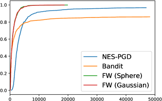
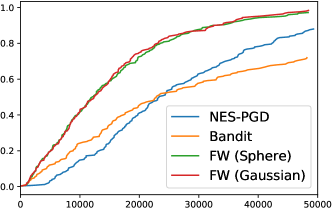
To provide more intuitive demonstrations, we also plot the attack success rate against the number of queries for our black-box experiments. Figure 1 shows the plots of the attack success rate against the number of queries for different algorithms on MNIST and ImageNet datasets respectively. As we can see from the plots, Bandit attack achieves better query efficiency for easy-to-attack examples (require less queries to attack) compared with NES-PGD or even FW at the early stages, but falls behind even to NES-PGD on hard-to-attack examples (require more queries to attack). We conjecture that in targeted attack setting, the gradient/data priors are not as accurate as in untargeted attack case, which makes Bandit attack less effective especially on hard-to-attack examples. On the other hand, our proposed Frank-Wolfe black-box attack algorithms achieve the highest attack success rate and the best efficiency (least queries needed for achieving the same success rate). This again confirm the advantage of Frank-Wolfe based projection-free algorithms for black-box attack.

(a) MNIST

(b) ImageNet

Figure 1: Attack success rate against the number of queries plot for targeted black-box attacks on MNIST and ImageNet datasets.

6 Conclusions and Future Work

In this work, we propose a Frank-Wolfe framework for efficient and effective adversarial attacks. Our proposed white-box and black-box attack algorithms enjoy an $O(1/\sqrt{T})$ rate of convergence, and the query complexity of the proposed black-box attack algorithm is linear in data dimension $d$. Finally, our empirical study on attacking both ImageNet dataset and MNIST dataset yield the best distortion in white-box setting and highest attack success rate/query complexity in black-box setting.

It would also be interesting to see the whether the performance of our Frank-Wolfe adversarial framework can be further improved by incorporating the idea of gradient/data priors (Ilyas et al., 2018b). We leave it as a future work.

Appendix A Derivation of LMO for General $p\geq 1$

The derivation of LMO is as follows: denote $\mathbf{h}=(\mathbf{x}-\mathbf{x}_{\rm{ori}})/\epsilon$, we have

$$\mathop{\mathrm{argmin}}_{\|\mathbf{x}-\mathbf{x}_{\rm{ori}}\|_{p}\leq\epsilon}\langle\mathbf{x},\mathbf{m}_{t}\rangle =\mathop{\mathrm{argmin}}_{\|\mathbf{h}\|_{p}\leq 1}\epsilon\cdot\langle\mathbf{h},\mathbf{m}_{t}\rangle$$

$$=\mathop{\mathrm{argmax}}_{\|\mathbf{h}\|_{p}\leq 1}\epsilon\cdot\langle\mathbf{h},-\mathbf{m}_{t}\rangle.$$

By Hölder’s inequality, the maximum value is reached when

$$|h_{i}|=c\cdot|(m_{t})_{i}|^{\frac{1}{p-1}},$$

where the subscript $i$ denotes the $i$-th element in the vector and $c$ is a universal constant. Together with the constraint of $\|\mathbf{h}\|_{p}\leq 1$ we obtain

$$h_{i}=-\frac{\mathop{\mathrm{sign}}\big{(}(m_{t})_{i}\big{)}\cdot|(m_{t})_{i}|^{\frac{1}{p-1}}}{\Big{(}\sum_{i=1}^{d}|(m_{t})_{i}|^{\frac{p}{p-1}}\Big{)}^{\frac{1}{p}}}$$

Therefore, we have

$$x_{i}=-\epsilon\cdot\frac{\mathop{\mathrm{sign}}\big{(}(m_{t})_{i}\big{)}\cdot|(m_{t})_{i}|^{\frac{1}{p-1}}}{\Big{(}\sum_{i=1}^{d}|(m_{t})_{i}|^{\frac{p}{p-1}}\Big{)}^{\frac{1}{p}}}+(x_{\rm{ori}})_{i}$$

Submit the above result back into LMO solution, for $p=2$ case, we have

$$\mathbf{v}_{t}=-\frac{\epsilon\cdot\mathbf{m}_{t}}{\|\mathbf{m}_{t}\|_{2}}+\mathbf{x}_{\rm{ori}}.$$

For $p=\infty$ case, we have

$$\mathbf{v}_{t}=-\epsilon\cdot\mathop{\mathrm{sign}}(\mathbf{m}_{t})+\mathbf{x}_{\rm{ori}}.$$

Appendix B Proof of the Main Results

In the section, we provide the proofs of the technical lemmas and theorems in the main paper.

B.1 Proof of Lemma 4.3

Proof.

By definition, we have

$$\|\nabla f(\mathbf{x}_{t})-\mathbf{m}_{t}\|_{2} =\|\nabla f(\mathbf{x}_{t})-\beta\mathbf{m}_{t-1}-(1-\beta)\nabla f(\mathbf{x}_{t})\|_{2}$$

$$=\beta\cdot\|\nabla f(\mathbf{x}_{t})-\mathbf{m}_{t-1}\|_{2}$$

$$=\beta\cdot\|\nabla f(\mathbf{x}_{t})-\nabla f(\mathbf{x}_{t-1})+\nabla f(\mathbf{x}_{t-1})-\mathbf{m}_{t-1}\|_{2}$$

$$\leq\beta\cdot\|\nabla f(\mathbf{x}_{t})-\nabla f(\mathbf{x}_{t-1})\|_{2}+\beta\cdot\|\nabla f(\mathbf{x}_{t-1})-\mathbf{m}_{t-1}\|_{2}$$

$$\leq\beta L\cdot\|\mathbf{x}_{t}-\mathbf{x}_{t-1}\|_{2}+\beta\cdot\|\nabla f(\mathbf{x}_{t-1})-\mathbf{m}_{t-1}\|_{2},$$ (B.1)

where the first inequality follows triangle inequality and the second inequality holds due to Assumption 4.1. In addition, we have the following result:

$$\|\mathbf{x}_{t}-\mathbf{x}_{t-1}\|_{2} =\gamma\|\mathbf{d}_{t-1}\|_{2}$$

$$=\gamma\|\mathbf{v}_{t-1}-\mathbf{x}_{t-1}\|_{2}$$

$$\leq\gamma D.$$ (B.2)

Substituting (B.2) into (B.1), and recursively applying the above inequality yields that

$$\|\nabla f(\mathbf{x}_{t})-\mathbf{m}_{t}\|_{2} \leq\gamma\big{(}\beta LD+\beta^{2}LD+\ldots+\beta^{t}\|\nabla f(\mathbf{x}_{0})-\mathbf{m}_{0}\|_{2}\big{)}$$

$$=\gamma\big{(}\beta LD+\beta^{2}LD+\ldots+\beta^{t-1}LD\big{)}$$

$$\leq\frac{\gamma LD}{1-\beta}.$$

∎

B.2 Proof of Theorem 4.4

Proof.

First by Assumption 4.1, we have

$$f(\mathbf{x}_{t+1}) \leq f(\mathbf{x}_{t})+\nabla f(\mathbf{x}_{t})^{\top}(\mathbf{x}_{t+1}-\mathbf{x}_{t})+\frac{L}{2}\|\mathbf{x}_{t+1}-\mathbf{x}_{t}\|_{2}^{2}$$

$$=f(\mathbf{x}_{t})+\gamma\nabla f(\mathbf{x}_{t})^{\top}(\mathbf{v}_{t}-\mathbf{x}_{t})+\frac{L\gamma^{2}}{2}\|\mathbf{v}_{t}-\mathbf{x}_{t}\|_{2}^{2}$$

$$\leq f(\mathbf{x}_{t})+\gamma\nabla f(\mathbf{x}_{t})^{\top}(\mathbf{v}_{t}-\mathbf{x}_{t})+\frac{LD^{2}\gamma^{2}}{2}$$

$$=f(\mathbf{x}_{t})+\gamma\mathbf{m}_{t}^{\top}(\mathbf{v}_{t}-\mathbf{x}_{t})+\gamma(\nabla f(\mathbf{x}_{t})-\mathbf{m}_{t})^{\top}(\mathbf{v}_{t}-\mathbf{x}_{t})+\frac{LD^{2}\gamma^{2}}{2},$$ (B.3)

where the last inequality uses the bounded domain condition in Assumption 4.2. Now define an auxiliary quantity:

$$\widehat{\mathbf{v}}_{t}=\mathop{\mathrm{argmin}}_{\mathbf{v}\in\mathcal{X}}\langle\mathbf{v},\nabla f(\mathbf{x}_{t})\rangle.$$

According to the definition of $g(\mathbf{x}_{t})$, this immediately implies

$$g(\mathbf{x}_{t})=-\langle\widehat{\mathbf{v}}_{t}-\mathbf{x}_{t},\nabla f(\mathbf{x}_{t})\rangle.$$ (B.4)

On the other hand, according to Line 5 in Algorithm 1, we have

$$\mathbf{v}_{t}=\mathop{\mathrm{argmin}}_{\mathbf{v}\in\mathcal{X}}\langle\mathbf{v},\mathbf{m}_{t}\rangle,$$

which implies that

$$\langle\mathbf{v}_{t},\mathbf{m}_{t}\rangle\leq\langle\widehat{\mathbf{v}}_{t},\mathbf{m}_{t}\rangle.$$ (B.5)

Combining (B.2) and (B.5), we further have

$$f(\mathbf{x}_{t+1}) \leq f(\mathbf{x}_{t})+\gamma\mathbf{m}_{t}^{\top}(\widehat{\mathbf{v}}_{t}-\mathbf{x}_{t})+\gamma(\nabla f(\mathbf{x}_{t})-\mathbf{m}_{t})^{\top}(\mathbf{v}_{t}-\mathbf{x}_{t})+\frac{LD^{2}\gamma^{2}}{2}$$

$$=f(\mathbf{x}_{t})+\gamma\nabla f(\mathbf{x}_{t})^{\top}(\widehat{\mathbf{v}}_{t}-\mathbf{x}_{t})+\gamma(\nabla f(\mathbf{x}_{t})-\mathbf{m}_{t})^{\top}(\mathbf{v}_{t}-\widehat{\mathbf{v}}_{t})+\frac{LD^{2}\gamma^{2}}{2}$$

$$=f(\mathbf{x}_{t})-\gamma g(\mathbf{x}_{t})+\gamma(\nabla f(\mathbf{x}_{t})-\mathbf{m}_{t})^{\top}(\mathbf{v}_{t}-\widehat{\mathbf{v}}_{t})+\frac{LD^{2}\gamma^{2}}{2}$$

$$\leq f(\mathbf{x}_{t})-\gamma g(\mathbf{x}_{t})+\gamma D\cdot\|\nabla f(\mathbf{x}_{t})-\mathbf{m}_{t}\|_{2}+\frac{LD^{2}\gamma^{2}}{2},$$ (B.6)

where the first equality is obtained by rearranging the second and the third term on the right hand side of the first inequality, the second equality follows the definition of the Frank-Wolfe gap $g(\mathbf{x}_{t})$ (B.4), and the last inequality holds due to Cauchy-Schwarz inequality. By Lemma 4.3, we have

$$\|\nabla f(\mathbf{x}_{t})-\mathbf{m}_{t}\|_{2} \leq\frac{\gamma LD}{1-\beta}.$$ (B.7)

Substituting (B.7) into (B.2), we obtain

$$f(\mathbf{x}_{t+1}) \leq f(\mathbf{x}_{t})-\gamma g(\mathbf{x}_{t})+\frac{LD^{2}\gamma^{2}}{1-\beta}+\frac{LD^{2}\gamma^{2}}{2}.$$

Telescoping over $t=0,\ldots,T-1$ of the above inequality, we obtain

$$f(\mathbf{x}_{T}) \leq f(\mathbf{x}_{0})-\sum_{t=0}^{T-1}\gamma g(\mathbf{x}_{t})+\frac{TLD^{2}\gamma^{2}}{1-\beta}+\frac{TLD^{2}\gamma^{2}}{2}.$$ (B.8)

Rearranging (B.8) yields

$$\frac{1}{T}\sum_{t=0}^{T-1}g(\mathbf{x}_{t}) \leq\frac{f(\mathbf{x}_{0})-f(\mathbf{x}_{T})}{T\gamma}+\gamma\bigg{(}\frac{LD^{2}}{1-\beta}+\frac{LD^{2}}{2}\bigg{)}$$

$$\leq\frac{f(\mathbf{x}_{0})-f(\mathbf{x}^{*})}{T\gamma}+\gamma\bigg{(}\frac{LD^{2}}{1-\beta}+\frac{LD^{2}}{2}\bigg{)},$$ (B.9)

where the second inequality is due to the optimality that $f(\mathbf{x}_{T})\geq f(\mathbf{x}^{*})$. (B.2) further implies

$$\widetilde{g}_{T}=\min_{1\leq k\leq T}g(\mathbf{x}_{k}) \leq\frac{f(\mathbf{x}_{0})-f(\mathbf{x}^{*})}{T\gamma}+\gamma\bigg{(}\frac{LD^{2}}{1-\beta}+\frac{LD^{2}}{2}\bigg{)}.$$

Let $\gamma=\sqrt{2(f(\mathbf{x}_{0})-f(\mathbf{x}^{*}))/(C_{\beta}LD^{2}T)}$ where $C_{\beta}=(3-\beta)/(1-\beta)$, we have

$$\widetilde{g}_{T} \leq\sqrt{\frac{2LD^{2}C_{\beta}(f(\mathbf{x}_{0})-f(\mathbf{x}^{*}))}{T}}.$$

∎

B.3 Proof of Lemma 4.7

Proof.

First, we have

$$\mathbb{E}\|\nabla f(\mathbf{x})-\mathbf{q}\|_{2} \leq\|\nabla f(\mathbf{x})-\mathbb{E}[\mathbf{q}]\|_{2}+\mathbb{E}\|\mathbf{q}-\mathbb{E}[\mathbf{q}]\|_{2}$$

$$\leq\underbrace{\|\nabla f(\mathbf{x})-\mathbb{E}[\mathbf{q}]\|_{2}}_{I_{1}}+\underbrace{\sqrt{\mathbb{E}\|\mathbf{q}-\mathbb{E}[\mathbf{q}]\|_{2}^{2}}}_{I_{2}},$$ (B.10)

where the first inequality follows from triangle inequality, the second inequality holds due to Jensen’s inequality. Let us denote $\bm{\psi}_{i}=\frac{d}{2\delta b}\big{(}f(\mathbf{x}+\delta\mathbf{u}_{i})-f(\mathbf{x}-\delta\mathbf{u}_{i})\big{)}\mathbf{u}_{i}$. For term $I_{1}$, we have

$$\mathbb{E}[\bm{\psi}_{i}] =\mathbb{E}_{\mathbf{u}}\bigg{[}\frac{d}{2\delta b}\big{(}f(\mathbf{x}+\delta\mathbf{u}_{i})-f(\mathbf{x}-\delta\mathbf{u}_{i})\big{)}\mathbf{u}_{i}\bigg{]}$$

$$=\mathbb{E}_{\mathbf{u}}\bigg{[}\frac{d}{2\delta b}f(\mathbf{x}+\delta\mathbf{u}_{i})\mathbf{u}_{i}\bigg{]}+\mathbb{E}_{\mathbf{u}}\bigg{[}\frac{d}{2\delta b}f(\mathbf{x}-\delta\mathbf{u}_{i})(-\mathbf{u}_{i})\bigg{]}$$

$$=\mathbb{E}_{\mathbf{u}}\bigg{[}\frac{d}{\delta b}f(\mathbf{x}+\delta\mathbf{u}_{i})\mathbf{u}_{i}\bigg{]}$$

$$=\frac{1}{b}\nabla f_{\delta}(\mathbf{x}),$$

where the third equality holds due to symmetric property of $\mathbf{u}_{i}$ and the last equality follows from Lemma C.1. Therefore, we have

$$\mathbb{E}[\mathbf{q}] =\mathbb{E}\bigg{[}\sum_{i=1}^{b}\bm{\psi}_{i}\bigg{]}=\nabla f_{\delta}(\mathbf{x}).$$

This further implies that

$$\|\nabla f(\mathbf{x})-\mathbb{E}[\mathbf{q}]\|_{2}=\|\nabla f(\mathbf{x})-\nabla f_{\delta}(\mathbf{x})\|_{2}\leq\frac{\delta dL}{2},$$ (B.11)

where the inequality follows from Lemma C.1.

For term $I_{2}$, note that $\bm{\psi}_{i}$’s are independent from each other due to the independence of $\mathbf{u}_{i}$, we have

$$\mathbb{E}\|\mathbf{q}-\mathbb{E}[\mathbf{q}]\|_{2}^{2} =\mathbb{E}\bigg{\|}\sum_{i=1}^{b}\Big{[}\bm{\psi}_{i}-\mathbb{E}\bm{\psi}_{i}\Big{]}\bigg{\|}_{2}^{2}$$

$$=\sum_{i=1}^{b}\mathbb{E}\big{\|}\bm{\psi}_{i}-\mathbb{E}\bm{\psi}_{i}\big{\|}^{2}\leq\sum_{i=1}^{b}\mathbb{E}\big{\|}\bm{\psi}_{i}\big{\|}^{2}.$$ (B.12)

Note that for term $\mathbb{E}\big{\|}\bm{\psi}_{i}\big{\|}^{2}$, we have

$$\mathbb{E}\big{\|}\bm{\psi}_{i}\big{\|}^{2} =\mathbb{E}_{\mathbf{u}}\bigg{\|}\frac{d}{2\delta b}\big{(}f(\mathbf{x}+\delta\mathbf{u}_{i})-f(\mathbf{x})+f(\mathbf{x})-f(\mathbf{x}-\delta\mathbf{u}_{i})\big{)}\mathbf{u}_{i}\bigg{\|}_{2}^{2}$$

$$\leq\frac{1}{2b^{2}}\mathbb{E}_{\mathbf{u}}\bigg{\|}\frac{d}{\delta}\big{(}f(\mathbf{x}+\delta\mathbf{u}_{i})-f(\mathbf{x})\big{)}\mathbf{u}_{i}\bigg{\|}_{2}^{2}+\frac{1}{2b^{2}}\mathbb{E}_{\mathbf{u}}\bigg{\|}\frac{d}{\delta}\big{(}f(\mathbf{x})-f(\mathbf{x}-\delta\mathbf{u}_{i})\big{)}\mathbf{u}_{i}\bigg{\|}_{2}^{2}$$

$$=\frac{1}{b^{2}}\mathbb{E}_{\mathbf{u}}\bigg{\|}\frac{d}{\delta}\big{(}f(\mathbf{x}+\delta\mathbf{u}_{i})-f(\mathbf{x})\big{)}\mathbf{u}_{i}\bigg{\|}_{2}^{2}$$

$$\leq\frac{1}{b^{2}}\bigg{(}2d\|\nabla f(\mathbf{x})\|_{2}^{2}+\frac{1}{2}\delta^{2}L^{2}d^{2}\bigg{)},$$ (B.13)

where the first inequality is due to the fact that $(a+b)^{2}\leq 2a^{2}+2b^{2}$, the second equality follows from the symmetric property of $\mathbf{u}_{i}$ and the last inequality is by Lemma C.1. Also note that by Assumption 4.1 and 4.6 we have

$$\|\nabla f(\mathbf{x})\|_{2}^{2}\leq(\|\nabla f({\bm{0}}))\|_{2}+L\|\mathbf{x}\|_{2})^{2}\leq(G+LD)^{2}.$$

Therefore, (B.3) can be further written as

$$\mathbb{E}\big{\|}\bm{\psi}_{i}\big{\|}^{2} \leq\frac{1}{b^{2}}\bigg{(}2d(G+LD)^{2}+\frac{1}{2}\delta^{2}L^{2}d^{2}\bigg{)}.$$ (B.14)

Substituting (B.14) into (B.3) we have

$$\mathbb{E}\|\mathbf{q}-\mathbb{E}[\mathbf{q}]\|_{2}^{2}\leq\frac{1}{b}\bigg{(}2d(G+LD)^{2}+\frac{1}{2}\delta^{2}L^{2}d^{2}\bigg{)}.$$ (B.15)

Combining (B.3), (B.11) and (B.15) we obtain

$$\mathbb{E}\|\nabla f(\mathbf{x})-\mathbf{q}\|_{2} \leq\frac{\delta Ld}{2}+\frac{1}{b}\bigg{(}2d(G+LD)^{2}+\frac{1}{2}\delta^{2}L^{2}d^{2}\bigg{)}$$

$$\leq\frac{\delta Ld}{2}+\frac{2\sqrt{d}(G+LD)+\delta Ld}{\sqrt{2b}}.$$

∎

B.4 Proof of Theorem 4.8

Proof.

First by Assumption 4.1, we have

$$f(\mathbf{x}_{t+1}) \leq f(\mathbf{x}_{t})+\nabla f(\mathbf{x}_{t})^{\top}(\mathbf{x}_{t+1}-\mathbf{x}_{t})+\frac{L}{2}\|\mathbf{x}_{t+1}-\mathbf{x}_{t}\|_{2}^{2}$$

$$=f(\mathbf{x}_{t})+\gamma\nabla f(\mathbf{x}_{t})^{\top}(\mathbf{v}_{t}-\mathbf{x}_{t})+\frac{L\gamma^{2}}{2}\|\mathbf{v}_{t}-\mathbf{x}_{t}\|_{2}^{2}$$

$$\leq f(\mathbf{x}_{t})+\gamma\nabla f(\mathbf{x}_{t})^{\top}(\mathbf{v}_{t}-\mathbf{x}_{t})+\frac{LD^{2}\gamma^{2}}{2}$$

$$=f(\mathbf{x}_{t})+\gamma\mathbf{m}_{t}^{\top}(\mathbf{v}_{t}-\mathbf{x}_{t})+\gamma(\nabla f(\mathbf{x}_{t})-\mathbf{m}_{t})^{\top}(\mathbf{v}_{t}-\mathbf{x}_{t})+\frac{LD^{2}\gamma^{2}}{2},$$ (B.16)

where the second inequality uses the bounded domain condition in Assumption 4.2. Now define an auxiliary quantity:

$$\widehat{\mathbf{v}}_{t}=\mathop{\mathrm{argmin}}_{\mathbf{v}\in\mathcal{X}}\langle\mathbf{v},\nabla f(\mathbf{x}_{t})\rangle.$$

According to the definition of $g(\mathbf{x}_{t})$, this immediately implies

$$g(\mathbf{x}_{t})=-\langle\widehat{\mathbf{v}}_{t}-\mathbf{x}_{t},\nabla f(\mathbf{x}_{t})\rangle.$$ (B.17)

On the other hand, according to Line 5 in Algorithm 1, we have

$$\mathbf{v}_{t}=\mathop{\mathrm{argmin}}_{\mathbf{v}\in\mathcal{X}}\langle\mathbf{v},\mathbf{m}_{t}\rangle,$$

which implies that

$$\langle\mathbf{v}_{t},\mathbf{m}_{t}\rangle\leq\langle\widehat{\mathbf{v}}_{t},\mathbf{m}_{t}\rangle.$$ (B.18)

Combining (B.4) and (B.18), we further have

$$f(\mathbf{x}_{t+1}) \leq f(\mathbf{x}_{t})+\gamma\mathbf{m}_{t}^{\top}(\widehat{\mathbf{v}}_{t}-\mathbf{x}_{t})+\gamma(\nabla f(\mathbf{x}_{t})-\mathbf{m}_{t})^{\top}(\mathbf{v}_{t}-\mathbf{x}_{t})+\frac{LD^{2}\gamma^{2}}{2}$$

$$=f(\mathbf{x}_{t})+\gamma\nabla f(\mathbf{x}_{t})^{\top}(\widehat{\mathbf{v}}_{t}-\mathbf{x}_{t})+\gamma(\nabla f(\mathbf{x}_{t})-\mathbf{m}_{t})^{\top}(\mathbf{v}_{t}-\widehat{\mathbf{v}}_{t})+\frac{LD^{2}\gamma^{2}}{2}$$

$$=f(\mathbf{x}_{t})-\gamma g(\mathbf{x}_{t})+\gamma(\nabla f(\mathbf{x}_{t})-\mathbf{m}_{t})^{\top}(\mathbf{v}_{t}-\widehat{\mathbf{v}}_{t})+\frac{LD^{2}\gamma^{2}}{2}$$

$$\leq f(\mathbf{x}_{t})-\gamma g(\mathbf{x}_{t})+\gamma D\cdot\|\nabla f(\mathbf{x}_{t})-\mathbf{m}_{t}\|_{2}+\frac{LD^{2}\gamma^{2}}{2},$$ (B.19)

where the first equality is obtained by rearranging the second and the third term on the right hand side of the first inequality, the second equality follows the definition of the Frank-Wolfe gap $g(\mathbf{x}_{t})$ (B.17), and the last inequality holds due to Cauchy-Schwarz inequality.

Take expectations for both sides of (B.4), we have

$$\mathbb{E}[f(\mathbf{x}_{t+1})] \leq\mathbb{E}[f(\mathbf{x}_{t})]-\gamma\mathbb{E}[g(\mathbf{x}_{t})]+\gamma D\cdot\mathbb{E}\|\nabla f(\mathbf{x}_{t})-\mathbf{m}_{t}\|_{2}+\frac{LD^{2}\gamma^{2}}{2}$$

$$\leq\mathbb{E}[f(\mathbf{x}_{t})]-\gamma\mathbb{E}[g(\mathbf{x}_{t})]+\gamma D\cdot\big{(}\mathbb{E}\|\mathbf{q}_{t}-\mathbf{m}_{t}\|_{2}+\|\nabla f(\mathbf{x}_{t})-\mathbf{q}_{t}\|_{2}\big{)}+\frac{LD^{2}\gamma^{2}}{2}$$

$$\leq\mathbb{E}[f(\mathbf{x}_{t})]-\gamma\mathbb{E}[g(\mathbf{x}_{t})]+\gamma D\Bigg{(}\mathbb{E}\|\mathbf{q}_{t}-\mathbf{m}_{t}\|_{2}+\frac{\delta Ld}{2}+\frac{2\sqrt{d}(G+LD)+\delta Ld}{\sqrt{2b}}\Bigg{)}+\frac{LD^{2}\gamma^{2}}{2},$$ (B.20)

where the second inequality follows from triangle inequality and the third inequality holds by Lemma 4.7. Similar to the proof of Lemma 4.3, we have

$$\mathbb{E}\|\mathbf{q}_{t}-\mathbf{m}_{t}\|_{2} \leq\beta\cdot\mathbb{E}\|\mathbf{q}_{t}-\mathbf{q}_{t-1}\|_{2}+\beta\cdot\mathbb{E}\|\mathbf{q}_{t-1}-\mathbf{m}_{t-1}\|_{2}$$

$$\leq\beta\big{(}\mathbb{E}\|\nabla f(\mathbf{x}_{t})-\mathbf{q}_{t}\|_{2}+\mathbb{E}\|\nabla f(\mathbf{x}_{t-1})-\mathbf{q}_{t-1}\|_{2}+\mathbb{E}\|\nabla f(\mathbf{x}_{t})-\nabla f(\mathbf{x}_{t-1})\|_{2}\big{)}+\beta\cdot\mathbb{E}\|\mathbf{q}_{t-1}-\mathbf{m}_{t-1}\|_{2}$$

$$\leq\beta\bigg{(}\delta Ld+\frac{2\sqrt{2d}(G+LD)+\sqrt{2}\delta Ld}{\sqrt{b}}+L\|\mathbf{x}_{t}-\mathbf{x}_{t-1}\|_{2}\bigg{)}+\beta\cdot\mathbb{E}\|\mathbf{q}_{t-1}-\mathbf{m}_{t-1}\|_{2}$$

$$\leq\beta\bigg{(}\delta Ld+\frac{2\sqrt{2d}(G+LD)+\sqrt{2}\delta Ld}{\sqrt{b}}+\gamma LD\bigg{)}+\beta\cdot\mathbb{E}\|\mathbf{q}_{t-1}-\mathbf{m}_{t-1}\|_{2},$$ (B.21)

where the first and the second inequalities follow from triangle inequality, the third inequality follows from Lemma 4.7, and the last inequality follows from (B.2). Recursively applying (B.4) yields that

$$\mathbb{E}\|\mathbf{q}_{t}-\mathbf{m}_{t}\|_{2} \leq\frac{1}{1-\beta}\bigg{(}\delta Ld+\frac{2\sqrt{2d}(G+LD)+\sqrt{2}\delta Ld}{\sqrt{b}}+\gamma LD\bigg{)}.$$ (B.22)

Combining (B.4) and (B.22), we have

$$\mathbb{E}[f(\mathbf{x}_{t+1})] \leq\mathbb{E}[f(\mathbf{x}_{t})]-\gamma\mathbb{E}[g(\mathbf{x}_{t})]+\frac{LD^{2}\gamma^{2}}{2}+\gamma D\cdot\Bigg{(}\frac{3-\beta}{1-\beta}\bigg{(}\frac{\delta Ld}{2}+\frac{2\sqrt{d}(G+LD)+\delta Ld}{\sqrt{2b}}\bigg{)}+\frac{\gamma LD}{1-\beta}\Bigg{)}.$$ (B.23)

Telescoping over $t$ of (B.23), we obtain

$$\mathbb{E}[f(\mathbf{x}_{T})] \leq f(\mathbf{x}_{0})-\sum_{t=0}^{T-1}\gamma\mathbb{E}[g(\mathbf{x}_{t})]+\frac{TLD^{2}\gamma^{2}}{2}+\gamma DT\Bigg{(}\frac{3-\beta}{1-\beta}\bigg{(}\frac{\delta Ld}{2}+\frac{2\sqrt{d}(G+LD)+\delta Ld}{\sqrt{2b}}\bigg{)}+\frac{\gamma LD}{1-\beta}\Bigg{)}.$$ (B.24)

Rearranging (B.24) yields

$$\frac{1}{T}\sum_{t=0}^{T-1}\mathbb{E}[g(\mathbf{x}_{t})] \leq\frac{f(\mathbf{x}_{0})-\mathbb{E}[f(\mathbf{x}_{T})]}{T\gamma}+D\cdot\frac{3-\beta}{1-\beta}\bigg{(}\gamma LD+\frac{\delta Ld}{2}+\frac{2\sqrt{d}(G+LD)+\delta Ld}{\sqrt{2b}}\bigg{)}$$

$$\leq\frac{f(\mathbf{x}_{0})-f(\mathbf{x}^{*})}{T\gamma}+D\cdot\frac{3-\beta}{1-\beta}\bigg{(}\gamma LD+\frac{\delta Ld}{2}+\frac{2\sqrt{d}(G+LD)+\delta Ld}{\sqrt{2b}}\bigg{)},$$ (B.25)

where the second inequality is due to the optimality that $f(\mathbf{x}_{T})\geq f(\mathbf{x}^{*})$. By the definition of $\widetilde{g}_{T}$ in Algorithm 2, we further have

$$\mathbb{E}[\widetilde{g}_{T}] \leq\frac{f(\mathbf{x}_{0})-f(\mathbf{x}^{*})}{T\gamma}+D\cdot\frac{3-\beta}{1-\beta}\bigg{(}\gamma LD+\frac{\delta Ld}{2}+\frac{2\sqrt{d}(G+LD)+\delta Ld}{\sqrt{2b}}\bigg{)}.$$

Let $\gamma=\sqrt{(f(\mathbf{x}_{0})-f(\mathbf{x}^{*}))/(C_{\beta}LD^{2}T)}$ where $C_{\beta}=(3-\beta)/(1-\beta)$, $b=Td$ and $\delta=\sqrt{1/(Td^{2})}$, we have

$$\mathbb{E}[\widetilde{g}_{T}] \leq\frac{f(\mathbf{x}_{0})-f(\mathbf{x}^{*})}{T\gamma}+C_{\beta}LD^{2}\gamma+C_{\beta}D\Bigg{(}\frac{\delta Ld}{2}+\frac{2\sqrt{d}(G+LD)+\delta Ld}{\sqrt{2b}}\Bigg{)}$$

$$\leq\frac{D}{\sqrt{T}}\Big{(}2\sqrt{C_{\beta}L(f(\mathbf{x}_{0})-f(\mathbf{x}^{*}))}+C_{\beta}(L+G+LD)\Big{)}.$$

∎

Appendix C Auxiliary Lemma

Lemma C.1 (Lemma 4.1 in Gao et al. (2018)).

Under Assumption 4.1, let $f_{\delta}(\mathbf{x})=\mathbb{E}_{\mathbf{u}}[f(\mathbf{x}+\delta\mathbf{u})]$ where $\mathbf{u}$ is sampled uniformly from the Euclidean unit sphere with with $\|\mathbf{u}\|_{2}=1$, we have

$$\nabla f_{\delta}(\mathbf{x})=\mathbb{E}_{\mathbf{u}}\bigg{[}\frac{d}{\delta}f(\mathbf{x}+\delta\mathbf{u})\mathbf{u}\bigg{]},$$

$$\|\nabla f(\mathbf{x})-\nabla f_{\delta}(\mathbf{x})\|_{2}\leq\frac{\delta dL}{2},$$

$$\mathbb{E}_{\mathbf{u}}\bigg{\|}\frac{d}{\delta}\big{(}f(\mathbf{x}+\delta\mathbf{u})-f(\mathbf{x})\big{)}\mathbf{u}\bigg{\|}_{2}^{2}=\bigg{(}2d\|\nabla f(\mathbf{x})\|_{2}^{2}+\frac{1}{2}\delta^{2}L^{2}d^{2}\bigg{)},$$

where $L$ is the smoothness parameter and $d$ is the data dimension.

Appendix D Additional Experimental Details

D.1 Parameter Settings

As we mentioned in the main paper, we performed grid search to tune the hyper-parameters for all algorithm to ensure a fair comparison. In detail, in white-box experiments, for Algorithm 1, we tune the step size $\gamma_{t}$ by searching the grid $\{0.1,0.2,\ldots,0.9\}$ on both datasets. For PGD and MI-FGSM, we tune the learning rate by searching the grid $\{0.05,0.10,\ldots,0.25,0.30\}$ on MNIST and $\{0.01,0.02,\ldots,0.4,0.5]$ on ImageNet. For both FW and MI-FGSM, we tune the momentum parameter $\beta$ by searching the grid $\{0.1,0.5,0.9,0.99\}$. In black-box experiments, for Algorithm 2, we tune the step size $\gamma_{t}$ by the grid $\{0.1/\sqrt{t},0.2/\sqrt{t},\ldots,0.9/\sqrt{t}\}$, the momentum parameter $\beta$ by the grid $\{0.5,0.9,0.99,0.999,0.9999\}$, the sample size for gradient estimation $b$ by the grid $\{5,10,\ldots,50\}$, and the sampling parameter $\delta$ by the grid $\{0.1,0.01,0.001,0.0001\}$. For NES-PGD and Bandit, we tune the learning rate by the grid $\{0.01,0.02,\ldots,0.10\}$ on MNIST and $\{0.001,0.005,0.01,\ldots,0.02\}$ on ImageNet. For other parameters, we follow the recommended parameter setting in their original papers. We report the hyperparameters tuned by grid search in the sequel. In detail, for white-box experiments, we list the hyper-parameters used for all algorithms in Table 4. For black-box experiments, we list the hyper-parameters for Frank-Wolfe black-box attack algorithm in Table 5. We also list the hyper-parameters used for NES-PGD and Bandit black-box attack algorithms in Tables 6 and 7 respectively.

Table 4: Parameters used in targeted white-box experiments.

Parameters	MNIST			ImageNet
	PGD	MI-FGSM	FW	PGD	MI-FGSM	FW
$\epsilon$	0.3			0.05
$\gamma_{t}$	0.1	0.1	0.5	0.03	0.03	0.1
$\beta$	-	0.9	0.9	-	0.9	0.9

Table 5: Parameters used in Frank-Wolfe black-box experiments.

Parameter	MNIST	ImageNet
$\{\gamma_{t}\}$	$0.8/\sqrt{t}$	$0.8/\sqrt{t}$
$\beta$	0.99	0.999
$b$	25	25
$\delta$	0.01	0.01

Table 6: Parameters used in NES-PGD black-box experiments.

Parameter	MNIST	ImageNet
learning rate	$0.02$	$0.005$
number of finite difference estimations per step	25	25
finite difference probe	0.001	0.001

Table 7: Parameters used in Bandit black-box experiments.

Parameter	MNIST	ImageNet
learning rate	$0.03$	$0.01$
finite difference probe	0.1	0.1
online convex optimization learning rate	0.001	0.0001
data-dependent prior size	8	50
bandit exploration	0.01	0.01

References

- Bahdanau et al. (2016) Bahdanau, D., Chorowski, J., Serdyuk, D., Brakel, P. and Bengio, Y. (2016). End-to-end attention-based large vocabulary speech recognition. In Acoustics, Speech and Signal Processing (ICASSP), 2016 IEEE International Conference on. IEEE.
- Balasubramanian and Ghadimi (2018) Balasubramanian, K. and Ghadimi, S. (2018). Zeroth-order (non)-convex stochastic optimization via conditional gradient and gradient updates. arXiv preprint arXiv:1809.06474 .
- Bhagoji et al. (2017) Bhagoji, A. N., He, W., Li, B. and Song, D. (2017). Exploring the space of black-box attacks on deep neural networks. arXiv preprint arXiv:1712.09491 .
- Boyd and Vandenberghe (2004) Boyd, S. and Vandenberghe, L. (2004). Convex optimization. Cambridge university press.
- Carlini et al. (2016) Carlini, N., Mishra, P., Vaidya, T., Zhang, Y., Sherr, M., Shields, C., Wagner, D. and Zhou, W. (2016). Hidden voice commands. In USENIX Security Symposium.
- Carlini and Wagner (2017) Carlini, N. and Wagner, D. (2017). Towards evaluating the robustness of neural networks. In 2017 IEEE Symposium on Security and Privacy (SP). IEEE.
- Chen et al. (2017a) Chen, H., Zhang, H., Chen, P.-Y., Yi, J. and Hsieh, C.-J. (2017a). Show-and-fool: Crafting adversarial examples for neural image captioning. arXiv preprint arXiv:1712.02051 .
- Chen et al. (2017b) Chen, P.-Y., Sharma, Y., Zhang, H., Yi, J. and Hsieh, C.-J. (2017b). Ead: elastic-net attacks to deep neural networks via adversarial examples. arXiv preprint arXiv:1709.04114 .
- Chen et al. (2017c) Chen, P.-Y., Zhang, H., Sharma, Y., Yi, J. and Hsieh, C.-J. (2017c). Zoo: Zeroth order optimization based black-box attacks to deep neural networks without training substitute models. In Proceedings of the 10th ACM Workshop on Artificial Intelligence and Security. ACM.
- Cheng et al. (2018) Cheng, M., Yi, J., Zhang, H., Chen, P.-Y. and Hsieh, C.-J. (2018). Seq2sick: Evaluating the robustness of sequence-to-sequence models with adversarial examples. arXiv preprint arXiv:1803.01128 .
- Deng et al. (2009) Deng, J., Dong, W., Socher, R., Li, L.-J., Li, K. and Fei-Fei, L. (2009). Imagenet: A large-scale hierarchical image database. In Computer Vision and Pattern Recognition, 2009. CVPR 2009. IEEE Conference on. Ieee.
- Dong et al. (2018) Dong, Y., Liao, F., Pang, T., Su, H., Zhu, J., Hu, X. and Li, J. (2018). Boosting adversarial attacks with momentum. In Proceedings of the IEEE conference on computer vision and pattern recognition.
- Flaxman et al. (2005) Flaxman, A. D., Kalai, A. T. and McMahan, H. B. (2005). Online convex optimization in the bandit setting: gradient descent without a gradient. In Proceedings of the sixteenth annual ACM-SIAM symposium on Discrete algorithms. Society for Industrial and Applied Mathematics.
- Frank and Wolfe (1956) Frank, M. and Wolfe, P. (1956). An algorithm for quadratic programming. Naval research logistics quarterly 3 95–110.
- Gao et al. (2018) Gao, X., Jiang, B. and Zhang, S. (2018). On the information-adaptive variants of the admm: an iteration complexity perspective. Journal of Scientific Computing 76 327–363.
- Girshick (2015) Girshick, R. (2015). Fast r-cnn. In Proceedings of the IEEE international conference on computer vision.
- Goodfellow et al. (2015) Goodfellow, I. J., Shlens, J. and Szegedy, C. (2015). Explaining and harnessing adversarial examples. ICLR .
- He et al. (2016) He, K., Zhang, X., Ren, S. and Sun, J. (2016). Deep residual learning for image recognition. In CVPR.
- Hu and Tan (2017) Hu, W. and Tan, Y. (2017). Generating adversarial malware examples for black-box attacks based on gan. arXiv preprint arXiv:1702.05983 .
- Ilyas et al. (2018a) Ilyas, A., Engstrom, L., Athalye, A., Lin, J., Athalye, A., Engstrom, L., Ilyas, A. and Kwok, K. (2018a). Black-box adversarial attacks with limited queries and information. In Proceedings of the 35th International Conference on Machine Learning,ICML 2018.
- Ilyas et al. (2018b) Ilyas, A., Engstrom, L. and Madry, A. (2018b). Prior convictions: Black-box adversarial attacks with bandits and priors. arXiv preprint arXiv:1807.07978 .
- Jaggi (2013) Jaggi, M. (2013). Revisiting frank-wolfe: Projection-free sparse convex optimization. In ICML (1).
- Kingma and Ba (2015) Kingma, D. P. and Ba, J. (2015). Adam: A method for stochastic optimization. International Conference on Learning Representations .
- Krizhevsky et al. (2012) Krizhevsky, A., Sutskever, I. and Hinton, G. E. (2012). Imagenet classification with deep convolutional neural networks. In Advances in neural information processing systems.
- Kurakin et al. (2016) Kurakin, A., Goodfellow, I. and Bengio, S. (2016). Adversarial examples in the physical world. arXiv preprint arXiv:1607.02533 .
- Lacoste-Julien (2016) Lacoste-Julien, S. (2016). Convergence rate of frank-wolfe for non-convex objectives. arXiv preprint arXiv:1607.00345 .
- LeCun (1998) LeCun, Y. (1998). The mnist database of handwritten digits. http://yann.lecun.com/exdb/mnist/ .
- Liu et al. (2018) Liu, Y., Chen, X., Liu, C. and Song, D. (2018). Delving into transferable adversarial examples and black-box attacks. International Conference on Data Mining (ICDM) .
- Madry et al. (2018) Madry, A., Makelov, A., Schmidt, L., Tsipras, D. and Vladu, A. (2018). Towards deep learning models resistant to adversarial attacks. International Conference on Learning Representations .
- Mohamed et al. (2012) Mohamed, A.-r., Dahl, G. E., Hinton, G. et al. (2012). Acoustic modeling using deep belief networks. IEEE Trans. Audio, Speech & Language Processing 20 14–22.
- Moosavi-Dezfooli et al. (2016) Moosavi-Dezfooli, S.-M., Fawzi, A. and Frossard, P. (2016). Deepfool: a simple and accurate method to fool deep neural networks. In Proceedings of the IEEE Conference on Computer Vision and Pattern Recognition.
- Papernot et al. (2016a) Papernot, N., McDaniel, P. and Goodfellow, I. (2016a). Transferability in machine learning: from phenomena to black-box attacks using adversarial samples. arXiv preprint arXiv:1605.07277 .
- Papernot et al. (2017) Papernot, N., McDaniel, P., Goodfellow, I., Jha, S., Celik, Z. B. and Swami, A. (2017). Practical black-box attacks against machine learning. In Proceedings of the 2017 ACM on Asia Conference on Computer and Communications Security. ACM.
- Papernot et al. (2016b) Papernot, N., McDaniel, P., Jha, S., Fredrikson, M., Celik, Z. B. and Swami, A. (2016b). The limitations of deep learning in adversarial settings. In Security and Privacy (EuroS&P), 2016 IEEE European Symposium on. IEEE.
- Pattanaik et al. (2018) Pattanaik, A., Tang, Z., Liu, S., Bommannan, G. and Chowdhary, G. (2018). Robust deep reinforcement learning with adversarial attacks. In Proceedings of the 17th International Conference on Autonomous Agents and MultiAgent Systems. International Foundation for Autonomous Agents and Multiagent Systems.
- Reddi et al. (2016) Reddi, S. J., Sra, S., Póczos, B. and Smola, A. (2016). Stochastic frank-wolfe methods for nonconvex optimization. In Communication, Control, and Computing (Allerton), 2016 54th Annual Allerton Conference on. IEEE.
- Ren et al. (2015) Ren, S., He, K., Girshick, R. and Sun, J. (2015). Faster r-cnn: Towards real-time object detection with region proposal networks. In Advances in neural information processing systems.
- Salimans et al. (2017) Salimans, T., Ho, J., Chen, X., Sidor, S. and Sutskever, I. (2017). Evolution strategies as a scalable alternative to reinforcement learning. arXiv preprint arXiv:1703.03864 .
- Santurkar et al. (2018) Santurkar, S., Tsipras, D., Ilyas, A. and Madry, A. (2018). How does batch normalization help optimization?(no, it is not about internal covariate shift). arXiv preprint arXiv:1805.11604 .
- Shamir (2017) Shamir, O. (2017). An optimal algorithm for bandit and zero-order convex optimization with two-point feedback. Journal of Machine Learning Research 18 1–11.
- Sinha et al. (2018) Sinha, A., Namkoong, H. and Duchi, J. (2018). Certifying some distributional robustness with principled adversarial training. International Conference on Learning Representations .
- Staib and Jegelka (2017) Staib, M. and Jegelka, S. (2017). Distributionally robust deep learning as a generalization of adversarial training. Machine Learning and Computer Security Workshop .
- Szegedy et al. (2016) Szegedy, C., Vanhoucke, V., Ioffe, S., Shlens, J. and Wojna, Z. (2016). Rethinking the inception architecture for computer vision. In Proceedings of the IEEE conference on computer vision and pattern recognition.
- Szegedy et al. (2013) Szegedy, C., Zaremba, W., Sutskever, I., Bruna, J., Erhan, D., Goodfellow, I. and Fergus, R. (2013). Intriguing properties of neural networks. arXiv preprint arXiv:1312.6199 .
- Tu et al. (2018) Tu, C., Ting, P., Chen, P., Liu, S., Zhang, H., Yi, J., Hsieh, C. and Cheng, S. (2018). Autozoom: Autoencoder-based zeroth order optimization method for attacking black-box neural networks. CoRR abs/1805.11770.
- Wierstra et al. (2014) Wierstra, D., Schaul, T., Glasmachers, T., Sun, Y., Peters, J. and Schmidhuber, J. (2014). Natural evolution strategies. The Journal of Machine Learning Research 15 949–980.
- Xu et al. (2017) Xu, X., Chen, X., Liu, C., Rohrbach, A., Darell, T. and Song, D. (2017). Can you fool ai with adversarial examples on a visual turing test? arXiv preprint arXiv:1709.08693 .
- Yu et al. (2017) Yu, Y., Zhang, X. and Schuurmans, D. (2017). Generalized conditional gradient for sparse estimation. The Journal of Machine Learning Research 18 5279–5324.