Entanglement properties of a measurement-based entanglement distillation experiment

Abstract

Measures of entanglement can be employed for the analysis of numerous quantum information protocols. Due to computational convenience, logarithmic negativity is often the choice in the case of continuous variable systems. In this work, we analyse a continuous variable measurement-based entanglement distillation experiment using a collection of entanglement measures. This includes: logarithmic negativity, entanglement of formation, distillable entanglement, relative entropy of entanglement, and squashed entanglement. By considering the distilled entanglement as a function of the success probability of the distillation protocol, we show that the logarithmic negativity surpasses the bound on deterministic entanglement distribution at a relatively large probability of success. This is in contrast to the other measures which would only be able to do so at much lower probabilities, hence demonstrating that logarithmic negativity alone is inadequate for assessing the performance of the distillation protocol. In addition to this result, we also observed an increase in the distillable entanglement by making use of upper and lower bounds to estimate this quantity. We thus demonstrate the utility of these theoretical tools in an experimental setting.

I Introduction

On the one hand, quantum entanglement is a useful non-classical resource. It can be used for the construction of quantum gates Menicucci et al. (2006), or for the distribution of cryptographic keys in a secure manner Scarani et al. (2009). On the other hand, implementations of these tasks are usually limited in performance due to experimental imperfections. Utilising a variety of methods such as photon subtraction Takahashi et al. (2010); Kurochkin et al. (2014) and noiseless linear amplification Chrzanowski et al. (2014); Ulanov et al. (2015), entanglement distillation protocols seek a potential resolution to this problem by concentrating weakly entangled states into subsets that are more entangled.

Here we address the problem of quantifying entanglement distillation; this will, in general, depend on the kind of system that one is working with. In the case of discrete variables, the fidelity with respect to some maximally entangled state Pan et al. (2003) and non-locality based on the Bell inequalities Kwiat et al. (2001) are both useful measures for observing quantum entanglement. However, these methods are not particularly suitable in the case of continuous variables. Maximally entangled continuous variable states do not exist, and a theorem due to Bell precludes the demonstration of non-locality using Gaussian states and Gaussian measurements (the standard tools for continuous variable experiments) Bell (2004), unless one introduces additional assumptions on one’s system Thearle et al. (2018); Ralph et al. (2000). Thus far, the analyses of continuous variable entanglement distillation have instead centred around inseparability criteria Simon (2000); Duan et al. (2000) and, most notably, the logarithmic negativity Vidal and Werner (2002) as one can calculate it quite straightforwardly.

In this work, we analyse a continuous variable measurement-based entanglement distillation experiment Chrzanowski et al. (2014) using a collection of measures. We present two main results. First, we show that the logarithmic negativity is distinct from the other measures; it crosses the “deterministic bound” before the other measures do, at a probability of success (of the distillation protocol) that is orders of magnitude greater. The deterministic bound is the maximum entanglement that can be deterministically distributed across a given quantum channel (usually imperfect), assuming that one had an EPR resource state with infinite squeezing. For instance, when the entanglement of formation crosses this bound, we can take it to indicate a form of error correction Tserkis et al. (2018), thus giving an example of how the logarithmic negativity can fail to capture important properties of distillation protocols. Our results can be regarded as an experimental demonstration of such an example.

Our second result is the certification of an increase in the distillable entanglement. Currently, there is no known way for evaluating the distillable entanglement directly, which means that one is only able to look at it through the use of upper and lower bounds Dong et al. (2010, 2008). The upper bound puts a limit on how much distillable entanglement we had prior to distillation, while the lower bound guarantees at least how much we have after performing distillation. By observing a sufficient increase in the lower bound, we could certify that the distillable entanglement has indeed increased. We remark that the minimisation of optical loss and the choice of a sharp upper bound turned out to be important factors in order to observe the increase in the distillable entanglement. In particular, there are many possible choices for the upper bound, but the relative entropy of entanglement was found to be the only one that was sufficiently stringent for this task.

We have organised this paper as follows. In section II, we provide some background in Gaussian quantum optics, and establish the notations and conventions that will be used throughout this paper. In section III, definitions of the various entanglement measures are provided, discussing their basic properties with an emphasis on operational interpretations. In section IV, the final section, we briefly describe the experiment setup and present a discussion of the distillation results based on the measures.

II Preliminaries

Gaussian states can be characterised by the first and second moments of the quadrature operators Weedbrook et al. (2012) — also known respectively as the mean fields and the covariance matrix. Since measures of entanglement depend only on the covariance matrix, we will assume vanishing mean fields without the loss of generality. For two-mode Gaussian states, the covariance matrix can be written in block form (using the $xpxp$ notation Ukai (2015)):

$$\sigma=\begin{bmatrix}M&C\\ C^{T}&N\end{bmatrix},$$

where $M$, $N$, and $C$ are real $2\times 2$ matrices. In general, the entries of the covariance matrix depend on the value of $\hbar$; in this paper, we will normalise to the variance of the vacuum field, which amounts to setting $\hbar=2$. In order for the covariance matrix to represent a physical state, it is also required to satisfy the Heisenberg uncertainty principle.

The density matrix of closed quantum systems evolve under unitaries: $\hat{\rho}\rightarrow\hat{U}\hat{\rho}\hat{U}^{\dagger}$. In general, representations of these unitaries in the Fock basis require infinite-dimensional matrices; if we restrict ourselves to Gaussian operations, this can be simplified to the evolution of covariance matrices: $\sigma\rightarrow S\sigma S^{T}$. For two-mode states, each $S$ is a $4\times 4$ square matrix and is symplectic with respect to the following symplectic form:

$$\Omega=\begin{bmatrix}0&1&0&0\\ -1&0&0&0\\ 0&0&0&1\\ 0&0&-1&0\\ \end{bmatrix}.$$

It satisfies the equation $S\Omega S^{T}=\Omega$. Every Gaussian unitary $\hat{U}$ is associated with a symplectic matrix. We will find the following unitary useful:

$$\hat{S}_{2}(r)=e^{r(\hat{a}\hat{b}-\hat{a}^{\dagger}\hat{b}^{\dagger})/2},$$ (1)

which is known as the two-mode-squeezing operator. As usual, $\hat{a}$ and $\hat{b}$ denote the annihilation operators of the two optical modes. The two-mode-squeezing operator is parametrised by the squeezing parameter $r$, with $r=0$ corresponding to no squeezing and $r\rightarrow\infty$ to the limit of infinite squeezing.

Any given covariance matrix $\sigma$ can be put into the following standard form:

$$\sigma=\begin{bmatrix}m&0&c_{1}&0\\ 0&m&0&c_{2}\\ c_{1}&0&n&0\\ 0&c_{2}&0&n\end{bmatrix},$$ (2)

and this can be done using only local Gaussian unitaries Duan et al. (2000), which does not change the entanglement of the state.

One can always diagonalise the covariance matrix using only symplectic matrices, and the corresponding eigenvalues are called symplectic eigenvalues Williamson (1936). Of particular importance are the symplectic eigenvalues of the partially transposed state. For two-mode Gaussian states, the partial transpose flips the sign of the phase quadrature, equivalent to flipping the sign of the $c_{2}$ entry in the standard form of the covariance matrix (Eq. 2). The symplectic eigenvalues $\tilde{\nu}_{\pm}$ of the partially transposed state are given by

$$\tilde{\nu}_{\pm}^{2}=\frac{\tilde{\Delta}\pm\sqrt{\tilde{\Delta}^{2}-4\det\sigma}}{2},$$ (3)

where $\tilde{\Delta}=\det M+\det N-2\det C$.

For convenience, covariance matrices of the form

$$\sigma=\begin{bmatrix}m&0&c&0\\ 0&m&0&-c\\ c&0&m&0\\ 0&-c&0&m\end{bmatrix}$$ (4)

will be called symmetric, while those of the form

$$\sigma=\begin{bmatrix}m&0&c&0\\ 0&m&0&-c\\ c&0&n&0\\ 0&-c&0&n\end{bmatrix}$$ (5)

will be called quadrature-symmetric. These states form strict subsets of general two-mode Gaussian states (Eq. 2) by imposing different kinds of symmetries.

III Entanglement measures

We present some background on the theory of entanglement measures, including definitions, properties, and formulae that will be useful. We note that the problem of computing entanglement measures is NP-complete for many measures Huang (2014), with analytical expressions available only in restricted cases that will generally possess some degree of symmetry. In the special case of the entanglement of formation, such a restriction will give rise to a simple operational interpretation in terms of quantum squeezing, and thus a connection to the logarithmic negativity which we briefly discuss.

III.1 Entanglement entropy

The entanglement entropy $\mathcal{E}_{V}$ uniquely determines entanglement on the set of pure states. Given the von Neumann entropy $S$, with

$$S(\hat{\rho})=-tr(\hat{\rho}\log\hat{\rho}),$$ (6)

the entanglement entropy $\mathcal{E}_{V}$ is defined to be the von Neumann entropy of the reduced states Bennett et al. (1996a):

$$\mathcal{E}_{V}(\left|\psi\right>)=S(\hat{\rho}_{A})=S(\hat{\rho}_{B}).$$ (7)

The subscripts $A$ and $B$ denote the two subsystems of $\left|\psi\right>$: $\hat{\rho}_{A}=tr_{B}(\left|\psi\right>\left<\psi\right|)$ and $\hat{\rho}_{B}=tr_{A}(\left|\psi\right>\left<\psi\right|)$. For Gaussian states, the von Neumann entropy depends only on the symplectic eigenvalues of the covariance matrix. Throughout this paper, logarithms are taken with respect to base $e$.

III.2 Entanglement cost and distillable entanglement

Figure 1: An ordering of the measures. If a measure $A$ sits above $B$ with a line connecting them, then $A(\hat{\rho})\geq B(\hat{\rho})$ for all states $\hat{\rho}$. If one considers only pure states, then all measures shown in the diagram (except the logarithmic negativity) reduces to the entanglement entropy. When restricting to pure two-mode Gaussian states, the logarithmic negativity and the entanglement entropy can also be regarded as equivalent in the sense of Eq. 13. Citations in the figure refer to proofs for each inequality.

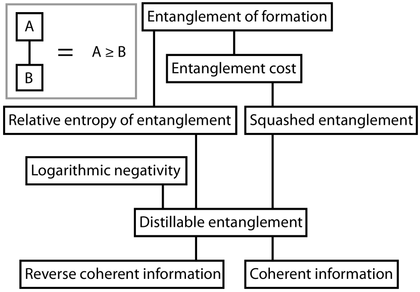
The extension of the entanglement entropy to mixed states is not unique. Two possible choices are the entanglement cost and the distillable entanglement; they are quite fundamental, since they represent, respectively, the average pure state entanglement that is needed for or that can be extracted from any given state (usually mixed). The precise definitions are quite cumbersome to state and somewhat unecessary for this paper, but they can be found in, for instance, Horodecki et al. Horodecki et al. (2009). The entanglement cost is an upper bound to the distillable entanglement (Fig. 1), and they both reduce to the entanglement entropy on the set of pure states. Neither measure is straightforward to compute in general.

The entanglement cost is the asymptotic (regularized) version of the entanglement of formation Hayden et al. (2001), which can be computed for two-mode Gaussian states and is discussed in the next subsection. It follows from this regularisation formula (and the sub-additivity of the von Neumann entropy) that the entanglement of formation bounds the entanglement cost from above Hayden et al. (2001); Araki and Lieb (1970); in fact, recent work shows that the two quantities coincide on a subset of states Wilde , but the extent to which their equivalence holds is presently unknown.

The distillable entanglement, on the other hand, does not admit any closed expressions that we can evaluate straightforwardly. It can be upper bounded by a number of quantities (see Fig. 1): the entanglement of formation Bennett et al. (1996b), the relative entropy of entanglement Vedral and Plenio (1998), the squashed entanglement Christandl and Winter (2004), and the logarithmic negativity Vidal and Werner (2002); it also admits lower bounds due to the coherent and reverse coherent information Devetak and Winter (2005). We shall find such bounds useful for estimating the distillable entanglement.

III.3 Entanglement of formation

[figure]style=plain,subcapbesideposition=top

Figure 2: A comparison of the logarithmic negativity (equivalently, the PPT criterion) and the entanglement of formation. The operational interpretations of the two measures can be illustrated in terms of quantum squeezing, and the picture above holds good for two-mode Gaussian states that are symmetric in quadratures (those represented by Eq. 5). The minimum two-mode squeezing required to produce the entangled state corresponds to the entanglement of formation, while the maximum local squeezing that can be extracted from the entangled state can be identified with the symplectic eigenvalue $\tilde{\nu}_{-}$, and hence with the logarithmic negativity as well. The decomposition of two-mode squeezing into single-mode squeezers and passive operations has been shown explicitly; in addition, the beam-splitting ratio $T$ that achieves maximal local squeezing will, in general, be state-dependent. The separable resource need not be symmetric (i.e. of the form in Eq. 4) if the entangled state is not, and can also support non-vanishing correlations across the two modes as long as it remains separable.

The entanglement of formation measures the minimum cost for producing a state starting from pure entanglement resources Bennett et al. (1996b):

$$\mathcal{E}_{F}(\hat{\rho})=\inf\left\{\sum_{j}p_{j}\mathcal{E}_{V}\left(\left|\psi_{j}\right>\right)~{}|~{}\hat{\rho}=\sum_{j}p_{j}\left|\psi_{j}\right>\left<\psi_{j}\right|\right\},$$ (8)

where $\mathcal{E}_{V}$ is the entanglement entropy. The infimum runs over all physical decompositions, including those that involve non-Gaussian states; however, the minimum is attained by Gaussian states if $\hat{\rho}$ is a two-mode Gaussian state Akbari-Kourbolagh and Alijanzadeh-Boura (2015); Ivan and Simon . This result also implies the equivalence between the entanglement of formation and the Gaussian entanglement of formation for two-mode Gaussian states.

Unlike logarithmic negativity, the optimisation required by the entanglement of formation makes computation difficult Giedke et al. (2003); Marian and Marian (2008). A simple operational interpretation of the entanglement of formation manifests when one restricts attention to quadrature-symmetric states Tserkis and Ralph (2017), allowing one to interpret it as the squeezing operations required to produce the state. Concretely, if $\sigma$ is a two-mode Gaussian state taking the form of Eq. 5, then the entanglement of formation of $\sigma$ is given by the following analytic expression:

$$\mathcal{E}_{F}(\sigma)=\cosh^{2}r_{0}\log(\cosh^{2}r_{0})-\sinh^{2}r_{0}\log(\sinh^{2}r_{0}),$$ (9)

where

$$r_{0}=\frac{1}{2}\log{\sqrt{\frac{\kappa-\sqrt{\kappa^{2}-\lambda_{+}\lambda_{-}}}{\lambda_{-}}}},$$ (10)

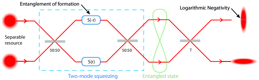
with $\kappa=2(\det\sigma+1)-(m-n)^{2}$ and $\lambda_{\pm}=\det M+\det N-2\det C+2((mn+c^{2})\pm 2c(m+n))$. The meaning of $r_{0}$ is depicted in Fig. 2— it can be identified as the minimum amount of two-mode squeezing that is needed to produce the state $\sigma$, corresponding to an optimal choice of the separable resource. For general two-mode Gaussian states, the expression (Eq. 9 and 10) is a lower bound on the entanglement of formation, and lies relatively close to the exact value Tserkis and Ralph (2017).

The symmetry requirements of Eq. 9 and 10 is, fortunately, not too stringent; for instance, the standard protocols of entanglement swapping Hoelscher-Obermaier and van Loock (2011) and entanglement-based quantum key distribution Cerf et al. (2001) work with entangled resources of this type. However, experimental implementations of these protocols will necessarily be imperfect, which means that quantum states produced in the lab are never perfectly symmetrical. In such cases, numerical methods for calculating the entanglement of formation of arbitrary two-mode Gaussian states can be quite useful Wolf et al. (2004); Adesso and Illuminati (2005); Marian and Marian (2008).

III.4 Logarithmic negativity

For arbitrary density matrices $\hat{\rho}$, the logarithmic negativity $\mathcal{E}_{N}$ is defined to be Vidal and Werner (2002):

$$\mathcal{E}_{N}(\hat{\rho})=\log||\hat{\rho}^{PT}||.$$ (11)

The symbol $||\cdot||$ denotes the trace norm, the notation PT is shorthand for the partial transpose. For two-mode Gaussian states $\sigma$, the logarithmic negativity is a simple function of the symplectic eigenvalue of the partially transposed state $\tilde{\nu}_{-}$:

$$\mathcal{E}_{N}(\sigma)=\begin{cases}0,\text{~{}if $\sigma$ is separable.}\\ -\log\tilde{\nu}_{-},\text{~{}otherwise.}\end{cases}$$ (12)

It is thus a good indicator of inseparability by virtue of the PPT (positive partial transpose) criterion Peres (1996); Horodecki (1997), which states that a Gaussian state is separable if and only if $\tilde{\nu}_{-}\geq 1$ Simon (2000). The logarithmic negativity coincides with the PPT-entanglement cost Audenaert et al. (2003).

While the symplectic diagonalisation of two-mode Gaussian states will lead to uncorrelated thermal states, the symplectic diagonalisation of its partial transpose will lead to squeezing. It is easy to see that the maximum amount of local squeezing one can obtain from a two-mode Gaussian state is given by the symplectic eigenvalue of its partial transpose $\tilde{\nu}_{-}$, and that this can be achieved by interfering the two modes on a beam-splitter (Fig. 2). Although it does not hold in the most general case of Eq. 2, it does hold up to states with the symmetries of Eq. 5. As a consequence of this operational interpretation for $\tilde{\nu}_{-}$, it is related to the entanglement of formation through the following inequality (ref. Adesso and Illuminati (2005), Eq. 43):

$$\tilde{\nu}_{-}\geq e^{-2r_{0}},$$ (13)

which essentially expresses the conservation of squeezing. The equality is attained by symmetric states, but the two measures are in general not equivalent. It has also been conjectured that $e^{-2r_{0}}$ is bounded from below by some non-trivial function of $\tilde{\nu}_{-}$ Adesso and Illuminati (2005), and the gap between the upper and lower bounds would imply that the two measures do not impose the same ordering on quantum states. The disagreement of measures on the ordering of states holds quite generally for the other entanglement measures as well Virmani and Plenio (2000).

III.5 EPR steering

By performing measurements of different observables on one party of an entangled state, it is possible to steer the other party into different types of quantum states Einstein et al. (1935); Schrödinger (1935, 1936). In continuous variable quantum optics, EPR steering can occur when any of the following inequalities on the conditional variances is violated Reid (1989):

$$\mathcal{E}_{A>B}=V_{x_{B}|x_{A}}V_{p_{B}|p_{A}}\geq 1,$$

$$\mathcal{E}_{B>A}=V_{x_{A}|x_{B}}V_{p_{A}|p_{B}}\geq 1.$$

The symbol $V_{x_{A}|x_{B}}$ denotes the conditional variance of the quadrature $\hat{x}_{A}$ given $\hat{x}_{B}$, with the other quantities interpreted in a similar fashion. The subscripts $A$ and $B$ denote two parties sharing a bipartite entangled state. Two inequalities instead of one is necessary for describing steering, because it is a directional quantity. If we assume, without the loss of generality, that entanglement is generated by the party A and distributed to the party B, then we call $\mathcal{E}_{A>B}$ forward steering and $\mathcal{E}_{B>A}$ reverse steering. The party that performs the measurement is the party that performs steering; that would be $A$ in the case of $\mathcal{E}_{A>B}$, and $B$ in the case of $\mathcal{E}_{B>A}$. It is possible for a quantum state to be steerable in one direction, but not in the other. In this case, only one of the inequalities above is violated.

EPR steering is not a measure of entanglement, since it does not characterise the separability of quantum states Bowen et al. (2004); Wiseman et al. (2007); Vedral et al. (1997). It is a sufficient condition for inseparability, but not a necessary condition — there exists quantum states that are entangled but not steerable in either direction. We note that EPR steering has found applications in quantum key distribution — in particular, one-sided device-independent quantum key distribution Branciard et al. (2012); Walk et al. (2016) — where the secure keyrate turned out to be a simple function of EPR steering.

III.6 Relative entropy of entanglement

The quantum relative entropy between any pair of density operators $\hat{\rho}$ and $\hat{\sigma}$ is defined to be

$$S(\hat{\rho}||\hat{\sigma})=tr\hat{\rho}(\log\hat{\rho}-\log\hat{\sigma}).$$ (14)

The relative entropy of entanglement (REE) of $\hat{\rho}$ is then defined by minimising the relative entropy over separable states Vedral et al. (1997):

$$\mathcal{E}_{R}(\hat{\rho})=\inf_{\hat{\sigma}~{}\text{separable}}S(\hat{\rho}||\hat{\sigma}).$$ (15)

By construction, it is zero if and only if $\hat{\rho}$ is separable. The relative entropy of entanglement is an upper bound to the distillable entanglement and a lower bound to the entanglement of formation Vedral and Plenio (1998). One can further specialise the domain of optimisation to Gaussian states, leading to the Gaussian relative entropy of entanglement (GREE) Scheel and Welsch (2001):

$$\mathcal{E}_{GR}(\hat{\rho})=\inf_{\begin{subarray}{c}\hat{\sigma}~{}\text{separable}\\ \hat{\sigma}~{}\text{Gaussian}\end{subarray}}S(\hat{\rho}||\hat{\sigma}).$$ (16)

The separable state which achieves the minimum of Eq. 15 is called the closest separable state, and can be non-Gaussian even if $\hat{\rho}$ is Gaussian Wu et al. (2001); hence, the relative entropy of entanglement and its Gaussian approximation are not equivalent.

One does not have closed expressions for the relative entropy of entanglement in general Friedland and Gour (2011). Although there are numerical methods based on semidefinite programming Zinchenko et al. (2010), this technique is ill-suited in terms of computational time and memory requirements for continuous variable systems; in this paper, we will simply use the Gaussian relative entropy of entanglement as an approximation. We show that the approximation is good in the regime that we care about. Finally, we note that the relative entropy of entanglement has been applied to the study of quantum repeaters; it is an upper limit on the channel capacity, when one does not have access to a quantum repeater Pirandola et al. (2017).

III.7 Squashed entanglement

Squashed entanglement is a measure based on the conditional mutual information Christandl and Winter (2004):

$$\mathcal{E}_{sq}(\hat{\rho}_{AB})=\frac{1}{2}\inf_{\hat{\rho}_{ABE}}I(A:B|E),$$ (17)

where one tries to minimise the conditional mutual information $I(A:B|E)=S(\hat{\rho}_{AE})+S(\hat{\rho}_{BE})-S(\hat{\rho}_{E})-S(\hat{\rho}_{ABE})$ over all purifications $\hat{\rho}_{ABE}$ of the bipartite state $\hat{\rho}_{AB}$. The subscripts $A$, $B$, and $E$ denote the corresponding subsystems similar to that in Eq. 7. The optimisation is difficult to perform, but one can exploit clever choices of the purification to obtain bounds on the squashed entanglement Goodenough et al. (2016). Like the relative entropy of entanglement, squashed entanglement is a bound on the capacities of quantum communication channels; furthermore, it satisfies many axioms of entanglement theory that other measures do not Takeoka et al. (2014).

III.8 Coherent information

The coherent Schumacher and Nielsen (1996) and reverse coherent information Garcia-Patron et al. (2009) are defined as

$$I_{C}(\hat{\rho})=S(tr_{A}\hat{\rho})-S(\hat{\rho}),$$ (18)

$$I_{RC}(\hat{\rho})=S(tr_{B}\hat{\rho})-S(\hat{\rho}),$$ (19)

and, as usual, the $A$ and $B$ subscripts denote subsystems of the bipartite state $\hat{\rho}$. These two measures are not entanglement measures in the axiomatic sense Vedral et al. (1997); however, they satisfy the hashing inequality Devetak and Winter (2005); Pirandola et al. (2017):

$$\max(I_{C}(\hat{\rho}),I_{RC}(\hat{\rho}))\leq\mathcal{E}_{D}(\hat{\rho}),$$ (20)

where $\mathcal{E}_{D}$ denotes the distillable entanglement. By virtue of the hashing inequality, the coherent and reverse coherent information provide sufficient conditions for inseparability, and plays the role of a lower bound in characterising communication channels Pirandola et al. (2017). This is in contrast to the relative entropy of entanglement and squashed entanglement, which would both correspond to upper bounds.

To conclude this section, we emphasise that we have made a choice to work with one particular type of quantum correlation — namely, quantum entanglement. It is a suitable choice for the analysis of entanglement distillation which we present in the next section. Other interesting options include discord measures Ollivier and Zurek (2001), a measure of squeezing Idel et al. (2016), and coherence measures Tan et al. (2017); however, we will not attempt to pursue these directions here.

IV Experiment

IV.1 Entanglement generation and processing

Figure 3: Schematic of the MBNLA experiment Chrzanowski et al. (2014). Squeezed states were generated from a pair of bow-tie cavities using the optical $\chi^{(2)}$ nonlinearity, and combined on a balanced beam-splitter to generate Einstein-Podolsky-Rosen entanglement. One of the beams from the EPR is sent through a communication channel that has optical loss, while the other is sent to a homodyne for verification; the transmission of the channel was characterised by optical heterodyne detection. Post-processing was applied on the data collected from the homodynes to emulate noiseless linear amplification, and thus the distillation of entanglement. H: half-wave plate, Q: quarter-wave plate, PBS: polarising beam-splitter, CW: continuous wave, PPKTP: periodically-poled potassium titanyl phosphate.

We study measurement-based distillation of quantum entanglement using recent advances in entanglement theory. The experiment setup (Fig. 3) consisted of a pair of bow-tie optical parametric amplifiers driven at $532$ nm, with bright squeezed light generated at $1064$ nm. The two beams were combined on a balanced beam-splitter, with a relative phase of $\pi/2$ to give Einstein-Podolsky-Rosen entanglement. One mode of this EPR pair was sent through a communication channel. Under the assumption that the quantum state is Gaussian, we can describe the state using just the first and second moments; five hundred sets of two million optical quadrature measurements were collected from each homodyne detector, retaining the 3-4 MHz narrowband through digital high-pass and low-pass filtering. Measurement-based entanglement distillation was performed using an approach similar to Chrzanowski et al. (2014), by post-processing the homodyne measurement data.

Figure 4: Distribution of an entangled state through channels with various amounts of optical loss. Circles are from experiments, solid lines are theory, and the shaded region above the dashed line correspond to separable states. We include a meter below the figure, which gives the loss-equivalent distance assuming telecom wavelength (i.e. 1550 nm), with the ticks distributed according to a logarithmic scale.

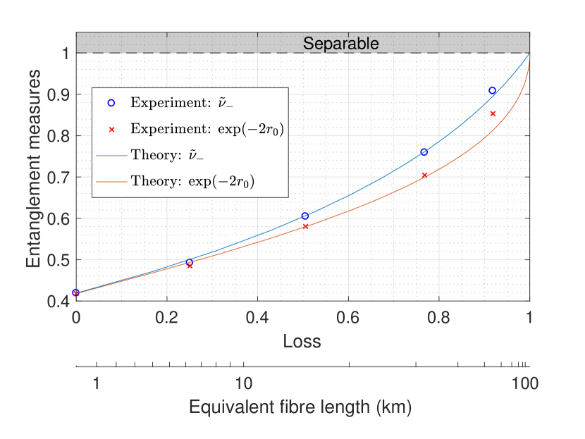
In practice, the communication channel through which we distribute the entanglement will be lossy; here, we will assume that the loss is entirely passive and model it as a beamsplitter with fixed transmissivity. This was implemented using a polarising beam-splitter preceeded by a half-wave plate. As we vary the loss, we can compare the logarithmic negativity and the entanglement of formation using the effective squeezing, which varied according to Fig. 4. We use the term “effective squeezing” of the logarithmic negativity and the entanglement of formation to refer to the quantities $\tilde{\nu}_{-}$ and $\exp(-2r_{0})$, respectively. These quantities characterise the respective measures, and, at the same time, can be interpreted as quantum squeezing (sections III.3 and III.4.) At unity transmissivity (no loss), the state is symmetric but mixed, due to decoherence in the entanglement generation process. Despite the mixture, the measures remain equivalent due to the symmetry. In the presence of loss, the states are asymmetric and the measures are no longer equal. This is with the exception of maximal loss (zero transmissivity), where nothing is transmitted and the state is separable. All measures register effectively no squeezing in this case, which corresponds to unity when expressed as a variance.

The effects of passive loss can be mitigated through the use of noiseless linear amplification (NLA) Ralph and Lund (2009); Fiurasek (2009). This peculiar amplifier can be described by an unbounded operator $g^{\hat{n}}$, where $g$ represents the amplitude gain. Acting the noiseless linear amplifier on a coherent state will amplify the complex amplitude without increasing the noise, while acting it on a continuous variable EPR state with loss would lead to a state with increased squeezing and reduced loss Ralph and Lund (2009). Due to the unbounded nature of the NLA operator, implementations are necessarily approximate; in order to avoid violating the Heisenberg uncertainty principle, they must also be non-deterministic Caves (1982). Experimental implementations of the NLA are subject to additional limitations, such as restrictions on the size of the input coherent amplitudes to small values Xiang et al. (2010).

In this paper, a virtual implementation of the noiseless linear amplifier Chrzanowski et al. (2014) has been chosen due to the ease of implementation. An NLA followed by optical heterodyning is equivalent to heterodyning followed by data processing; thus one is able to implement the noiseless linear amplifier in the form of data processing, provided that one performs a heterodyne measurement. Concretely, one takes each outcome $\alpha$ of the heterodyne and postselects it with an acceptance probability given by Fiurasek and Cerf (2012):

$$P(\alpha)=\begin{cases}e^{(1-1/g^{2})(|a|^{2}-|\alpha_{c}|^{2})},|\alpha|\leq|\alpha_{c}|.\\ 1,|\alpha|>|\alpha_{c}|.\end{cases}$$ (21)

where $g$ corresponds to the amplitude gain, and $\alpha_{c}$ is a constant which specifies a cutoff. One then scales the successful events by multiplication: $\alpha\mapsto\alpha/g$. The postselection and rescaling make up the data-processing stage which emulates the noiseless linear amplifier. The closeness by which this measurement-based implementation approximates the true NLA depends on the cutoff — a larger cutoff will improve the approximation at the expense of a smaller probability of success Zhao et al. (2017).

IV.2 Experiment analysis

(a)

(b)

Figure 5: Entanglement measures as a function of the probability of success. The optical loss was set to $90\%$. Circles correspond to experiment data, solid lines to theory calculations, dashed lines to the (measure-dependent) deterministic bound, and error bars represent 1.5 standard deviations over 100 repeated runs of postselection. The theory line can be calculated straightforwardly, assuming that the state is Gaussian (fitted to the measured covariance matrix) and that the postselection filter is ideal (i.e. infinite cutoff). The data points show positive bias relative to the theory model, which correspond to deviations from normality due to experimental imperfections and to the non-ideal filter implementation (Eq. 21). (a) Both measures increase with decreasing probability of success, but only logarithmic negativity surpassed the deterministic bound. (b) All of the measures in this figure lie below their respective deterministic bounds. The distillable entanglement is bounded from above by the relative entropy of entanglement, and this is represented by the orange region; in the case of the deterministic bound, the two measures coincide (represented by the overlaying orange and rose-coloured dashed lines).

Figure 6: Demonstrating an increase in the distillable entanglement. The loss was set to $0\%$. The distillable entanglement is bounded from above and from below by the relative entropy of entanglement and the reverse coherent information, respectively. The boundary between the orange and blue regions is a horizontal line corresponding to the relative entropy of entanglement at unity probability of success, and values of the reverse coherent information lying in the orange region imply an increase in the distillable entanglement. The theory lines (given by the solid lines) in this figure assumes a finite cutoff, with the case of infinite cutoff also calculated for the reverse coherent information, showing that its values are smaller but remains in the orange region at small probabilities of success.

The results of the analysis is presented in Figs. 5, 6, and 8. We considered three different settings of loss — $90\%$ (Fig. 5a, 5b, and 8a), $50\%$ (Fig. 8b and 8c), and $0\%$ (Fig. 6). For each loss, the maximum gain $g$ for the postselection filter was set to $1.6$, $1.4$, and $1.28$ respectively, with unity gain corresponding to no postselection. We make the Gaussian assumption, and infer the effective quantum state conditioned on successful postselection by calculating the covariance matrix of the post-processed data. The cutoff for the filter was chosen to be large enough to justify the Gaussian assumption to at least $95\%$ using the Jarque-Bera test of normality, which is based on skewness and kurtosis (the third and fourth moments). The entanglement measures may finally be evaluated on these effective states. We remark that different values of loss played different roles — a large amount of loss ($90\%$) draws a clear distinction between logarithmic negativity and the other entanglement measures; a moderate amount of loss ($50\%$) highlights the directionality of EPR steering and of coherent information; and a minimal amount of loss ($0\%$) allows us to certify an increase in the distillable entanglement.

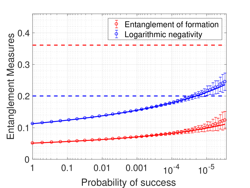
In Fig. 5 and 8, all measures indicate increasing entanglement with decreasing probability of success, as they should. What is perhaps more interesting is a comparison with the deterministic bound — that is, the maximum entanglement that can be transmitted through the channel in a deterministic fashion using an EPR resource with infinite squeezing. The resulting state is known as the Choi state of the channel Choi (1975). We note that the deterministic bound is measure-dependent, corresponding to the values of each measure evaluated on the Choi state. In Fig. 5a, we see that logarithmic negativity crosses its deterministic bound at a relatively large probability of success, whereas the other measures will also cross their respective bounds but at much lower probabilities. The entanglement of formation was particularly far away from the bound even at the small success probability of $10^{-6}$, although it can in principle cross the bound at sufficiently low probabilities of success Tserkis et al. (2018). We attribute this discrepancy to the operational meanings of the measures. The entanglement of formation measures the squeezing operations needed to produce an entangled state, while the logarithmic negativity is related to local squeezing that can be extracted from the state. The deterministic bound corresponds to a state for which a lot of squeezing is needed to produce it, but not much can be extracted from it; thus possessing a large entanglement of formation, but a lower logarithmic negativity.

Figure 7: A comparison of the relative entropy of entanglement and its Gaussian approximation. Inset shows the convergence of the numerical optimisation for the relative entropy of entanglement as a function of the photon number cutoff; the cutoff is necessary as we are approximating a continuous variable system using a finite-dimensional density matrix. The loss was set to $90\%$, and in such a case we find the two measures to be almost indistinguishable.

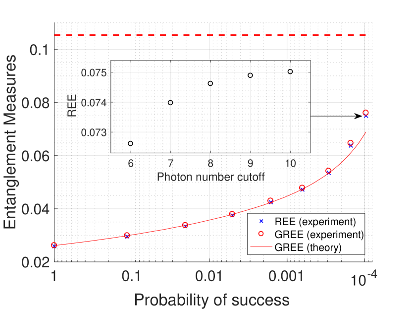
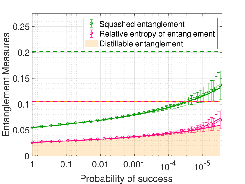
Results for the relative entropy of entanglement, for the squashed entanglement, and for the distillable entanglement are shown in Fig. 5b. We approximate the relative entropy of entanglement using its Gaussian version (as explained in Section III.6), numerically performing the minimisation of Eq. 16 over separable two-mode Gaussian states. This approximation works relatively well when there is a large amount of loss (Fig. 7). Finally, the deterministic bound can be calculated analytically Pirandola et al. (2017), and one finds that the relative entropy of entanglement does not cross the deterministic bound. We emphasise that the effects of noiseless linear amplification — the increase in squeezing and the reduction of loss Ralph and Lund (2009) — guarantees that any measure must cross the bound at sufficiently small probabilities of success. However, the value of the probability of success might be too small to be accessed in the experiment, which is the case here.

Another important point to note for Fig. 5b is that the deterministic bound for the relative entropy of entanglement coincides with the bound for the distillable entanglement Pirandola et al. (2017). This is a useful fact for showing that the distillable entanglement does not cross the bound either. Although we cannot calculate the distillable entanglement directly (for general states other than the Choi state), we can bound it from above using the relative entropy of entanglement, as illustrated by the orange shaded region in Fig. 5b. This region lies below the deterministic bound, thus demonstrating that the distillable entanglement does not cross the bound.

We stress that the logarithmic negativity and the entanglement of formation are unable to provide evidence of this, despite being upper bounds of the distillable entanglement like the relative entropy of entanglement is. Both measures cross the deterministic bound that is given by the distillable entanglement, which one can read off Fig. 5b to be approximately 0.1 in value; thus these measures are unable to rule out the possibility that the distillable entanglement could have crossed the deterministic bound. As we have discussed in the previous paragraph, this cannot be true because the distillable entanglement is always lesser than the relative entropy of entanglement, which is in turn lesser than the deterministic bound of the distillable entanglement. The conclusion that the distillable entanglement did not cross the deterministic bound can only be drawn using the relative entropy of entanglement as the upper bound.

Fig. 5b also shows results for squashed entanglement. Squashed entanglement is one of the measures for which there exist no convenient methods for calculating it; at best, we have a handful of bounds. For the case of two-mode Gaussian states, one of the best known bounds is given in Goodenough et al. (2016); it can be evaluated for arbitrary phase-insensitive Gaussian channels, and hence for states of the form Eq. 5, but not for those in the general form of Eq. 2. We note that such a requirement can be addressed by simply averaging the correlations of the amplitude and the phase quadratures, which are sufficiently close for the two-mode squeezed state generated in this experiment. As shown in Fig. 5b, squashed entanglement does not cross the bound; however, one should keep in mind that the values for the squashed entanglement are approximations in the form of an upper bound, and not the actual value of the measure itself.

We pause briefly to discuss the significance of the collective results in Fig. 5. The crossing of the deterministic bound by the logarithmic negativity suggests that the distilled state is better than the Choi state (i.e. an EPR state with infinite squeezing transmitted through the same communication channel). The possibility of doing better than the Choi state is certainly not forbidden by the laws of quantum mechanics, and can, for instance, be achieved by using the noiseless linear amplifier with very large gains Ralph and Lund (2009). Nonetheless, we found that the logarithmic negativity has apparently “jumped the gun” — it suggests that this has already been achieved in the present experiment when all the other measures indicate otherwise. Thus, we have demonstrated a drawback for using the logarithmic negativity as the figure of merit, which is perhaps the price that one has to pay since it can be calculated so trivially.

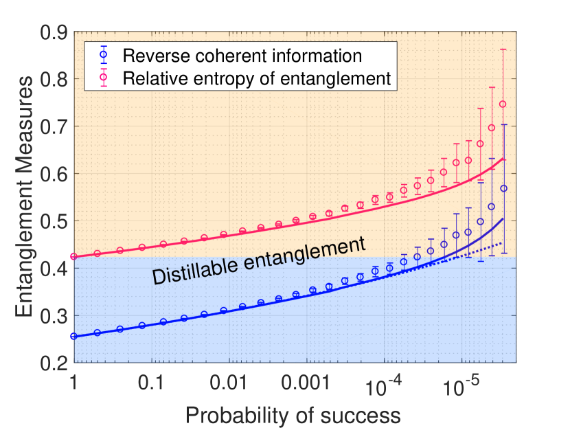
Returning to the analysis, we consider the distillable entanglement in Fig. 6. It is similar to squashed entanglement in the sense that neither can be evaluated using straightforward means, but they differ because some of the bounds on the distillable entanglement are rather stringent Pirandola et al. (2017). We employ these stringent upper and lower bounds on the distillable entanglement to demonstrate an increase in this quantity in the case of the lossless channel. We note that such a task would have been trivial if we knew how to calculate the measure — the need for using bounds in the case of the distillable entanglement is precisely because there is no method for calculating it directly.

Similar to Ref. Dong et al. (2010, 2008), we use the reverse coherent information to bound the distillable entanglement from below; however, we use the relative entropy of entanglement instead to bound it from above (as opposed to using the logarithmic negativity in Ref. Dong et al. (2010, 2008)). If, after performing the entanglement distillation, the reverse coherent information ends up greater than the relative entropy of entanglement that we had started off with (indicated by the orange shading in Fig. 6), one may conclude that the distillable entanglement has increased. If the reverse coherent information remains smaller, then no conclusion can be drawn (corresponding to the blue shading). Fig. 6 shows values of the reverse coherent information surpassing the bound given by the relative entropy of entanglement at low probabilities of success, and hence an increase in the distillable entanglement. We remark that these results are fundamentally limited by state preparation and measurements — it cannot be improved simply by adjusting the postselection settings, due to excess noise and to the diminishing probability of success. In addition, the upper bound and the channel transmissivity cannot be arbitrary. There are other choices for the upper bound (Sec. III.2), and one can also consider other settings for the loss (anything between $0\%$ and $100\%$); however, no increase in the distillable entanglement was observed in any of these cases using the method presented above. In this sense, the results in Fig. 6 is optimal.

(a)

(b)

(c)

Figure 8: Relatives of entanglement measures. The loss in a was set to $90\%$, while that in b and c is $50\%$. The data points, theory lines, deterministic bounds, and the error bars should be interpreted in the same way as those for Fig. 5. Noiseless linear amplification is useful for recovering forward steering and coherent information, but less so for the other direction which is more robust to loss.

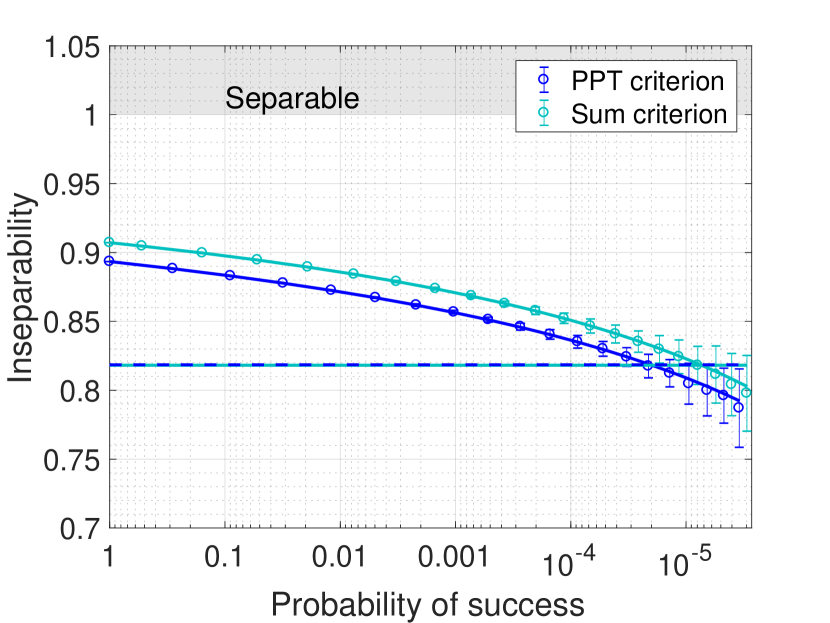
Adding to the collection, we consider relatives of entanglement measures. These are not proper entanglement measures in the axiomatic sense. Fig. 8a illustrates the inseparability criteria for two-mode Gaussian states; the sum criterion Duan et al. (2000) displays similar behavior to the PPT criterion, as both measures deal with the extraction of squeezing from entangled states Giovannetti et al. (2003). The sum criterion relies on an extraction protocol that is suboptimal compared to the PPT criterion, hence its values are closer to the separable boundary. Both are, of course, equally valid for certifying inseparability.

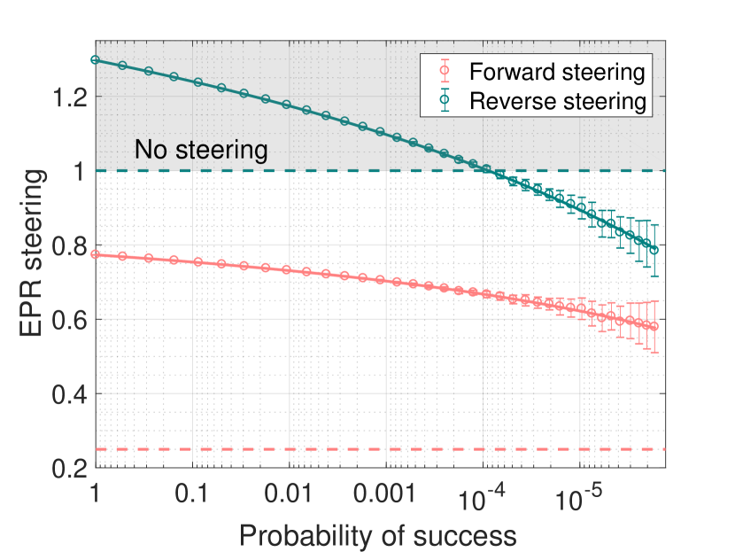
In Fig. 8b we show the results for EPR steering, a directional quantity for which the properties depend on the direction of interest. Reverse steering is particularly succeptible to loss, where an entangled state transmitted through $50\%$ of loss would not be steerable in the reverse direction. It is interesting to note that, for this particular case, violation of the EPR steering criterion is equivalent to surpassing the deterministic bound. This is not true in general. By performing noiseless linear amplification, one is able to recover reverse steering beyond the deterministic bound at reasonable success probabilities, and one may compare this with forward steering — the deterministic bound is smaller to begin with, and is also much harder to beat. Reverse steering is sensitive to loss because one is trying to steer using the lossy mode — most of the information about the entangled state has already been lost to the environment. In the case of direct steering, there is an advantage since one is using the mode that does not suffer from the loss of the channel.

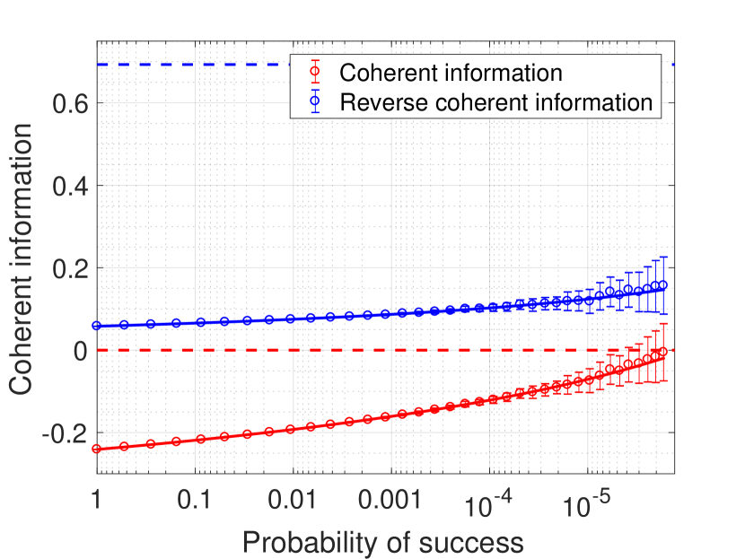
Finally, we consider the coherent information and the reverse coherent information, which are related to entanglement through the hashing inequality (Eq. 20). The reverse coherent information is robust against loss for the same reason that direct steering is; likewise, the coherent information is fragile the same way reverse steering is succeptible to loss (Fig. 8c). The reverse coherent information is always positive even when no noiseless linear amplification was performed, while the coherent information was not initially positive but could be recovered at some small probability of success that is just out of reach in this experiment. Due to the robustness of the reverse coherent information, the deterministic bound is much harder to surpass.

V Conclusion

By analysing a measurement-based entanglement distillation experiment using a collection of measures, we showed that the logarithmic negativity exhibits behavior quite distinct from the others. It would make us believe that more entanglement has been distilled than what is offered by the deterministic bound, in stark contrast to what the other measures suggest. In addition to this result, we were also able to certify an increase in the distillable entanglement (in the case of the lossless channel), relying primarily on a judicious choice of the upper bound in order to estimate this quantity accurately. The work we have presented is useful for analysing entanglement distillation, but can also be extended to more general situations; this includes entanglement swapping, for instance, and the analysis of quantum repeaters in general.