Uncertainty-aware Audiovisual Activity Recognition using Deep Bayesian Variational Inference

Abstract

Deep neural networks (DNNs) provide state-of-the-art results for a multitude of applications, but the approaches using DNNs for multimodal audiovisual applications do not consider predictive uncertainty associated with individual modalities. Bayesian deep learning methods provide principled confidence and quantify predictive uncertainty. Our contribution in this work is to propose an uncertainty aware multimodal Bayesian fusion framework for activity recognition. We demonstrate a novel approach that combines deterministic and variational layers to scale Bayesian DNNs to deeper architectures. Our experiments using in- and out-of-distribution samples selected from a subset of Moments-in-Time (MiT) dataset show a more reliable confidence measure as compared to the non-Bayesian baseline and the Monte Carlo dropout (MC dropout) approximate Bayesian inference. We also demonstrate the uncertainty estimates obtained from the proposed framework can identify out-of-distribution data on the UCF101 and MiT datasets. In the multimodal setting, the proposed framework improved precision-recall AUC by 10.2% on the subset of MiT dataset as compared to non-Bayesian baseline.

1 Introduction

Vision and audio are complementary inputs and fusing these modalities can greatly benefit an activity recognition application. Multimodal audiovisual activity recognition using deep neural network (DNN) architectures are not successful in modeling the inherent ambiguity in the correlation between two modalities. One of the modalities (e.g., sneezing in audio, writing in vision) can be more certain about the activity class than the other modality. It is important to model reliable uncertainty estimates for the individual modalities to benefit from multimodal fusion.

DNNs trained on large datasets [23, 1, 30] have been successful in solving many perception tasks with state-of-the-art results. However, DNNs are trained to obtain the maximum likelihood estimates and disregard uncertainty around the model parameters that eventually can lead to predictive uncertainty. Deep learning models may fail in the case of noisy or out-of-distribution data, leading to overconfident decisions that could be erroneous as softmax probability does not capture overall model confidence. Instead, it represents relative probability that an input is from a particular class compared to the other classes.

Probabilistic Bayesian models provide principled ways to gain insight about data and capture reliable uncertainty estimates in predictions. Bayesian deep learning [32, 12] has allowed bridging DNNs and probabilistic Bayesian theory to leverage the strengths of both methodologies. Bayesian deep learning framework with Monte Carlo (MC) dropout approximate inference [13] is used in visual scene understanding applications including camera relocalization [25], semantic segmentation [24] and depth regression [26].

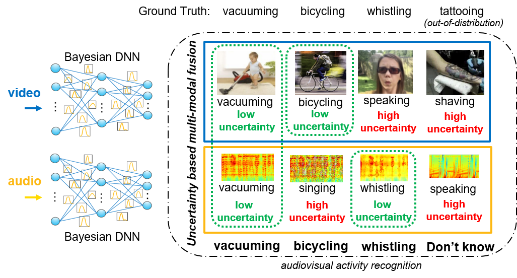
Figure 1: Uncertainty-aware audiovisual activity recognition

Activity recognition is an active area of research with multiple approaches depending on the application domain and the types of sensors [28]. Human activity recognition using wearable sensors such as accelerometer/gyroscopes and heart-rate monitors is used to recognize everyday human activities that include walking, running, and swimming. Human pose-based activity recognition [37, 40] methods aggregate motion and appearance information along tracks of human body parts to recognize human activity. Multimodal methods which combine optical flow or depth information along with RGB data [41, 39] are shown to provide state-of-the-art results for generic (not just human) activity recognition tasks. Methods which combine semantic level information [53] such as pose, object/scene context and other attributes including linguistic descriptors have been proposed to detect group activities.

In this work, we focus on audiovisual activity recognition and use Bayesian DNN with stochastic variational inference (VI) to reliably estimate uncertainty associated with the individual modalities for multimodal fusion (as shown in Figure 1).

Our main contributions in this work include:

1. A multimodal fusion framework based on predictive uncertainty estimates applied to activity recognition: To the best of our knowledge, this is the first work on multimodal fusion based on uncertainty estimates using Bayesian deep learning with variational inference.

2. A scalable variational inference with hybrid Bayesian DNN architecture by combining deterministic and variational layers.

3. Identifying out-of-distribution data for audiovisual activity recognition using uncertainty estimates: We demonstrate the uncertainty estimates obtained from the proposed architecture can identify out-of-distribution data in Moments-in-Time (MiT) and UCF-101 action recognition datasets.

The rest of the document is divided into the following sections. The background on Bayesian DNNs and audiovisual activity recognition are presented in Section 2. In Section 3, the proposed Bayesian multimodal DNN architecture is presented. The results are presented in Section 4, followed by conclusions in Section 5.

2 Background

2.1 Bayesian deep neural networks

Bayesian DNNs provide a probabilistic interpretation of deep learning models by placing distributions over the model parameters (shown in Figure 2). Bayesian inference can be applied to estimate the predictive distribution by propagating over the model likelihood while marginalizing over the learned posterior parameter distribution. Bayesian DNNs also help in regularization by introducing distribution over network parameters, capturing the posterior uncertainty around the neural network parameters. This allows transferring inherent DNN uncertainty from the parameter space to the predictive uncertainty.

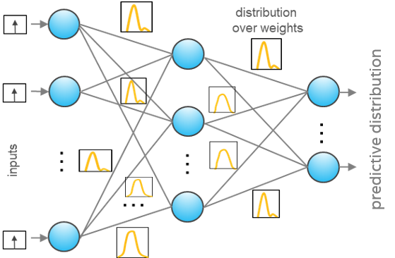
Figure 2: Bayesian neural network

Given training dataset $D=\{x,y\}$ with inputs $x={x_{1},...,x_{N}}$ and their corresponding outputs $y={y_{1},...,y_{N}}$, in parametric Bayesian setting we would like to infer a distribution over parameters $w$ as a function $y=f_{w}(x)$ that represents the DNN model. With the posterior for model parameters inferred during Bayesian neural network training, we can predict the output for a new data point by propagating over the model likelihood $p(y|x,w)$ while drawing samples from the learned parameter posterior $p(w|D$). Equation 1 shows the posterior distribution of model parameters obtained from model likelihood.

$$p(w|D)=\frac{p(y|x,w)p(w)}{p(y|x)}$$ (1)

Computing the posterior distribution $p(w|D)$ is often intractable, some of the previously proposed techniques to achieve an analytically tractable inference include: (i) Markov Chain Monte Carlo (MCMC) sampling based probabilistic inference [32, 47] (ii) variational inference techniques to infer the tractable approximate posterior distribution around model parameters [17, 36, 7] and (iii) Monte Carlo dropout approximate inference [13].

Variational inference [22, 6] is an active area of research in Bayesian deep learning, which uses gradient based optimization. This technique approximates a complex probability distribution $p(w|D)$ with a simpler distribution $q_{\theta}(w)$, parameterized by variational parameters $\theta$ while minimizing the Kullback-Leibler (KL) divergence [5]. Minimizing the KL divergence is equivalent to maximizing the log evidence lower bound [5, 13].

$$\mathcal{L}:=\int q_{\theta}(w)\,log\,p(y|x,w)\,dw$$ (2)

$$~{}~{}~{}~{}~{}~{}~{}~{}~{}~{}~{}~{}~{}~{}~{}~{}~{}~{}~{}~{}-KL[q_{\theta}(w)||p(w)]$$

Predictive distribution is obtained through multiple stochastic forward passes through the network during the prediction phase while sampling from the posterior distribution of network parameters through Monte Carlo estimators. Equation 3 shows the predictive distribution of the output $y^{*}$ given new input $x^{*}$:

$$\begin{gathered}p(y^{*}|x^{*},D)=\int p(y^{*}|x^{*},w)\,q_{\theta}(w)dw\\ p(y^{*}|x^{*},D)\approx\frac{1}{T}\sum_{i=1}^{T}p(y^{*}|x^{*},w_{i})~{},~{}~{}~{}w_{i}\sim q_{\theta}(w)\end{gathered}$$ (3)

where, $T$ is number of Monte Carlo samples.

In [12, 26], modeling aleatoric and epistemic uncertainty is described. We evaluate the epistemic uncertainty using Bayesian active learning by disagreement (BALD) [21] for the activity recognition task. BALD quantifies mutual information between parameter posterior distribution and predictive distribution, as shown in Equation 4.

$$BALD:=H(y^{*}|x^{*},D)-\operatorname{\mathbb{E}}_{p(w|D)}[H(y^{*}|x^{*},w)]\\$$ (4)

where, $H(y^{*}|x^{*},D)$ is the predictive entropy which captures a combination of aleatoric and epistemic uncertainty given by:

$$H(y^{*}|x^{*},D)=-\sum_{i=0}^{K-1}p_{i\mu}\,log\,p_{i\mu}\\$$ (5)

$p_{i\mu}$ is predictive mean probability of $i^{th}$ class from $T$ Monte Carlo samples and K is the total number of output classes.

2.2 Audiovisual Activity Recognition

Vision and audio are the ubiquitous sensor inputs which are complementary in nature and have different representations. Audiovisual methods apply joint modeling of the audio and vision inputs [33, 2] to achieve higher accuracies for complex tasks such as activity recognition.

Multimodal models are proposed for audiovisual analysis tasks such as emotion recognition [42], audiovisual speech recognition [33], speech localization [14, 34], cross-modal retrieval [4]. The audiovisual speech recognition (AVSR) task is shown to benefit from multimodal training of the joint models. In [33], a deep autoencoder model for cross-modality feature learning is proposed, where better features for one modality can be learned if multiple modalities are present at training time. A deep audio-visual speech recognition model [2] using self-attention encoder architecture is proposed to recognize speech from talking faces using vision and audio inputs. Recent work on sound localization and separation [14, 34] has shown the benefits of a joint audiovisual representation for cross-modal self-supervised learning using only audio-visual correspondence as the objective function. These audiovisual methods apply joint modeling of the audio and vision inputs during the training phase for better generalizability of the models, but then use single modality during the inference phase. None of the methods listed here provide a quantifiable means to determine the relative importance of each modality.

Vision-based activity recognition techniques apply a combination of spatiotemporal models [45, 3, 51] to capture pixel-level information and temporal dynamics of the scene. In recent years, visual activity recognition models often use ConvNets-based models for spatial feature extraction. The image-based models [19, 43] are pre-trained on ImageNet dataset to represent the spatial features. The temporal dynamics for activity recognition [46, 52] is typically modeled either by using a separate temporal sequence modeling such as variants of RNNs [10, 49] or by applying 3D ConvNets [9], which extend 2D ConvNets to the temporal dimension. Bayesian neural network is used for visual activity recognition [27] to capture uncertainty estimates.

Following the successes of ConvNets on vision tasks, they are shown to provide state-of-the-art results for audio classification as well. Many of the top performing methods from recent audio classification challenges [29, 35] use DNN architectures [38, 11, 50] with convolutional layers. In [20], a model similar to the VGG architecture (VGGish model) from the vision domain was trained using log-Mel spectrogram features on the Audio Set [15] dataset. Audio Set contains over one million Youtube video samples labeled with a vocabulary of acoustic events.

In this work, we focus on audiovisual activity recognition using Bayesian DNNs on the trimmed video samples. The 3D-ConvNet (C3D) architecture [44] is shown to provide generic spatiotemporal representation for multiple vision tasks. We use a variant of 3D-ConvNet ResNet-101 C3D [18] architecture for the visual representation. We use VGGish architecture [20] for audio representation, which is shown to provide generic features for audio classification tasks.

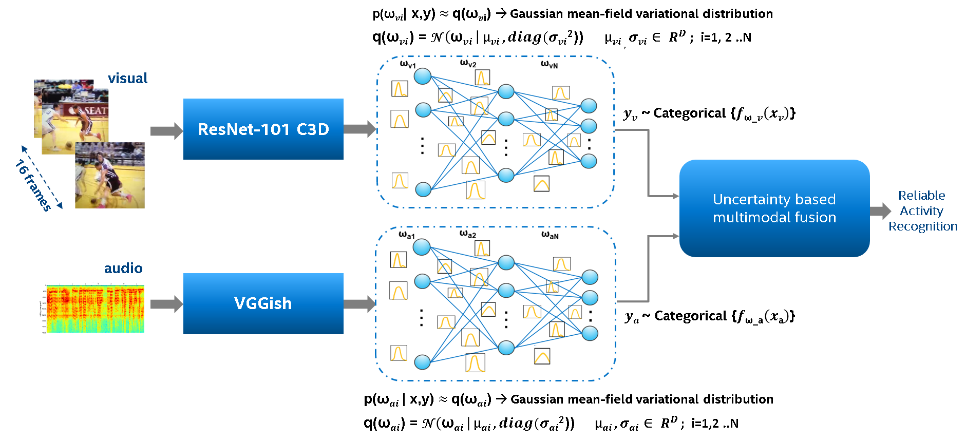
Figure 3: Bayesian audiovisual activity recognition: ResNet-101 C3D and VGGish DNN architectures are used to represent vision and audio information, respectively. The final layer of the DNN is replaced with three fully connected variational layers followed by categorical distribution. The Bayesian inference is applied to the variational layers through Monte Carlo sampling on the posterior of model parameters, which provides the predictive distribution.

3 Bayesian Multimodal DNN Architecture

We present a Bayesian multimodal fusion framework based on uncertainty estimates for audiovisual activity recognition. The block diagram of the proposed audiovisual activity recognition using Bayesian variational inference is shown in Figure 3. We use the ResNet-101 C3D and VGGish architectures for visual and audio modalities, respectively. We replace the final fully connected layer for both vision and audio DNN models with three fully connected variational layers followed by the categorical distribution.

The weights in fully connected variational layers are modeled through mean-field Gaussian distribution, and the network is trained using Bayesian variational inference based on KL divergence [36, 7]. In order to learn the posterior distribution of model parameters $w$, we train Bayesian DNN with variational inference method. The objective is to optimize log evidence lower bound (ELBO) (Equation 2) as the cost function. The model parameters of the fully connected variational layers are parametrized by mean $\mu$ and variance $\sigma^{2}$, i.e. $q_{\theta}(w)=\mathcal{N}(w|\mu,\sigma^{2})$. These parameters in the variational layers are optimized by minimizing the negative ELBO loss ($L^{v}$) [5]:

$$L^{v}=-\mathbb{E}_{q_{\theta}(w)}[log\,p(y|x,w)]+KL[q_{\theta}(w)||p(w)]$$ (6)

$~{}~{}~{}~{}~{}~{}~{}\mu_{i+1}\leftarrow\mu_{i}-\alpha\,\Delta_{\mu}L^{v}_{i}~{}~{}~{}\,\,\,\,\,\,\,\,\,\,\,\,\sigma_{i+1}\leftarrow\sigma_{i}-\alpha\,\Delta_{\sigma}L^{v}_{i}\\ \\$ where, $i$ is the training step, $\alpha$ is the learning rate, $\Delta_{\mu}L^{v}$ and $\Delta_{\sigma}L^{v}$ are gradients of the loss function computed w.r.t $\mu$ and $\sigma$, respectively. We use Flipout [48], which is an efficient method that decorrelates the gradients within a mini-batch by implicitly sampling pseudo-independent weight perturbations for each input.

The parameters in deterministic layers are optimized using cross-entropy loss ($L^{d}$) [16] given by:

$$L^{d}=-\sum_{c}\,y_{c}\log\,\hat{y_{c}}$$ (7)

where, $y_{c}$ and $\hat{y_{c}}$ are true and predicted label distributions, respectively. The model parameters for variational and deterministic DNN layers are obtained by applying stochastic gradient descent optimizer [8] to the loss functions given in Equation 6 and 7, respectively. During prediction stage we perform multiple Monte Carlo forward passes on the final variational layers by sampling the parameters from learned posteriors to measure uncertainty estimates using Equation 4 & 5.

Figure 4 shows accuracy vs uncertainty confusion matrix (proposed in [31] for semantic segmentation), which includes number of accurate and certain ($n_{ac}$), inaccurate and uncertain ($n_{iu}$), accurate and uncertain ($n_{au}$), inaccurate and certain($n_{ic}$) predictions. Equation 8 provides an accuracy vs uncertainty ($A\text{v}U$) metric obtained from the confusion matrix values.

$$A\text{v}U=\frac{n_{ac}+n_{iu}}{n_{ac}+n_{au}+n_{ic}+n_{iu}}$$ (8)

A reliable model will provide higher $A\text{v}U$ score. An uncertainty threshold value that maximizes $A\text{v}U$ metric from individual modalities is the optimal threshold, which is used for multimodal fusion (shown in Figure 5). We perform average pooling of the audio-vision predictive distributions if the uncertainty measures are below the optimal threshold values, else we rely on the single modality that has lower uncertainty measure.

Figure 4: Accuracy vs Uncertainty confusion matrix

For comparison with the non-Bayesian baseline, we maintain the same model depth as the Bayesian DNN model and use three deterministic fully connected final layers for the non-Bayesian DNN model. The dropout is used after every fully connected layer to avoid over-fitting of the model. In the rest of the document, we refer the non-Bayesian DNN model as simply the DNN model. In the following section, we present the results from our experiments showing the effectiveness of Bayesian DNN over conventional DNN models.

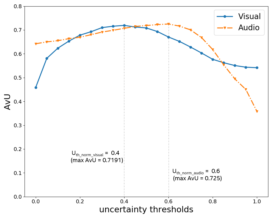
Figure 5: Accuracy vs Uncertainty plots for vision and audio modality. The peak $A\text{v}U$ values represent optimal uncertainty threshold values.

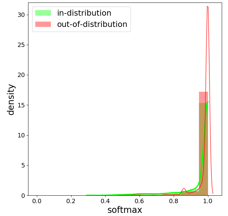
(a) DNN
confidence measure

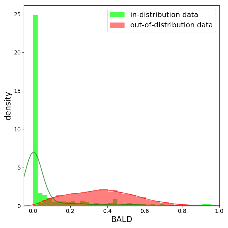
(b) Bayesian DNN (MC Dropout) uncertainty measure

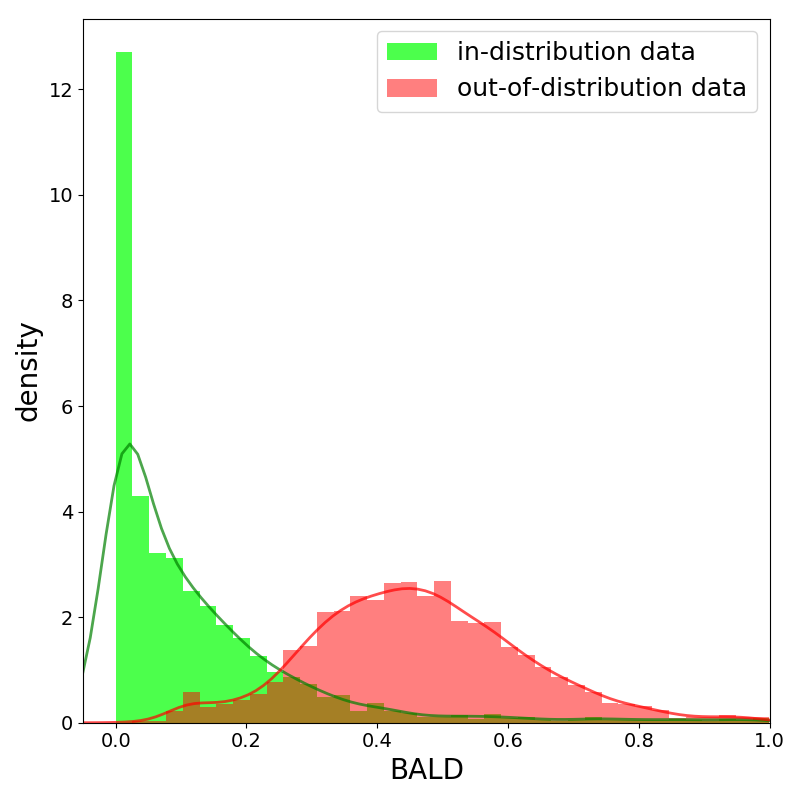
(c) Bayesian DNN (Stochastic VI) uncertainty measure

Figure 6: Density histograms obtained from in- and out-of-distribution samples for the subset of MiT dataset. (a) DNN confidence measure, (b) Bayesian DNN ()MC Dropout) uncertainty measure and (c) Bayesian DNN (Stochastic VI) uncertainty measure. DNN model indicates high confidence for both the categories(peaked to the right or higher values). Bayesian DNN model uncertainty estimates indicate higher uncertainty for out-of-distribution samples as compared to the in-distribution samples. [The density histogram is a histogram with area normalized to one. Plots are overlaid with kernel density curves for better readability.]

4 Results

We analyze the model performance on the Moments-in-Time (MiT) [30] dataset. The MiT dataset consists of 339 classes, and each video clip is 3 secs (~90 frames) in length. In this work, we considered a subset of 54 classes as in-distribution and another 54 classes as out of distribution samples. The selected dataset for both the categories include audio information. In order to check whether DNNs can provide a reliable confidence measure, the subset of 54 classes for each category are selected after subjective evaluation to confirm the activities fall into two distinct distribution of classes. This will allow the comparison of confidence measures between DNN and Bayesian DNN models for in- and out-of-distribution classes, and the uncertainty estimates for the Bayesian DNN models (as the DNN model does not provide uncertainty estimates).

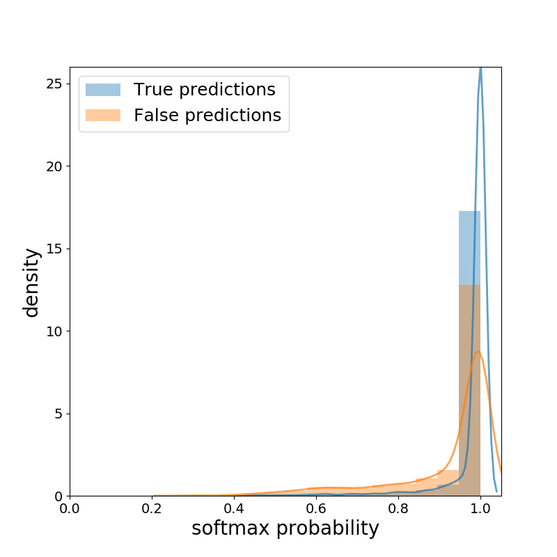
(a) DNN model

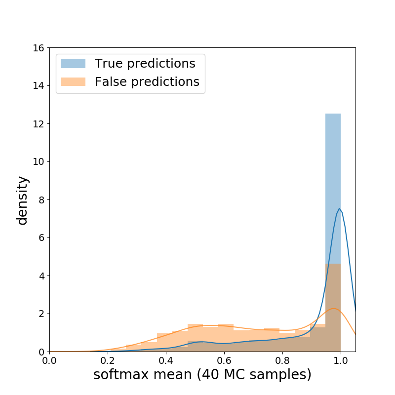
(b) Bayesian DNN (MC Dropout) model

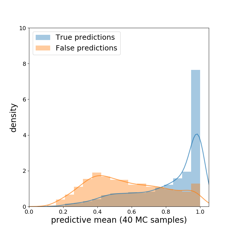
(c) Bayesian DNN (Stochastic VI) model

Figure 7: Density histogram of confidence measures for subset of MiT dataset in-distribution true (correct) and false (incorrect) predictions: A distribution skewed towards right (near 1.0 on x-axis) indicates the model has higher confidence in predictions than the distribution skewed towards left. DNN model indicates high confidence for both true and false predictions. Bayesian DNN model shows lower confidence for false predictions while maintaining higher confidence values for the true predictions. [The density histogram is a histogram with area normalized to one. Plots are overlaid with kernel density curves for better readability.]

The ResNet-101 C3D DNN model is initialized with pretrained weights for the Kinetics dataset [23]. We optimize the model for MiT dataset with transfer learning by training the final fourteen layers. The VGGish model is initialized with pretrained weights for the Audio set [15] dataset. We optimize the model for MiT dataset with transfer learning by training the final five layers. We used stochastic gradient descent (SGD) optimizer with an initial learning rate of 0.0001 and momentum factor of 0.9 along with rate decay when the loss is plateaued.

We trained the ResNet101-C3D vision and VGGish audio architectures using the in-distribution MiT dataset, which includes ~150K training and ~5.3K validation samples. We select individual vision and audio paths from the model shown in Figure 3 to obtain single modality results. In the case of Bayesian DNN stochastic VI model, we perform multiple stochastic forward passes on the final three fully connected variational layers with Monte Carlo sampling on the weight posterior distributions. In our experiments, 40 forward passes provide reliable estimates above which the final results are not affected. Bayesian DNN model predictive mean is obtained by averaging the confidence estimates from the Monte Carlo sampling predictive distributions.

Bayesian active learning by disagreement (BALD) and predictive entropy uncertainty estimates for Bayesian DNN model are obtained using Equation 4 and 5. Figure 5 shows the accuracy vs uncertainty ($A\text{v}U$) metric plots for audio and vision modalities. An optimal threshold for uncertainty measure that will maximize the $A\text{v}U$ score is computed. For the audiovisual Bayesian DNN results, we perform average pooling of the audio-vision predictive distributions if the uncertainty measures are below the optimal threshold values ($U_{th\_visual}$ and $U_{th\_audio}$), else we fall back to the single modality with lower uncertainty measure. In the case of audiovisual DNN model, average pooling of the softmax confidence values from the two modalities is used.

We compare the proposed stochastic VI Bayesian DNN with the baseline DNN model. We also compare with well-known Monte Carlo (MC) dropout [13] approximate Bayesian inference method. For MC dropout, we perform 40 stochastic forward passes with dropout probabilities of 0.5 (same dropout probability is used in the training phase).

4.1 Uncertainty and confidence measures

Bayesian DNN models capture uncertainty estimates associated with individual modalities that can be used for multimodal fusion. We compare BALD uncertainty measure (details are in Section 2) using in- and out-of-distribution classes from the subset of MiT dataset. Out-of-distribution samples are data points which fall far off from the training data distribution. The DNN models provide softmax probability as the measure of confidence in the results, but do not provide an explicit measure of model uncertainty.

The density histograms for the DNN confidence measure and Bayesian DNN uncertainty measure are plotted in Figure 6. The density histogram is a histogram with area normalized to one. The confidence measure density histogram plots for DNN model (Figure 6 (a)) indicate higher confidence for both in- and out-of-distribution classes. A peak is observed near higher confidence values for out-of-distribution samples indicating incorrect confidence predictions. The uncertainty estimates obtained from the Bayesian DNN models (Figure 6 (b) and (c)) indicate higher uncertainty for the out-of-distribution samples and lower uncertainty values for the in-distribution samples. A peak is observed near higher uncertainty values for out-of-distribution samples indicating reliable predictions.

We compare the confidence measure obtained from the DNN and Bayesian DNN models. The mean of the categorical predictive distribution obtained from Monte Carlo sampling provides the confidence measure for Bayesian DNNs. The confidence measure for the conventional DNN is the softmax probabilities used for the predictions.

The density histograms for the confidence measure are plotted in Figure 7. The height (y-axis) of density histogram indicates the distribution of confidence measure. A distribution skewed towards the right (near 1.0 on x-axis) indicates the model has higher confidence in the predictions and the distributions skewed towards left indicate lower confidence. For true (correct) predictions all three models show confidence measure density histograms peaked near 1.0, indicating reliable predictions. In the case of false (incorrect) predictions, the DNN model still shows confidence measure density histograms peaked near 1.0. On the contrary, Bayesian DNN models show confidence measure density histograms skewed towards lower values indicating more reliable predictions. The proposed stochastic VI model shows a more pronounced peak towards lower values for false predictions indicating better predictive confidence measure than the MC dropout model.

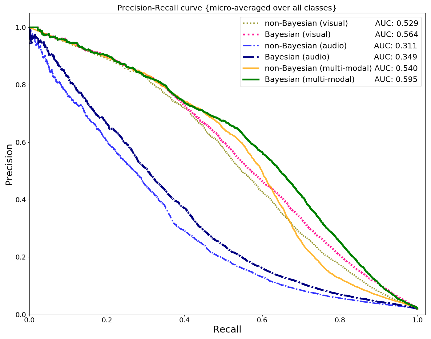
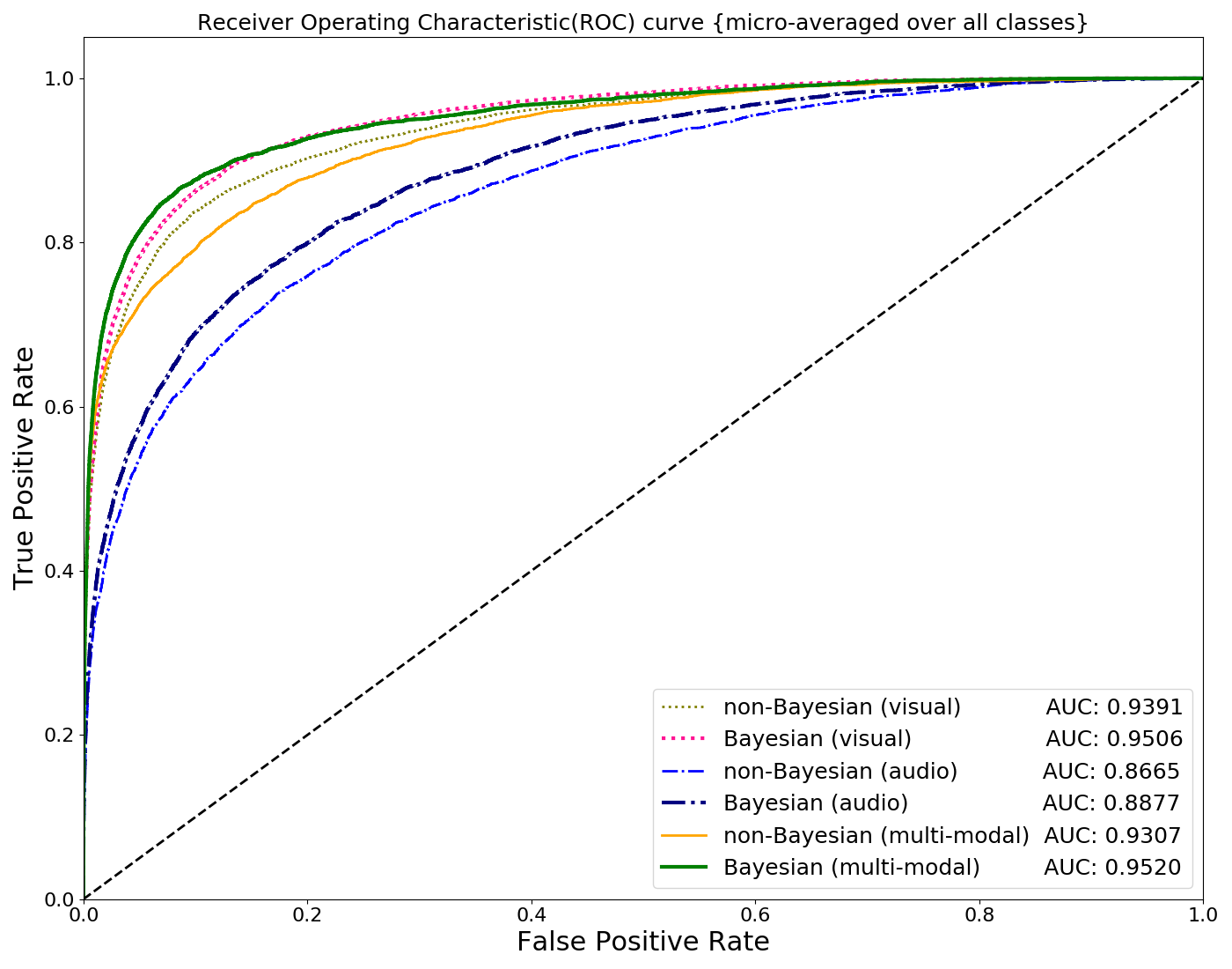
Figure 8: Precision-Recall (top) and ROC (bottom) plots micro-averaged over all the MiT in-distribution classes.

Model	Top1 (%)	Top5 (%)
Vision
DNN	52.65	79.79
Bayesian DNN (MC Dropout)	52.88	80.10
Bayesian DNN (Stochastic VI)	53.3	81.20
Audio
DNN	34.13	61.68
Bayesian DNN (MC Dropout)	32.46	60.97
Bayesian DNN (Stochastic VI)	35.80	63.40
Audiovisual
DNN	56.61	79.39
Bayesian DNN (MC-Dropout)	55.04	80.34
Bayesian DNN (Stochastic VI)	58.2	83.8

Table 1: Comparison of accuracies for DNN, Bayesian DNN MC Dropout and Stochastic Variational Inference (Stochastic VI) models applied to subset of MiT dataset (in-distribution classes).

4.2 Model performance comparison

The classification accuracy for MiT in-distribution samples is presented in Table 1. Bayesian DNN stochastic VI model consistently provides higher accuracies for individual and combined audio-vision modalities. Bayesian DNN stochastic VI audiovisual model provides an improvement of 9.2% top1 and 3.2% top5 accuracies over the Bayesian DNN visual model. Bayesian DNN stochastic VI model (audiovisual) provides an improvement of 2.8% top1 and 5.6% top5 accuracies over the baseline DNN model (audiovisual). The accuracies for Bayesian DNN MC dropout model are lower than the proposed Bayesian stochastic VI model.

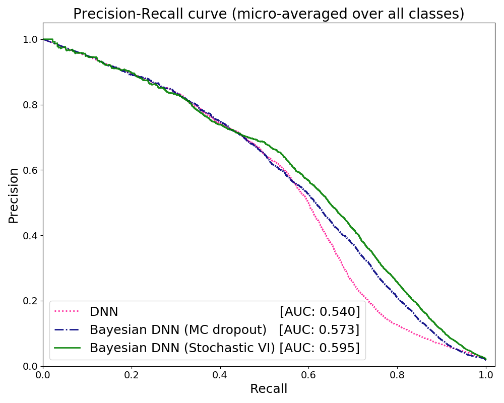
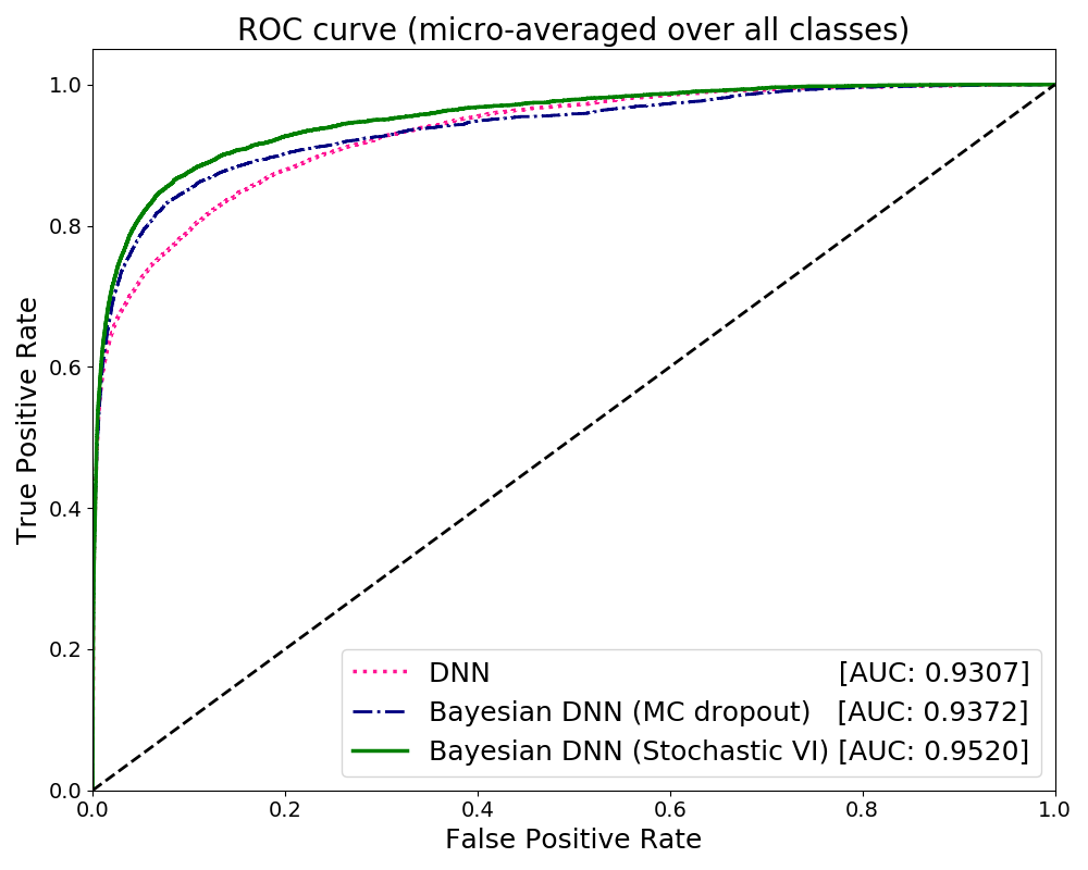
Figure 9: Precision-recall (top) and ROC (bottom) AUC plots for audiovisual models micro-averaged over all the MiT in-distribution classes.

Figure 8 shows the comparison of precision-recall and ROC plots using the confidence measures for DNN and Bayesian DNN stochastic VI models. The proposed model consistently provides higher precision-recall and ROC AUC for individual and combined audio-vision modalities. Figure 9 shows Bayesian stochastic VI audiovisual model provides precision-recall AUC improvement of 10.2% over the DNN and 3.8% over the MC Dropout audiovisual models.

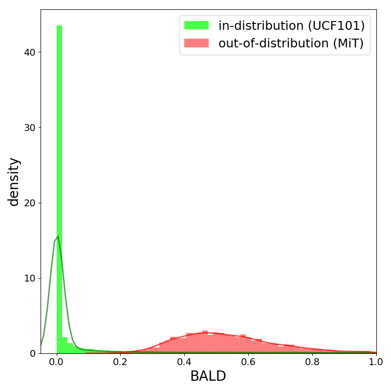
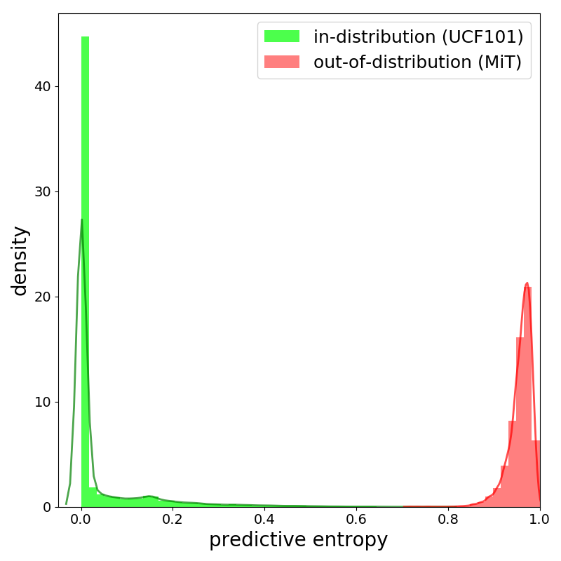
Figure 10: Density histogram of uncertainty measures (BALD and predictive entropy) obtained from Bayesian DNN stochastic VI model. In-distribution samples are from the UCF101 activity recognition dataset and out-of-distribution are from the MiT dataset. The uncertainty measures demonstrate clear separation of in- and out-of-distribution uncertainty distributions. [The density histogram has area normalized to one. Plots are overlaid with kernel density curves for better readability.]

We also compared the uncertainty estimates obtained from the proposed Bayesian DNN stochastic VI model using two separate datasets. We compared the UCF101 visual activity recognition dataset, which has 101 activity classes, as in-distribution samples and MiT dataset (vision input) as the out-of-distribution samples. The training of the UCF101 dataset for vision input is done similar to the details provided in Section 3. The DNN (Top1: 87.5% and Top5: 97.35%) and Bayesian DNN (Top1: 88.6% and Top5: 98.25%) models provide comparable accuracy values to other results obtained for UCF101 using ResNet-101 C3D model [18]. The comparison of uncertainty measures for in-distribution and out-of-distribution samples obtained from Bayesian DNN are shown in Figure 10. Both BALD and predictive entropy (details are in Section 2) uncertainty measures indicate a clear separation of uncertainty scores for in- and out-of-distribution samples.

These results confirm that the proposed Bayesian DNN stochastic VI model provides reliable confidence measure than the conventional DNN for the audiovisual activity recognition and can identify out-of-distribution samples.

5 Conclusions

Effective multimodal activity recognition requires the underlying system to intelligently decide the relative importance of each modality. Bayesian inference provides a systematic way to quantify uncertainty in the deep learning model predictions. Uncertainty estimates obtained from Bayesian DNNs can identify inherent ambiguity in individual modalities, which in turn can benefit multimodal fusion. In this work, we proposed a novel uncertainty-aware multimodal fusion method using Bayesian DNN architecture that combines deterministic and variational layers. We evaluate the proposed approach on audiovisual activity recognition using Moments-in-Time dataset. The results indicate Bayesian DNN can provide more reliable confidence measure compared to the conventional DNNs. The uncertainty estimates obtained from the proposed method have the potential to identify out-of-distribution data. The proposed method is scalable to deeper architectures and can be extended to other real-world multimodal applications.

References

- [1] Sami Abu-El-Haija, Nisarg Kothari, Joonseok Lee, Paul Natsev, George Toderici, Balakrishnan Varadarajan, and Sudheendra Vijayanarasimhan. Youtube-8m: A large-scale video classification benchmark. arXiv preprint arXiv:1609.08675, 2016.
- [2] Triantafyllos Afouras, Joon Son Chung, Andrew Senior, Oriol Vinyals, and Andrew Zisserman. Deep audio-visual speech recognition. arXiv preprint arXiv:1809.02108, 2018.
- [3] Relja Arandjelovic, Petr Gronat, Akihiko Torii, Tomas Pajdla, and Josef Sivic. Netvlad: Cnn architecture for weakly supervised place recognition. In Proceedings of the IEEE Conference on Computer Vision and Pattern Recognition, pages 5297–5307, 2016.
- [4] Yusuf Aytar, Carl Vondrick, and Antonio Torralba. See, hear, and read: Deep aligned representations. arXiv preprint arXiv:1706.00932, 2017.
- [5] Christopher M Bishop. Pattern recognition and machine learning (information science and statistics) springer-verlag new york. Inc. Secaucus, NJ, USA, 2006.
- [6] David M Blei, Alp Kucukelbir, and Jon D McAuliffe. Variational inference: A review for statisticians. Journal of the American Statistical Association, 112(518):859–877, 2017.
- [7] Charles Blundell, Julien Cornebise, Koray Kavukcuoglu, and Daan Wierstra. Weight uncertainty in neural networks. arXiv preprint arXiv:1505.05424, 2015.
- [8] Léon Bottou. Large-scale machine learning with stochastic gradient descent. In Proceedings of COMPSTAT’2010, pages 177–186. Springer, 2010.
- [9] Joao Carreira and Andrew Zisserman. Quo vadis, action recognition? a new model and the kinetics dataset. In Computer Vision and Pattern Recognition (CVPR), 2017 IEEE Conference on, pages 4724–4733. IEEE, 2017.
- [10] Jeffrey Donahue, Lisa Anne Hendricks, Sergio Guadarrama, Marcus Rohrbach, Subhashini Venugopalan, Kate Saenko, and Trevor Darrell. Long-term recurrent convolutional networks for visual recognition and description. In Proceedings of the IEEE conference on computer vision and pattern recognition, pages 2625–2634, 2015.
- [11] Matthias Dorfer, Bernhard Lehner, Hamid Eghbal-zadeh, Heindl Christop, Paischer Fabian, and Widmer Gerhard. Acoustic scene classification with fully convolutional neural networks and I-vectors. Technical report, DCASE2018 Challenge, September 2018.
- [12] Yarin Gal. Uncertainty in deep learning. University of Cambridge, 2016.
- [13] Yarin Gal and Zoubin Ghahramani. Dropout as a bayesian approximation: Representing model uncertainty in deep learning. In international conference on machine learning, pages 1050–1059, 2016.
- [14] Ruohan Gao, Rogerio Feris, and Kristen Grauman. Learning to separate object sounds by watching unlabeled video. arXiv preprint arXiv:1804.01665, 2018.
- [15] Jort F Gemmeke, Daniel PW Ellis, Dylan Freedman, Aren Jansen, Wade Lawrence, R Channing Moore, Manoj Plakal, and Marvin Ritter. Audio set: An ontology and human-labeled dataset for audio events. In Acoustics, Speech and Signal Processing (ICASSP), 2017 IEEE International Conference on, pages 776–780. IEEE, 2017.
- [16] Ian Goodfellow, Yoshua Bengio, and Aaron Courville. Deep learning. MIT press, 2016.
- [17] Alex Graves. Practical variational inference for neural networks. In Advances in neural information processing systems, pages 2348–2356, 2011.
- [18] Kensho Hara, Hirokatsu Kataoka, and Yutaka Satoh. Can spatiotemporal 3d cnns retrace the history of 2d cnns and imagenet? In Proceedings of the IEEE Conference on Computer Vision and Pattern Recognition (CVPR), pages 6546–6555, 2018.
- [19] Kaiming He, Xiangyu Zhang, Shaoqing Ren, and Jian Sun. Deep residual learning for image recognition. In Proceedings of the IEEE conference on computer vision and pattern recognition, pages 770–778, 2016.
- [20] Shawn Hershey, Sourish Chaudhuri, Daniel PW Ellis, Jort F Gemmeke, Aren Jansen, R Channing Moore, Manoj Plakal, Devin Platt, Rif A Saurous, Bryan Seybold, et al. Cnn architectures for large-scale audio classification. In Acoustics, Speech and Signal Processing (ICASSP), 2017 IEEE International Conference on, pages 131–135. IEEE, 2017.
- [21] Neil Houlsby, Ferenc Huszár, Zoubin Ghahramani, and Máté Lengyel. Bayesian active learning for classification and preference learning. arXiv preprint arXiv:1112.5745, 2011.
- [22] Michael I Jordan, Zoubin Ghahramani, Tommi S Jaakkola, and Lawrence K Saul. An introduction to variational methods for graphical models. Machine learning, 37(2):183–233, 1999.
- [23] Will Kay, Joao Carreira, Karen Simonyan, Brian Zhang, Chloe Hillier, Sudheendra Vijayanarasimhan, Fabio Viola, Tim Green, Trevor Back, Paul Natsev, et al. The kinetics human action video dataset. arXiv preprint arXiv:1705.06950, 2017.
- [24] Alex Kendall, Vijay Badrinarayanan, and Roberto Cipolla. Bayesian segnet: Model uncertainty in deep convolutional encoder-decoder architectures for scene understanding. arXiv preprint arXiv:1511.02680, 2015.
- [25] Alex Kendall and Roberto Cipolla. Modelling uncertainty in deep learning for camera relocalization. In 2016 IEEE international conference on Robotics and Automation (ICRA), pages 4762–4769. IEEE, 2016.
- [26] Alex Kendall, Yarin Gal, and Roberto Cipolla. Multi-task learning using uncertainty to weigh losses for scene geometry and semantics. arXiv preprint arXiv:1705.07115, 3, 2017.
- [27] Ranganath Krishnan, Mahesh Subedar, and Omesh Tickoo. BAR: Bayesian activity recognition using variational inference. Bayesian Deep Learning workshop, NeurIPS, 2018.
- [28] Oscar D Lara, Miguel A Labrador, et al. A survey on human activity recognition using wearable sensors. IEEE Communications Surveys and Tutorials, 15(3):1192–1209, 2013.
- [29] Annamaria Mesaros, Toni Heittola, and Tuomas Virtanen. A multi-device dataset for urban acoustic scene classification. arXiv preprint arXiv:1807.09840, 2018.
- [30] Mathew Monfort, Bolei Zhou, Sarah Adel Bargal, Alex Andonian, Tom Yan, Kandan Ramakrishnan, Lisa Brown, Quanfu Fan, Dan Gutfruend, Carl Vondrick, et al. Moments in time dataset: one million videos for event understanding. arXiv preprint arXiv:1801.03150, 2018.
- [31] Jishnu Mukhoti and Yarin Gal. Evaluating bayesian deep learning methods for semantic segmentation. arXiv preprint arXiv:1811.12709, 2018.
- [32] Radford M Neal. Bayesian learning for neural networks, volume 118. Springer Science & Business Media, 2012.
- [33] Jiquan Ngiam, Aditya Khosla, Mingyu Kim, Juhan Nam, Honglak Lee, and Andrew Y Ng. Multimodal deep learning. In Proceedings of the 28th international conference on machine learning (ICML-11), pages 689–696, 2011.
- [34] Andrew Owens and Alexei A Efros. Audio-visual scene analysis with self-supervised multisensory features. arXiv preprint arXiv:1804.03641, 2018.
- [35] Karol J Piczak. Esc: Dataset for environmental sound classification. In Proceedings of the 23rd ACM international conference on Multimedia, pages 1015–1018. ACM, 2015.
- [36] Rajesh Ranganath, Sean Gerrish, and David M Blei. Black box variational inference. arXiv preprint arXiv:1401.0118, 2013.
- [37] Michalis Raptis and Leonid Sigal. Poselet key-framing: A model for human activity recognition. In Proceedings of the IEEE Conference on Computer Vision and Pattern Recognition, pages 2650–2657, 2013.
- [38] Yuma Sakashita and Masaki Aono. Acoustic scene classification by ensemble of spectrograms based on adaptive temporal divisions. Technical report, Tech. Rep., DCASE2018 Challenge, 2018.
- [39] Amir Shahroudy, Tian-Tsong Ng, Yihong Gong, and Gang Wang. Deep multimodal feature analysis for action recognition in rgb+ d videos. IEEE Transactions on Pattern Analysis and Machine Intelligence, 40(5):1045–1058, 2018.
- [40] Gunnar A Sigurdsson, Olga Russakovsky, and Abhinav Gupta. What actions are needed for understanding human actions in videos? In Computer Vision (ICCV), 2017 IEEE International Conference on, pages 2156–2165. IEEE, 2017.
- [41] Karen Simonyan and Andrew Zisserman. Two-stream convolutional networks for action recognition in videos. In Advances in neural information processing systems, pages 568–576, 2014.
- [42] Nitish Srivastava and Ruslan Salakhutdinov. Learning representations for multimodal data with deep belief nets. In International conference on machine learning workshop, volume 79, 2012.
- [43] Christian Szegedy, Wei Liu, Yangqing Jia, Pierre Sermanet, Scott Reed, Dragomir Anguelov, Dumitru Erhan, Vincent Vanhoucke, and Andrew Rabinovich. Going deeper with convolutions. In Proceedings of the IEEE conference on computer vision and pattern recognition, pages 1–9, 2015.
- [44] Du Tran, Lubomir Bourdev, Rob Fergus, Lorenzo Torresani, and Manohar Paluri. Learning spatiotemporal features with 3d convolutional networks. In Proceedings of the IEEE international conference on computer vision, pages 4489–4497, 2015.
- [45] Du Tran, Heng Wang, Lorenzo Torresani, Jamie Ray, Yann LeCun, and Manohar Paluri. A closer look at spatiotemporal convolutions for action recognition. In Proceedings of the IEEE conference on Computer Vision and Pattern Recognition, pages 6450–6459, 2018.
- [46] Limin Wang, Yuanjun Xiong, Zhe Wang, Yu Qiao, Dahua Lin, Xiaoou Tang, and Luc Van Gool. Temporal segment networks: Towards good practices for deep action recognition. In European Conference on Computer Vision, pages 20–36. Springer, 2016.
- [47] Max Welling and Yee W Teh. Bayesian learning via stochastic gradient langevin dynamics. In Proceedings of the 28th International Conference on Machine Learning (ICML-11), pages 681–688, 2011.
- [48] Yeming Wen, Paul Vicol, Jimmy Ba, Dustin Tran, and Roger Grosse. Flipout: Efficient pseudo-independent weight perturbations on mini-batches. arXiv preprint arXiv:1803.04386, 2018.
- [49] Yuan Yuan, Xiaodan Liang, Xiaolong Wang, Dit-Yan Yeung, and Abhinav Gupta. Temporal dynamic graph lstm for action-driven video object detection. In ICCV, pages 1819–1828, 2017.
- [50] Hossein Zeinali, Lukas Burget, and Honza Cernocky. Convolutional neural networks and x-vector embedding for dcase2018 acoustic scene classification challenge. Technical report, DCASE2018 Challenge, September 2018.
- [51] Bolei Zhou, Alex Andonian, Aude Oliva, and Antonio Torralba. Temporal relational reasoning in videos. In Proceedings of the European Conference on Computer Vision (ECCV), pages 803–818, 2018.
- [52] Bolei Zhou, Alex Andonian, and Antonio Torralba. Temporal relational reasoning in videos. arXiv preprint arXiv:1711.08496, 2017.
- [53] Maryam Ziaeefard and Robert Bergevin. Semantic human activity recognition: a literature review. Pattern Recognition, 48(8):2329–2345, 2015.