Renormalization on the fuzzy sphere

Abstract:

We study renormalization on the fuzzy sphere, which is a typical example of non-commutative spaces. We numerically simulate a scalar field theory on the fuzzy sphere, which is described by a Hermitian matrix model. We define correlation functions by using the Berezin symbol and show that they are made independent of the matrix size, which plays a role of a UV cutoff, by tuning one parameter of the theory. We also find that the theories on the phase boundary are universal. They behave as a conformal field theory at short distances, while they universally differ from it at long distances due to the UV/IR mixing.

1 Introduction

It is known that field theories on non-commutative spaces are deeply involved in quantum gravity or string theory (for a review, see [1]). One of the most characteristic phenomena in field theories on non-commutative spaces is the so-called UV/IR mixing [2], which prevents perturbative renormalization.

It is important to resolve the problem of renormalization in order to construct consistent quantum field theories on non-commutative spaces. It was shown by Monte Carlo simulation in [3, 4] that the 2-point and 4-point correlation functions in the disordered phase of a scalar field theory on the fuzzy sphere are made independent of the matrix size up to a wave function renormalization by tuning a parameter in the theory, where the matrix size is regarded as a UV cutoff. This strongly suggests that the theory is non-perturbatively renormalizable in the disordered phase.

Here, we perform further study of the scalar field theory on the fuzzy sphere by Monte Carlo simulation [4]. Multi-point correlation functions are defined by using the Berezin symbol [21] in the same way as in [3]. Then, the phase boundary is identified by calculating the susceptibility which is an order parameter for the $Z_{2}$ symmetry, and the 2-point and 4-point correlation functions are calculated on the boundary. It is found that the correlation functions at different points on the boundary agree so that the theories on the boundary are universal as in ordinary field theories. Furthermore, we find that the behavior of the 2-point correlation functions is the same as that in a conformal field theory (CFT) at short distances but different from it at long distances.

2 Scalar field theory on the fuzzy sphere

We study the following matrix model:

$$S=\frac{1}{N}\mbox{Tr}\left(-\frac{1}{2}[\hat{L}_{i},\Phi]^{2}+\frac{\mu^{2}}{2}\Phi^{2}+\frac{\lambda}{4}\Phi^{4}\right)\ ,$$ (1)

where $\Phi$ is an $N\times N$ Hermitian matrix, and $N\times N$ matrices $\hat{L}_{i}$ ($i=1,2,3$) are the generators of the $SU(2)$ algebra in the $N$-dimensional irreducible representation, which satisfy the commutation relation $[\hat{L}_{i},\hat{L}_{j}]=i\epsilon_{ijk}\hat{L}_{k}$. The theory possesses $Z_{2}$ symmetry: $\Phi\rightarrow-\Phi$. The path-integral measure is defined by $d\Phi e^{-S}$, where

$$d\Phi=\prod_{i=1}^{N}d\Phi_{ii}\prod_{1\leq j<k\leq N}d\mbox{Re}\Phi_{jk}d\mbox{Im}\Phi_{jk}\ .$$ (2)

At the tree level in the $N\rightarrow\infty$ limit, which corresponds to the so-called commutative limit, the theory (1) reduces to the following continuum theory on a sphere with the radius $R$:

$$S_{\mathrm{C}}=\int\frac{R^{2}d\Omega}{4\pi}\left(-\frac{1}{2R^{2}}({\cal L}_{i}\phi(\Omega))^{2}+\frac{m^{2}}{2}\phi(\Omega)^{2}+\frac{g}{4}\phi(\Omega)^{4}\right)$$ (3)

with the invariant measure on the sphere $d\Omega$ and the orbital angular momentum operators ${\cal L}_{i}$ ($i=1,2,3$).

In the above correspondence, the Berezin symbol $\langle\Omega|\Phi|\Omega\rangle$, which is explained in the next section, is identified with the field $\phi(\Omega)$, and the parameters in (1) correspond to those in (3) as $\mu^{2}=R^{2}m^{2},\ \lambda=R^{2}g$. The authors of [22, 23] showed that the 1-loop effective action of (1) differs from that of (3) by a finite amount.

3 Correlation functions

We define correlation functions by introducing the Berezin symbol [21] constructed from the Bloch coherent state [24]. The sphere is parametrized by the standard polar coordinates $\Omega=(\theta,\varphi)$. The Bloch coherent state $|\Omega\rangle$ is localized around the point on the sphere, $(\theta,\varphi)$, with the width $R/\sqrt{N}$. For an $N\times N$ matrix $M$, the Berezin symbol is defined by $\langle\Omega|M|\Omega\rangle$.

In the following, we denote the Berezin symbol shortly as $\varphi(\Omega)=\langle\Omega|\Phi|\Omega\rangle$. Then, the $n$-point correlation function in the theory (1) is defined as

$$\left\langle\varphi(\Omega_{1})\varphi(\Omega_{2})\cdots\varphi(\Omega_{n})\right\rangle=\frac{\int d\Phi\ \varphi(\Omega_{1})\varphi(\Omega_{2})\cdots\varphi(\Omega_{n})e^{-S}}{\int d\Phi\ e^{-S}}\ .$$ (1)

This correlation function is a counterpart of $\langle\phi(\Omega_{1})\phi(\Omega_{2})\cdots\phi(\Omega_{n})\rangle$ in the theory (3).

We assume the matrix $\Phi$ in (1) to be renormalized as $\Phi=\sqrt{Z}\Phi_{\mathrm{r}}$ with the renormalized matrix $\Phi_{\mathrm{r}}$. Then, the renormalized Berezin symbol is defined by $\varphi(\Omega)=\sqrt{Z}\varphi_{\mathrm{r}}(\Omega)$, and the renormalized $n$-point correlation function is defined by

$$\left\langle\varphi(\Omega_{1})\varphi(\Omega_{2})\cdots\varphi(\Omega_{n})\right\rangle=Z^{\frac{n}{2}}\left\langle\varphi_{\mathrm{r}}(\Omega_{1})\varphi_{\mathrm{r}}(\Omega_{2})\cdots\varphi_{\mathrm{r}}(\Omega_{n})\right\rangle\ .$$ (2)

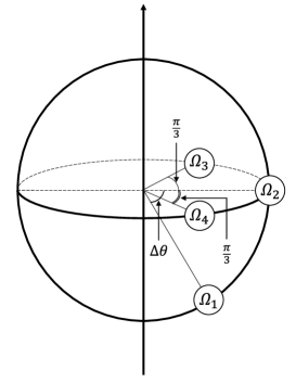
Figure 1: Four points on the sphere chosen for the correlation functions.

In the following, we calculate the following correlation functions:

$$\mbox{2-point function:}\;\left\langle\varphi(\Omega_{\rho})\varphi(\Omega_{\sigma})\right\rangle_{\mathrm{c}}\;(1\leq\rho<\sigma\leq 4)\ ,$$

$$\mbox{4-point function:}\;\left\langle\varphi(\Omega_{1})\varphi(\Omega_{2})\varphi(\Omega_{3})\varphi(\Omega_{4})\right\rangle_{\mathrm{c}}\ ,$$ (3)

where c stands for the connected part.

We pick up four points $\Omega_{\rho}=(\theta_{\rho},\varphi_{\rho})$ ($\rho=1,\ldots,4$) on the sphere as follows (see Fig. 1):

$$\Omega_{1}=\left(\frac{\pi}{2}+\Delta\theta,\ 0\right)\ ,\quad\Omega_{2}=\left(\frac{\pi}{2},\ 0\right)\ ,\quad\Omega_{3}=\left(\frac{\pi}{2},\ \frac{\pi}{3}\right)\ ,\quad\Omega_{4}=\left(\frac{\pi}{2},\ \frac{5\pi}{3}\right)\ .$$ (4)

We apply the hybrid Monte Carlo method to our simulation of the theory.

3.1 Critical behavior of correlation functions

We calculate the 2-point and 4-point correlation functions on the phase boundary at $N=24$. To determine the phase boundary, we calculate the susceptibility $\chi\equiv\left\langle\left(\mbox{Tr}\Phi/N\right)^{2}\right\rangle-\left\langle\left|\mbox{Tr}\Phi\right|/N\right\rangle^{2}$ that is an order parameter for the $Z_{2}$ symmetry which is a symmetry under $\Phi\to-\Phi$. In Fig.2, $\chi$ is plotted against $-\mu^{2}$ for $\lambda=0.5,0.6,0.7$. We find that the peak of $\chi$ for $\lambda=0.5,0.6,0.7$ exists around $\mu^{2}=-10.8,-12.8,-14.8$, respectively. The theory is in the unbroken phase in the left side of the peak, while it is in the broken phase in the right side of the peak.

We calculate 2-point and 4-point correlation functions at various $\mu^{2}$ around the above values for each $\lambda$, and find that the correlation functions for $(\mu^{2},\lambda)=(-10.801,0.5),(-12.810,0.6)$, $(-14.925,0.7)$ agree after performing wave function renormalization. In the following, we show that this is indeed in the case.

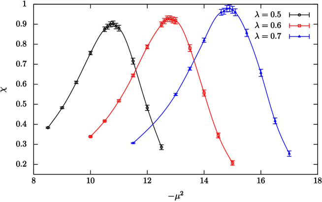
Figure 2: We plot the susceptibility $\chi$ at $N=24$ against $-\mu^{2}$. The circles, the squares, and the triangles represent the data for $\lambda=0.5,0.6,0.7$, respectively. There are the peaks of $\chi$ for $\lambda=0.5,0.6,0.7$ around $\mu^{2}=-10.8,-12.8,-14.8$, respectively.

For later convenience, we introduce a stereographic projection defined by $z=R\tan\frac{\theta}{2}e^{i\varphi}$, which maps a sphere with the radius $R$ to the complex plane. Here, $R$ is fixed at $1$ without loss of generality. We calculate $\langle\varphi(z_{m})\varphi(1)\rangle_{\mathrm{c}}$ and $\langle\varphi(z_{m})\varphi(1)\varphi(e^{i\frac{\pi}{3}})\varphi(e^{i\frac{5\pi}{3}})\rangle_{\mathrm{c}}$, where $z_{m}=\tan\left[\frac{1}{2}\left(\frac{\pi}{2}+0.1m\right)\right]$ with $m=1,\ldots,15$.

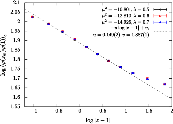
Figure 3: $\log\langle\varphi(z_{m})\varphi(1)\rangle_{\mathrm{c}}$ at $N=24$ is plotted against $\log|z-1|$. The circles, the squares, and the triangles represent the data for $\lambda=0.5,0.6,0.7$, respectively. The data for $\lambda=0.6,0.7$ are simultaneously shifted by $\alpha_{0.6\to 0.5}=-0.015(1)$ and $\alpha_{0.7\to 0.5}=-0.056(1)$, respectively, in the vertical direction so that they agree with the data for $\lambda=0.5$. The dashed line is a fit of seven data points (from the second point to the eighth point) of $\log\langle\varphi(z_{m})\varphi(1)\rangle_{\mathrm{c}}$ at $\lambda=0.5$ to $-u\log|z-1|+v$ with $u=0.149(2)$ and $v=1.887(1)$.

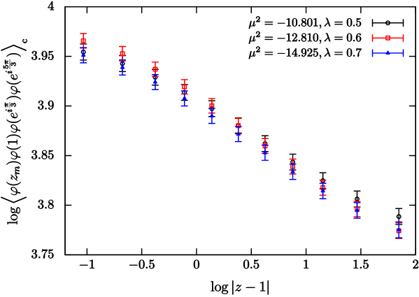
Figure 4: $\log\langle\varphi(z_{m})\varphi(1)\varphi(e^{i\frac{\pi}{3}})\varphi(e^{i\frac{5\pi}{3}})\rangle_{\mathrm{c}}$ at $N=24$ is plotted against $\log|z-1|$. The circles, the squares, and the triangles represent the data for $\lambda=0.5,0.6,0.7$, respectively. The data for $\lambda=0.6,0.7$ are simultaneously shifted by $2\alpha_{0.6\to 0.5}$ and $2\alpha_{0.7\to 0.5}$, respectively, in the vertical direction so that they agree with the data for $\lambda=0.5$.

In Fig.3, we plot $\log\langle\varphi(z_{m})\varphi(1)\rangle_{\mathrm{c}}$ against $\log|z-1|$ for $\lambda=0.5,0.6,0.7$, where the data for $\lambda=0.6,0.7$ are simultaneously shifted in the vertical direction by $\alpha_{0.6\to 0.5}=\log[Z(\lambda=0.5)/Z(\lambda=0.6)]=-0.015(1)$ and $\alpha_{0.7\to 0.5}=-0.056(1)$, respectively, so that they agree with the data for $\lambda=0.5$. In Fig.4, we also plot $\log\langle\varphi(z_{m})\varphi(1)\varphi(e^{i\frac{\pi}{3}})\varphi(e^{i\frac{5\pi}{3}})\rangle_{\mathrm{c}}$ against $\log|z-1|$ for $\lambda=0.5,0.6,0.7$, where the data for $\lambda=0.6,0.7$ are simultaneously shifted in the vertical direction by $2\alpha_{0.6\to 0.5}$ and $2\alpha_{0.7\to 0.5}$, respectively, so that they agree with the data for $\lambda=0.5$. These shifts correspond to a wave function renormalization. Namely, 2-point and 4-point correlation functions agree after performing wave function renormalization. Therefore, the above results indicates that the theories are universal on the phase boundary as in ordinary field theories. We do not see the above agreement of the correlation functions in either the UV region with $m=1,2$, or the IR region with $m=14,15$. We consider the disagreement in the latter region to be caused by increase of the ambiguity of the position on the fuzzy sphere due to the stereographic projection for large $|z|$.

Finally, we see a connection of the theory we have studied to a CFT. In Fig.3, we fit seven data points ($m=4,\ldots,10$) of $\log\langle\varphi(z_{m})\varphi(1)\rangle_{\mathrm{c}}$ for $\lambda=0.5$ to $-u\log|z-1|+v$ and obtain $u=0.149(2)$ and $v=1.887(1)$. This means that the 2-point correlation function behaves as

$$\langle\varphi(z)\varphi(1)\rangle_{\mathrm{c}}=\frac{e^{v}}{|z-1|^{u}}\quad\mathrm{for}\ \ m=4,\ldots,10\ .$$ (5)

In CFTs, the 2-point correlation function of the operator $\mathcal{O}(z)$ with the scaling dimension $\Delta$ behaves as $\left\langle\mathcal{O}(z)\mathcal{O}(z^{\prime})\right\rangle\sim 1/|z-z^{\prime}|^{2\Delta}$. Thus, the present theory on the phase boundary behaves as a CFT in the UV region. Our 2-point correlation function deviates universally from that in the CFT in the IR region with $11\leq m\leq 13$. Moreover, in a further UV region with $m=3$, it also deviates universally. We consider these deviations to be an effect of the UV/IR mixing. It is nontrivial that we observe the behavior of the CFT because field theories on non-commutative spaces are non-local ones.

4 Conclusion and discussion

We have studied renormalization in the scalar filed theory on the fuzzy sphere by Monte Carlo simulation. We examined the 2-point and 4-point correlation functions on the phase boundary where the spontaneous $Z_{2}$ symmetry breaking occurs. We found the agreement of correlation functions at different points on the boundary up to the wave function renormalization. This implies that the critical theory is universal, which is consistent with the universality in the disordered phase [3, 4], because the phase boundary is obtained by one parameter fine-tuning. Moreover, it was observed that the behavior of the 2-point correlation functions is the same as that in a CFT at short distances and universally different from that at long distances. We consider the latter to be due to the UV/IR mixing.

The CFT observed at short distances seems to be different from the critical Ising model, because the value of $u/2$ in (5) disagrees with the scaling dimension of the spin operator, $\Delta_{\mathrm{Ising}}=1/8$. This indicates that the universality classes of the scalar field theory on the fuzzy sphere are totally different from those of an ordinary field theory.

In fact, the authors of [5, 6, 7, 9, 8] reported that there exists a novel phase in the theory on the fuzzy sphere that is called the non-uniformly ordered phase [25, 26]. We hope to clarify the universality classes by studying renormalization in the whole phase diagram.

- [1] M. R. Douglas and N. A. Nekrasov, Rev. Mod. Phys. 73, 977 (2001) [hep-th/0106048].
- [2] S. Minwalla, M. Van Raamsdonk and N. Seiberg, JHEP 0002, 020 (2000) [hep-th/9912072].
- [3] K. Hatakeyama and A. Tsuchiya, PTEP 2017, no. 6, 063B01 (2017) [arXiv:1704.01698 [hep-th]].
- [4] K. Hatakeyama, A. Tsuchiya and K. Yamashiro, PTEP 2018, no. 6, 063B05 (2018) [arXiv:1805.03975 [hep-th]].
- [5] X. Martin, JHEP 0404, 077 (2004) [hep-th/0402230].
- [6] M. Panero, JHEP 0705, 082 (2007) [hep-th/0608202].
- [7] M. Panero, SIGMA 2, 081 (2006) [hep-th/0609205].
- [8] C. R. Das, S. Digal and T. R. Govindarajan, Mod. Phys. Lett. A 23, 1781 (2008) [arXiv:0706.0695 [hep-th]].
- [9] F. Garcia Flores, X. Martin and D. O’Connor, Int. J. Mod. Phys. A 24, 3917 (2009) [arXiv:0903.1986 [hep-lat]].
- [10] S. Vaidya and B. Ydri, Nucl. Phys. B 671, 401 (2003) [hep-th/0305201].
- [11] D. O’Connor and C. Saemann, JHEP 0708, 066 (2007) [arXiv:0706.2493 [hep-th]].
- [12] V. P. Nair, A. P. Polychronakos and J. Tekel, Phys. Rev. D 85, 045021 (2012) [arXiv:1109.3349 [hep-th]].
- [13] J. Tekel, Phys. Rev. D 87, no. 8, 085015 (2013) [arXiv:1301.2154 [hep-th]].
- [14] A. P. Polychronakos, Phys. Rev. D 88, 065010 (2013) [arXiv:1306.6645 [hep-th]].
- [15] J. Tekel, JHEP 1410, 144 (2014) [arXiv:1407.4061 [hep-th]].
- [16] C. Saemann, JHEP 1504, 044 (2015) [arXiv:1412.6255 [hep-th]].
- [17] S. Kawamoto and T. Kuroki, JHEP 1506, 062 (2015) [arXiv:1503.08411 [hep-th]].
- [18] J. Tekel, JHEP 1512, 176 (2015) [arXiv:1510.07496 [hep-th]].
- [19] W. Bietenholz, F. Hofheinz and J. Nishimura, JHEP 0406, 042 (2004) [hep-th/0404020].
- [20] H. Mejía-Díaz, W. Bietenholz and M. Panero, JHEP 1410, 56 (2014) [arXiv:1403.3318 [hep-lat]].
- [21] F. A. Berezin, Commun. Math. Phys. 40, 153 (1975).
- [22] C. S. Chu, J. Madore and H. Steinacker, JHEP 0108, 038 (2001) [hep-th/0106205].
- [23] H. C. Steinacker, Nucl. Phys. B 910, 346 (2016) [arXiv:1606.00646 [hep-th]].
- [24] J. P. Gazeau, Coherent States in Quantum Physics (Wiley, Weinheim, 2009).
- [25] S. S. Gubser and S. L. Sondhi, Nucl. Phys. B 605, 395 (2001) [hep-th/0006119].
- [26] J. Ambjorn and S. Catterall, Phys. Lett. B 549, 253 (2002) [hep-lat/0209106].