QCD GLUON VERTICES FROM THE STRING-INSPIRED FORMALISM

Abstract

The Bern-Kosower formalism, developed around 1990 as a novel way of obtaining QCD amplitudes as the limit of infinite string tension of the corresponding string amplitudes, was originally designed as an on-shell formalism. Building on early work by Strassler, the authors have recently shown that this “string-inspired formalism” is extremely efficient also as a tool for the study of off-shell amplitudes in QCD, and in particular for achieving compact form factor decompositions of the N-gluon vertices. Among other things, this formalism allows one to achieve a manifestly gauge invariant decomposition of these vertices by way of integration-by-parts, rather than the usual tedious analysis of the nonabelian off-shell Ward identities, and to combine the spin zero, half and one cases. Here, we will provide a summary of the method, as well as its application to the three- and four-gluon vertices.

PACS numbers: 11.15.-q , 12.38.-t, 12.38.Bx.

1 Introduction

Recent years have seen an explosive development in the area of the calculation of on-shell matrix elements in quantum field theory. particularly for gauge theory and gravity. A whole host of new concepts and techniques have emerged, such as unitarity-based methods [1, 2], twistors [3], BCFW recursion [4, 5], and Grassmannians [6, 7]; see [8] and [9] for recent reviews.

This sharply contrasts with the off-shell case, whose study has seen no comparable progress. Off-shell amplitudes in quantum field theory carry information that is often difficult, or even impossible, to retrieve from the on-shell S-matrix. To mention just a few examples, off-shell information is useful for the full exploitation of the renormalization group, the infrared properties of QCD [10], and the matching of perturbative information with lattice data (see, e.g., [11]). Having explicit results, or at least well-organized integral representations, for off-shell amplitudes can also be highly useful for the construction of higher-loop amplitudes, either directly or through the solution of the Schwinger-Dyson equations.

Beyond the simplest cases, off-shell amplitudes generally depend on a large numbers of Lorentz invariants, so that usually there is little hope for an explicit closed-form evaluation. The challenge is then rather to obtain integral representations that are amenable to numerical evaluation, and well-adapted to the symmetries of the amplitude. In gauge theory or gravity, an important part of this task is to find a tensor decomposition in the polarization indices well-organized with respect to the off-shell Ward identities.

At the three-point level, a first systematic investigation of this problem was undertaken by Ball and Chiu in 1980. In [12] they studied the vertex functions of scalar and spinor QED, and derived tensor decompositions consistent with the Ward identities and free of kinematic singularities. The coefficient functions were calculated at the one-loop order. In [13] the same authors then did a completely analogous study of the three-gluon vertex, and, in particular, found for it a decomposition in terms of six tensor structures, or “form factors”, A,B,C,F, H, and S, where the last one actually turned out to be absent at one-loop. Of the others only the tensors F and H are transversal.

Although the actual calculations of [12, 13] were at the one-loop level, the obtained tensor decompositions (“Ball-Chiu-decompositions”) are of a universal character; only the coefficient functions of the various tensor structures will change at higher loop orders in perturbation theory. It is therefore of considerable importance to obtain such decompositions also for the higher-point gluon vertices, i.e., the $N$ - gluon QCD amplitudes (recall that, in the off-shell case, it is the one-particle irreducible (‘1PI’) amplitudes that constitute the natural carriers of information in quantum field theory).

It turns out, however, that the traditional way of deriving such tensor decompositions in gauge theory, based on the explicit analysis of the off-shell Ward identities, becomes extremely cumbersome beyond the three-gluon case. Clearly some method is called for that would allow one to perform such a construction without having to solve the Ward identities.

In a series of papers the present authors have developed such a method, based on earlier work by Bern and Kosower, and Strassler. Its essential feature is, that gauge-invariant structures are generated through certain integration-by-parts (‘IBP’) at the parameter integral level. Around 1990, Bern and Kosower [14, 15, 16] developed their well-known “Bern-Kosower formalism”, which allowed them to derive a new set of “Bern-Kosower rules” for the construction of one-loop QCD amplitudes by an analysis of the field theory limit of the corresponding amplitudes in string theory. An essential technical ingredient of those rules is an IBP algorithm that has a homogenizing effect on the integrands appearing in this limit, and allows one to use the underlying worldsheet supersymmetry to relate the contributions of different spins in the loop.

This formalism was restricted to the on-shell case, but shortly afterwards Strassler [17] constructed a similar formalism inside field theory, using the worldline path integral representation of the effective action as a starting point. Since the effective action is just the generating function of the 1PI Green’s functions, this formalism is naturally geared towards the study of those. In a remarkable but unpublished paper [18] Strassler then showed, that the IBP algorithm used in the Bern-Kosower formalism also leads to the automatic appearance of gauge-invariant structures in the effective action at the integrand level. Specifically, gauge fields $A^{\mu}$ are found to assemble into nonabelian field strength tensors (see A for our conventions)

$$F_{{\mu\nu}}\equiv F_{{\mu\nu}}^{a}T^{a}=(\partial_{\mu}A_{\nu}^{a}-\partial_{\nu}A_{\mu}^{a})T^{a}+ig[A_{\mu}^{b}T^{b},A_{\nu}^{c}T^{c}]\,,$$ (1)

where the terms linear in $A^{\mu}$ appear in the bulk, and the commutator term arises as a boundary term in the IBP. Strassler considered only the low-energy limit of the effective action, and the corresponding low-energy limit of the one-loop gluon amplitudes.

In [19] we applied the same methods, with some improvements on the IBP procedure [21, 20], to the three-gluon amplitudes at full momentum, and showed that indeed it provides an extremely simple and elegant way of rederiving the Ball-Chiu decomposition, as well as its coefficient functions at one loop, without the use of the Ward identity. And it allows one to relate the spin zero, half and one contributions to the amplitude by the same “replacement rules” that are part of the Bern-Kosower rules. Moreover, at the three-point level there are already ambiguities in the IBP which can be used to optimize the integrand either with respect to gauge invariance, or with respect to transversality. The first representation, called “Q-representation” [20], arising from the most straightforward way of carrying out the IBP procedure, allows for a direct match of the vertex with the effective action; the second one, called “S-representation”, is the one that matches with the Ball-Chiu decomposition, and is characterized by manifest transversality of the integrand in the bulk, the whole non-transversality of the one-loop vertex having been absorbed into the boundary terms appearing in the IBP. In terms of the structures A, B, C, F, H this means that the transversal ones, F and H, arise from the bulk integrand, and the non-transversal ones A, B, and C as boundary terms.

In [22, 23] we applied this method to the four-gluon vertex, and found everything to work quite the same way as in the three-point case: The IBP procedure leads, at the integrand level, to a decomposition of the 1PI amplitude in terms of 19 tensor structures, well-organized with respect to gauge invariance, and unifying the spin 0, half, and one cases. Of these 19 form factors, only 14 are true four-point form factors (in the sense that their coefficient functions are given by typical four-point tensor parameter integrals, depending on the full set of kinematic invariants), while the remaining five arise as boundary terms. In the four-point case, one has to already distinguish betweens single and double boundary terms, given by three-point and two-point parameter integrals, respectively, and of those five form factors two are of the first, three of the second kind. The Q-representation can be matched to the effective action, while the S-representation has the property that all bulk terms are manifestly transversal at the integrand level, so that it can be considered as the four-point generalization of the Ball-Chiu decomposition. For the S-representation the five “boundary form factors” are just the structures A, B, C, F, H again, now reappearing with “pinched” momenta, F and H arising as single and A, B, C as double boundary terms.

The purpose of the present article is to review and summarize these recent results. Its structure is the following: In section 2 we collect some generalities on the $N$-gluon vertices, and review previous work on the three-gluon and four-gluon cases (little or nothing seems to have been done yet beyond the four-gluon case). In section 3 we review the Ball-Chiu decomposition of the three-gluon vertex. In section 4 we summarize the work of Bern and Kosower, and in section 5 describe the approach based on worldline path integrals, on which our method is based. In section 6 we discuss the IBP procedure, which is the technical centerpiece of this formalism. In section 7 we present our rederivation of the three-point Ball-Chiu decomposition, and in section 8 our novel representation of the four-gluon vertex. The resulting tensor decomposition of the four-gluon vertex is given in section 9, and a list of the corresponding one-loop parameter integrals in section 10. Our conclusions are given in section 11.

2 The N-gluon vertices

Recall, that in non-abelian gauge theory one has the Lagrangian

$${\cal L}=-{1\over 4}F^{a}_{{\mu\nu}}F^{a{\mu\nu}}\,,$$ (2)

with the non-abelian field strength tensor (1). The terms quadratic in $A_{\mu}$ provide the kinetic term, while the terms involving the commutator produce a three-gluon vertex

$$V_{\mu_{1}\mu_{2}\mu_{3}}^{a_{1}a_{2}a_{3}}=-igf^{a_{1}a_{2}a_{3}}\bigl{[}g_{\mu_{1}\mu_{2}}(k_{1}-k_{2})_{\mu_{3}}+{\rm cycl.}\bigr{]}\,,$$ (3)

and a four-gluon vertex

$$V_{\mu_{1}\mu_{2}\mu_{3}\mu_{4}}^{a_{1}a_{2}a_{3}a_{4}} = -g^{2}\bigl{[}f^{a_{1}a_{2}e}f^{a_{3}a_{4}e}(g_{\mu_{1}\mu_{3}}g_{\mu_{2}\mu_{4}}-g_{\mu_{1}\mu_{4}}g_{\mu_{2}\mu_{3}})$$

$$\quad+f^{a_{1}a_{3}e}f^{a_{4}a_{2}e}(g_{\mu_{1}\mu_{4}}g_{\mu_{3}\mu_{2}}-g_{\mu_{1}\mu_{2}}g_{\mu_{3}\mu_{4}})$$

$$\quad+f^{a_{1}a_{4}e}f^{a_{2}a_{3}e}(g_{\mu_{1}\mu_{2}}g_{\mu_{4}\mu_{3}}-g_{\mu_{1}\mu_{3}}g_{\mu_{4}\mu_{2}})\bigr{]}\,.$$

These vertices get corrected at the one-loop level by more complicated tensor structures, but the multiplicative renormalizability predicts that the UV- divergent parts of these corrections must take the same form as these tree-level vertices. Since the tree-level vertices are tied up with the kinetic term by gauge invariance, it is clear that also the role of those UV divergences in the three-gluon and four-gluon functions must just be to covariantize the ones contained in the two-point function, the gluon propagator. We can thus anticipate that they must arise from integrals of the vacuum polarization type.

We will denote the contribution to the one-loop $N$-gluon vertex due to a particle with spin $s$ in the loop, and with the standard ordering of the gluons $(12\ldots N)$, by $\Gamma^{a_{1}a_{2}\cdots a_{N}}_{s\,\mu_{1}\ldots\mu_{N}}[\varepsilon_{1},k_{1};\ldots,\varepsilon_{N};k_{N}]$. For $s=1$ this is understood to denote the sum of the gluon and ghost loop contributions. Although we will only consider the fully off-shell case, we will nonetheless introduce polarization vectors $\varepsilon_{1},\ldots,\varepsilon_{N}$ to write

$$\Gamma_{s}^{a_{1}a_{2}\cdots a_{N}}[\varepsilon_{1},k_{1};\ldots,\varepsilon_{N};k_{N}]\equiv\varepsilon_{1}^{\mu_{1}}\cdots\varepsilon_{N}^{\mu_{N}}\Gamma^{a_{1}a_{2}\cdots a_{N}}_{s\mu_{1}\ldots\mu_{N}}[k_{1},\ldots,k_{N}]\,.$$ (5)

These polarization vectors are arbitrary, and just serve as a book-keeping device that will allow us to write some tensors in a more compact way in terms of the field strength tensors for the individual gluons.

Since our method maintains the full permutation (bose) symmetry between the gluons, it will be sufficient to consider the contribution with the standard ordering. The full amplitude is given by summing over all inequivalent (non-cyclic) permutations:

$$\Gamma_{s}[\varepsilon_{1},k_{1};\ldots,\varepsilon_{N};k_{N}]=\sum_{\pi\in S_{N}/Z_{N}}\Gamma_{s}^{a_{\pi(1)}a_{\pi(2)}\cdots a_{\pi(N)}}[\varepsilon_{\pi(1)},k_{\pi(1)};\ldots,\varepsilon_{\pi(N)};k_{\pi(N)}]\,.$$

(6)

The gluon loop contribution will depend on the gauge fixing. Our method uses a path integral representation of the gluonic effective action [17, 24] that is based on the background field method with quantum Feynman gauge. This gauge choice is known [25] to unify the gluon-loop contributions to the $N$ - gluon vertices with the ones from scalars and fermions in the loop, in the sense that they then obey the same Ward identities, namely [26, 27, 23]

$$k_{1}^{\mu_{1}}\Gamma_{s\,\mu_{1}\ldots\mu_{N}}^{a_{1}a_{2}\cdots a_{N}}[k_{1},\ldots,k_{N}] = -igf_{a_{1}a_{2}c}\Gamma^{ca_{3}a_{4}\cdots a_{N}}_{s\,\mu_{2}\ldots\mu_{N}}[k_{1}+k_{2},k_{3},\cdots,k_{N}]$$

$$-igf_{a_{1}a_{3}c}\Gamma^{a_{2}ca_{4}\cdots a_{N}}_{s\,\mu_{2}\ldots\mu_{N}}[k_{1},k_{2}+k_{3},\cdots,k_{N}]+\ldots\,.$$

These Ward identities are inhomogeneous, mapping the $N$ - gluon vertex to the $N-1$ -gluon one. For a generic gauge fixing, the right-hand-side would be different for the gluon loop case, and also involve the ghosts.

After these generalities, let us now review what has already been done on the gluon vertices for the three- and four-point cases.

The one-loop contribution to the three-gluon vertex due to a gluon in general covariant gauge was studied in 1979 by Celmaster and Gonsalves [28], although only at the symmetric point. Kim and Baker [29] calculated the ghost-ghost-gluon vertex and the gluon and ghost self-energies, and used the Ward identity to get from this an expression for the longitudinal part of the three-gluon vertex. Shortly afterwards Ball and Chiu presented their above-mentioned work on the decomposition of the three-gluon vertex at general momentum [13], where they also calculated the one-loop contribution due to a gluon in Feynman gauge. Cornwall and Papavassiliou [26] in 1989 constructed a “gauge invariant three-gluon vertex”, fulfilling the ghost-free Ward identity (LABEL:ward), through the pinch technique (see [30] for a review of this technique). Freedman et al. in 1992 studied the conformal properties of this vertex [31]. Davydychev, Osland and Tarasov [32] in 1996 calculated the gluon loop contribution to the one-loop three-gluon vertex in arbitrary covariant gauge, and also the massless fermion loop contribution. The fermion loop calculation was later generalized to the massive case by Davydychev, Osland and Saks [33]. In the already mentioned work by Binger and Brodsky [25] they studied the one-loop three-gluon vertex in various dimensions, using the background field method [34, 35]. Here besides the gluon and fermion loop cases they also included the scalar loop, as is needed for SUSY extensions of QCD. They derived various sum rules relevant to the SUSY case.

The study of the loop corrections to the four-gluon vertex also started around 1980 with the work of Pascual and Tarrach [36] who studied the four-gluon vertex coupling constant renormalization based on Weinberg’s renormalization scheme [37]. In 1986, Brandt and Frenkel [38] studied the infrared behavior of the three- and four-gluon vertices in Yang-Mills theory. In their analysis the four-gluon vertex was considered with all external gluons on-shell and transverse in the Feynman gauge for simplicity. They found that the 1PI contribution to the four-gluon vertex exhibits single- and double-pole singularities. Papavassiliou in 1993 [27] generalized the pinch-technique approach of [26] to the four-gluon case, and showed that this vertex again fulfilled the ghost-free Ward identity (LABEL:ward). In 2008, Kellermann and Fischer [39] studied the running coupling constant of the four-gluon vertex in Landau gauge for pure Yang Mills theory. They investigated the non-perturbative structure of the vertex using the Dyson-Schwinger (‘DS’) equations for several momentum configurations. A good agreement between their analytical results for the leading infrared and ultraviolet terms of the DS equation and their numerical solution was obtained.

So far no information on the full off-shell four-gluon vertex structure has been presented in previous studies. In 2014, Gracey [40] studied this structure at the symmetric point. He constructed the tensor structure of the vertex in terms of 138 Lorentz tensors which is the number of rank 4 Lorentz tensors built from the three independent external momenta and the metric. Based on the determination of the full structure of this vertex a new momentum subtraction scheme was defined. Binosi et. al [41] studied the nonperturbative structure of the 1PI part of the four-gluon vertex in the Landau gauge. In particular, they considered a subset of diagrams corresponding to the one-loop dressed diagrams with vertices to be kept at tree-level and fully dressed propagators. Their analysis was based on a very simple momentum configuration $(p,p,p,-3p)$. The infrared behavior of the gluon propagator was studied and a nonperturbative connection between the masslessness of the ghost and the shape of the gluon propagator found for certain kinematic limits. Based on this connection they also predict the same behavior for any purely gluonic $N$-point function. Within the mentioned class of diagrams and with their momentum configuration they only found two orthogonal Lorentz and color tensor structures, see [41] for more details.

Recently, Eichmann et. al [42] also considered the tensor structures of four point functions with external gauge bosons using the permutation group $S_{4}$. For the off-shell four point functions they predict 136 tensor structures. A DS study of the four-gluon vertex of Landau gauge Yang Mills theory has been carried out recently [43] based on these 136 tensorial structures. Their method of solving the DS equations used a truncation that included only leading diagrams in the ultraviolet, and lower Green functions from previous DS calculations that are in good agreements with lattice data. The running coupling constant was also studied.

At two loops, so far both the three-gluon vertex [44, 45, 46] and the four-gluon vertex [40] have been studied only for very special momentum configurations.

3 The three-gluon vertex and its Ball-Chiu decomposition

The three-gluon vertex in QCD at tree level (3) is corrected at the one-loop level by the 1PI three-gluon vertex with a spinor or gluon loop. E.g. for the spinor loop case we have the diagram shown in Fig. 1 (and a second one with the other orientation of the fermion).

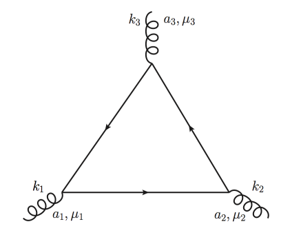
Figure 1: Three-gluon vertex.

The Ball-Chiu decomposition of the vertex is [13]

$$\Gamma_{\mu_{1}\mu_{2}\mu_{3}}(k_{1},k_{2},k_{3}) = A(k_{1}^{2},k_{2}^{2};k_{3}^{2})g_{\mu_{1}\mu_{2}}(k_{1}-k_{2})_{\mu_{3}}+B(k_{1}^{2},k_{2}^{2};k_{3}^{2})g_{\mu_{1}\mu_{2}}(k_{1}+k_{2})_{\mu_{3}}$$

$$+C(k_{1}^{2},k_{2}^{2};k_{3}^{2})[k_{1\mu_{2}}k_{2\mu_{1}}-k_{1}\cdot k_{2}g_{\mu_{1}\mu_{2}}](k_{1}-k_{2})_{\mu_{3}}$$

$$+\frac{1}{3}S(k_{1}^{2},k_{2}^{2},k_{3}^{2})(k_{1\mu_{3}}k_{2\mu_{1}}k_{3\mu_{2}}+k_{1\mu_{2}}k_{2\mu_{3}}k_{3\mu_{1}})$$

$$+F(k_{1}^{2},k_{2}^{2};k_{3}^{2})[k_{1\mu_{2}}k_{2\mu_{1}}-k_{1}\cdot k_{2}g_{\mu_{1}\mu_{2}}][k_{2\mu_{3}}k_{1}\cdot k_{3}-k_{1\mu_{3}}k_{2}\cdot k_{3}]$$

$$+H(k_{1}^{2},k_{2}^{2},k_{3}^{2})\Bigl{(}-g_{\mu_{1}\mu_{2}}[k_{1\mu_{3}}k_{2}\cdot k_{3}-k_{2\mu_{3}}k_{1}\cdot k_{3}]+\frac{1}{3}(k_{1\mu_{3}}k_{2\mu_{1}}k_{3\mu_{2}}-k_{1\mu_{2}}k_{2\mu_{3}}k_{3\mu_{1}})\Bigr{)}$$

$$+\,[\mbox{\rm cyclic permutations of }(k_{1},\mu_{1}),(k_{2},\mu_{2}),(k_{3},\mu_{3})]\,.$$

This form factor decomposition is universal, that is, valid for the scalar, spinor and gluon loop, and also for higher loop corrections. Only the coefficient functions $A,B,C,F,H,S$ change. At tree level, $A=1$, the other functions vanish. Explicit calculation shows that $S$ still vanishes at one-loop. The tensor structures multiplying $F,H$ are manifestly transversal.

4 The Bern-Kosower formalism

In 1991 Bern and Kosower in their seminal work derived, by an analysis of the infinite string limit of certain string amplitudes, the following Bern-Kosower master formula [14, 15, 16]:

$$\Gamma_{0}^{a_{1}\dots a_{N}}[k_{1},\varepsilon_{1};\dots;k_{N},\varepsilon_{N}] = (-ig)^{N}\mbox{tr}(T^{a_{1}}\dots T^{a_{N}})\int_{0}^{\infty}dT(4\pi T)^{-D/2}e^{-m^{2}T}$$

$$\times\int_{0}^{T}d\tau_{1}\int_{0}^{\tau_{1}}d\tau_{2}\dots\int_{0}^{\tau_{N-2}}d\tau_{N-1}$$

$$\times\exp\Bigg{\{}\sum_{i,j=1}^{N}\left[\frac{1}{2}G_{Bij}k_{i}\cdot k_{j}-i\dot{G}_{Bij}\varepsilon_{i}\cdot k_{j}+\frac{1}{2}\ddot{G}_{Bij}\varepsilon_{i}\cdot\varepsilon_{j}\right]\Bigg{\}}\Biggl{|}_{\rm lin(\varepsilon_{1}\ldots\varepsilon_{N})}\,.$$

As it stands, this is a parameter integral representation for the (color-ordered) 1PI $N$ - gluon amplitude induced by a scalar loop, with momenta $k_{i}$ and polarizations $\varepsilon_{i}$, in $D$ dimensions. Here $m$ and $T$ are the loop mass and proper-time, $\tau_{i}$ fixes the location of the $i$th gluon, and $G_{Bij}\equiv G_{B}(\tau_{i},\tau_{j})$ denotes the “bosonic” worldline Green’s function, defined by

$$G_{Bij} = |\tau_{i}-\tau_{j}|-\frac{(\tau_{i}-\tau_{j})^{2}}{T}\,,$$ (10)

and dots generally denote a derivative acting on the first variable. Explicitly,

$$\dot{G}_{B}(\tau_{1},\tau_{2}) = {\rm sign}(\tau_{1}-\tau_{2})-2{{(\tau_{1}-\tau_{2})}\over T}\,,$$

$$\ddot{G}_{B}(\tau_{1},\tau_{2}) = 2{\delta}(\tau_{1}-\tau_{2})-{2\over T}\,.$$

Note that this master formula has the full permutation symmetry between the $N$ - gluons. Note also that, although it is off-shell, it does not contain the Lorentz invariants $k_{i}^{2}$ and $\varepsilon_{i}\cdot k_{i}$.

In the Bern-Kosower formalism, this master formula serves as a generating functional for the full on-shell $N$ - gluon amplitudes for the scalar, spinor and gluon loop, through the use of the Bern-Kosower rules:

• For fixed $N$, expand the generating exponential and take only the terms linear in all polarization vectors.

• Use suitable integrations-by-parts (IBPs) to remove all second derivatives $\ddot{G}_{Bij}$.

• Apply two types of pattern-matching rules:

  • The “tree replacement rules” generate (from a field theory point of view) the contributions of the missing reducible diagrams.

  • The “loop replacement rules” generate the integrands for the spinor and gluon loop from the one for the scalar loop.

5 The worldline path integral formalism

Shortly after the work of Bern and Kosower, Strassler [17] rederived the master formula and the loop replacement rules using worldline path integral representations of the gluonic effective actions. E.g. for the scalar loop,

$$\Gamma[A]={\rm tr}{\displaystyle\int_{0}^{\infty}}{dT\over T}\,e^{-m^{2}T}\int{\cal D}x(\tau)\,{\cal P}e^{-\int_{0}^{T}d\tau\Bigl{(}{1\over 4}\dot{x}^{2}+ig\dot{x}\cdot A(x(\tau))\Bigr{)}}\,,\\$$

where $A_{\mu}=A_{\mu}^{a}T^{a}$ and $\cal P$ denotes path ordering. This also showed that the master formula and the loop replacement rules hold off-shell, which was not obvious from its original derivation. Moreover, in [18] Strassler noted that the IBP generates automatically abelian field strength tensors

$$f_{i}^{\mu\nu}\equiv k_{i}^{\mu}\varepsilon_{i}^{\nu}-\varepsilon_{i}^{\mu}k_{i}^{\nu}\,,$$ (12)

in the bulk, and color commutators $[T^{a_{i}},T^{a_{j}}]$ as boundary terms. Those fit together to produce full nonabelian field strength tensors (1) in the low-energy effective action. Thus we see the emergence of gauge invariant tensor structures at the integrand level.

However, the removal of all $\ddot{G}_{Bij}$ by IBP can be done in many ways, and it is not obvious how to do it in a way that would preserve also the bose symmetry between the gluons at the integrand level. In [18] Strassler started to investigate this ambiguity at the four-point level, but an algorithm valid for any $N$ and manifestly preserving the permutation invariance was found only much later [21, 47]. This algorithm still followed the objective of achieving a form of the $N$ - gluon vertex that, in $x$ - space, would correspond to a manifestly covariant representation of the nonabelian effective action. However, it turns out not be optimized from another point of view, which is important, e.g., for the Schwinger-Dyson equations, namely it does not lead to a clean separation of the vertices into transversal and longitudinal parts. This remaining obstacle has been overcome only recently in [20], where we give two IBP algorithms that work for arbitrary $N$ and lead to explicit form-factor decompositions of the off-shell $N$ - gluon amplitudes:

• The first algorithm uses only local total derivative terms and leads to a representation that matches term-by-term with the low-energy effective action (“Q-representation ”).

• The second algorithm uses both local and nonlocal total derivative terms and leads to the transversality of all bulk terms at the integrand level (“ S-representation”).

The S-representation involves $N$ reference vectors $r_{1},\ldots,r_{N}$ fulfilling $r_{i}\cdot k_{i}\neq 0$ but arbitrary otherwise. In terms of these reference vectors, the transition from the Q-representation to the S-representation can, for the bulk (but not the boundary) terms also be simply stated as the following shift of all polarization vectors:

$$\varepsilon_{i}\longrightarrow\tilde{\varepsilon}_{i}\equiv\varepsilon_{i}-\frac{\varepsilon_{i}\cdot r_{i}}{k_{i}\cdot r_{i}}k_{i}\,.$$ (13)

This makes transversality, i.e. vanishing under $\varepsilon_{i}\to k_{i}$, manifest.

In [19] we applied both algorithms to the three-point case and showed that, in particular, the second algorithm generates precisely the Ball-Chiu decomposition. Very recently, we have carried out the same program also for the much more challenging four-gluon vertex [23]. We will now sketch these rather involved calculations as well as space permits.

6 The integration-by-parts procedure

A full discussion of the IBP procedure would be too lengthy to be presented here. Thus we will show here only an example at the three-point level, and refer the reader to [20] for an exhaustive discussion. For $N=3$, the expansion of the Bern-Kosower master formula (LABEL:bk) yields

$$\Gamma_{0}^{a_{1}a_{2}a_{3}}[k_{1},\varepsilon_{1};k_{2},\varepsilon_{2};k_{3},\varepsilon_{3}] = (-ig)^{3}\mbox{tr}(T^{a_{1}}T^{a_{2}}T^{a_{3}})\int_{0}^{\infty}dT(4\pi T)^{-D/2}e^{-m^{2}T}$$

$$\times\int_{0}^{T}d\tau_{1}\int_{0}^{\tau_{1}}d\tau_{2}\,(-i)^{3}P_{3}\,e^{(G_{B12}k_{1}\cdot k_{2}+G_{B13}k_{1}\cdot k_{3}+G_{23}k_{2}\cdot k_{3})}\,,$$

where

$$P_{3} = \dot{G}_{B1i}\varepsilon_{1}\cdot k_{i}\dot{G}_{B2j}\varepsilon_{2}\cdot k_{j}\dot{G}_{B3k}\varepsilon_{3}\cdot k_{k}-\ddot{G}_{B12}\varepsilon_{1}\cdot\varepsilon_{2}\dot{G}_{B3k}\varepsilon_{3}\cdot k_{k}$$

$$-\ddot{G}_{B13}\varepsilon_{1}\cdot\varepsilon_{3}\dot{G}_{B2j}\varepsilon_{2}\cdot k_{j}-\ddot{G}_{B23}\varepsilon_{2}\cdot\varepsilon_{3}\dot{G}_{B1i}\varepsilon_{1}\cdot k_{i}\,,$$

and we have introduced the convention that repeated indices $i,j,k,\ldots$ are to be summed from 1 to $N=3$. To remove, e.g., the term involving $\ddot{G}_{B12}\dot{G}_{B31}$ in the second term of $k_{3}$, we add the total derivative

$$-\frac{\partial}{\partial\tau_{2}}\Bigl{(}\dot{G}_{B12}\varepsilon_{1}\cdot\varepsilon_{2}\dot{G}_{B31}\varepsilon_{3}\cdot k_{1}e^{(G_{B12}k_{1}\cdot k_{2}+G_{B13}k_{1}\cdot k_{3}+G_{23}k_{2}\cdot k_{3})}\Bigr{)}\,.$$ (16)

In the abelian case this total derivative term would be integrated over the full circle, and the result would be zero, since the worldline Green’s function $G_{B}(\tau_{1},\tau_{2})$ has the appropriate periodicity properties to make the two boundary terms cancel. Here instead we find a nonzero result:

$$-\dot{G}_{B12}\varepsilon_{1}\cdot\varepsilon_{2}\dot{G}_{B31}\varepsilon_{3}\cdot k_{1}e^{(\cdot)}\Big{|}_{\tau_{2}=\tau_{3}}^{\tau_{2}=\tau_{1}}=0+\dot{G}_{B13}\varepsilon_{1}\cdot\varepsilon_{2}\dot{G}_{B31}\varepsilon_{3}\cdot k_{1}e^{G_{B13}k_{1}\cdot(k_{2}+k_{3})}\,.$$

(17)

Now, in the three-point case there are already two inequivalent orderings, say, $(123)$ and $(132)$; thus the full amplitude will also have a part $\Gamma^{a_{1}a_{3}a_{2}}$ with color trace ${\rm tr}\,(T^{a_{1}}T^{a_{3}}T^{a_{2}})$, and the same total derivative term will contribute to it a boundary term

$$-\dot{G}_{B12}\varepsilon_{1}\cdot\varepsilon_{2}\dot{G}_{B31}\varepsilon_{3}\cdot k_{1}e^{(\cdot)}\Big{|}_{\tau_{2}=\tau_{1}}^{\tau_{2}=\tau_{3}}=-\dot{G}_{B13}\varepsilon_{1}\cdot\varepsilon_{2}\dot{G}_{B31}\varepsilon_{3}\cdot k_{1}e^{G_{B13}k_{1}\cdot(k_{2}+k_{3})}-0\,.$$

(18)

These two boundary terms would cancel in the abelian case, but now instead combine to produce a color commutator ${\rm tr}\,(T^{a_{1}}[T^{a_{2}},T^{a_{3}}])$. Moreover, among the other five similar total derivative terms needed to remove all the $\ddot{G}_{Bij}$s from $k_{3}$ into $Q_{3}$ there is one that differs from (16) only by the interchange $2\leftrightarrow 3$. With some relabeling of integration variables, we can combine the two boundary terms generated by that term with the two above to the structure

$${\rm tr}\,(T^{a_{1}}[T^{a_{2}},T^{a_{3}}])\varepsilon_{3}\cdot f_{1}\cdot\varepsilon_{2}\dot{G}_{B12}\dot{G}_{B21}\,e^{G_{B12}k_{1}\cdot(k_{2}+k_{3})}\,.$$ (19)

This term involves only a two-point integral, with “pinched” momenta $k_{2}+k_{3}$, and it is easy to see that its role is to provide a piece needed to extend the “abelian” Maxwell term ${\rm tr}\,(f_{{\mu\nu}}f^{{\mu\nu}})$ to the full nonabelian one ${\rm tr}\,(F_{{\mu\nu}}F^{{\mu\nu}})$.

7 The three-gluon vertex in the string-inspired formalism

We now present the final Q- and S- representations for the three-gluon vertex.

7.1 The Q-representation of the three-gluon vertex

For $N=3$, the Q-representation is (for the scalar loop) [19]

$$\Gamma = \frac{g^{3}}{(4\pi)^{\frac{D}{2}}}\mbox{tr}(T^{a_{1}}[T^{a_{2}},T^{a_{3}}])(\Gamma^{3}+\Gamma^{2}+\Gamma^{{\rm bt}})\,,$$

where

$$\Gamma^{3} = -\int_{0}^{\infty}\frac{dT}{T^{\frac{D}{2}}}e^{-m^{2}T}\int_{0}^{T}d\tau_{1}\int_{0}^{\tau_{1}}d\tau_{2}\,Q_{3}^{3}\exp\bigg{\{}\sum_{i,j=1}^{3}\frac{1}{2}G_{Bij}k_{i}\cdot k_{j}\bigg{\}}\,,$$

$$\Gamma^{2} = \Gamma^{3}(Q_{3}^{3}\to Q_{3}^{2})\,,$$

$$\Gamma^{{\rm bt}} = \int_{0}^{\infty}\frac{dT}{T^{\frac{D}{2}}}e^{-m^{2}T}\int_{0}^{T}d\tau_{1}\dot{G}_{B12}\dot{G}_{B21}\Bigl{[}\varepsilon_{3}\cdot f_{1}\cdot\varepsilon_{2}\,e^{G_{B12}k_{1}\cdot(k_{2}+k_{3})}+{\rm cycl.}\Bigr{]}\,,$$

and

$$Q_{3}^{3} = \dot{G}_{B12}\dot{G}_{B23}\dot{G}_{B31}{\rm tr}\,(f_{1}f_{2}f_{3})\,,$$

$$Q_{3}^{2} = {1\over 2}\dot{G}_{B12}\dot{G}_{B21}{\rm tr}\,(f_{1}f_{2})\dot{G}_{B3k}\varepsilon_{3}\cdot k_{k}+2\,{\rm perm}\,.$$

(22)

Here $\Gamma^{\rm bt}$ comes from the boundary terms, and the upper indices on $\Gamma^{2,3},Q^{2,3}$ refer to the “cycle content”; e.g. $Q_{3}^{3}$ contains a factor $\dot{G}_{B12}\dot{G}_{B23}\dot{G}_{B31}$ whose indices form a closed cycle involving three points, called “three-cycle”. To pass from the scalar to the spinor loop, one applies the “loop replacement rules”

$$\dot{G}_{Bij}\dot{G}_{Bji} \to \dot{G}_{Bij}\dot{G}_{Bji}-G_{Fij}G_{Fji}\,,$$

$$\dot{G}_{B12}\dot{G}_{B23}\dot{G}_{B31} \to \dot{G}_{B12}\dot{G}_{B23}\dot{G}_{B31}-G_{F12}G_{F23}G_{F31}\,,$$

where $G_{Fij}={\rm sign}(\tau_{i}-\tau_{j})$. Similarly, the integrand for the gluon loop is obtained from the scalar loop one by

$$\dot{G}_{Bij}\dot{G}_{Bji} \to \dot{G}_{Bij}\dot{G}_{Bji}-4G_{Fij}G_{Fji}\,,$$

$$\dot{G}_{B12}\dot{G}_{B23}\dot{G}_{B31} \to \dot{G}_{B12}\dot{G}_{B23}\dot{G}_{B31}-4G_{F12}G_{F23}G_{F31}\,.$$

As stated above, the gluon loop vertex obtained in this way corresponds to the background field method with quantum Feynman gauge [17, 24].

7.2 The S-representation of the three-gluon vertex

In the S-representation, the three-gluon vertex becomes

$$\tilde{\Gamma} = \frac{g^{3}}{(4\pi)^{\frac{D}{2}}}\mbox{tr}(T^{a_{1}}[T^{a_{2}},T^{a_{3}}])(\tilde{\Gamma}^{3}+\tilde{\Gamma}^{2}+\tilde{\Gamma}^{{\rm bt}})\,,$$ (25)

where

$$\tilde{\Gamma}^{3} = -\int_{0}^{\infty}\frac{dT}{T^{\frac{D}{2}}}e^{-m^{2}T}\int_{0}^{T}d\tau_{1}\int_{0}^{\tau_{1}}d\tau_{2}\,S_{3}^{3}\exp\bigg{\{}\sum_{i,j=1}^{3}\frac{1}{2}G_{Bij}k_{i}\cdot k_{j}\biggr{\}}\,,$$

$$\tilde{\Gamma}^{2} = \tilde{\Gamma}^{3}(S_{3}^{3}\to S_{3}^{2})\,,$$

$$\tilde{\Gamma}^{{\rm bt}} = \int_{0}^{\infty}\frac{dT}{T^{\frac{D}{2}}}e^{-m^{2}T}\int_{0}^{T}d\tau_{1}\dot{G}_{B12}\dot{G}_{B21}\Bigl{\{}\Bigl{[}\varepsilon_{3}\cdot f_{1}\cdot\varepsilon_{2}-{1\over 2}{\rm tr}(f_{1}f_{2})\rho_{3}+{1\over 2}{\rm tr}(f_{3}f_{1})\rho_{2}\Bigr{]}$$

$$\hskip 140.0pt\times\,e^{G_{B12}k_{1}\cdot(k_{2}+k_{3})}+\,{\rm cycl.}\Bigr{\}}\,,$$

and

$$S_{3}^{3} = \dot{G}_{B12}\dot{G}_{B23}\dot{G}_{B31}{\rm tr}\,(f_{1}f_{2}f_{3})\,,$$

$$S_{3}^{2} = {1\over 2}\dot{G}_{B12}\dot{G}_{B21}{\rm tr}\,(f_{1}f_{2})\dot{G}_{B3k}\frac{r_{3}\cdot f_{3}\cdot k_{k}}{r_{3}\cdot k_{3}}+2\,{\rm perm}\,.$$

Here we have introduced three vectors $r_{i}$, and abbreviated $\rho_{i}:=\frac{r_{i}\cdot\varepsilon_{i}}{r_{i}\cdot k_{i}}$. Note that $S^{3}_{3}$ is the same as $Q^{3}_{3}$ above, but that in $S^{2}_{3}$, contrary to $Q^{2}_{3}$, all three polarization vectors $\varepsilon_{i}$ are absorbed in abelian field strength tensors $f_{i}$. Thus all bulk terms are now manifestly transversal, and it turns out that with the cyclic choice

$$r_{1}=k_{2}-k_{3},r_{2}=k_{3}-k_{1},r_{3}=k_{1}-k_{2}\,,$$

we get a term-by-term match with the Ball-Chiu decomposition:

$$H(k_{1}^{2},k_{2}^{2},k_{3}^{2}) = C(r)\frac{g^{2}}{(4\pi)^{D/2}}\Gamma(3-\frac{D}{2})I^{D}_{3,B}(k_{1}^{2},k_{2}^{2},k_{3}^{2})\,,$$

$$A(k_{1}^{2},k_{2}^{2};k_{3}^{2}) = C(r)\frac{g^{2}}{2(4\pi)^{D/2}}\Gamma(2-\frac{D}{2})\Bigl{[}I^{D}_{{\rm bt,B}}(k_{1}^{2})+I^{D}_{{\rm bt,B}}(k_{2}^{2})\Bigr{]}\,,$$

$$B(k_{1}^{2},k_{2}^{2};k_{3}^{2}) = C(r)\frac{g^{2}}{2(4\pi)^{D/2}}\Gamma(2-\frac{D}{2})\Big{[}I^{D}_{{\rm bt,B}}(k_{1}^{2})-I^{D}_{{\rm bt,B}}(k_{2}^{2})\Big{]}\,,$$

$$F(k_{1}^{2},k_{2}^{2};k_{3}^{2}) = C(r)\frac{g^{2}}{(4\pi)^{D/2}}\Gamma(3-\frac{D}{2})\frac{I_{2,B}^{D}(k_{1}^{2},k_{2}^{2},k_{3}^{2})-I_{2,B}^{D}(k_{2}^{2},k_{1}^{2},k_{3}^{2})}{k_{1}^{2}-k_{2}^{2}}\,,$$

$$C(k_{1}^{2},k_{2}^{2};k_{3}^{2}) = C(r)\frac{g^{2}}{(4\pi)^{D/2}}\Gamma(2-\frac{D}{2})\frac{I^{D}_{{\rm bt,B}}(k_{1}^{2})-I^{D}_{{\rm bt,B}}(k_{2}^{2})}{k_{1}^{2}-k_{2}^{2}}\,,$$

$$S(k_{1}^{2},k_{2}^{2};k_{3}^{2}) = 0\,,$$

where we have used ${\rm tr}(T^{a_{1}}[T^{a_{2}},T^{a_{3}}])=iC(r)\,f^{a_{1}a_{2}a_{3}}$. The coefficient functions appearing here are

$$I_{3,B}^{D}(k_{1}^{2},k_{2}^{2},k_{3}^{2}) = \int_{0}^{1}d{\alpha}_{1}d{\alpha}_{2}d{\alpha}_{3}\delta(1-{\alpha}_{1}-{\alpha}_{2}-{\alpha}_{3})\times\frac{(1-2{\alpha}_{1})(1-2{\alpha}_{2})(1-2{\alpha}_{3})}{\Bigl{(}m^{2}+{\alpha}_{1}{\alpha}_{2}k_{1}^{2}+{\alpha}_{2}{\alpha}_{3}k_{2}^{2}+{\alpha}_{1}{\alpha}_{3}k_{3}^{2}\Bigr{)}^{3-\frac{D}{2}}}\,,$$

$$I_{2,B}^{D}(k_{1}^{2},k_{2}^{2},k_{3}^{2}) = \int_{0}^{1}d{\alpha}_{1}d{\alpha}_{2}d{\alpha}_{3}\delta(1-{\alpha}_{1}-{\alpha}_{2}-{\alpha}_{3})\times\frac{(1-2{\alpha}_{2})^{2}(1-2{\alpha}_{1})}{\Bigl{(}m^{2}+{\alpha}_{1}{\alpha}_{2}k_{1}^{2}+{\alpha}_{2}{\alpha}_{3}k_{2}^{2}+{\alpha}_{1}{\alpha}_{3}k_{3}^{2}\Bigr{)}^{3-\frac{D}{2}}}\,,$$

$$I_{bt,B}^{D}(p^{2}) = \int_{0}^{1}d{\alpha}\frac{(1-2{\alpha})^{2}}{\bigl{(}m^{2}+{\alpha}(1-{\alpha})k^{2}\bigr{)}^{2-\frac{D}{2}}}\,.$$

Here we have transformed from the integration variables $\tau_{i}$ to standard Feynman/Schwinger parameters $\alpha_{i}$ via $\tau_{1,2}=Tu_{1,2},\tau_{3}=0$ and

$$\alpha_{1} = 1-u_{1},\quad\alpha_{2}=u_{1}-u_{2},\quad\alpha_{3}=u_{2}$$ (30)

with $\sum_{i=1}^{3}\alpha_{i}=1$.

All this is written for the scalar loop case, but due to the loop replacement rules (which generalize (LABEL:spin) and (LABEL:gluon) in a straightforward way) the transition to the spinor and gluon loop cases is quite trivial, amounting only to simple algebraic changes of the numerator polynomials in (LABEL:3pointints). This is, of course, very different from the standard Feynman diagram approach, where each spin in the loop requires a separate calculation.

8 The four-gluon vertex in the string-inspired formalism

Proceeding to the four-point case, for the spinor loop case we have the diagram shown in Fig. 2 (and five more according to external gluons permutations), here the Q-representation for the scalar loop has the following bulk terms:

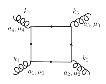
Figure 2: Four-gluon vertex.

$$\Gamma^{a_{1}a_{2}a_{3}a_{4}} = g^{4}\mbox{tr}(T^{a_{1}}\dots T^{a_{4}})\int_{0}^{\infty}dT(4\pi T)^{-D/2}e^{-m^{2}T}$$

$$\times\int_{0}^{T}d\tau_{1}\int_{0}^{\tau_{1}}d\tau_{2}\int_{0}^{\tau_{2}}d\tau_{3}Q_{4}\exp\bigg{\{}\sum_{i,j=1}^{4}\frac{1}{2}G_{Bij}k_{i}\cdot k_{j}\bigg{\}}\,,$$

where

$$Q_{4} = Q^{4}_{4}+Q^{3}_{4}+Q^{2}_{4}-Q^{22}_{4}\,,$$

$$Q^{4}_{4} = {\dot{G}}(1234)+{\dot{G}}(1243)+{\dot{G}}(1324)\,,$$

$$Q^{3}_{4} = {\dot{G}}(123)T(4)+{\dot{G}}(234)T(1)+{\dot{G}}(341)T(2)+{\dot{G}}(412)T(3)\,,$$

$$Q^{2}_{4} = {\dot{G}}(12)T(34)+{\dot{G}}(13)T(24)+{\dot{G}}(14)T(23)+{\dot{G}}(23)T(14)$$

$$+{\dot{G}}(24)T(13)+{\dot{G}}(34)T(12)\,,$$

$$Q^{22}_{4} = {\dot{G}}(12){\dot{G}}(34)+{\dot{G}}(13){\dot{G}}(24)+{\dot{G}}(14){\dot{G}}(23)\,,$$

and we have now employed a more condensed notation:

$${\dot{G}}(i_{1}i_{2}\cdots i_{n}) := {\dot{G}}_{Bi_{1}i_{2}}{\dot{G}}_{Bi_{2}i_{3}}\cdots{\dot{G}}_{Bi_{n}i_{1}}\Bigl{(}{1\over 2}\Bigr{)}^{\delta_{n,2}}{\rm tr}(f_{i_{1}}f_{i_{2}}\cdots f_{i_{n}})\,,$$

$$T(i) := \sum_{r}{\dot{G}}_{Bir}\varepsilon_{i}\cdot k_{r}\,,$$

$$T(ij) := \sum_{r,s}\Bigg{\{}{\dot{G}}_{Bir}\varepsilon_{i}\cdot k_{r}{\dot{G}}_{js}\varepsilon_{j}\cdot k_{s}+{1\over 2}{\dot{G}}_{Bij}\varepsilon_{i}\cdot\varepsilon_{j}\Big{[}{\dot{G}}_{Bir}k_{i}\cdot k_{r}-{\dot{G}}_{Bjr}k_{j}\cdot k_{r}\Big{]}\Bigg{\}}\,.$$

The IBP procedure now leads to both single boundary terms (three-point integrals) and double boundary terms (two-point integrals). The following rules emerge:

• Each single boundary term, say for the limit $3\to 4$, matches some bulk term in the Q-representation of the three-gluon vertex, with momenta $(k_{1},k_{2},k_{3}+k_{4})$, and $f_{3}=k_{3}\otimes\varepsilon_{3}-\varepsilon_{3}\otimes k_{3}$ replaced by $\varepsilon_{3}\otimes\varepsilon_{4}-\varepsilon_{4}\otimes\varepsilon_{3}$.

• Each double boundary term, say for the limit $1\to 2,3\to 4$, matches the bulk term in the Q-representation of the two-point function, with momenta $(k_{1}+k_{2},k_{3}+k_{4})$, and the double replacement

  $$f_{1} = k_{1}\otimes\varepsilon_{1}-\varepsilon_{1}\otimes k_{1}\to\varepsilon_{1}\otimes\varepsilon_{2}-\varepsilon_{2}\otimes\varepsilon_{1}\,,$$

  $$f_{2} = k_{2}\otimes\varepsilon_{2}-\varepsilon_{2}\otimes k_{2}\to\varepsilon_{3}\otimes\varepsilon_{4}-\varepsilon_{4}\otimes\varepsilon_{3}\,.$$

Moreover, this recursive structure is compatible with the replacement rules.

The S-representation looks similar, but has the bulk terms written completely in terms of the $f_{i}$, so that all non-transversality has now been absorbed into the boundary terms.

9 Tensor decomposition of the four-gluon vertex

Up to permutations compatible with the fixed color-ordering (that is, cyclic permutations and inversion) at the one-loop level 19 different structures appear in our representation. This is independent of the spin in the loop. However, as explained above of these 19 tensors five are just the two- and three-point form factors reappearing at the four-point level as boundary terms. Let us list here the remaining 14 “true” four-point tensors:

$$T^{4}_{P} = {\rm tr}\,(f_{1}f_{2}f_{3}f_{4})\,,$$

$$T^{4}_{NP} = {\rm tr}\,(f_{1}f_{3}f_{2}f_{4})\,,$$

$$T^{22}_{P} = {1\over 4}{\rm tr}\,(f_{1}f_{2}){\rm tr}\,(f_{3}f_{4})\,,$$

$$T^{22}_{NP} = {1\over 4}{\rm tr}\,(f_{1}f_{3}){\rm tr}\,(f_{2}f_{4})\,,$$

$$T^{3}_{P} = {\rm tr}\,(f_{1}f_{2}f_{3})\varepsilon_{4}\cdot k_{1}\,,$$

$$T^{3}_{NP} = {\rm tr}\,(f_{1}f_{2}f_{3})\varepsilon_{4}\cdot k_{2}\,,$$

$$T^{2adj}_{\rm quart} = {1\over 2}{\rm tr}\,(f_{1}f_{2})\varepsilon_{3}\cdot k_{1}\varepsilon_{4}\cdot k_{1}\,,$$

$$T^{2adj}_{P} = {1\over 2}{\rm tr}\,(f_{1}f_{2})\varepsilon_{3}\cdot k_{2}\varepsilon_{4}\cdot k_{1}\,,$$

$$T^{2adj}_{NP} = {1\over 2}{\rm tr}\,(f_{1}f_{2})\varepsilon_{3}\cdot k_{1}\varepsilon_{4}\cdot k_{2}\,,$$

$$T^{2adj}_{C} = {1\over 2}{\rm tr}\,(f_{1}f_{2})\Bigl{(}\varepsilon_{3}\cdot k_{4}\varepsilon_{4}\cdot k_{1}-{1\over 2}\varepsilon_{3}\cdot\varepsilon_{4}k_{4}\cdot k_{1}\Bigr{)}\,,$$

$$T^{2adj}_{Z} = {1\over 2}{\rm tr}\,(f_{1}f_{2})\Bigl{(}\varepsilon_{3}\cdot k_{4}\varepsilon_{4}\cdot k_{2}-{1\over 2}\varepsilon_{3}\cdot\varepsilon_{4}k_{4}\cdot k_{2}\Bigr{)}\,,$$

$$T^{2opp}_{\rm quart} = {1\over 2}{\rm tr}\,(f_{1}f_{3})\varepsilon_{2}\cdot k_{1}\varepsilon_{4}\cdot k_{1}\,,$$

$$T^{2opp}_{P} = {1\over 2}{\rm tr}\,(f_{1}f_{3})\varepsilon_{2}\cdot k_{3}\varepsilon_{4}\cdot k_{1}\,,$$

$$T^{2opp}_{NP} = {1\over 2}{\rm tr}\,(f_{1}f_{3})\Bigl{(}\varepsilon_{2}\cdot k_{4}\varepsilon_{4}\cdot k_{1}-{1\over 2}\varepsilon_{2}\cdot\varepsilon_{4}k_{4}\cdot k_{1}\Bigr{)}\,.$$

(35)

Here the upper indices $4,3,2,22$ as before refer to the cycle structure. $`adj^{\prime}$ refers to $f_{1}$ and $f_{2}$ being adjacent on the loop, $`opp^{\prime}$ to $f_{1}$ and $f_{3}$ being opposite on the loop in the standard ordering. The lower indices refer to the shape of the corresponding ‘worldline Feynman diagrams’, which to explain here would lead us too far.

10 List of one-loop Schwinger parameter integrals

At the one-loop level and for a scalar loop, each of the 14 structures (35) contributes to the (color-ordered, dimensionally continued) amplitude as follows:

$$\Gamma_{0,l}^{a_{1}a_{2}a_{3}a_{4},u}=\frac{g^{4}}{(4\pi)^{\frac{D}{2}}}(T^{a_{1}}T^{a_{2}}T^{a_{3}}T^{a_{4}})\Gamma\Big{(}4-\frac{D}{2}\Big{)}T_{l}^{u}\int_{0}^{1}\prod_{i=1}^{4}d\alpha_{i}\delta\bigl{(}1-\sum_{i=1}^{4}\alpha_{i}\bigr{)}\frac{P_{0,l}^{u}}{{\rm Den}^{4-\frac{D}{2}}}\,.$$

Here

$${\rm Den}\equiv m^{2}+\alpha_{1}\alpha_{2}k_{1}^{2}+\alpha_{2}\alpha_{3}k_{2}^{2}+\alpha_{3}\alpha_{4}k_{3}^{2}+\alpha_{1}\alpha_{4}k_{4}^{2}+\alpha_{1}\alpha_{3}(k_{1}+k_{2})^{2}+\alpha_{2}\alpha_{4}(k_{1}+k_{3})^{2}\,,$$

(37)

is the standard four-point off-shell denominator polynomial, and below we list the 14 numerator polynomials:

$$P^{4}_{0,P} = (1-2\alpha_{1})(1-2\alpha_{2})(1-2\alpha_{3})(1-2\alpha_{4})\,,$$

$$P^{4}_{0,NP} = -(1-2\alpha_{1})(1-2\alpha_{3})(1-2\alpha_{2}-2\alpha_{3})(1-2\alpha_{3}-2\alpha_{4})\,,$$

$$P^{22}_{0,P} = (1-2\alpha_{2})^{2}(1-2\alpha_{4})^{2}\,,$$

$$P^{22}_{0,NP} = (1-2\alpha_{2}-2\alpha_{3})^{2}(1-2\alpha_{3}-2\alpha_{4})^{2}\,,$$

$$P^{3}_{0,P} = -(1-2\alpha_{1})(1-2\alpha_{2})(1-2\alpha_{3})(1-2\alpha_{2}-2\alpha_{3})\,,$$

$$P^{3}_{0,NP} = (1-2\alpha_{2})(1-2\alpha_{3})(1-2\alpha_{2}-2\alpha_{3})(1-2\alpha_{3}-2\alpha_{4})\,,$$

$$P^{2adj}_{\rm 0,quart} = (1-2\alpha_{1})(1-2\alpha_{2}-2\alpha_{3})(1-2\alpha_{2})^{2}\,,$$

$$P^{2adj}_{0,P} = (1-2\alpha_{1})(1-2\alpha_{3})(1-2\alpha_{2})^{2}\,,$$

$$P^{2adj}_{0,NP} = -(1-2\alpha_{2}-2\alpha_{3})(1-2\alpha_{3}-2\alpha_{4})(1-2\alpha_{2})^{2}\,,$$

$$P^{2adj}_{0,C} = -(1-2\alpha_{1})(1-2\alpha_{4})(1-2\alpha_{2})^{2}\,,$$

$$P^{2adj}_{0,Z} = (1-2\alpha_{4})(1-2\alpha_{3}-2\alpha_{4})(1-2\alpha_{2})^{2}\,,$$

$$P^{2opp}_{\rm 0,quart} = (1-2\alpha_{2})(1-2\alpha_{1})(1-2\alpha_{2}-2\alpha_{3})^{2}\,,$$

$$P^{2opp}_{0,P} = -(1-2\alpha_{1})(1-2\alpha_{3})(1-2\alpha_{2}-2\alpha_{3})^{2}\,,$$

$$P^{2opp}_{0,NP} = -(1-2\alpha_{1})(1-2\alpha_{3}-2\alpha_{4})(1-2\alpha_{2}-2\alpha_{3})^{2}\,.$$

These bulk contributions are UV finite in $D=4$.

As a check on our four-gluon results we have used them for a complete recalculation of the low-energy effective action for the scalar loop case, and found perfect agreement with [48, 49].

11 Conclusions and outlook

To summarize, the main points which we wanted to make here are:

• In the string-inspired formalism, form factor decompositions of the $N$ - vertex compatible with Bose symmetry and gauge invariance can be generated simply by an integration-by-parts procedure starting from the Bern-Kosower master formalism, which originally was derived as a generating functional for on-shell matrix elements.

• At the one-loop level, the parameter integrals appearing in the form factors for the scalar, spinor and gluon loop cases are all obtained directly from the Bern-Kosower master formula.

• We have carried out this program explicitly for the three- and four-point cases.

• In particular, we have obtained a natural four-point generalization of the Ball-Chiu decomposition. It is distinguished by the fact that all true four-point terms are manifestly transversal, so that all longitudinal components are given by lower-point integrals. It contains only 19 different tensors structures, of which only 14 have full four-point kinematics.

The compactness of our representation should make it very useful, for example, as an input for the DS equations (in this context, previously only the two and three-point amplitudes were used with their full loop-corrected structure, but a need for the inclusion of the four-gluon vertex is already felt [39, 50]).

Our results also underline the importance of further developing the string-inspired worldline formalism, e.g. to the case of amplitudes involving open scalar lines [51, 52], as well as the original string-based Bern-Kosower approach (see [53, 54] for recent progress in this direction).

Appendix A Summary of Conventions

We work with the $(-+++)$ metric. The nonabelian covariant derivative is $D_{\mu}\equiv\partial_{\mu}+igA^{a}_{\mu}T^{a}$, with $[T^{a},T^{b}]=if^{abc}T^{c}$. The adjoint representation is given by $(T^{a})^{bc}=-if^{abc}$. The normalization of the generators is ${\rm tr}(T^{a}T^{b})=C(r)\delta^{ab}$, where for $SU(N)$ one has $C(N)=\frac{1}{2}$ for the fundamental and $C(G)=N$ for the adjoint representation.

References

• [1] Z. Bern, L. J. Dixon, D. C. Dunbar and D. A. Kosower, Nucl. Phys. B 425 (1994) 217, hep-ph/9403226.
• [2] Z. Bern and Y.-t. Huang, J. Phys. A 44 (2011) 454003, arXiv:1103.1869 [hep-th].
• [3] E. Witten, Comm. Math. Phys. 252 (2004) 189, hep-th/0312171.
• [4] R. Britto, F. Cachazo and B. Feng, Nucl. Phys. B 715 (2005), 499, hep-th/0412308.
• [5] R. Britto, F. Cachazo, B. Feng and E. Witten, Phys. Rev. Lett. 94 (2005) 181602, hep-th/0501052.
• [6] N. Arkani-Hamed, F. Cachazo, C. Cheung and J. Kaplan, JHEP 1003 (2010) 020, arXiv:0907.5418 [hep-th].
• [7] L. J. Mason and D. Skinner, JHEP 0911 (2009) 045, arXiv:0909.0250 [hep-th].
• [8] H. Elvang and Y.-t. Huang, arXiv:1308.1697 [hep-th].
• [9] L.  J. Dixon, SLAC-PUB-15775, arXiv:1310.5353 [hep-ph].
• [10] R. Alkofer, M. Q. Huber and K. Schwenzer, Eur. Phys. J. C 62 (2009) 761, arXiv:0812.4045 [hep-ph].
• [11] M. Pelaez, M. Tissier and N. Wschebor, arXiv:1310.2594 [hep-th].
• [12] J. S. Ball and T. W. Chiu, Phys. Rev. D 22, 2542 (1980).
• [13] J. S. Ball and T. W. Chiu, Phys. Rev. D 22 (1980) 2250, Erratum ibido 23 (1981) 3085.
• [14] Z. Bern and D. A. Kosower, Phys. Rev. Lett. 66 (1991) 1669.
• [15] Z. Bern and D. A. Kosower, Nucl. Phys. B 362 (1991) 389.
• [16] Z. Bern and D. A. Kosower, Nucl. Phys. B 379 (1992) 451.
• [17] M. J. Strassler, Nucl. Phys. B 385 (1992) 145, hep-ph/9205205.
• [18] M. J. Strassler, “Field theory without Feynman diagrams: a demonstration using actions induced by heavy particles”, SLAC-PUB-5978 (1992) (unpublished).
• [19] N. Ahmadiniaz and C. Schubert, Nucl. Phys. B 869 (2013) 417, arXiv:1210.2331 [hep-ph].
• [20] N. Ahmadiniaz, C. Schubert and V.M. Villanueva, JHEP 1301 (2013) 312, arXiv:1211.1821 [hep-th].
• [21] C. Schubert, Eur. Phys. J. C 5 (1998) 693, hep-th/9710067.
• [22] N. Ahmadiniaz and C. Schubert, Proc. of QCD-TNT-III. From quarks and gluons to hadronic matter: A bridge too far?, PoS QCD-TNT-III (2013) 002, arXiv:1311.6829 [hep-ph].
• [23] N. Ahmadiniaz and C. Schubert, “String-inspired form factor decompositions of the four-gluon vertex”, in preparation.
• [24] M. Reuter, M. G. Schmidt and C. Schubert, Ann. Phys. (N.Y.) 259 (1997) 313, hep-th/9610191.
• [25] M. Binger and S. J. Brodsky, Phys. Rev. D 74 (2006) 054016, hep-ph/0602199.
• [26] J. M. Cornwall and J. Papavassiliou, Phys. Rev. D 40 (1989) 3474.
• [27] J. Papavassiliou, Phys. Rev. D 47 (1993) 4728.
• [28] W. Celmaster and R. J. Gonsalves, Phys. Rev. D 20 (1979) 1420.
• [29] S. K. Kim and M. Baker, Nucl. Phys. B 164, 152 (1980).
• [30] D. Binosi and J. Papavassiliou, Phys. Rept. 479 (2009) 1, arXiv:0909.2536 [hep-ph].
• [31] D. Z. Freedman, G. Grignani, K. Johnson and N. Rius, Ann. Phys. (N. Y.) 218 (1992) 75.
• [32] A. I. Davydychev, P. Osland and O. V. Tarasov, Phys. Rev. D 54v(1996) 4087, hep-ph/9605348; Erratum-ibido 59 (1999) 109901.
• [33] A. I. Davydychev, P. Osland and L. Saks, JHEP 0108 (2001) 050, hep-ph/0105072.
• [34] L.F. Abbott, Nucl. Phys. B 185 (1981) 189.
• [35] L. F. Abbott, M. T. Grisaru and R. K. Schaefer, Nucl. Phys. B 229 (1983) 372.
• [36] P. Pascual and R. Tarrach, Nucl. Phys. B 174 (1980) 123, Erratum-ibid. B 181 (1981) 546.
• [37] S. Weinberg, Phys. Rev. D 8, 3497 (1973).
• [38] F.T. Brandt and J. Frenkel, Phys. Rev. D 33, 464 (1986).
• [39] C. Kellermann and C. Fischer, Phys. Rev. D 78 (2008) 025015, arXiv: 0801.2697 [hep-th].
• [40] J. A. Gracey, Phys. Rev. D 90, 025011 (2014), arXiv:1406.1618 [hep/ph].
• [41] D. Binosi, D. Ibañez, J. Papavassiliu, JHEP 059,1409 (2014), arXiv:1407.3677 [hep-ph].
• [42] G. Eichmann, C. Fischer and Walter Heupel, Phys. Rev. D 92, 056006 (2015), arXiv: 1505.06336 [hep-ph].
• [43] A. K. Cyrol, M. Q. Huber and L. v. Smekal, Eur. Phys. C75, 102 (2015), arXiv:1408.5409 [hep-ph].
• [44] A. I. Davydychev, P. Osland and O. V. Tarasov, Phys. Rev. D 58 (1998) 036007, hep-ph/9801380.
• [45] A. I. Davydychev and P. Osland, Phys. Rev. D 59 (1999) 014006, hep-ph/9806522.
• [46] J. A. Gracey, Phys. Rev. D 84 (2011) 085011, arXiv:1108.4806 [hep-ph].
• [47] C. Schubert, Phys. Rept. 355 (2001) 73, arXiv:hep-th/0101036.
• [48] A. van de Ven, Nucl. Phys. B 250 (1985) 593.
• [49] D. Fliegner, P. Haberl, M.G. Schmidt and C. Schubert, Ann. Phys. (N.Y.) 264 (1998) 51, hep-th/9707189.
• [50] V. Mader and R. Alkofer, PoS ConfinementX (2012) 063, arXiv:1301.7498 [hep-th].
• [51] N. Ahmadiniaz, F. Bastianelli and O. Corradini, Phys. Rev. D 93 (2016) 025035, Addendum: Phys. Rev. D 93 (2016) 049904, arXiv:1508.05144 [hep-th].
• [52] N. Ahmadiniaz, A. Bashir and C. Schubert, Phys.Rev. D 93 (2016) 045023, arXiv:1511.05087 [hep-ph].
• [53] J. Cornwall, PoS QCD-TNT-III, 007 (2013), arXiv:1311.1827 [hep-ph].
• [54] L. Magnea, S. Playle, R. Russo and S. Sciuto, JHEP 081, 1309 (2013), arXiv:1305.6631 [hep-th].