Rotating Parker wind

Abstract

We reconsider the structure of thermally driven rotating Parker wind. Rotation, without magnetic field, changes qualitatively the structure of the subsonic region: solutions become non-monotonic and do not extend to the origin. For small angular velocities solutions have two critical points - X-point and O-points, which merge at the critical angular velocity of the central star $\Omega_{crit}=GM_{\ast}/(2\sqrt{2}c_{s}R_{b}^{2})$ (where $M_{\ast}$ and $R_{b}$ are mass and radius of the central star, $c_{s}$ is the sound speed in the wind). For larger spins there is no critical points in the solution. For disk winds (when the base of the wind rotates with Keplerian velocity) launched equatorially the coronal sound speed should be smaller than $\approx 0.22v_{K}$ in order to connect to the critical curve ($v_{K}$ is the Keplerian velocity at a given location on the disk).

1 Introduction

The Parker model of Solar wind (Parker, 1965; Bondi, 1952) as well as its MHD extension (Weber & Davis, 1967) are at the core of the stellar wind theory (Lamers & Cassinelli, 1999). Of particular interests to us here are thermally launched winds from rotating central objects - a star or a disk.

This is a classical topic in stellar wind theory, that has not been considered to the best of our knowledge. Previously, a number of large scale 2D models of thermally-driven winds were constructed (e.g. Fukue & Okada, 1990; Clarke & Alexander, 2016; Waters & Proga, 2012), but the basic equatorial flow of rotating thermally driven winds has not been properly considered. Skinner & Ostriker (2010) calculated numerically the structure of the rotating Parker winds in cylindrical geometry - our analytical results are in qualitative agreement with their work (see Appendix A for comparing spherical and cylindrical outflows). Our analytical results also provide quantitative estimates for various wind regimes.

2 Rotating Parker wind

Consider a rotating star that launches thermally driven wind from its surface. The surface of a star may not have a clear physical definition - for mathematical purpose we define a surface at $R_{b}$ as the base of the wind, which rotates with a given angular velocity $\Omega$. In the frame rotating with the star, in the equatorial plane, and assuming axially symmetric flow, the governing equations are the Euler equation

$$v_{r}v_{r}^{\prime}-2\Omega v_{\phi}-\frac{v_{\phi}^{2}}{r}=r\Omega^{2}+\Phi^{\prime}(r)-c_{s}^{2}\partial_{r}\ln\rho\mbox{}$$

$$2\Omega r+(v_{\phi}r)^{\prime}=0$$ (1)

and mass conservation

$$r^{2}\rho v_{r}={\rm Constant}$$ (2)

Above $\Phi=GM_{\ast}/r$ is the gravitational potential and other notations are standard. We assumed isothermal equation of state - polytropic equations of state introduce only mild modifications to the structure of the solutions for most polytropic indices of interest (e.g. Lamers & Cassinelli, 1999).

In the rotating frame, on the surface of the star $v_{\phi}(R_{b})=0$, hence

$$v_{\phi}=\frac{\Omega R_{b}^{2}}{r}-r\Omega$$ (3)

(In the observer frame only the first term remains, the main equation (4) remains unchanged.)

The radial component becomes

$$\frac{v_{r}^{\prime}}{v_{r}}=\frac{2c_{s}^{2}r^{2}+r^{3}\Phi^{\prime}(r)+R_{b}^{4}\Omega^{2}}{r^{3}(v_{r}^{2}-c_{s}^{2})}$$ (4)

This is the generalization of Parker-Bondi equation, it is the main equation to be studied in the present paper. It is of critical point-type behavior. It differs from the classical Parker-Bondi case by the term $\Omega^{2}$ in the numerator. With somewhat different notations, it agrees with Goossens (2003), Eq. (6.44), see also Friend & Abbott (1986).

Introducing radial Mach number $M_{s}=v_{r}/c_{s}$, Parker-Bondi radius $r_{0}=GM_{\ast}/(2c_{s}^{2})$ and $R_{\Omega}=\sqrt{2}R_{b}^{2}\Omega/c_{s}$, Eq. (4) becomes

$$(1-M_{s}^{2}){\partial_{r}\ln M_{s}}=-\frac{2r(r-r_{0})+R_{\Omega}^{2}/2}{r^{3}}$$ (5)

There are two special points where both sides of Eq. (5) are zero - $M_{s}=1$ and

$$r_{\pm}=\frac{1}{2}\left(r_{0}\pm\sqrt{r_{0}^{2}-R_{\Omega}^{2}}\right)$$ (6)

(tidy form of these relations motivated our choice of normalization of $R_{\Omega}$). The minus sign in (6) corresponds to the O-type critical point, which has no implications for the dynamics of the wind. The plus sign in (6) corresponds to the X-type critical point, the sub-to-supersonic transition, see Fig. 1 and Fig. 2.

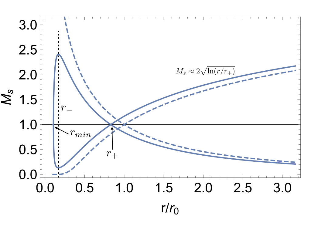
Figure 1: Phase diagram for Parker wind with rotation. Plotted is sonic Mach number $M_{s}$ versus radius normalized to Parker-Bondi radius $r_{0}$; parameter $R_{\Omega}=0.75r_{0}$. Dashed line is the conventional isothermal Parker wind. Most important modifications in the rotating case is that the solution cannot extend to $r\rightarrow 0$. The large-$r$ asymptotic is not affected much. The value of $r_{min}$ is plotted in Fig. 3; the Mach numbers at $r_{min}$ are plotted in Fig. 4, evolution of density is plotted in Fig. 6.

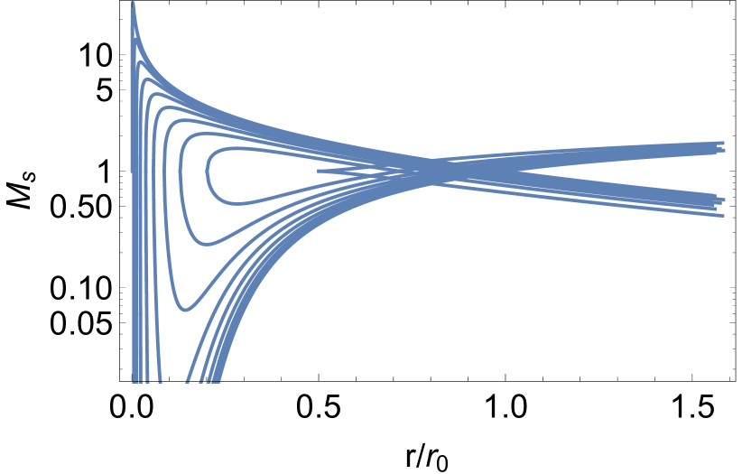
Figure 2: Same as Fig. 1 but for different $R_{\Omega}=0.1,0.2...1$.

General integral of (5) is (Bernoulli function)

$$B=\frac{M_{s}^{2}}{2}-\ln\left(M_{s}\right)-\frac{1}{2}\left(-\frac{R_{\Omega}^{2}}{2r^{2}}+\frac{4r_{0}}{r}+4\ln(r)\right)$$ (7)

The differential of the Bernoulli function vanishes only at $r_{+}$ - the only critical point in the flow.

The critical curves are given by

$$-\frac{M_{s}^{2}}{2}+\ln M_{s}=-\frac{1}{2}+\left(\frac{1}{r^{2}}-\frac{1}{r_{+}^{2}}\right)\frac{R_{\Omega}^{2}}{4}+2\left(\frac{1}{r_{+}}-\frac{1}{r}\right)r_{0}+2\ln\left(\frac{r_{+}}{r}\right)$$ (8)

Near the critical point $M_{s}=1,\,r=r_{+}$,

$$M_{s}=1\pm\sqrt{2-\frac{r_{0}}{r_{+}}}\left(1-\frac{r}{r_{+}}\right)$$ (9)

(the point $r_{0}=2r_{+}$ is when the critical point disappears).

At $r\gg r_{+}$ the Mach numbers evolve according to $M\approx 2\sqrt{\ln(r/r_{+})}$ for supersonic branch and $M\approx(r/r_{+})^{-2}$ for the subsonic branch, similar to the classical case of Parker wind.

The second point where the right hand side of Eq. (5) vanishes corresponds to points $r_{-}$, where $\partial_{r}M_{s}=0$. At the points $r_{-}$ the Mach number $M_{s}\neq 1$, see Fig. 4.

Finally, setting $M_{s}=1$ gives two roots: one is $r_{+}$ - the critical point of the flow; another defines the minimal $r_{min}$ for which the model is applicable

$$-\frac{R_{\Omega}^{2}}{4r_{\min}^{2}}-2\ln\left(\left(1+\sqrt{1-{R_{\Omega}^{2}}/{r_{0}^{2}}}\right)\frac{r_{0}}{2r_{\min}}\right)+\frac{2r_{0}}{r_{\min}}+\frac{R_{\Omega}^{2}}{r_{0}^{2}\left(1+\sqrt{1-\frac{R_{\Omega}^{2}}{r_{0}^{2}}}\right){}^{2}}-\frac{4}{1+\sqrt{1-\frac{R_{\Omega}^{2}}{r_{0}^{2}}}}=0,$$ (10)

see Fig. 3. At $r_{min}$ we have $\partial_{r}M_{s}=\infty$. So, neither $r_{-}$ or $r_{min}$ are critical points (the phase curve is smooth and non-self-intersecting at those points).

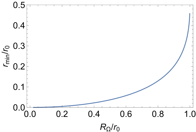
Figure 3: Value of $r_{min}$ for which the model is applicable as a function of $R_{\Omega}$. For $R_{\Omega}=0$ we have $r_{min}=0$, while for $R_{\Omega}=r_{0}$, $r_{min}=r_{0}/2$ and coincides at this moment with $r_{+}$.

For each given $R_{\Omega}$ the critical curve reaches at $r_{-}$ some maximal and minimal Mach numbers $M_{s,min/max}$, plotted in Fig. 4. Mach number at $r_{-}$ are not unity, except in the case $R_{\Omega}=r_{0}$, when points $r_{\pm}$ coincide.

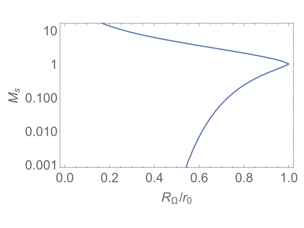
Figure 4: Maximal and minimal values of Mach number in the region $r\leq r_{+}$ along the critical curve as function of $R_{\Omega}$.

Overall phase diagrams are plotted in Fig. 5. For any $0<R_{\Omega}<r_{0}$ there are closed phase curves confined to $r_{min}<r<r_{+}$.

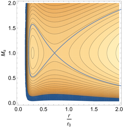
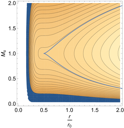
Figure 5: Phase curves on $r-M_{s}$ diagram for $R_{\Omega}=0.9r_{0}$ (left panel) and $R_{\Omega}=r_{0}$ (right panel). Critical curves are highlighted.

The density along the critical curves of Fig. 1 are plotted in Fig. 6.

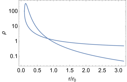
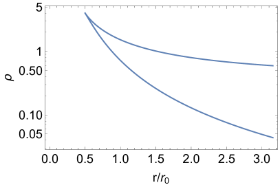
Figure 6: Density along the critical curves (plotted is the value of $r_{0}^{2}/(M_{s}r^{2})$) for $R_{\Omega}=0.75r_{0}$ and $R_{\Omega}=r_{0}$. At large radii larger densities correspond to the subsonic branch, where density reached a constant (since in that regime $M_{s}\propto r^{-2}$).

Given the velocity and density one can calculate the mass loss rate. It cannot be compared simply to the case of non-rotating winds. Usually, mass loss rate is calculated for a given base radius $R_{b}$ and local density - then the critical curve fixes the velocity. For rotating case, first, there is a limit on the radius $R_{b}>r_{min}$, so such a procedure may not work, and, second, the similar procedure will give some different launching velocity at the same radius.

3 Constraints on the parameters

3.1 Existence of the critical point

There are several constraints on the parameters. Let’s introduce two dimensionless parameters

$$\eta_{\Omega}=\frac{\Omega}{\Omega_{K}}\leq 1\mbox{}$$

$$\eta_{s}=\frac{c_{s}}{R_{b}\Omega_{K}}$$ (11)

where $\Omega_{K}$ is the break-up frequency at the equator. We find

$$\frac{R_{\Omega}}{r_{0}}=2\sqrt{2}\eta_{\Omega}\eta_{s}\mbox{}$$

$$c_{s}=\frac{\eta_{s}}{\sqrt{2}}v_{K}$$ (12)

where $v_{K}=\sqrt{2GM/r}$.

For the points $r_{\pm}$ to exist, it is required that $R_{\Omega}<r_{0}$, which translates to

$$\Omega\leq\Omega_{crit,1}=\frac{1}{2\sqrt{2}}\frac{GM}{c_{s}R_{b}^{2}}=\frac{1}{2\sqrt{2}}\frac{R_{b}\Omega_{K}^{2}}{c_{s}}=\frac{1}{2\sqrt{2}\eta_{s}}\Omega_{K}\mbox{}$$

$$2\sqrt{2}\eta_{\Omega}\eta_{s}\leq 1$$ (13)

Thus, there is a range $1/(2\sqrt{2})<\eta_{s}<1$ where $\Omega_{crit}<\Omega_{K}$. In physical units, this requires

$$c_{s}\geq\frac{1}{2\sqrt{2}}\sqrt{\frac{GM}{R_{b}}}$$ (14)

This is four times less that the escape velocity without rotation $\sqrt{2GM/R_{b}}$. Value (14) corresponds to the hydrodynamic energy parameter (HEP) of Waters & Proga (2012) $\lambda_{0}=GM/(R_{b}c_{s}^{2})=8$. For larger sound speed there is no critical point and the flow always remains supersonic or subsonic depending on the conditions at the launch location $R_{b}$.

For $R_{\Omega}=r_{0}$ we have

$$(1-M_{s}^{2})\frac{\partial_{r}M_{s}}{M_{s}}=-\frac{(2r-r_{0})^{2}}{2r^{3}}\mbox{}$$

$$\ln\left(M_{s}\right)-\frac{M_{s}^{2}}{2}=\frac{5}{2}+\frac{r_{0}^{2}}{4r_{\min}^{2}}-\frac{2r_{0}}{r_{\min}}+2\ln\left(\frac{r_{0}}{2r_{\min}}\right)$$ (15)

Thus, the numerator does not change sign - the outflow must start sonic at the critical point $r=r_{0}/2$. For larger $R_{\Omega}$ the wind must start supersonic outside of the critical point in order to be supersonic at infinity.

3.2 Connection to the base

The radius of the star $R_{b}$ cannot be smaller than $r_{min}$ for the model to be applicable. If the radius of the star $R_{b}$ is larger than $r_{-}$, then the wind continuously accelerate. The value of $r_{min}$ is very close to analytical $r_{-}$. The requirement $R_{b}\geq r_{-}$ translates to $\Omega<\Omega_{crit,2}$,

$$\Omega_{crit,2}=\sqrt{\Omega_{K}^{2}-2(c_{s}/R_{b})^{2}}\mbox{}$$

$$\frac{c_{s}}{R\Omega_{K}}\leq\frac{1}{\sqrt{2}}\sqrt{1-(\Omega/\Omega_{K})^{2}}$$ (16)

where $\Omega_{K}=\sqrt{GM_{\ast}/R_{b}^{3}}$ is Keplerian angular velocity at equator, see Fig. 7

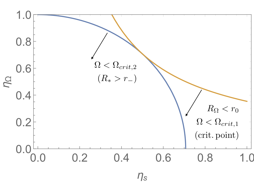
Figure 7: Allowed regions in the $\eta_{s}-\eta_{\Omega}$ plane.

There is also a special point where (13) and (16) match

$$\eta_{\Omega}=\frac{1}{\sqrt{2}}\mbox{}$$

$$\eta_{s}=\frac{1}{2}\mbox{}$$

$$R_{\Omega}=r_{0},\,\Omega_{max}=\Omega_{K}/2,\,r_{+}=r_{0}/2$$ (17)

In this case the wind starts sonically right from the surface $R_{b}$ and evolves according to

$$-\frac{M_{s}^{2}}{2}+\ln M_{s}=\frac{5}{2}-4\frac{R_{b}}{r}+\left(\frac{R_{b}}{r}\right)^{2}+2\ln\frac{R_{b}}{r}$$ (18)

3.3 Equatorial disk winds

One of the possible applications of the model is for thermal winds launched by disks (eg Weber & Davis, 1967; Konigl & Pudritz, 2000; Blandford & Payne, 1982; Waters & Proga, 2018). Assuming thin disk, so that the flow stars from a Keplerian-moving base, In this case then $\Omega=\Omega_{K}$, $\eta_{\Omega}=1$, $R_{b}$ means the local radius of the disk, and $c_{s}$ refers to the sound speed in the corona above the disk. Our parameters become

$$R_{\Omega}=\sqrt{2GM_{\ast}R_{b}}/c_{s}=2\sqrt{2}\eta_{s}r_{0}\mbox{}$$

$$\eta_{\Omega}=1\mbox{}$$

$$r_{+}=\frac{1}{2}\left(1+\sqrt{1-8\eta_{s}^{2}}\right)r_{0}$$ (19)

Thus, to have a critical point (to have a subsonic region) it is required that $\eta_{s}<1/(2\sqrt{2})=0.354$, or in physical units,

$$c_{s}\leq\frac{R_{b}\Omega_{K}}{2\sqrt{2}}=\frac{v_{K}}{4},$$ (20)

For larger coronal sound speed there is no critical point.

There is also the condition that $r_{min}$ should be smaller than $R_{b}$ for a flow to accelerate outwards. Here we cannot approximate $r_{min}$ as $\sim r_{-}$ (this would give only a trivial solution $\eta_{s}=0$). For the Keplerian disk $R_{b}=R^{2}_{\Omega}/(4r_{0})$ and, using the calculation of $r_{min}$, Fig. 3, we find that in order to start subsonically the coronal sounds speed should satisfy

$$\eta_{s}\leq 0.3190,$$ (21)

or, in physical units

$$c_{s}<0.3190R_{b}\Omega_{K}=0.225v_{K}$$ (22)

(for larger coronal sound speeds the critical curve does not reach a given point on the disk).

4 Discussion

In this paper we consider a highly idealized problem of thermal wind launched from a rotating object, a star or a disk. Our analytical results seem to be in agreement with previous numerical works by Skinner & Ostriker (2010); Waters & Proga (2012). In particular, Waters & Proga (2012) argued for a single critical point and also found regimes of non-continuous accelerations, “enthalpy deficit regime”.

Our results differ from the case of radiation-driven rotating winds (Friend & Abbott, 1986). In that case, e.g. the critical point moves outward due to rotation, while the terminal velocity is smaller. In our case the critical point moves inward, while at each radius the velocity is higher than in the non-rotating case. The critical conditions in line-driven winds are qualitatively different from the pressure-driven winds, (e.g. Lamers & Cassinelli, 1999).

It is of interest to discuss the cases of high rotation rates/high sound speeds when the model breaks down. There are two constraints: (i) connection to the base, $r_{min}\geq R_{b}$; (ii) existence of critical points, $R_{\Omega}<r_{0}$. If the condition (i) is broken, then the only way for a subsonic flow to connect to infinity is through unphysical “breeze” solution (it is subsonic, but typically has much larger pressure that prevents a smooth match to the interstellar medium). Similarly, if $R_{\Omega}>r_{0}$ and the flow is subsonic at the base, the breeze solution is the only choice. These cases are somewhat different from the classical Parker model, where the critical subsonic curve extends to $M_{s}=0$ as $r\rightarrow 0$. In our case all subsonic breeze solutions connect to supersonic non-critical solutions at $M_{s}=1$. In this regimes, most likely, the flow either becomes non-stationary and/or may form shocks.

The generalization to the polytropic case should be straightforward and follow the classic Parker’s case: instead of continuous acceleration, a supersonic branch of the flow would reach a constant velocity.

Appendix A Comparing with Skinner & Ostriker (2010) - Parker wind in cylindrical geometry

In cylindrical geometry Eq. (2) changes to

$$r\rho v_{r}={\rm Constant}$$ (A1)

while the wind equation becomes

$$\frac{v_{r}^{\prime}}{v_{r}}=\frac{c_{s}^{2}r^{2}+r^{3}\Phi^{\prime}(r)+R_{b}^{4}\Omega^{2}}{r^{3}(v_{r}^{2}-c_{s}^{2})}$$ (A2)

It differs from the spherical case, Eq. (4), only by a different factor ($1$ instead of $2$) in front of the $c_{s}^{2}$ term in the numerator. The structure of the equation remains the same, only with slightly changed definitions of the parameter (e.g., the location of critical points remain the same as (6) but with $r_{0}=GM/c_{s}^{2}$ and $R_{\Omega}=2R_{b}^{2}\Omega/c_{s}$).

References

- Blandford & Payne (1982) Blandford, R. D. & Payne, D. G. 1982, MNRAS, 199, 883
- Bondi (1952) Bondi, H. 1952, MNRAS, 112, 195
- Clarke & Alexander (2016) Clarke, C. J. & Alexander, R. D. 2016, MNRAS, 460, 3044
- Friend & Abbott (1986) Friend, D. B. & Abbott, D. C. 1986, ApJ, 311, 701
- Fukue & Okada (1990) Fukue, J. & Okada, R. 1990, PASJ, 42, 249
- Goossens (2003) Goossens, M., ed. 2003, Astrophysics and Space Science Library, Vol. 294, An introduction to plasma astrophysics and magnetohydrodynamics
- Keppens & Goedbloed (1999) Keppens, R. & Goedbloed, J. P. 1999, A&A, 343, 251
- Konigl & Pudritz (2000) Konigl, A. & Pudritz, R. E. 2000, Protostars and Planets IV, 759
- Lamers & Cassinelli (1999) Lamers, H. J. G. L. M. & Cassinelli, J. P. 1999, Introduction to Stellar Winds, 452
- Parker (1965) Parker, E. N. 1965, Space Sci. Rev., 4, 666
- Skinner & Ostriker (2010) Skinner, M. A. & Ostriker, E. C. 2010, ApJS, 188, 290
- Waters & Proga (2018) Waters, T. & Proga, D. 2018, MNRAS, 481, 2628
- Waters & Proga (2012) Waters, T. R. & Proga, D. 2012, MNRAS, 426, 2239
- Weber & Davis (1967) Weber, E. J. & Davis, L. J. 1967, ApJ, 148, 217