Quantitative estimates of chemical disequilibrium in Titan’s atmosphere
Abstract
We apply previously introduced measures of chemical disequilibrium to Cassini
mass spectroscopy data on the atmosphere of Titan. In the analysis presented here, we use
an improved description, avoiding the meanfield approximation in previous work.
The results of the analysis are nearly exactly the same as those found earlier
and confirm that, with respect to the measures used, Titan’s atmosphere lies between
living and many nonliving systems. Some details of the mathematical analysis, which
appear to be new, are included.
\draftfalse\journalname
JGR-Planets
School of Physics and Astronomy, University of Minnesota, Minneapolis, Minnesota, USA
\correspondingauthor
J. W. Halleyhalle001@umn.edu
{keypoints}
A nearly exact analysis of a statistical mechanical model for estimating
the degree of disequilibrium in Titan’s atmosphere is shown to agree with a previous
approximate analysis.
The estimated measures of disequilibrium of Titan’s atmosphere lie between those
of biological systems and some engineered polymer systems.
Some new features of the mathematical treatment of the model are described.
1 Introduction
The atmosphere of Titan has long been speculated
to have an atmosphere similar to that of early earth which might serve as a
model for prebiotic evolution(Clark et al, 1997; Trainer et al, 2006).
In the course of a recent study of data
on that atmosphere from
the NASA Cassini-Huygens mission to Saturn, we formulated (Intoy and Halley, 2018) an approximate model for
estimating how far that atmosphere is from
chemical equilibrium. The model took the form of a ferrimagnetic
Ising model for each of multiple linear chain molecules. In Intoy and Halley (2018) we made
an uncontrolled approximation, a kind of mean field theory, to determine the equilibrium
states of the model in analyzing the Titan data. Here we report a more exact analysis
which does not make that approximation.
Titan has a dense atmosphere made mostly of nitrogen.
Methane gas is present, with concentrations of about 2 atomic % (Waite et al, 2007),
which precipitates and cycles out of the atmosphere (Lunine et al, 2008).
as well as larger molecules up to 10,000 atomic mass units which were
detected in the
atmosphere on the mass spectrometer instruments of the Cassini spacecraft
(Waite et al, 2007). Mass spectrometry data are available for the negatively
charged, neutral and positively charged molecules in the atmosphere. The
most massive detected molecules were negatively charged.
The model presented here is intended to model the equilibrium distributions
of those larger molecules which are believed to be mainly composed of
nitrogen, carbon, and hydrogen. Although it is possible
that these large molecules could have complex structures,
we have assumed in the model that they are linear chains and we used
a ’united atom’ model in which the hydrogen entities are not treated explicitly.
An uncontrolled approximation for the partition function in the equilibrium description of the model reported here was
used in Intoy and Halley (2018) to estimate the degree to which the
atmosphere of Titan is out of local chemical equilibrium. and out
of chemical equilibrium with an external thermal bath at the
reported ambient temperature of that atmosphere.
Here we report details of an exact solution for the equilibrium partition
function of the model.
In the last section of the paper, we report results of the same
disequilibrium calculations described in Intoy and Halley (2018) using
the more exact equilibrium description given here.
In the next section, we describe the single chain model, its
extension to many chains, the way in which spatial dilution was
taken into account and the Gibbs limit of large negative chemical
potential which we will use in the analysis . In the third section
we describe calculations of
disequilibrium of Titan’s atmosphere like those reported in
our previous work Intoy and Halley (2018)
and compare the new results with those of those previous
approximate calculations.
2 Description of the Model
We consider a collection of linear chain molecules consisting of monomers
of two types, which we regard in the application as being ’united atom’ descriptions
of carbon and nitrogen plus some hydrogen atoms. Denoting the two entities as
C and N, and motivated by the C-C C-N and N-N bond energies reported from
first principles calculations in Table 1 we choose a model in which
those bond energies obey the relations
and . (In the numerical calculations reported in section
IV we used and . )
The relative concentration of monomers of the two types, which is known
experimentally (Crary et al, 2009) , is controlled in the model with
a magnetic field-like parameter .
Table 1: The average bond energies for carbon and nitrogen (Zumdahl, 2007).
Bond
Average Bond Energy (kJ/mol)
C-C
347
C-N
305
N-N
160
With those assumptions and that parametrization, the model for a single
chain with number of monomers takes the form of a
ferromagnetic one dimensional Ising model
(1)
where takes the values referring respectively to carbon and nitrogen monomers.
With the parametrization of the bond energies described above, the interaction matrix
takes the form
(2)
where .
controls the relative concentration of C and N as mentioned above.
The partition function is
(3)
where with the absolute temperature and Boltzmann’s constant.
Using the transfer matrix method (Kramers and Wannier, 1941) the exponential in equation 3
is factored into terms involving only two neighboring monomers:
(4)
where
(5)
Written out as a matrix, has the form:
(6)
In equation 2 the summations over
are matrix multiplications. The partition function is then
(7)
Since is a symmetric matrix there exists a unitary matrix , constructed from the
eigenvectors of , such that
, where is a diagonal
matrix containing the eigenvalues of .
Solving for the eigenvalues () and eigenvectors () yields:
(8)
(9)
where , , and are defined as
(10)
.Note that .
The matrix multiplication in equation 7
becomes
.
Where and since is unitary.
Substituting into equation 7 and summing over and gives:
(11)
(12)
(13)
(14)
Table 2:
for small values of using notation.
2
3
4
Table 3:
for small values of using notation. The case
where the magnetic field is zero (, ) is also shown.
2
3
4
Though contain a square root, it must be possible to express the as finite
polynomials in . We illustrate for small in tables
2 and 3.
More generally, can be written as
(15)
(16)
(17)
where is the number of states with energy .
could be calculated
by taking partial derivatives of the partition function in 14 with respect to , , and
, setting those respective variables to zero and comparing with 17
term by term giving
(18)
However, this method is computationally expensive for large systems. Instead we wrote the partition function in 14 in the form
17 by algebraic rearrangement as described in detail in
Appendix A with the result:
(19)
where
(20)
(21)
When , and the result for the partition function simplifies to
(22)
(23)
(24)
Where is the number of states with energy ,
(25)
and and retain the definitions in equation 10.
is shown for small values of in table 3.
is the number of configurations when only bonds are allowed.
A property of such configurations is that all sites with negative have sites
with positive
as neighbors. This property can be related to Fibonacci numbers
(Honsberger, 1985). The relation between and the
Fibonacci numbers is described in detail in appendix B.
For many Ising spin chains,
we assume that the
number of states associated with a single chain of energy is
. Here is the number of states with energy ,
is the number of places the chain
can be placed in volume , and
is the volume occupied by a polymer of length . We take
to be related to the persistence length (Intoy and Halley, 2018) () by
where is the polymer persistence length (Intoy and Halley, 2018) , is the bond length
and is a dimensionless index . We write this as with .
We used the value corresponding to random
walk behavior. (See also Intoy et al (2016) and Intoy and Halley (2018).)
A similar estimation for the number of states was used previously (Intoy et al, 2016).
The partition function for chains of length of which there are ,
where is the number of chains with energy , can be written as:
(26)
by an argument essentially identical to the one in reference Intoy et al (2016).
For a system of many polymers of various lengths, the partition function
becomes
or using the previous expression:
(27)
Denoting the total number of chains as we can then write the
grand canonical partition function as:
(28)
where the sum on in the last expression is unrestricted.
Expanding , then , and using the definition
that ,
we can move the summation over into the products with respect to , , and .
and also remove the restriction on the sum
yielding:
(29)
(30)
where in the last equality we used the identity
(31)
with
The Helmholtz free energy is then proportional to
(32)
where we denote , ,
and
The following quantities can then be calculated by taking partial derivatives
of equation 32:
Expected Total Number of Chains:
(33)
Expected Total Energy:
(34)
Expected Monomer Type Imbalance:
(35)
where is the total number of sites with respectively.
Note that when calculating the energy , and
are fixed (ie they are not regarded as dependent.)
That is because the energy of interest is only the energy associated with bonds and not
the energy associated with the chemical potential and the artificial magnetic field.
In equation 32 if the value of
is large and negative the following approximation, which we call the Gibbs limit,
can be used:
(36)
Then becomes:
(37)
(38)
(39)
Using this approximate form we have:
(40)
so that
Expected Number of Chains of length =
(41)
Expected Total Number of Monomers:
(42)
Expected Monomer Type Imbalance :
(43)
3 Application to Titan Data
Atmospheric data from Titan
(Desai et al, 2017) was analyzed to
extract a length distribution as described in Intoy and Halley (2018),
assuming that all the detected molecules were linear polymers.
To compare the length distributions inferred from the data with
the ones expected in equilibrium we established that the Gibbs limit
was a good approximation and used 41 rearranged as
(44)
where and
is the volume density of chains of length so that the total
density is .
An energy density can also be extracted
as described in Intoy and Halley (2018).
We then proceed as follows:
Set the experimentally determined number, energy densities and monomer type
imbalance to the equilibrium expressions and solve the resulting implicit
equations for and numerically with solutions
denoted . (We
used assuming that 2% of the monomers in the chains are
carbon (positive .) )Using those
values in the expression 41 gives what we call the local
equilibrium value
for each . The experimental values of the differ from these values
because the Titan atmosphere is not in local equilibrium. We measure the
degree to which it is out of local equilibrium by a normalized Euclidean distance
between
the local equilibrium point and the experimental point in the space of
populations of polymers of various lengths . The space has a
dimension of up to 104, though only values up to about are
numerically significant. Specifically
(45)
where is the length distribution of the data set.
We made a similar determination of an equilibrium point in the space corresponding
to equilibrium with an external heat bath with a fixed value. In that case,
we set the experimental values of the number density and the monomer imbalance
to their equilibrium expressions and solved the resulting implicit equations
for and numerically while leaving fixed.
(The value
T= degrees Kelvin (Crary et al, 2009) was used to fix .)
The resulting values of were then inserted
in the equilibrium expressions giving the coordinates of a point in the
space described by
We then evaluate a second normalized Euclidean distance from that equilibrium point,
termed the ’thermal’ equilibrium point as
(46)
where is the length distribution of the experimental data set.
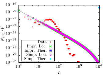
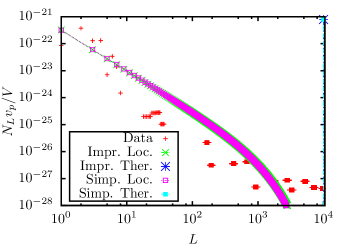
Figures 1-5
show the distributions of for various
altitude measurements and table 4
shows the numerical results for the parameters characterizing the local and
thermal equilibrium points.
Figure 1: values for the Titan atmosphere at an altitude of 1013km.
The data as well as the calculated improved (Impr.) and simple (Simp.)
local (Loc.) and thermal (Therm.) equilibria are shown.
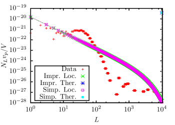
Figure 2: values for the Titan atmosphere at an altitude of 1032km.
The data as well as the calculated improved (Impr.) and simple (Simp.)
local (Loc.) and thermal (Therm.) equilibria are shown.
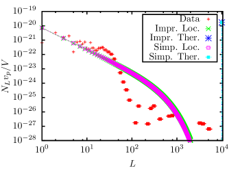
Figure 3: values for the Titan atmosphere at an altitude of 1078km.
The data as well as the calculated improved (Impr.) and simple (Simp.)
local (Loc.) and thermal (Therm.) equilibria are shown.
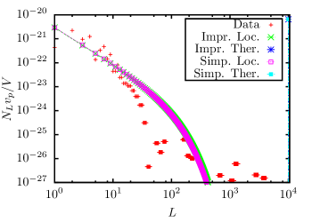
Figure 4: values for the Titan atmosphere at an altitude of 1148km.
The data as well as the calculated improved (Impr.) and simple (Simp.)
local (Loc.) and thermal (Therm.) equilibria are shown.
Figure 5: values for the Titan atmosphere at an altitude of 1244km.
The data as well as the calculated improved (Impr.) and simple (Simp.)
local (Loc.) and thermal (Therm.) equilibria are shown.
Table 4:
Values from the equilibrium calculations performed using the Titan
data and the resulting values of and .
Altitude (km)
Local
Local
Local
Thermal
Thermal
Thermal
4 Discussion and Conclusions
As one can see from the figures, the results of the improved
calculation of the partition function presented here are in excellent
agreement with the results of the simple mean field approximation
used in Intoy and Halley (2018). This appears to be mainly because the atomic
fraction of carbon in the application is very small (2%), making
corrections to a model with uniform bond strength small. It appears,
however that the lowest order corrections to the
limit in the two solutions are not the same. It would be interesting
to explore this aspect of the two approaches further.
Appendix A Calculations of .
Here we describe the algebraic rearrangement of equation 14 which gives the form closed form 17
for .
We consider a slightly different model in which
the magnetic field term
is defined as:
(47)
and then relate the coefficients of an expansion of the partition function in that
model to the coefficients in the original model.
Notice that counts the number of sites with .
Going through the same calculations described in section II yields the partition function and eigenvalues
(48)
(49)
where , (as in the main text) and
The eigenvalues and the partition function are different in the factors involving
the field because of the different field term.
Note that in 48 the RHS contains no radicals, whereas the middle equation contains radicals.
Secondly the RHS contains no denominator, so at some point the denominator is factored out
from the numerator.
In the following the binomial theorem is used frequently:
(50)
is rearranged as
(51)
(52)
and the eigenvalues as :
(53)
(54)
(55)
We then simplify by separating its non-radical and radical terms:
(56)
(57)
(58)
(59)
(60)
(61)
where:
(62)
(63)
(64)
(65)
We also simplify the terms in the square brackets in equation 52:
(66)
(67)
(68)
in this notation becomes:
(69)
(70)
(71)
(72)
(73)
and are rewritten to give a series in powers of , , and :
(74)
(75)
(76)
We rewrite this in terms of the summation variable instead of . The limits on the
summation on are somewhat complicated but we show that the the substitution
is justified because the extension of the limits
on only adds terms which are zero. The order of the sums on and is also
swapped
yielding the following form for
(77)
where
(78)
Similarly can be written as:
(79)
where:
(80)
These expressions for and are then inserted into equation 73 and the sums are rearranged
(81)
(82)
(83)
(84)
(85)
(86)
(87)
In going from the form (A38) to (A39) we introduced a change of summation
variable which changes the lower limit from to .
However the term with is zero and can be formally included.
By comparing powers of , , and we then have:
(88)
where it has been numerically verified that the coefficients of the
and terms are zero.
Finally we relate to the corresponding quantity in the original model
of the main text by relating the partition functions:
Let
(89)
(90)
which is the canonical form of the partition function of a spin system with
an external magnetic field as described in section II. Note that value of the term is the spin difference
which ranges from to in steps of 2 ().
Let
(91)
(92)
where now the term counts the number of positive spins which ranges from to .
To find a relation between and we rearrange :
(93)
(94)
Now let :
(96)
(97)
(98)
and can be written in the form:
(99)
(100)
where
(101)
By using the relation , (thus ) we relate and :
(102)
(103)
(104)
(105)
Therefore .
Appendix B Relation to Fibonacci Numbers
By setting and in equation 25 the eigenvalues can be rewritten as:
(106)
so that equals the golden ratio.
Consequently, a variety of identies can be used such as:
(107)
Manipulating equation 22 it can be related to the closed form solution of the Fibonacci numbers:
(108)
(109)
(110)
(111)
where is the th Fibonacci number.
Acknowledgements.
This work was supported by the United States National Aeronautics
and Space Administration (NASA) through grant NNX14AQ05G
and used the used the computational resources of
the University of Minnesota
School of Physics and Astronomy Condor cluster.
We thank Professor Gregg Musiker
in the math department for useful discussions and Ravindra Desai
for sharing his Titan data from Desai et al (2017).
The Titan data is available on NASA’s Planetary
Database System as well, in summary form in Desai et al (2017).
References
Clark et al (1997)
Clarke, David W and Ferris, James P in Planetary and Interstellar Processes Relevant to the Origins of Life, Springer-Verlag (1997),
pp 225-248
Trainer et al (2006)
Trainer, Melissa G and Pavlov, Alexander A and DeWitt, H Langley and Jimenez, Jose L and McKay, Christopher P and Toon, Owen B and Tolbert, Margeret A.,
Proceedings of the National Academy of Sciences 48, 18035 (2006)
Intoy and Halley (2018)
Intoy, B.F and Halley, J. W., http://biorxiv.org/cgi/content/short/327783v1
Waite et al (2007)
Waite, JH and Young, DT and Cravens, TE and Coates, AJ and Crary, FJ and Magee, B and Westlake, J, Science 316, 870 (2007)
Lunine et al (2008)
Lunine, Jonathan I and Atreya, Sushil K, Nature Geoscience 1, 159 (2008)
Crary et al (2009)
Crary, FJ and Magee, BA and Mandt, K and Waite Jr, JH and Westlake, J and Young, DT, Planetary and Space Science 57, 1847 (2009)
Zumdahl (2007)
Zumdahl SS and Zumdahl SA, Chemistry, Houghton Miflin Co. (2007) p.351
Kramers and Wannier (1941)
Kramers, HA and Wannier GH Phys. Rev. 60, 252 (1941)
Honsberger (1985)
Honsberger R, Mathematical Gems III,The Mathematical Association of America (1985), p.121
Intoy et al (2016)
Intoy, BF and Wynveen, A and Halley, JW, Physical Review E 94, 042424 (2016)
Desai et al (2017)
Desai, RT and Coates, AJ and Wellbrock, A and Vuitton, V and Crary, FJ and González-Caniulef, D and Shebanits, Oleg and Jones, GH and Lewis, GR and Waite, JH and others, The Astrophysical Journal 844, L18 (2017)