Quantifying the sensing power of crowd-sourced vehicle fleets

Sensors can measure air quality, traffic congestion, and other aspects of urban environments. The fine-grained diagnostic information they provide could help urban managers to monitor a city’s health lane2008urban ; cuff2008urban ; rashed2010remote ; dutta2009common . Recently, a ‘drive-by’ paradigm has been proposed in which sensors are deployed on third-party vehicles, enabling wide coverage at low cost driveby1 ; driveby2 ; driveby3 ; driveby4 . Research on drive-by sensing has mostly focused on sensor engineering driveby_network1 ; driveby_network2 ; driveby_data1 ; driveby_data2 ; driveby_data3 , but a key question remains unexplored: How many vehicles would be required to adequately scan a city? Here, we address this question by analyzing the sensing power of a taxi fleet. Taxis, being numerous in cities and typically equipped with some sensing technology (e.g. GPS), are natural hosts for the sensors. Our strategy is to view drive-by sensing as a spreading process, in which the area of sensed terrain expands as sensor-equipped taxis diffuse through a city’s streets. In tandem with a simple model for the movements of the taxis, this analogy lets us analytically determine the fraction of a city’s street network sensed by a fleet of taxis during a day. Our results agree with taxi data obtained from nine major cities, and reveal that a remarkably small number of taxis can scan a large number of streets. This finding appears to be universal, indicating its applicability to cities beyond those analyzed here. Moreover, because taxi motions combine randomness and regularity (passengers’ destinations being random, but the routes to them being deterministic), the spreading properties of taxi fleets are unusual; in stark contrast to random walks, the stationary densities of our taxi model obey Zipf’s law, consistent with the empirical taxi data. Our results have direct utility for town councilors, smart-city designers, and other urban decision makers.

Traditional approaches to urban sensing fall into two main categories (Fig. 1), each of which has limitations lane2008urban ; cuff2008urban ; rashed2010remote . At one extreme, airborne sensors such as satellites scan wide areas, but only during certain time windows. At the other extreme, stationary sensors collect data over long periods of time, but with limited spatial range. Drive-by sensing addresses the weakness in both these methods and offers good coverage in both space and time. In particular, mounting sensors on crowd-sourced urban vehicles, such as cars, taxis, buses, or trucks, enables them to scan the wide areas traversed by their hosts, allowing air pollution, road quality, and other urban metrics to be monitored at fine-scale spatiotemporal resolutions.

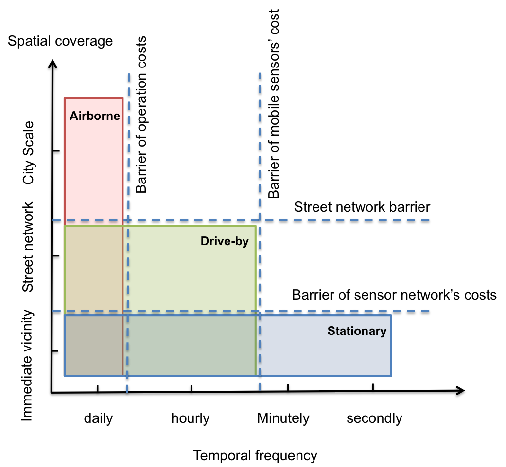
Figure 1: Comparison of different sensing methods. Airborne sensors, such as satellites, provide good spatial coverage, but their temporal coverage is limited to the time interval when the sensors pass over the location being sensed. Conversely, stationary sensors collect data for long periods of time, but have limited spatial range. Drive-by sensing offers some advantages of both methods. By utilizing host vehicles as ‘data mules,’ drive-by sensing offers a cheap, scalable, and sustainable way to accurately monitor cities in both space and time.

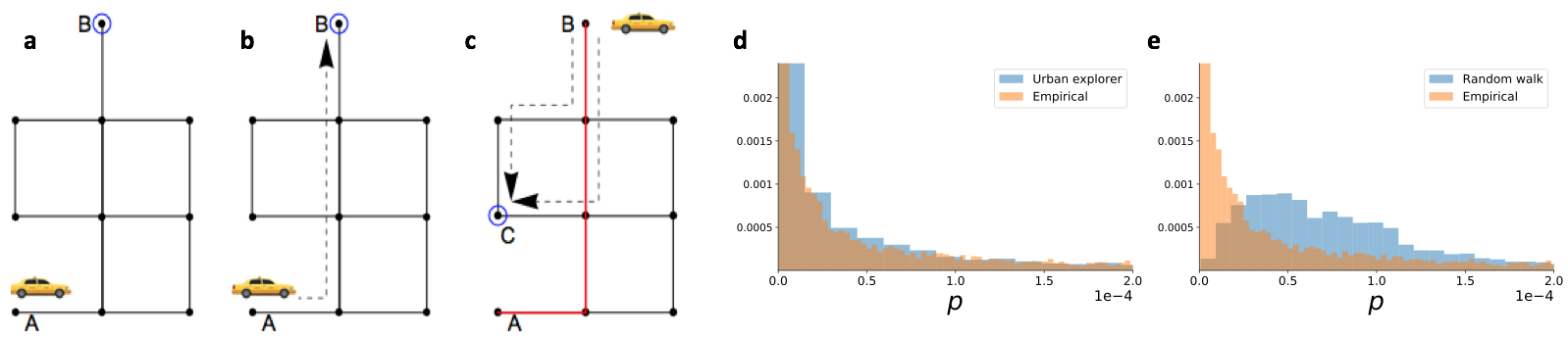
Figure 2: Urban explorer process. Panels (a)-(c) show a schematic of the urban explorer process. (a) A taxi picks up a passenger at node $A$. Then a destination node $B$ (blue circle) is randomly chosen. (b) The shortest path between $A$ and $B$ is taken (dashed arrow). No edges have yet been sensed. (c) After the edges connecting $A$ and $B$ have been traversed by the sensor-equipped taxi, they become ‘sensed,’ which we denote by coloring them red. Now at $B$, the taxi proceeds to its next pickup at, say, $C$. There are two shortest paths connecting $B$ and $C$, so one is chosen at random. This process then repeats. (d) Distribution of street segment popularities $p$ predicted by the urban explorer process (blue histogram) agree with empirical data from Manhattan (brown histogram). (e) By contrast, a random walk model of taxi movement incorrectly predicts a skewed, unimodal distribution of street segment popularities, in qualitative disagreement with the data. For panels (d) and (e) the (directed) Manhattan street network on which the urban explorer and random walk processes were run was obtained using the Python package ‘osmnx’. The urban explorer parameter $\beta$ was $1.5$, and the process was run for $T=10^{7}$ timesteps, after which the distribution of $p_{i}$ was observed to be stationary.

The power of drive-by sensing hinges on the mobility patterns of the host fleet; wide coverage requires the vehicles to densely explore a city’s spatiotemporal profile. We call the extent to which a vehicle fleet achieves this their sensing power. In what follows, we present a case study of the sensing power of taxi fleets.

Consider a fleet of sensor-equipped vehicles $\mathcal{V}$ moving through a city, sampling a reference quantity $X$ during a time period $\mathcal{T}$. We represent the city by a street network $S$, whose nodes represent possible passenger pickup and dropoff locations, and whose edges represent street segments potentially scannable by the vehicle fleet during $\mathcal{T}$. We use the proviso ‘potentially scannable’, since some segments are never traversed by taxis in our data sets and so are permanently out of reach of taxi-based sensing, as further discussed in Supplementary Note 1. To model the taxis’ movements we introduce the urban explorer process, a schematic of which is presented in Figs. 2(a)-(c). The model assumes that taxis travel to randomly chosen destinations via shortest paths, with ties between multiple shortest paths broken at random. Once a destination is reached, another destination is chosen, again at random, and the process repeats. To reflect heterogeneities in real passenger data, destinations in the urban explorer process are not chosen uniformly at random. Instead, previously visited nodes are chosen preferentially: the probability $q_{n}$ of selecting a node $n$ is proportional to $1+v_{n}^{\beta}$, where $v_{n}$ is the number of times node $n$ has been previously visited and $\beta$ is an adjustable parameter that depends on the city. This ‘preferential return’ mechanism is known to capture the statistical properties of human mobility song2010modelling , and as we show, also captures those of taxis.

To compare our model to data, we quantify the sensing power of a vehicle fleet as its covering fraction $\langle C\rangle$, defined as the average fraction of street segments in $S$ that are ‘covered’ or sensed by a taxi during time period $\mathcal{T}$, assuming that $N_{V}$ vehicles are selected uniformly at random from the vehicle fleet $\mathcal{V}$. (In Supplementary Note 5 we consider an alternate definition.)

We have computed $\langle C\rangle$ for 10 data sets from 9 cities: New York (confined to the borough of Manhattan), Chicago, Vienna, San Francisco, Singapore, Beijing, Changsha, Hangzhou, and Shanghai. (We used two independent data sets for Shanghai, one from 2014 and the other from 2015. For the 2015 data set, we chose the subset of taxi trips starting and ending in the subcity “Yangpu”, and hereafter consider it a separate city.) Each data set consists of a set of taxi trips. The representation of these trips differs, however, by city, and roughly falls into two categories. The Chinese cities comprise the first category, in which the GPS coordinates of each taxi’s trajectory were recorded, along with the identification (ID) number of the taxi. Knowing taxi IDs lets us calculate $\langle C\rangle$ explicitly as a function of the number of sensor-equipped vehicles $N_{V}$, as desired. Accordingly, we call these the “vehicle-level” data sets. For the remaining cities, however, trips were recorded without taxi IDs; in these cases we know only how many trips were taken, not how many taxis were in operation for the duration of our data sets. (Although taxi IDs are available for Yangpu and New York City, for reasons discussed in Supplementary Note 1 we exclude them from the vehicle-level data sets). So for these “trip-level” data sets we can only calculate the dependence of $\langle C\rangle$ on $N_{T}$, the number of trips, which serves as an indirect measure of the sensing power. Finally, since we represent cities by their street networks, and not as domains in continuous space, we map GPS coordinates to street segments using OpenStreetMap, so that trips are expressed by sequences of street segments $(S_{1},S_{2},\dots)$.

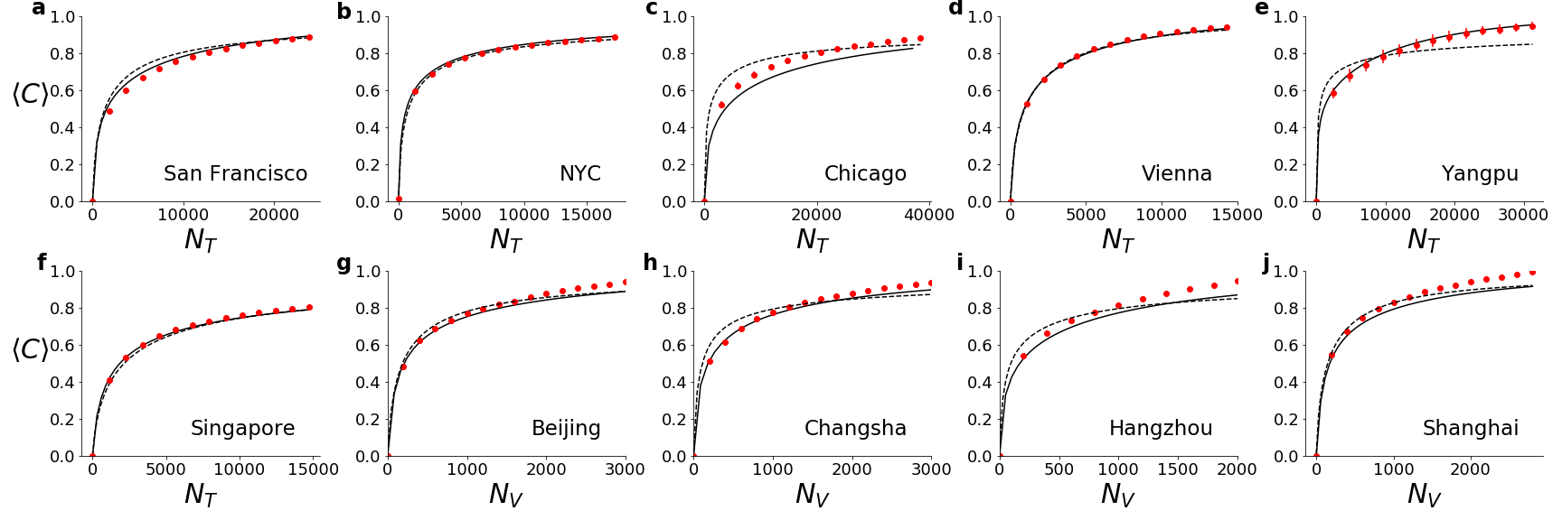
Figure 3: Sensing power $\mathbf{\langle C\rangle}$. Theoretical and empirical street-covering fractions $\langle C\rangle$ for all data sets. Panels (a)-(f) show the trip-level data, where the dependent variable is the number of trips $N_{T}$, and (g)-(j) show the vehicle-level data, where the dependent variable is the number of vehicles $N_{V}$. Thick and dashed curves show the analytic predictions for $\langle C\rangle$ using $p_{i}$ estimated from data and the urban explorer process respectively. Red dots show the empirical $\langle C\rangle$, whose calculation we describe in Supplementary Note 2. Notice in (a)-(f) the number of trips needed to scan half a city’s street segments, $N_{T}^{*}$, is remarkably low: $\sim 2000=10\%$, and in panels (g)-(j), $N_{V}^{*}\sim 5\%$. Exact figures for each $N_{T}^{*},N_{V}^{*}$ are given in Supplementary Note 4. We list the city name, date, and parameter $\beta$ for each city below: (a) San Francisco, 05/24/08, $\beta=0.25$ (b) New York City, 01/05/11, $\beta=1.5$ (c) Chicago, 05/21/14, $\beta=3.0$ (d) Vienna, 03/25/11, $\beta=0.25$ (e) Yangpu, 04/02/15, $\beta=2.75$ (f) Singapore, 02/16/11, $\beta=1.0$ (g) Beijing, 03/01/14, $\beta=1.0$ (h) Changsha, 03/01/14, $\beta=1.75$ (i) Hangzhou, 04/21/15, $\beta=1.25$ (j) Shanghai, 03/06/14, $\beta=0.75$.

We find that, despite its simplicity, the urban explorer process captures the statistical properties of real taxis’ movements. Specifically, it produces realistic distributions of segment popularities $p_{i}$, the relative number of times each street segment is sensed by the fleet $\mathcal{V}$ during $\mathcal{T}$ (in turn, these $p_{i}$ allow us to calculate our main target, $\langle C\rangle$). Figure 2(d) shows the empirical distribution of the $p_{i}$ obtained from our New York data set (brown histogram). The distribution is heavy tailed and follows Zipf’s law (this is also true of the other cities; see Supplementary Figure 2). The distribution predicted by the urban explorer process (blue histogram) is consistent with the data. This good agreement is surprising. One might expect the many factors absent from the urban explorer process – variations in street segment lengths and driving speeds, taxi-taxi interactions, human routing decisions, heterogeneities in passenger pickup and dropoff times and locations – would play a role in the statistical properties of real taxis. Yet our results show that, at the macroscopic level of segment popularity distributions, these complexities are unimportant. Moreover, the agreement of the model and the data is not trivial. Compare, for example, the predictions of a random walk model (Fig. 2(e)). With their skewed unimodal distribution, the random walk $p_{i}$ fail to capture the qualitative behavior observed in the data.

Having obtained the segment popularities $p_{i}$, we can predict the sensing power $\langle C\rangle_{N_{V}}$ analytically by using a simple ball-in-bin model. We treat street segments as ‘bins’ into which ‘balls’ are placed when they are traversed by a sensor-equipped taxi. Using the segment popularities $p_{i}$ as the bin probabilities, we derive (see Methods) the approximate expression

$$\langle C\rangle_{N_{V}}\approx 1-\frac{1}{N_{S}}\sum_{i=1}^{N_{S}}(1-p_{i})^{\langle B\rangle*N_{V}}.$$ (1)

Here $\langle B\rangle$ is the average distance (measured in segments) traveled by a taxi chosen randomly from $\mathcal{V}$ during $\mathcal{T}$. The ‘trip-level’ expression $\langle C\rangle_{N_{T}}$ is the same as Eq. (1) with $\langle B\rangle$ replaced by $\langle L\rangle$, the average number of segments in a randomly selected trip. (See Methods, Eq.(10).)

Figure 3 compares the analytic predictions for $\langle C\rangle$ against our data for a reference period of $\mathcal{T}=1$ day (see Supplementary Note 2 for how the empirical $C$ were calculated). We tested the prediction (1) in two ways: using $p_{i}$ estimated from our data sets (thick line), and using $p_{i}$ estimated from the stationary distribution of the urban explorer process (dashed line). In both cases theory agrees well with data, although the latter estimate is less accurate (as expected, it being derived from a model). Note that the $\langle C\rangle$ curves from different cities in Fig. 3 are strikingly similar. This similarity stems from the near-universal distributions of $p_{i}$ (shown in Supplementary Figure 1 and discussed in Supplementary Note 2) and suggests $\langle C\rangle$ might also be universal.

Figure 4 tests for universality in the $\langle C\rangle$ curves. Using the vehicle-level data, we rescale $N_{V}\rightarrow N_{V}/\langle B\rangle$, which removes the city-dependent term $\langle B\rangle$. (We assume the $p_{i}$ are universal, so we do not rescale them.) With no other adjustments, the resulting curves nearly coincide, as if collapsing on a single, universal curve. (The fidelity of the collapse however varies by day; see Supplementary Note 3). In Supplementary Figure 10 we perform the same rescaling for the trip-level data, which shows a poorer collapse. However since these data sets are of lower quality than the vehicle-level data, less trust should be placed in them. Hence, given the good collapse of the vehicle-level data, we conclude the sensing power of vehicle fleets, as encoded by $\langle C\rangle$, might be universal.

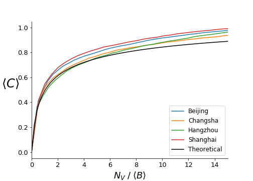
Figure 4: Scaling collapse. Empirical street-covering fractions $\langle C\rangle$ versus normalized number of sensor-equipped vehicles $N_{V}/\langle B\rangle$ from the four vehicle-level data sets. Remarkably, with no adjustable parameters, the curves for all four data sets fall close to the same curve, suggesting that at a statistical level, taxis cover street networks in a universal fashion. For each data set, the estimated values of $\langle C\rangle$ were found by drawing $N_{V}$ vehicles at random and computing the covering fractions. This process was repeated $10$ times. The variance in each realization was $O(10^{-3})$, so error bars were omitted. For the theoretical curve Eq. (1), the $p_{i}$ were estimated using the urban explorer process with $\beta=1.0$ on the Beijing street network. The choice of Beijing was arbitrary since, recall, the $p_{i}$ from different cities are nearly universal.

The fast saturation of the $\langle C\rangle$ curves tells us taxi fleets have large, but limited, sensing power; popular street segments are easily covered, but unpopular segments, being visited so rarely, are progressively more difficult to reach. A law of diminishing return is at play, which means that while scanning an entire city is difficult, a significant fraction can be scanned with relative ease. In particular, as detailed in Supplementary Note 4, about $65\%$ of vehicles are required to scan 80% of a city’s scannable street segments, but $50\%$ of segments are covered by just $N_{V}^{*}\sim 200\sim 5\%$ of vehicles (and at the trip level $N_{T}^{*}\sim 2000\sim 10\%$). Most strikingly, as shown in Supplementary Figure 11, one third of the street segments in Manhattan are sensed by as few as ten random taxis! In fact, because our estimates for $B$ are lower bounds (see Supplementary Note 2), the above quoted values for $N_{V}^{*}$ are likely lower. These remarkably small values of $N_{V}^{*}$ and $N_{T}^{*}$ are encouraging findings, and certify that drive-by sensing is readily feasible at the city scale, thus achieving the main goal of our work.

There are many ways to extend our results. To keep things simple, we characterized the sensing power of taxi fleets with respect to the simplest possible cover metric: the raw number of segments traversed by a taxi at least once, $C=\sum 1_{(M_{i}\geq 1)}$ (where as defined in Methods, $M_{i}$ is the number of times the $i$-th segment is sensed at the end of the reference period). A more general metric would be $C=\sum b_{i}1_{(M_{i}\geq 1)}$, where $b_{i}$ could represent the length of the segment or an effective sensing area. Also for simplicity, we confined our analysis to the fixed reference period of a day. This restriction could be relaxed by describing the segment popularities $p_{i}$ by a time-dependent Poisson process with densities estimated from data.

Taxis traveling in cities share some of the features of non-standard diffusive processes. Like Levy walks shlesinger1986levy ; blumen1989transport , or the run-and-tumble motion of bacteria schnitzer1993theory , their movements are partly regular and partly random. As such, they produce stationary densities on street networks that obey Zipf’s law, contrary to a standard random walk. Future work could examine if other aspects of taxis’ spreading behavior are also unusual. Perhaps the hybrid motion exemplified by taxis offers advantages in graph exploration tadic2003exploring , foraging viswanathan2011physics , and other classic applications of stochastic processes weiss1983random ; sp_physics2 .

The work most closely related to drive-by sensing is on ‘vehicle sensor networks’ van2017quality . Here, sensors capable of communicating with each other are fitted on vehicles, resulting in a dynamic network. The ability to share information enables more efficient, ‘cooperative’ sensing, but has the drawback of large operational cost. Most studies of vehicle sensor networks are therefore in silico gerla2012vehicular . Since the sensors used in drive-by sensing do not communicate, drive-by sensors are significantly cheaper to implement than vehicle sensor networks.

Vehicles other than taxis can be used for drive-by sensing. Candidates include private cars, trash trucks, or school buses. Since putting sensors on private cars might lead to privacy concerns, city-owned buses or trucks seem better choices for sensor hosts. The mobility patterns of school buses and trash trucks are however different to those of taxis; they follow fixed routes at fixed times, limiting their sensing power. The regularity in their motion opens up the possibility of ‘targeted sensing’. Should authorities want specific areas monitored at specific times, then sensors could be deployed on subsets of buses and trucks whose routes coincide with those sensing goals. This would yield more reliable coverage than that of taxis, whose random movements imply that sensing goals can only be probabilistically achieved. The downside of targeting sensing is that the spatiotemporal volume defined by the scheduled routes of trucks and buses is small compared to that of taxis. Therefore for wider, more homogeneous cover, taxis are the better choice of sensor host.

The diverse data supplied by drive-by sensing have broad utility. High-resolution air-quality readings can help combat pollution, while measurements of air temperature and humidity can help improve the calibration of meteorological models mead2013use ; katulski2010mobile and are useful in the detection of gas leaks murvay2012survey . Degraded road segments can be identified with accelerometer data, helping inform preventive repair nadeem2013mobile ; wang2014framework , while pedestrian density data can be helpful in the modeling of crowd dynamics kjaergaard2012mobile . Finally, information on parking-spot occupancy, WiFi access points, and street-light infrastructure – all obtainable with modern sensors – will enable advanced city analytics as well as facilitate the development of new big data and internet-of-things services and applications.

In short, drive-by sensing will empower urban leaders with rich streams of useful data. Our study reveals these to be obtainable with remarkably small numbers of sensors.

Methods

We wish derive an expression for the sensing power of a vehicle fleet. We quantify this by their covering fraction $\langle C\rangle_{N_{V}}$, the average fraction of street segments covered at least once when $N_{V}$ vehicles move on the street network $S$ according to the urban explorer process, during a reference period $\mathcal{T}$. Given the non-trivial topology of $S$ and the non-markovian nature of the urban explorer process, it is difficult to solve for $\langle C\rangle_{N_{V}}$ exactly. We can however derive a good approximation. It turns out that it is easier to first solve for the ‘trip-level’ $\langle C\rangle_{N_{T}}$ metric, that is, when $N_{T}$, the number of trips in the dependent variable, so we begin with this case (the ‘vehicle-level’ expression $\langle C\rangle_{N_{V}}$ then follows naturally).

Imagine we have a population $\mathcal{P}$ of taxi trajectories (defined, recall, as a sequence of street segments). The source of this population $\mathcal{P}$ is unimportant for now; it could come from a taxi (or fleet of taxis) moving according to the urban explorer process, or from empirical data, as we later discuss. Given $\mathcal{P}$, our strategy to find $\langle C\rangle_{N_{T}}$ is to map to a “ball-in-bin process”: we imagine street segments as bins into which balls are added when they are traversed by a trajectory taken from $\mathcal{P}$. Note that, in contrast to the traditional ball-in-bin process, a random number of balls are added at each step, since taxis trajectories have random length.

Trajectories with unit length. Let $L$ be the random length of a trajectory. The special case of $L=1$ is easily solved, because then drawing $N_{T}$ trips at random from $\mathcal{P}$ is equivalent to placing $N_{B}$ balls into $N_{S}$ bins, where $N_{S}$ is the number of segments, and each bin is selected with probability $p_{i}$. As indicated by the notation, we estimate these with the segment popularities discussed in the main text (we discuss this more later). Let $\vec{M}=(M_{1},M_{2},\dots,M_{N_{S}})$, where $M_{i}$ is the number of balls in the $i$-th bin. It is well known that the $M_{i}$ are multinomial random variables,

$$\vec{M}\sim\text{Multi}(N_{T},\vec{p})$$ (2)

where $\vec{p}=(p_{1},p_{2},\dots p_{N_{S}})$. The (random) fraction of segments covered is

$$C=\frac{1}{N_{S}}\sum_{i=1}^{N_{S}}1_{(M_{i}\geq 1)}$$ (3)

where $1_{A}$ represents the indicator function of random event $A$. The expectation of this quantity is

$$\langle C\rangle_{(N_{T},L=1)}=\frac{1}{N_{S}}\sum_{i=1}^{N_{S}}\mathbb{P}_{N_{T}}(M_{i}\geq 1)$$ (4)

(note we introduce $L$ as a subscript for explanatory purposes). The number of balls in each bin is binomially distributed $M_{i}\sim Bi(N_{B},p_{i})$. The which has survival function $\mathbb{P}(M_{i}\geq 1)=(1-(1-p_{i})^{N_{B}})$. Substituting this into (4) gives the result

$$\langle C\rangle_{(N_{B},L=1)}=1-\frac{1}{N_{S}}\sum_{i=1}^{N_{S}}(1-p_{i})^{N_{B}}.$$ (5)

Trajectories with fixed length. Trajectories of fixed (i.e. non-random) length $L>1$ impose spatial correlations between the bins $M_{i}$ (recall that in the classic ball and bin problem, the $M_{i}$ are already correlated, since their sum is constant and equal to the total number of balls added $N_{B}$). This is because trajectories are contiguous in space; a trajectory that covers a given segment is more likely to cover neighboring segments. Given the non-trivial topology of the street network $S$, the correlations between bins are hard to characterize. To get around this, we make the strong assumption that for $N_{T}\gg 1$ the spatial correlations between bins are asymptotically zero. This assumption greatly simplifies our analysis. It lets us re-imagine the ball-in-bin process so that adding a trajectory of length $L$ is equivalent to adding $L$ balls into non-contiguous bins chosen randomly according to $p_{i}$. Then, selecting $N_{T}$ trajectories of length $L$ from $\mathcal{P}$ is equivalent to throwing $N_{B}=L*N_{T}$ balls into $N_{S}$ bins $\langle C\rangle_{(N_{T},L_{fixed})}=\langle C\rangle_{(N_{T}*L,L=1)}$. Hence the expected coverage is a simple modification of (5):

$$\langle C\rangle_{(N_{B},L=1)}=1-\frac{1}{N_{S}}\sum_{i=1}^{N_{S}}(1-p_{i})^{L*N_{T}}.$$ (6)

Assuming neighboring segments are spatially uncorrelated is a drastic simplification, and effectively removes the spatial dimension from our model. Yet surprisingly, as we will show, it leads to predictions that agree well with data.

Trajectories with random lengths. Generalizing to random $L$ is straightforward. Let $S_{N_{T}}=\sum_{i=1}^{N_{T}}L_{i}$ be the number of segments covered by $N_{T}$ trajectories. By the law of total expectation

$$\langle C\rangle_{(N_{T},L)}=\sum_{n=0}^{\infty}\langle C\rangle_{(n,L_{fixed})}\mathbb{P}(S_{N_{T}}=n).$$ (7)

The first term in the summand is given by (6). For the second term we need to know how the trajectory lengths are distributed. In Supplementary Figure 4 we show $L\sim Lognormal(\tilde{\mu},\tilde{\sigma}^{2})$. It is known that a sum of lognormal random variables is itself approximately lognormal $S_{N_{T}}\sim Lognormal(\mu_{S},\sigma_{S}^{2})$, for some $\mu_{S}$ and $\sigma_{S}$. There are many different choices for $\mu_{S},\sigma_{S}$; for a review see lognormal . We follow the Fenton-Wilkinson method, in which $\sigma_{S}^{2}=\ln{(\frac{\exp{{\tilde{\sigma}^{2}}-1}}{N_{T}}+1)}$ and $\mu_{S}=\ln{(N_{T}\exp(\tilde{\mu}))}+(\tilde{\sigma}^{2}-\sigma_{S}^{2})/2$. Then,

$$\mathbb{P}(S_{N_{T}}=n)=\frac{1}{n\sigma_{S}\sqrt{2\pi}}e^{-\frac{(\ln{n}-\mu_{S})^{2}}{2\sigma_{S}^{2}}}.$$ (8)

Substituting this into (7) gives

$$\langle C\rangle_{(N_{T},L)}=\frac{1}{N_{S}n\sigma_{S}\sqrt{2\pi}}\sum_{n=0}^{\infty}\sum_{i=1}^{N_{S}}\big{(}1-(1-p_{i})^{n}\big{)}e^{-\frac{(\ln{n}-\mu_{S})^{2}}{2\sigma_{S}^{2}}}.$$ (9)

The above equation fully specifies the desired $\langle C\rangle_{(N_{T},L)}$. It turns out however that the sum over $n$ is dominated by its expectation, so we collapse it, replacing $n$ by its expected value $\langle L\rangle*N_{T}$. This yields the much simpler expression $\langle C\rangle_{(N_{T},L)}=\langle C\rangle_{(N_{T}*\langle L\rangle,L=1)}$, or

$$\langle C\rangle_{N_{T}}\approx 1-\frac{1}{N_{S}}\sum_{i=1}^{N_{S}}(1-p_{i})^{\langle L\rangle*N_{T}}$$ (10)

which appears in the main text.

Extension to vehicle level. Translating our analysis to the level of vehicles is straightforward. Let $B$ be the random number of segments that a random vehicle in $\mathcal{V}$ covers in the reference period $\mathcal{T}$ (in Supplementary Figure 4 we show how $B$ are distributed in our data sets). Then we simply replace $\langle L\rangle$ with $\langle B\rangle$ in the expression for $\langle C\rangle_{N_{T}}$ to get $\langle C\rangle_{N_{V}}$,

$$\langle C\rangle_{N_{V}}\approx 1-\frac{1}{N_{S}}\sum_{i=1}^{N_{S}}(1-p_{i})^{\langle B\rangle*N_{V}}.$$ (11)

Model parameters. The parameters $\langle L\rangle,\langle B\rangle$ in (11) as easily estimated from our data sets (see Supplementary Note 2). The bin probabilities $p_{i}$ are trickier. They have a clear definition in the ball-in-bin formalism, but in our model, the interpretation is not as clean; they represent the probability that a subunit of a trajectory taken at random from $\mathcal{P}$ covers the $i$-th segment $S_{i}$. As mentioned above, we estimate these with the segment popularities, which we calculate in two ways: (i) deriving them directly from our data sets; or (ii) from the urban explorer process (recall these methods led to similar distributions of $p_{i}$ as shown in Fig. 2(e)).

References

- (1) Lane, N. D., Eisenman, S. B., Musolesi, M., Miluzzo, E. & Campbell, A. T. Urban sensing systems: opportunistic or participatory? In Proceedings of the 9th workshop on Mobile computing systems and applications, 11–16 (ACM, 2008).
- (2) Cuff, D., Hansen, M. & Kang, J. Urban sensing: out of the woods. Communications of the ACM 51, 24–33 (2008).
- (3) Rashed, T. & Jürgens, C. Remote sensing of urban and suburban areas, vol. 10 (Springer Science & Business Media, 2010).
- (4) Dutta, P. et al. Common sense: participatory urban sensing using a network of handheld air quality monitors. In Proceedings of the 7th ACM conference on embedded networked sensor systems, 349–350 (ACM, 2009).
- (5) Lee, U. & Gerla, M. A survey of urban vehicular sensing platforms. Computer Networks 54, 4 (2010).
- (6) Hull, B. et al. Cartel: a distributed mobile sensor computing system. In Proceedings of the 4th international conference on Embedded networked sensor systems, 125–138 (2006).
- (7) Mohan, P., Padmanabhan, V. N. & Ramjee, R. Nericell: rich monitoring of road and traffic conditions using mobile smartphones. In Proceedings of the 6th ACM conference on Embedded network sensor systems, 323–336. (2008).
- (8) Anjomshoaa, A. et al. City scanner: Building and scheduling a mobile sensing platform for smart city services. IEEE Internet of Things Journal 1–1 (2018).
- (9) Skordylis, A. & Trigoni, N. Efficient data propagation in traffic-monitoring vehicular networks. IEEE Transactions on Intelligent Transportation Systems 12, 680–694 (2011).
- (10) Piran, M. J., Murthy, G. R., Babu, G. P. & Ahvar, E. Total gps-free localization protocol for vehicular ad hoc and sensor networks (vasnet). In Computational Intelligence, Modelling and Simulation (CIMSiM), 2011 Third International Conference on, 388–393 (2011).
- (11) Turcanu, I., Salvo, P., Baiocchi, A. & Cuomo, F. An integrated vanet-based data dissemination and collection protocol for complex urban scenarios. Ad Hoc Networks 52, 28–38 (2016).
- (12) Bridgelall, R. Precision bounds of pavement distress localization with connected vehicle sensors. Journal of Infrastructure Systems 21, 04014045 (2014).
- (13) Alessandroni, G. et al. Sensing road roughness via mobile devices: A study on speed influence. In Image and Signal Processing and Analysis (ISPA) (2015 9th International Symposium on. IEEE, 2015).
- (14) Song, C., Koren, T., Wang, P. & Barabási, A.-L. Modelling the scaling properties of human mobility. Nature Physics 6, 818 (2010).
- (15) Shlesinger, M. F., Klafter, J. & West, B. J. Levy walks with applications to turbulence and chaos. Physica A: Statistical Mechanics and its Applications 140, 212–218 (1986).
- (16) Blumen, A., Zumofen, G. & Klafter, J. Transport aspects in anomalous diffusion: Lévy walks. Physical Review A 40, 3964 (1989).
- (17) Schnitzer, M. J. Theory of continuum random walks and application to chemotaxis. Physical Review E 48, 2553 (1993).
- (18) Tadić, B. Exploring complex graphs by random walks. In AIP Conference Proceedings, vol. 661, 24–27 (AIP, 2003).
- (19) Viswanathan, G. M., Da Luz, M. G., Raposo, E. P. & Stanley, H. E. The physics of foraging: an introduction to random searches and biological encounters (Cambridge University Press, 2011).
- (20) Weiss, G. H. Random walks and their applications: Widely used as mathematical models, random walks play an important role in several areas of physics, chemistry, and biology. American Scientist 71, 65–71 (1983).
- (21) Ben-Avraham, D. & Havlin, S. Diffusion and reactions in fractals and disordered systems (Cambridge university press, 2000).
- (22) Van Le, D., Tham, C.-K. & Zhu, Y. Quality of information (qoi)-aware cooperative sensing in vehicular sensor networks. In Pervasive Computing and Communications Workshops (PerCom Workshops), 2017 IEEE International Conference on, 369–374 (IEEE, 2017).
- (23) Gerla, M., Weng, J.-T., Giordano, E. & Pau, G. Vehicular testbeds—validating models and protocols before large scale deployment. In Computing, Networking and Communications (ICNC), 2012 International Conference on, 665–669 (IEEE, 2012).
- (24) Mead, M. I. et al. The use of electrochemical sensors for monitoring urban air quality in low-cost, high-density networks. Atmospheric Environment 70, 186–203 (2013).
- (25) Katulski, R. J. et al. Mobile system for on-road measurements of air pollutants. Review of scientific instruments 81, 045104 (2010).
- (26) Murvay, P.-S. & Silea, I. A survey on gas leak detection and localization techniques. Journal of Loss Prevention in the Process Industries 25, 966–973 (2012).
- (27) Nadeem, T. M. & Loiacono, M. T. Mobile sensing for road safety, traffic management, and road maintenance (2013). US Patent 8,576,069.
- (28) Wang, M., Birken, R. & Shamsabadi, S. S. Framework and implementation of a continuous network-wide health monitoring system for roadways. In Nondestructive Characterization for Composite Materials, Aerospace Engineering, Civil Infrastructure, and Homeland Security 2014, vol. 9063, 90630H (International Society for Optics and Photonics, 2014).
- (29) Kjærgaard, M. B., Wirz, M., Roggen, D. & Tröster, G. Mobile sensing of pedestrian flocks in indoor environments using wifi signals. In Pervasive Computing and Communications (PerCom), 2012 IEEE International Conference on, 95–102 (IEEE, 2012).
- (30) Cobb, B. R., Rumi, R. & Salmerón, A. Approximating the distribution of a sum of log-normal random variables. Statistics and Computing 16, 293–308 (2012).