Estimation of a Heterogeneous Demand Function with Berkson Errors

Abstract

Berkson errors are commonplace in empirical microeconomics. In consumer demand this form of measurement error occurs when the price an individual pays is measured by the (weighted) average price paid by individuals in a specified group (e.g., a county), rather than the true transaction price. We show the importance of such measurement errors for the estimation of demand in a setting with nonseparable unobserved heterogeneity. We develop a consistent estimator using external information on the true distribution of prices. Examining the demand for gasoline in the U.S., we document substantial within-market price variability, and show that there are significant spatial differences in the magnitude of Berkson errors across regions of the U.S. Accounting for Berkson errors is found to be quantitatively important for estimating price effects and for welfare calculations. Imposing the Slutsky shape constraint greatly reduces the sensitivity to Berkson errors.

JEL: C14, C21, D12

Keywords: consumer demand, nonseparable models, quantile regression, measurement error, gasoline demand, Berkson errors.

1 Introduction

Datasets that are commonly used in microeconometric work often suffer from a particular type of measurement error in the covariates: Instead of observing the true covariate a household faces, the researcher observes a group-level (weighted) average, such as a regional average (e.g. in a county). The resulting errors in the covariate are called Berkson errors. Berkson measurement errors occur frequently in applied econometric analyses in which information on relevant covariates is not collected directly from households in a survey, but is taken from an alternative data source and assigned to households based on their location or other characteristics. While covariates assigned in this way will often be highly correlated with the true covariates, they will not be identical as long as there is some variability in the covariate within the specified group. For example, in the gasoline demand application discussed in Sections 5-6 of this paper, counties experience within-county price variability of up to 10 percent around the mean, and within-county variation accounts for a substantial share of the overall variation in prices. Furthermore, the amount of within-county price variability differs substantially across regions of the U.S., as shown in Figure 1 below.

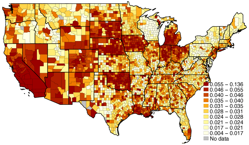
Figure 1: Within-market variability in gas prices across counties

Note: Map shows county-level standard-deviation in (log) gasoline prices (after removing county effects and day fixed effects). Based on station-level data from Yilmazkuday (2017), see Section 5.2 below for details.

Textbook analysis of this kind of econometric model often focuses on the case when the model is linear in the covariate and the error is additive. In this case, Berkson errors do not lead to a bias. This is sometimes taken to mean that Berkson errors are unlikely to cause significant bias in applied analysis, compared to say classical measurement error. However, these results no longer hold when the model is nonlinear. In nonlinear models, Berkson errors are not innocuous and require careful treatment.

In this paper we consider estimation of a demand model with nonseparable unobserved heterogeneity with Berkson errors. Consider the demand function with nonseparable unobserved heterogeneity

$$Q=G(P,Y,U)$$ (1)

where $Q$ is the quantity demanded, $P$ the price, $Y$ household income, and $U$ unobserved heterogeneity. Suppose now that we do not observe the true price at which a transaction took place, which we refer to as $P^{\star}$. Instead, we observe a county average price $P$ that is related to $P^{\star}$ by

$$P^{\star}=P+\epsilon,$$ (2)

where $\epsilon$ is an unobserved random variable, independent of $P$. With these Berkson errors (Berkson, 1950), the demand model becomes

$$Q=G(P+\epsilon,Y,U).$$ (3)

Importantly, Berkson errors in variables are different from classical errors in variables, where $P=P^{\star}+\epsilon$, with $\epsilon$ independent of $P^{\star}$.

In this paper, we argue that understanding the role of Berkson measurement errors in demand estimation is of growing relevance. The focus on understanding heterogeneity in responses motivates researchers to investigate behavior at different points in the distribution of unobserved heterogeneity, see e.g. Browning and Carro (2007). Moreover, researchers are increasingly interested in nonlinear models with non-separable unoberserved heterogeneity, see e.g. references in Cameron and Trivedi (2005); Blundell et al. (2012, 2017). Better data and increased computational power facilitate the study of models that do not impose linearity restrictions and, instead, allow flexible functional forms with a high degree of potential nonlinearity. Accordingly, nonlinear models are increasingly important in applications.

This paper develops a method for estimating a nonseparable demand model in the presence of Berkson errors, using a Maximum Likelihood Estimator (MLE) of quantiles of demand conditional on price and income. The standard quantile approach is inconsistent when prices are subject to Berkson errors. The maximum likelihood procedure we propose estimates all quantiles simultaneously, and a monotonicity constraint is used to ensure that the estimated quantiles do not cross. This estimator enables us to contrast the resulting estimates to results obtained assuming the absence of Berkson errors. Our estimation procedure accounts for spatial differences in the extent of Berkson error across locations, a feature which we find to be quantitatively important in our empirical application.

Delaigle et al. (2006) show the demand function is unidentified nonparametrically unless either the distribution of the Berkson error is known or can be estimated consistently from auxiliary data. Alternatively identification can be delivered if there is an instrument that is related to the true price in a suitable way (Schennach, 2013). We choose to follow the first of these approaches and use auxiliary data from external sources to inform us about the distribution of the Berkson error. We then assess the sensitivity to Berkson errors across different levels of the Berkson error variance. Finally, we note there is a potential for prices to be endogenous. To address this we develop a test for the exogeneity of covariates in the presence of Berkson errors.

We motivate and illustrate our analysis with an application to gasoline demand. Household travel surveys frequently assign gasoline prices from external sources based on the location of the household, leading to the presence of Berkson errors. A long-standing body of work has documented the importance of allowing for potential non-linearities in household gasoline demand (Hausman and Newey (1995); Yatchew and No (2001); Blundell et al. (2012)). The role of unobserved heterogeneity motivates a quantile modelling approach (Blundell et al. (2017); Hoderlein and Vanhems (2018)). These considerations suggest that nonlinearity plays an important role in this appliciation, highlighting the importance of Berkson errors in applied research and the need to treat them carefully.

We find that accounting for Berkson errors is quantitatively important. For example, Deadweight Loss measures derived from our estimates differ substantially when we allow for Berkson errors. In previous work we have investigated the role of shape restrictions in semiparametric or nonparametric estimation settings (Blundell et al. (2012, 2017)). In a setting with Berkson errors, we find that imposing shape restrictions, in the form of the Slutsky inequality, reduces the sensitivity of the estimates to the presence of Berkson errors.

The paper proceeds as follows. In the next section, we introduce Berkson errors and outline the demand model. Section 3 develops the MLE estimator. Section 4 presents the exogeneity test. In Section 5, we describe household gasoline data, and also document external evidence on the distribution of current local gasoline prices. The estimation results for the gasoline demand responses to prices and for deadweight loss welfare measures are presented in Section 6. Section 7 concludes.

2 Berkson Errors and the Demand Model

We begin this section by providing examples of where Berkson errors occur in applied microeconometric work. We then focus on Berkson errors in demand analysis; we outline the nonseparable demand model in the absence of Berkson errors, and then introduce Berkson errors into the model.

2.1 Examples of Berkson Errors

Berkson errors occur commonly in applied econometric work. Our application is to prices in consumer demand. Here we describe three additional examples where Berkson errors are likely to be relevant.

A common case is a situation where the researcher does not observe the true value of the variable of interest, but instead only observes an indicator for the group the individual belongs to. The researcher then assigns a ‘typical value’ from an external dataset, often the group average. This group will often be a geographic identifier or a time period. For example, relevant covariates may not be surveyed or measured at the level of the household, but are instead approximated by a regional average from an external source. For example, Currie and Neidell (2005) study the effect of air pollution on infant death in California. Since pollution measures are not available at the household level, exposure is measured for each zip code as a weighted average of all fixed pollution monitors installed within a given distance from the zip code centroid.

Another case is the situation where implementing a treatment exposes individuals to unobserved heterogeneity in the treatment intensity. In this setting, the intensity of a treatment varies randomly and in unobserved manner across treated units. This could be due to variability in the technology delivering the intervention, or due to differences in the staff implementing the treatment. For example, the dose of a drug delivered might vary slightly across patients, the amount of fertilizer spread on plots might vary randomly, or the support provided to unemployed workers might vary with the caseworker. For the latter case, Schiprowski (2019) documents significant variation in the effectiveness of caseworker meetings for unemployed workers, depending on the productivity of the caseworker; at the same time, details of the caseworker assigned to the unemployed are typically not observed by researchers.

A third case is a situation where individuals are uncertain about a relevant quantity and provide an optimal prediction (Hyslop and Imbens, 2001). For example, respondents in a survey are asked about a quantity they are uncertain about, and provide the best estimate of this quantity given their information set. When respondents provide an optimal prediction, the resulting prediction error is uncorrelated to the reported value. Phelps (1972) develops a model where firms infer productivity from a noisy signal as well as characteristics of the individual, and form an optimal prediction by a weighted average of the signal and the expected value given the characteristics. Due to the optimal prediction any deviation from the true value will be unrelated to the prediction made by the uncertain individual.

Survey data frequently asks respondents to provide details on variables where respondents may be uncertain about the exact values. For example, Chan and Stevens (2004) investigate how pension accumulations affect retirement decisions. Since data on pensions is self-reported in their data, the authors consider the possibility that the pension measure may be a noisy measure of the truth, predicted by the survey respondent, leading to Berkson error.

In another setting, Hastings et al. (2009) study benefits from attending higher achieving schools. They use Bayes’ rule to infer a parental preference parameter from a model of demand for schools, and in turn estimate models which allow the benefits of attendance to vary with this parental preference parameter. The measurement error in the estimated parental preference parameter then exhibits Berkson errors.

In all these cases, the variable used in the analysis differs from the variable which is relevant for the outcome in a way described by the Berkson error framework. This underscores the wide relevance of these kinds of measurement error for applied econometric work.

2.2 The Demand Model and the Presence of Berkson Errors

In the absence of Berkson errors, the demand function with nonseparable unobserved heterogeneity is set out in equation (1) in Section 1. We assume for now that $U$ is a scalar random variable that is statistically independent of $(P,Y)$, and that $G(P,Y,U)$ is monotone increasing in its third argument. We further assume without further loss of generality that $U\sim\text{U}[0,1]$.

Under these assumptions, the $\alpha$ quantile of $Q$ conditional on $(P,Y)$ is

$$Q_{\alpha}=G(P,Y,\alpha)\equiv G_{\alpha}(P,Y).$$

That is, the the conditional $\alpha$ quantile of $Q$ recovers the demand function $G$, evaluated at $U=\alpha$.

With Berkson errors, the demand model becomes equation (3). The function $G$ is unidentified nonparametrically unless either the distribution of $\epsilon$ is known or can be estimated consistently from auxiliary data (Delaigle et al. (2006)) or, alternatively, there is an instrument $Z$ that is related to the true price $P^{\star}$ in a suitable way (Schennach (2013)). In this work we follow the first of these approaches, and use auxiliary data to inform us about the distribution of the Berkson error.

3 Estimation

3.1 A Maximum Likelihood Estimator

In this section we develop the Maximum Likelihood Estimation approach. The model is

$$Q=G(P+\epsilon,Y,U);\;\;U\sim\text{U}[0,1].$$

Therefore,

$$P(Q\leq z|P,Y) =P(G(P+\epsilon,Y,U)\leq z|P,Y)=P(U\leq G^{-1}(P+\epsilon,Y,z)|P,Y)$$ (4)

$$=\int G^{-1}(P+\epsilon,Y,z)f_{\epsilon}(\epsilon)d\epsilon$$

$$=E_{\epsilon}G^{-1}(P+\epsilon,Y,z),$$

where $G^{-1}(\cdot,\cdot,z)$ is the inverse of $G$ in the third argument.

The left-hand term of equation (4), $P(Q\leq z|P,Y)$, is identified by the sampling process. $G^{-1}$ and $G$ are identified nonparametrically if and only if $G^{-1}$ is determined uniquely by

$$P(Q\leq z|P,Y)=E_{\epsilon}G^{-1}(P+\epsilon,Y,z).$$

This requires knowledge of $f_{\epsilon}(\epsilon)$; Delaigle et al. (2006) present a similar identification result for a conditional mean model.

The truncated series

$$G^{-1}(P+\epsilon,Y,Q)\approx\sum_{j=1}^{J}\theta_{j}\Psi_{j}(P+\epsilon,Y,Q)$$ (5)

provides a flexible parametric approximation to $G^{-1}$. In the truncated series, $J$ is the (fixed) truncation point, the $\Psi_{j}$ ’s are basis functions and the $\theta_{j}$ ’s are Fourier coefficients. The data ${\{Q_{i},P_{i},Y_{i}:i=1,...,n\}}$ are a random sample of $n$ households. The log-likelihood function for estimating parameter vector $\theta$ is the logarithm of the probability density of the data. This is:

$$\log L(\theta)=\sum_{i=1}^{n}log\sum_{j=1}^{J_{n}}\theta_{j}\int\left.\frac{\partial\Psi_{j}(P_{i}+\epsilon,Y_{i},z)}{\partial z}\right|_{z=Q_{i}}f_{\epsilon}(\epsilon)d\epsilon$$

Maximum likelihood estimation of $\theta$ consists of maximizing $\log L(\theta)$ subject to the following constraints: first, that $G^{-1}$ is non-decreasing in its third argument, and second, $0\leq G^{-1}\leq 1$. The maximum likelihood procedure estimates all quantiles simultaneously, and by imposing the monotonicity constraint above ensures that the estimated quantiles do not cross. For the presentation of the results, we numerically invert the estimated function $\hat{G}^{-1}$ to obtain the corresponding demand function $\hat{G}$.

3.2 Shape Restrictions

In some of the estimates we also impose the Slutsky shape restriction from consumer theory. Assuming quantity, income and prices for household $i$ are measured in logs, and $S_{i}$ reflects the budget share of household $i$, the Slutsky constraint, evaluated at $(P_{i},Y_{i},U_{i})$ can be written as

$$\frac{\partial Q}{\partial P}(P_{i},Y_{i},U_{i})+\frac{\partial Q}{\partial Y}(P_{i},Y_{i},U_{i})\;S_{i}\leq 0.$$

From $U=G^{-1}(P,Y,Q)$, we re-write the price and income effect in terms of $G^{-1}$, so that the Slutsky condition for household $i$ is

$$\frac{\partial G^{-1}}{\partial P}(P_{i},Y_{i},Q_{i})+\frac{\partial G^{-1}}{\partial Y}(P_{i},Y_{i},Q_{i})\;S_{i}\geq 0.$$ (6)

The estimation then proceeds by maximizing the log-likehood as before, adding the constraint (6) for a set of households in the data.

4 An Exogeneity Test

A common concern in demand estimation is the possible endogeneity of the price variable, where local prices are correlated with consumer preferences (see Blundell et al. (2012, 2017)). If a variable $W$ is available as an instrument for the price, the researcher can test for the presence of endogeneity. In a nonparametric or flexible parametric model, such a test is likely to have better power properties than a comparison of the exogenous estimate with an instrumental variables (IV) estimate. We therefore develop an exogeneity test, which takes account of the presence of Berkson errors. In this section we state the test statistic and asymptotic approximation to its distribution. The corresponding derivations can be found in Appendix A.2.

Assume that the instrument, $W$, satisfies

$$P(U\leq\tau|W,Y)=\tau.$$

Let $G^{-1}_{EX}$ denote the inverse demand function $G^{-1}$, described in Section 3, under the null hypothesis $H_{0}$ that $P$ is exogenous. Under $H_{0}$

$$\text{Pr}\left[G_{EX}^{-1}(P+\varepsilon,Y,Q|W=w,Y=y)\leq\tau\right]$$

$$=E\int I\left[G_{EX}^{-1}(P+\varepsilon,Y,Q|W=w,Y=y)\leq\tau\right]f_{\varepsilon}(\varepsilon)d\varepsilon=\tau$$ (7)

for any $(y,w)$ in the support of $(Y,W)$. The exogeneity test statistic is based on a sample analog of this relation. Let $f_{YW}$ denote the probability density function of $(Y,W)$. Let $K$ be a probability density function that is supported on $[-1,1]$ and symmetrical around 0. Let $\{h_{n}:n=1,2,...\}$ be a sequence of positive numbers that converges to 0 as $n\rightarrow\infty$. $K$ is called a kernel function and $\{h_{n}\}$ is called a sequence of bandwidths. Denote the data by $\{Q_{i},P_{i},Y_{i},W_{i}:i=1,\dots,n\}$. Let $\hat{f}_{YW}$ be a kernel nonparametric estimator of $f_{YW}$:

$$\hat{f}_{YW}(y,w)=\frac{1}{nh_{n}^{2}}\sum_{i=1}^{n}K\left(\frac{W_{i}-w}{h_{n}}\right)K\left(\frac{Y_{i}-y}{h_{n}}\right).$$

Let $\hat{G}^{-1}_{EX}$ denote the MLE of ${G}^{-1}_{EX}$. Define

$$S_{n}(y,w)= \frac{1}{nh^{2}}\sum_{i=1}^{n}\left\{\int I\left[\hat{G}_{EX}^{-1}(P_{i}+\varepsilon,Y_{i},Q_{i})\leq\tau\right]f_{\varepsilon}(\varepsilon)d\varepsilon K\left(\frac{W_{i}-w}{h_{n}}\right)K\left(\frac{Y_{i}-y}{h_{n}}\right)\right\}.$$

$S_{n}(y,w)/\hat{f}_{YW}(y,w)$ is a sample analog of the integral expression in (7). The test statistic is

$$T_{n}=nh_{n}^{2}\int\left[S_{n}(y,w)-\tau\hat{f}_{YW}(y,w)\right]^{2}dwdy.$$

To obtain an asymptotic approximation to the distribution of $T_{n}$, assume without loss of generality that $(y,w)\in[0,1]^{2}$. Let $\{\hat{\lambda}_{j}:j=1,\dots,n\}$ denote the eigenvalues of the operator

$$C(y_{1},w_{1};y_{2},w_{2})=\tau(1-\tau)\hat{f}_{YW}(y_{1},w_{1})\int K(\xi)K(\xi+\delta_{W})K(\zeta)K(\zeta+\delta_{Y})d\xi d\zeta.$$

Let $\{L_{n}:n=1,2,\dots\}$ be an increasing sequence of positive constants such that $L_{n}\rightarrow\infty$ and $n^{-1/2}L_{n}^{3/2}\rightarrow 0$ as $n\rightarrow\infty$. Under regularity conditions that are stated in the appendix,

$$\left|T_{n}-\sum_{j=1}^{L_{j}}\hat{\lambda}_{j}\chi^{2}_{j}\right|\rightarrow^{p}0$$

as $n\rightarrow\infty$, where the $\chi_{j}^{2}\;$s are independent random variables that are distributed as chi-square with one degree of freedom. The distribution of $T_{n}$ can be approximated by that of

$$\omega=\sum_{j=1}^{L_{n}}\hat{\lambda}_{j}\chi_{j}^{2}.$$

The quantiles of the distribution of $\omega$ can be estimated with any desired accuracy by Monte Carlo simulation.

5 Data on Demand and Prices

5.1 The household gasoline demand

The data are from the 2001 National Household Travel Survey (NHTS), which surveys the civilian noninstitutionalized population in the United States. This is a household level survey conducted by telephone, and complemented by travel diaries and odometer readings. These data provide information on the travel behavior of selected households. We focus on annual mileage by vehicles owned by the household.

In order to minimize heterogeneity in the sample, the following restrictions are imposed: We restrict attention to households with a white respondent, two or more adults, and at least one child under age 16. We drop households in the most rural areas, where farming activities are likely to be particularly important. We also omit households in Hawaii due to its different geographic situation compared to the continental states. Households without any drivers or where key variables are not observed are excluded, and we restrict attention to gasoline-based vehicles (excluding diesel, natural gas, or electricity based vehicles). The sample we use is the same as in Blundell et al. (2017).

A key aspect of the data is that although odometer readings and fuel efficiencies are recorded, price information is not collected at the household level, reflecting the expense in collecting purchase diaries and the resulting burden for respondents (EIA (2003); Leckey and Schipper (2011)). Instead, in the NHTS gasoline prices are assigned the fuel cost in the local area, based on the location of the household (EIA, 2003). In Section 5.2 we document that households face substantial price variability within local markets, and we use this information to assess the extent of Berkson errors.

The resulting sample contains 3,640 observations. Table 1 presents summary statistics.

Table 1: Sample descriptives

	Mean	St. dev.
		[t]
Log gasoline demand	7.127	0.646
Log price	0.286	0.057
Log income	11.054	0.580
		[b]
Observations	3640

Note: Table presents mean and standard deviations. See text for details.

The reported means of our key variables correspond to about 1,250 gallons of gasoline per year, a gasoline price of $1.33, and household income of about $63,000. For reference, Table 2 presents baseline estimates of price and income elasticities from a log-log model of gasoline demand.

Table 2: Log-log model estimates

	$\alpha=0.25$	$\alpha=0.50$	$\alpha=0.75$		OLS [t]
	(1)	(2)	(3)		(4) [b]
					[t]
$\log(p)$	-1.00	-0.72	-0.60		-0.83
	[0.22]	[0.19]	[0.22]		[0.18]
$\log(y)$	0.41	0.33	0.23		0.34
	[0.02]	[0.02]	[0.02]		[0.02]
Constant	2.58	3.74	5.15		3.62
	[0.25]	[0.21]	[0.25]		[0.20]
$N$	3640	3640	3640		3640

Note: Dependent variable is log gasoline demand. See text for details.

In the mean regression model, we find a price elasticity of -0.83 and an income elasticity of 0.34, similar to the elasticities reported in other studies of gasoline demand (see further Blundell et al. (2017)). Looking across quantiles, we find the lower quantile households to be more sensitive to changes in prices and income.

In the estimation below, the function $G^{-1}$ is specified as a product of three Chebyshev polynomials, one each for $P$, $Y$, and $Q$. We use cubic polynomials in price and income, and a 7th-degree polynomial in quantity. The high-degree polynomial in quantity enables us to estimate differences in the demand function across quantiles of the distribution of unobserved heterogeneity. When we impose the Slutsky constraint, using the observed data points in the sample, we restrict attention to those data points broadly in the areas of the data which we are focusing our analysis on below.

5.2 Dispersion in local gasoline prices

In this subsection, we present evidence on the within-market dispersion of gasoline prices. To gain insight into this, we draw on data collected by Yilmazkuday (2017), containing daily gas prices for virtually all gas station in the U.S. during a one-month period (July 2015) from MapQuest (http://gasprices.mapquest.com). Since these data are based on fleet transaction data, they are likely to be highly accurate. Together with the almost universal coverage of gas stations in these data, this dataset is very well suited for our purpose (see Yilmazkuday (2017) for further detail on these data).

To provide a description of the within-market price variability, Figure 2 shows a histogram of the gas prices (measured in logs), after removing county fixed effects and day fixed effects.

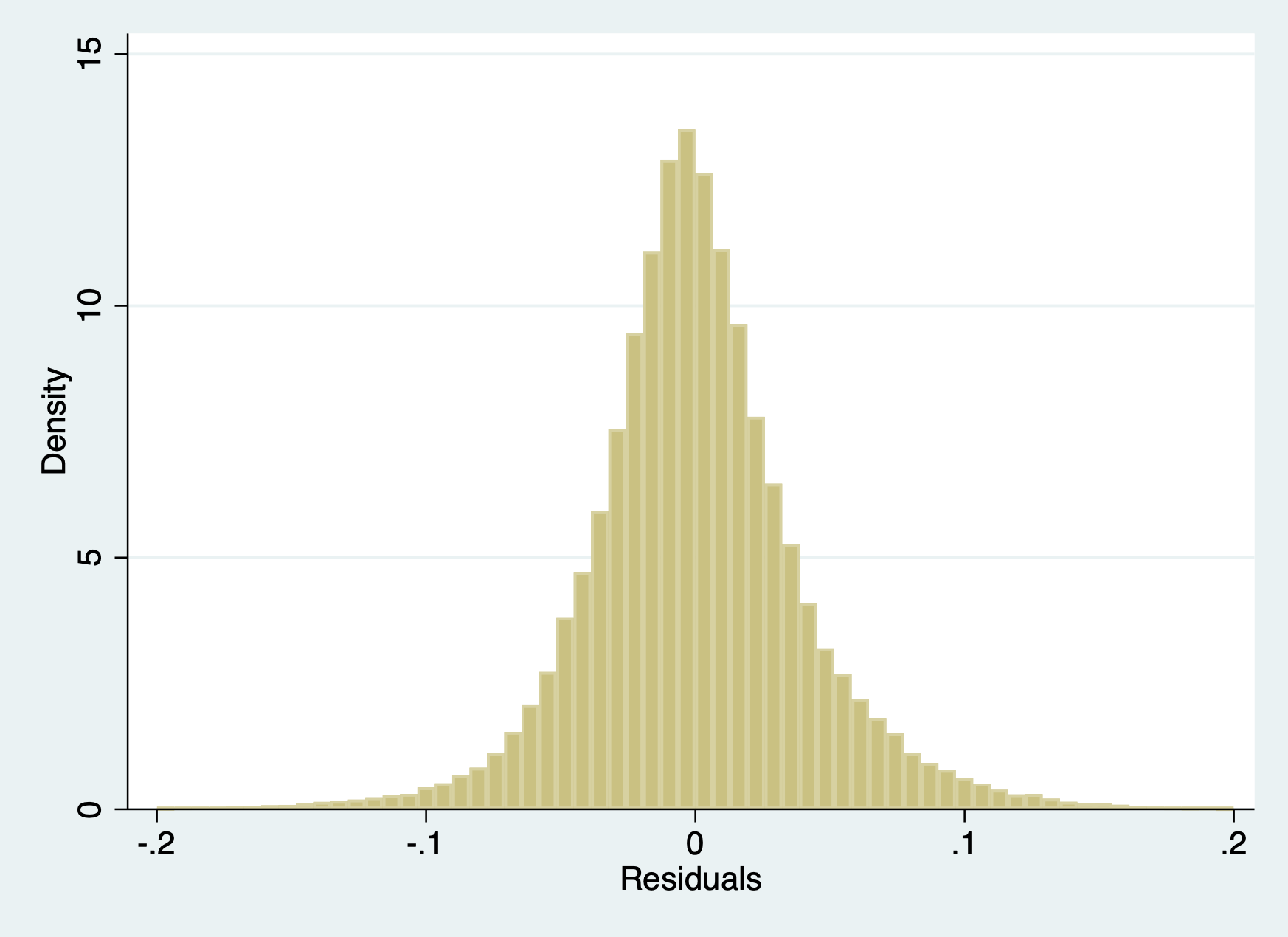
Figure 2: Within-market price distribution

Note: Histogram shows distribution of gasoline prices, after removing county effects and day fixed effects. See text for details.

This histogram shows that there is substantial within-market price variability. Within the same county (and having accounted for day effects), prices vary frequently by up to 10 percent in either direction. The histogram also suggests that a normal approximation of the within-market dispersion broadly captures the shape of the distribution.

To show the variability across counties in the price dispersion, we compute the within-county price dispersion for each county in the US. The resulting map is shown in Figure 1 above. As is evident from the map, price dispersion varies across the United States. For example, price variability is particularly high in California, but also in other states, such as Oklahoma, South Dakota or Nevada. Figure 3 shows the histogram of this within-county price dispersion.

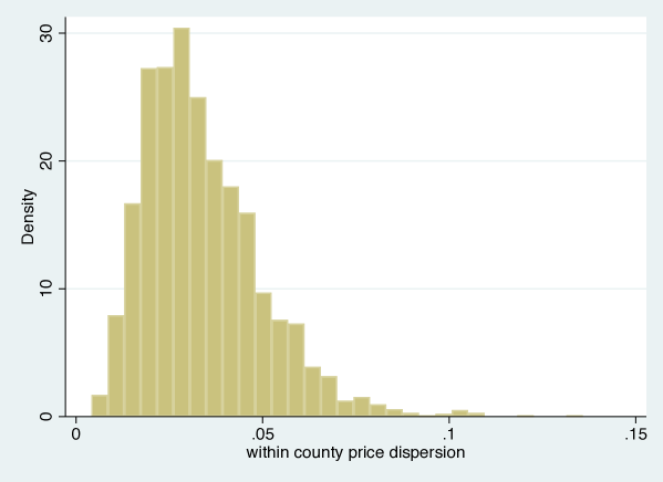
Figure 3: Variability in price distribution across counties

Note: Histogram shows distribution of county-level gas price dispersion, measured as standard deviation of (log) gasoline prices (after removing county effects and day fixed effects). See text for details.

Across all counties, the mean value (unweighted) of the within-market dispersion is 0.0339 (with first and third quartile taking values of 0.022 and 0.042). Comparing this value to the reported standard deviation of 0.057 in the NHTS price variable (see Table 1) shows that a significant amount of price variability occurs within local markets, suggesting that the Berkson error is an important feature of the price variation in this sample. In our empirical analysis, we use a normal distribution for the Berkson error, and allow the standard deviation to vary by U.S. state. To specify the standard deviation, we use a weighted average across the counties in each state (see Figure 1). This accounts for the substantial differences in the amount of Berkson errors across different parts of the U.S., and incorporates the spatial pattern of Berkson errors into our estimation.

5.3 Gasoline price cost shifter

To examine the exogeneity of prices we require a variable which is correlated with gasoline prices, but uncorrelated with the unobservable type of the household. Building on earlier work (Blundell et al., 2012), we use transportation cost as a cost shifter. This reflects that the cost of transporting the fuel from the supply source is an important determinant of prices.

We measure transportation cost with the distance between one of the major oil platforms in the Gulf of Mexico and the state capital. The U.S. Gulf Coast region accounts for the majority of total U.S. refinery net production of finished motor gasoline and for almost two-thirds of U.S. crude oil imports. It is also the starting point for most major gasoline pipelines. We therefore expect that transportation cost increases with distance to the Gulf of Mexico (see Blundell et al., 2012, for further details and references). Appendix Figure A.1 shows the systematic and positive relationship between state-level average prices and the distance to the Gulf of Mexico.

6 Empirical Results

6.1 Demand estimates

Figure 4: MLE estimates at the median (at middle income)

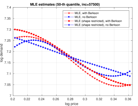
(a)

Note: The figure shows MLE estimates at the median ($\tau=0.50$) for the middle income group. Lines shown in red are estimates accounting for Berkson error, lines shown in blue assume absence of Berkson error. The figure compares unconstrained estimates versus Slutsky-constrained estimates (see legend). See text for details.

Figure 4 shows the ML estimates for the median, for the middle income group ($57,500). Figure 5 compares the estimates across the quartiles of the distribution of the unobserved heterogeneity, for the same income group.

Figure 5: MLE estimates across quartiles (at middle income)

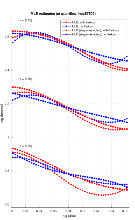
(a)

Note: The figure shows MLE estimates at the three quartiles (upper quartile, $\tau=0.75$, median, $\tau=0.50$, and lower quartile, $\tau=0.25$) for the middle income group. Lines shown in red are estimates accounting for Berkson error, lines shown in blue assume absence of Berkson error. The figure compares unconstrained estimates versus Slutsky-constrained estimates (see legend). See text for details.

The round markers show the MLE estimates without taking account of Berkson errors; the upside down triangular markers show the MLE with Berkson error. As can be seen from the Figure, accounting for Berkson errors accentuates the variability in the demand estimates, and leads to relevant differences in the estimated price responsiveness. For the median, for example, shifting the price across the full range shown in the figure (from 0.20 to 0.36) leads to a fall in estimated (log) demand by 0.11 assuming the absence of Berkson errors, compared to 0.21 in the presence of Berkson errors. Note the non-monotonicity in the unconstrained demand curve estimates, which is an artifact of random sampling variation (see further Blundell et al. (2012, 2017)). This non-monotonicity appears to accentuate the sensitivity to the Berkson errors in this empirical example.

The square markers in Figures 4 and 5 show the estimates when we impose Slutsky negativity. Although there is still a difference in the slope, the two sets of estimates are now much more similar. Looking across the different quantiles, we note a consistent finding that imposing the Slutsky inequality restriction removes non-monotonicity and delivers a smoother estimated demand curve much less sensitive to Berkson errors. This suggests that the estimates under the shape restriction are less sensitive to accounting for Berkson errors, reflecting the stabilizing effect of the shape restriction on the demand estimate.

Figure 6d compares the estimated effect at the median across the income distribution, comparing $72,500, $57,500, and $42,500, representing upper, middle and lower income households, respectively. These results highlight the importance of the Slutsky restriction in achieving monotonicity. In this way, these results not only provide demand function estimates that are consistent with consumer theory, but in addition attenuate sensitivity to Berkson errors. However, although the mitigation of sensitivity to Berkson errors through imposing the Slutsky restriction is a clear empirical finding of our analysis, we do not claim that it is a theoretical necessity.

Figure 6: MLE estimates across the income distribution (at $\tau=0.50$)

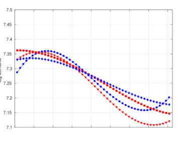
(a)

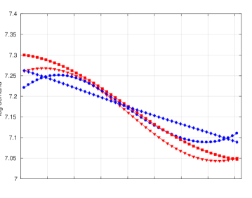
(b)

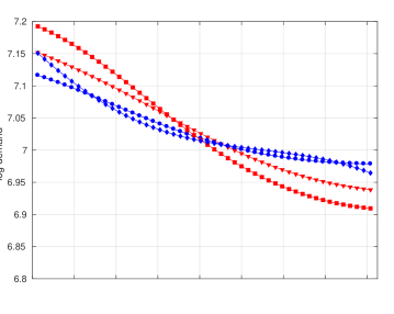
(c)

(d)

Note: The figure shows MLE estimates for the three income groups (top panel: ‘high’ income, corresponding to $72,500, middle panel: ‘medium’ income, corresponding to $57,500, and bottom panel: ‘low’ income, corresponding to $42,500) at the median ($\tau=0.50$). Lines shown in red are estimates accounting for Berkson error, lines shown in blue assume absence of Berkson error. The figure compares unconstrained estimates versus Slutsky-constrained estimates (see legend). See text for details.

Figure 7 compares the estimates for different magnitudes of the Berkson error, varying the standard deviation with factor 1.2 and factor 0.8, respectively. For small standard deviations (panel (b)), the presence of Berkson error makes very little difference to the demand estimates. However for larger standard deviation of the Berkson errors (panel (c)), the differences become quantitatively very important. This is especially pronounced for the unconstrained estimates.

Figure 7: Comparison of different magnitudes of the Berkson error

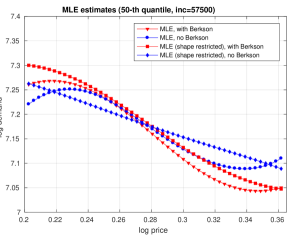
(a) factor 1

(b) factor 0.8

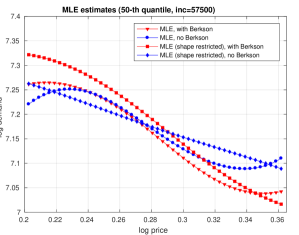
(c) factor 1.2

Note: The figure compares the baseline estimates in panel (a) to estimates with different standard deviation of the Berkson error. Panel (b) reduces the Berkson error standard deviation by factor 0.8, and panel (c) increases it by factor 1.2. Estimates shown for the median, at the middle income group. Lines shown in red are estimates accounting for Berkson error, lines shown in blue assume absence of Berkson error. Round markers indicate unconstrained estimates, square markers indicate Slutsky-constrained estimates. See text for details.

6.2 Estimating the welfare loss of gasoline taxation

The estimates of the demand function can be used to estimate welfare measures such as deadweight loss (DWL). We consider a hypothetical tax change which moves the price from $p^{0}$ to $p^{1}$ in a discrete fashion (see Blundell et al. (2017)). Let $e(p)$ denote the expenditure function at price $p$ and a reference utility level. The DWL of this price change is then given by

$$L(p^{0},p^{1})=e(p^{1})-e(p^{0})-(p^{1}-p^{0})\;H_{\alpha}\left[p^{1},e(p^{1})\right],$$

where ${H}_{\alpha}(p,y)$ is the Marshallian demand function. $L(p^{0},p^{1})$ is computed by replacing $e$ and $H$ with consistent estimates. The estimator of $e$, $\hat{e}$, is constructed by numerical solution of the differential equation

$$\frac{d\hat{e}(t)}{dt}=\hat{H}_{\alpha}\left[p(t),\hat{e}(t)\right]\frac{dp(t)}{dt},$$

where $\left[p(t),\hat{e}(t)\right]$ ($0\leq t\leq 1$) is a price-(estimated) expenditure path.

Deadweight Loss (DWL) estimates are reported in Table 3.

Table 3: DWL estimates

			with Berkson errors			without Berkson errors
			DWL per	DWL per		DWL per	DWL per
	income		tax	income		tax	income
			(1)	(2)		(3)	(4)
A. Upper quartile ($\tau$=0.75)
	high		0.155	7.82		0.054	3.00
unconstrained	middle		0.146	8.80		0.055	3.59
	low		0.116	8.70		0.043	3.34
	high		0.116	6.18		0.094	5.14
constrained	middle		0.140	8.52		0.093	5.92
	low		0.165	11.65		0.065	5.03
B. Median ($\tau$=0.50)
	high		0.130	4.70		0.061	2.40
unconstrained	middle		0.117	4.96		0.062	2.80
	low		0.101	5.17		0.052	2.80
	high		0.130	4.82		0.096	3.66
constrained	middle		0.139	5.90		0.092	4.04
	low		0.133	6.62		0.069	3.66
C. Lower quartile ($\tau$=0.25)
	high		0.087	2.20		0.077	2.03
unconstrained	middle		0.067	1.98		0.074	2.24
	low		0.064	2.28		0.069	2.50
	high		0.139	3.51		0.102	2.64
constrained	middle		0.118	3.48		0.094	2.80
	low		0.087	3.07		0.083	2.96

Note: DWL shown corresponds to a price change from the 5th to the 95th percentile in the data. Income level ‘high’ corresponds to $72,500, ‘medium’ to $57,500, and ‘low’ to $42,500. ‘DWL per income’ is re-scaled by $\times 10^{4}$ for readibility.

Looking at the unconstrained estimates, the table shows the strong quantitative difference in the DWL figures between the estimates with Berkson error (columns (1)-(2)) versus those without (columns (3)-(4)). In many cases, the estimates with Berkson errors but not the Slutsky restriction are more than twice as large as those assuming absence of Berkson errors.

Regarding the constrained estimates, however, the DWL figures are now much closer together and often of similar order of magnitude. This underlines a key point from the demand curve estimates in the previous subsection, the Slutsky constrained demand estimates reduce sensitivity to the presence of Berkson errors.

6.3 Exogeneity test

In this section we report the empirical results for the endogeneity test. To simplify the computation, we implement the univariate version of the test and specify a common standard deviation of the Berkson error distribution across the U.S. For this purpose, we stratify the sample along the income dimension in three groups: a low-income group of households (household income between $35,000 and $50,000), a middle-income group of households (between $50,000 and $65,000), and an upper-income group of households (between $65,000 and $80,000). The test is then performed for each income group. The results are shown in Table 4.

We find we do not reject exogeneity for any of the three income groups. This conclusion remains unchanged when we consider moderate variation in the extent of the Berkson error, multiplying the standard error of the Berkson error by a factor of 0.8 and 1.2, respectively, as shown in the table. The critical values shown in the table do not take account of the fact that we perform the test three times (for each of the three income groups). One possibility for adjusting the size for a joint 0.05 level test would be a Bonferroni adjustment. The adjusted $p$-value for a joint 0.05 level test of exogeneity is $1-(0.95)^{(1/3)}=0.01695$, at each of the three income groups. Using this more conservative cutoff would strengthen our conclusion. Based on these results, endogeneity is unlikely to be a first-order issue for our estimates.

Table 4: Exogeneity test

	test statistic	crit value (5%)	p-value	reject?
(a) HIGH INCOME (N=578)
baseline case	0.1575	0.4000	0.4490	no
reduced Berkson error, factor 0.8	0.1629	0.4000	0.4291	no
increased Berkson error, factor 1.2	0.1443	0.4000	0.5009	no
(b) MEDIUM INCOME (N=555)
baseline case	0.2257	0.4033	0.2459	no
reduced Berkson error, factor 0.8	0.1879	0.4033	0.3444	no
increased Berkson error, factor 1.2	0.2617	0.4033	0.1781	no
(c) LOW INCOME (N=580)
baseline case	0.1338	0.4042	0.5427	no
reduced Berkson error, factor 0.8	0.1490	0.4042	0.4799	no
increased Berkson error, factor 1.2	0.1777	0.4042	0.3768	no

Note: Income range ‘high’ refers to $65,000-$80,000, ‘medium’ to $50,000-$65,000, ‘low’ to $35,000-$50,000. Exogeneity test is conducted separately for each income range. Bonferroni-adjusted $p$-value for a joint 0.05 level test of exogeneity is $0.01695$. See text for details.

7 Conclusions

It has long been understood that in a mean regression model with a linear effect of a covariate with Berkson errors and an additive error term, the coefficients in an OLS regression are unbiased. Recent advances in methods, data, as well as computational capacity, together with a desire for understanding the effect of heterogeneity in the studied population, have led to a growing interest in nonlinear models. In nonlinear models, the role of Berkson errors is much less well understood, and ignoring these errors in general leads to a bias in the estimates. This motivates our interest in investigating the effect of Berkson errors, and methods for addressing their presence in the data. We conduct this analysis in the context of a quantile regression model, where the covariates enter through a flexible parametric specification, allowing for potential nonlinearity in the effects. Our application of interest is a gasoline demand model with unobserved heterogeneity, where the price is measured with Berkson error.

The presence of Berkson errors is a frequent feature of economic data. It occurs, for example, when the covariate is measured as a regionally aggregated average, masking within-region variability. The data generating process features the covariate which includes the Berkson error but its error-free value is unobserved by the researcher. This naturally raises the question how much difference recognizing the presence of Berkson error may make.

We derive a maximum likelihood estimator, which enables us to carry out consistent estimation in the presence of Berkson errors with a known density. The paper also develops a test for exogeneity of the Berkson covariate in the presence of an instrument.

We apply the method to the demand for gasoline in the U.S. We examine demand curves in which we impose the Slutsky inequality constraint and those that do not. The unconstrained estimated demand function display non-monotonicity in the price of gasoline. This estimated demand function is substantially affected by Berkson errors. The estimates which do not take account of the Berkson errors understate the variability in the price effect. These results show that accounting for Berkson error can have a substantial effect on the estimated demand function in a standard demand application. In turn, these estimates result in differences in DWL estimates for given price changes. In a number of cases, the DWL estimates recognizing the presence of Berkson errors are more than twice as large as estimates assuming the absence of Berkson errors. Thus, Berkson errors can have quantitatively large effects.

In our application, the estimated demand function is weakly non-monotonic in the price. As Blundell et al. (2012, 2017) explain, this can be due to the effects of random sampling errors on the estimate. We overcome this problem by imposing the Slutsky constraint on the structural demand function estimates, as a way of adding structure to the estimation problem. When the Slutsky restriction is imposed, the estimated demand function is well-behaved and the effects of Berkson errors are somewhat attenuated. These results illustrate that in a setting where measurement error increases the uncertainty of the estimates, shape restrictions such as the Slutsky constraint can be particularly useful for providing additional structure to improve the estimation.

Appendix A Appendix

A.1 Additional Tables and Figures

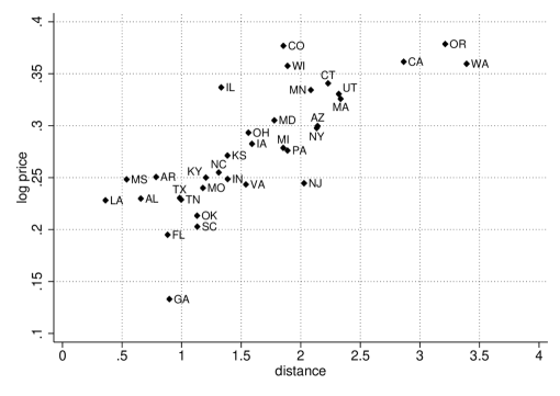
Figure A.1: Instrumental Variable for Price: Distance to the Gulf of Mexico

Note: Price of gasoline and distance to the Gulf of Mexico. Distance to the respective state capital is measured in 1000 km. Source: BHP (2012, Figure 5).

Table A.1: DWL estimates with confidence intervals

			with Berkson errors			without Berkson errors
			DWL per	DWL per		DWL per	DWL per
	income		tax	income		tax	income
			(1)	(2)		(3)	(4)
A. Upper quartile ($\tau$=0.75)
	high		0.155	7.81		0.054	3.00
			[ 0.101; 0.272]	[ 5.44; 13.58]		[ -0.016; 0.103]	[ -0.51; 5.76]
	middle		0.146	8.80		0.055	3.59
			[ 0.085; 0.238]	[ 5.66; 13.99]		[ -0.005; 0.105]	[ -0.00; 6.87]
	low		0.116	8.70		0.043	3.34
			[ 0.009; 0.205]	[ 1.74; 15.25]		[ -0.024; 0.123]	[ -1.51; 9.79]
B. Median ($\tau$=0.50)
	high		0.130	4.70		0.061	2.40
			[ 0.046; 0.224]	[ 1.99; 7.93]		[ -0.001; 0.114]	[ 0.18; 4.44]
	middle		0.117	4.96		0.062	2.79
			[ 0.045; 0.187]	[ 2.22; 7.81]		[ 0.010; 0.121]	[ 0.56; 5.46]
	low		0.101	5.17		0.052	2.80
			[ -0.005; 0.177]	[ 0.40; 9.00]		[ -0.015; 0.132]	[ -0.52; 7.20]
C. Lower quartile ($\tau$=0.25)
	high		0.087	2.20		0.077	2.03
			[ -0.027; 0.170]	[ -0.41; 4.27]		[ 0.012; 0.151]	[ 0.48; 3.98]
	middle		0.067	1.98		0.074	2.24
			[ -0.031; 0.124]	[ -0.71; 3.66]		[ 0.017; 0.147]	[ 0.69; 4.48]
	low		0.064	2.27		0.069	2.50
			[ -0.073; 0.138]	[ -2.03; 4.96]		[ -0.023; 0.157]	[ -0.36; 5.75]

Note: Table shows unconstrained DWL estimates with 90% confidence intervals, based on 499 bootstrap replications. DWL shown corresponds to a price change from the 5th to the 95th percentile in the data. Income level ‘high’ corresponds to $72,500, ‘medium’ to $57,500, and ‘low’ to $42,500. ‘DWL per income’ is re-scaled by $\times 10^{4}$ for readibility. See text for details.

A.2 Exogeneity Test

The argument that follows uses linear functional notation. In this notation,

$$Pg=\int gdP;\;\;\;P_{n}g=\int gdP_{n}$$

for any function $g(\cdot)$, where $P$ and $P_{n}$, respectively, are the distribution and empirical distribution functions of the random argument of $g$.

To obtain an asymptotic approximation to the distribution of $T_{n}$, make:

Assumption 1.

1. $G^{-1}_{EX}$ is a known bounded function $g(\cdot,\cdot,\cdot,\theta)$, where $\theta\in\mathbb{R}^{d}$ for some $d<\infty$ is a constant parameter whose maximum likelihood estimate is denoted by $\hat{\theta}$ and whose true but unknown population value is denoted by $\theta_{0}$.

2. $n^{1/2}\left(\hat{\theta}-\theta_{0}\right)\rightarrow^{d}N(0,V)$ for some non-singular covariance matrix $V$.

3. The first and second derivatives of $g$ with respect to its third argument are bounded and continuous uniformly over $\theta$ in a neighborhood of $\theta_{0}$ and the other arguments of $g$.

Assumption 2.

1. $K$ is a probability density function that is symmetrical about 0 and supported on $[-1,1]$.

2. $n^{1/2}h/(\log n)^{\gamma}\rightarrow\infty$ as $n\rightarrow\infty$ for some $\gamma>1/2$.

Define

$$G^{-1}_{EX}(\cdot,\cdot,\cdot)=g(\cdot,\cdot,\cdot,\theta).$$

Define

$$R_{n}(y,w,\varepsilon)= \frac{1}{nh^{2}}\sum_{i=1}^{n}I\left[\hat{G}^{-1}_{EX}\left(P_{i}+\varepsilon,Y_{i},Q_{i}\right)\leq\tau\right]K\left(\frac{W_{i}-w}{h}\right)K\left(\frac{Y_{i}-y}{h}\right)$$

$$= \frac{1}{h^{2}}P_{n}\left\{I\left[\hat{G}^{-1}_{EX}\left(P+\varepsilon,Y,Q\right)\leq\tau\right]K\left(\frac{W-w}{h}\right)K\left(\frac{Y-y}{h}\right)\right\}.$$

Define

$$R_{n1}(y,w,\varepsilon)=h^{-2}\left(P_{n}-P\right) \left\{\left(I\left[\hat{G}^{-1}_{EX}\left(P+\varepsilon,Y,Q\right)\leq\tau\right]-I\left[{G}^{-1}_{EX}\left(P+\varepsilon,Y,Q\right)\leq\tau\right]\right)\right.$$

$$\left.K\left(\frac{W-w}{h}\right)K\left(\frac{Y-y}{h}\right)\right\}$$

and

$$R_{n2}(y,w,\varepsilon)=h^{-2}P\left\{I\left[\hat{G}^{-1}_{EX}\left(P+\varepsilon,Y,Q\right)\leq\tau\right]K\left(\frac{W-w}{h}\right)K\left(\frac{Y-y}{h}\right)\right\}$$

$$+h^{-2}\left(P_{n}-P\right)\left\{I\left[{G}^{-1}_{EX}\left(P+\varepsilon,Y,Q\right)\leq\tau\right]K\left(\frac{W-w}{h}\right)K\left(\frac{Y-y}{h}\right)\right\}.$$

Then $R_{n}=R_{n1}+R_{n2}$. In linear functional notation, $\hat{G}^{-1}_{EX}$ is treated as a fixed (non-random) function in the integrals.

Under Assumption 1, $\hat{G}^{-1}_{EX}-G^{-1}_{EX}=O_{p}\left(n^{-1/2}\right)$. Therefore, it follows from Lemma 2.37 of Pollard (1984) that

$$R_{n1}(y,w,\varepsilon)=O_{p}\left[\frac{(\log n)^{\gamma}}{nh}\right]$$

uniformly over $(y,w,\varepsilon)$. It further follows that

$$R_{n}(y,w,\varepsilon)=h^{-2}P\left\{I\left[\hat{G}_{EX}^{-1}(P+\varepsilon,Y,Q)\leq\tau\right]K\left(\frac{W-w}{h}\right)K\left(\frac{Y-y}{h}\right)\right\}$$

$$\;\;\;\;\;\;+h^{-2}(P_{n}-P)\left\{I\left[{G}_{EX}^{-1}(P+\varepsilon,Y,Q)\leq\tau\right]K\left(\frac{W-w}{h}\right)K\left(\frac{Y-y}{h}\right)\right\}+O_{p}\left[\frac{(\log n)^{\gamma}}{nh}\right]$$

$$=h^{-2}P\left\{I\left[\hat{G}_{EX}^{-1}(P+\varepsilon,Y,Q)\leq\tau\right]-I\left[{G}_{EX}^{-1}(P+\varepsilon,Y,Q)\leq\tau\right]\right\}K\left(\frac{W-w}{h}\right)K\left(\frac{Y-y}{h}\right)$$

$$\;\;\;\;\;\;+h^{-2}P_{n}\left\{I\left[{G}_{EX}^{-1}(P+\varepsilon,Y,Q)\leq\tau\right]K\left(\frac{W-w}{h}\right)K\left(\frac{Y-y}{h}\right)\right\}+O_{p}\left[\frac{(\log n)^{\gamma}}{nh}\right]$$

$$\equiv\;R_{n3}(y,w,\varepsilon)+R_{n4}(y,w,\varepsilon)+O_{p}\left[\frac{(\log n)^{\gamma}}{nh}\right].$$

Under Assumption 1, $(\hat{\theta}-\theta_{0})=O_{p}(n^{-1/2})$. It follows from standard arguments for kernel estimators that $R_{n3}(y,w,\varepsilon)=O_{p}(n^{-1/2})$ uniformly over $(y,w,\varepsilon)$. Therefore, by Assumption 2,

$$R_{n}(y,w,\varepsilon)=R_{n4}(y,w,\varepsilon)+O_{p}(n^{-1/2})$$ (8)

uniformly over $(y,w,\varepsilon)$.

Now consider $R_{n4}(y,w,\varepsilon)$. Because $U=G_{EX}^{-1}(P+\varepsilon,Y,Q)$,

$$R_{n4}(y,w,\varepsilon)=h^{-2}P_{n}\left[I(U\leq\tau)K\left(\frac{W-w}{h}\right)K\left(\frac{Y-y}{h}\right)\right],$$

$$R_{n4}(y,w,\varepsilon)-\tau\hat{f}_{YW}(y,w)=h^{-2}P_{n}\left\{\left[I(U\leq\tau)-\tau\right]K\left(\frac{W-w}{h}\right)K\left(\frac{Y-y}{h}\right)\right\},$$

and

$$P\left[R_{n4}(y,w,\varepsilon)-\tau\hat{f}_{YW}(y,w)\right]=0.$$ (9)

Therefore, $R_{n4}(y,w,\varepsilon)-\tau\hat{f}_{YW}(y,w)$ is a mean-zero stochastic process. The covariance function of this process is $[C(y_{1},w_{1};y_{2},w_{2})+o(1)]/(nh^{2})$, where

$$C(y_{1},w_{1};y_{2},w_{2})=\tau(1-\tau)f_{YW}(y_{1},w_{1})\int K(\xi)K(\xi+\delta_{W})K(\zeta)K(\zeta+\delta_{Y})d\xi d\zeta,$$

where $\delta_{W}=(w_{1}-w_{2})/h$ and $\delta_{Y}=(y_{1}-y_{2})/h$. It follows from (8) and (9) that

$$S_{n}(y,w)-\tau\hat{f}_{YW}(y,w)=\frac{1}{h^{2}}P_{n}\left\{\left[I(U\leq\tau)-\tau\right]K\left(\frac{W-w}{h}\right)K\left(\frac{Y-y}{h}\right)\right\}+O_{p}\left(n^{-1/2}\right).$$

Define the stochastic process

$$Z_{n}(y,w) =n^{1/2}h^{-1}P_{n}\left\{\left[I(U\leq\tau)-\tau\right]K\left(\frac{W-w}{h}\right)K\left(\frac{Y-y}{h}\right)\right\}$$

$$=\frac{1}{n^{1/2}}h^{-1}\sum_{i=1}^{n}\left[I(U_{i}\leq\tau)-\tau\right]K\left(\frac{W_{i}-w}{h}\right)K\left(\frac{Y_{i}-y}{h}\right)$$

$$=n^{1/2}h[S_{n}(y,w)-\tau\hat{f}_{YW}(y,w)]+O_{p}(h).$$

Let $\left\{\psi_{j}:j=1,2,\dots\right\}$ be the eigenfunctions of $C(y_{1},w_{1};y_{2},w_{2})$ and $\{\lambda_{nj}:j=1,2,...\}$ be the eigenvalues. The $\psi_{j}$’s form a complete, orthonormal basis for $L_{2}[-1,1]^{2}$. $Z_{n}(y,w)$ has the representation

$$Z_{n}(y,w) =\sum_{k=1}^{\infty}\hat{b}_{nk}\psi_{k}(y,w)$$

where

$$\hat{b}_{nk} =\int Z_{n}(y,w)\psi_{k}(y,w)dydw.$$

Moreover,

$$E\hat{b}_{nk}=0$$

and

$$E(\hat{b}_{nk}\hat{b}_{nl})=\lambda_{nk}\delta_{kl}+o(1)$$

for all $k$ and $l$, where $\delta_{kl}$ is the Kronecker delta. In addition,

$$T_{n} =\sum_{k=1}^{\infty}\hat{b}_{nk}^{2}.$$

Let $\left\{L_{n}:n=1,2,\dots\right\}$ be an increasing sequence of positive constants such that $L_{n}\rightarrow\infty$ as $n\rightarrow\infty$. Define

$$\tilde{T}_{n} =\sum_{k=1}^{L_{n}}\hat{b}_{nk}^{2}.$$

Then

$$|\tilde{T}_{n}-T_{n}|\rightarrow^{p}0.$$

Let $V_{L_{n}}$ denote the $L_{n}\times L_{n}$ diagonal matrix whose $(l,l)$ element is $\lambda_{nl}$. Let $\omega$ be a $L_{n}\times 1$ random vector with the $N(0,V_{L_{n}})$ distribution, and let $\left\lVert\cdot\right\rVert$ denote the Euclidean norm. It follows from Theorem A.1 of Spokoiny and Zhilova (2015) that for any $z>max(4,L_{n})$ and some constant $C_{4}<\infty$,

$$\left\lvert\ P\left(\tilde{T}_{n}\leq z\right)-P\left(\left\lVert\omega\right\rVert^{2}\leq z\right)\right\rvert\leq C_{4}n^{-1/2}L_{n}^{3/2}.$$

Assume that $n^{-1/2}L_{n}^{3/2}\rightarrow 0$ as $n\rightarrow\infty$. Then

$$P\left(T_{n}\leq z\right)-P\left(\left\lVert\omega\right\rVert^{2}\leq z\right)\rightarrow 0$$

as $n\rightarrow\infty$, and the distribution of $T_{n}$ can be approximated by that of $\left\lVert\omega\right\rVert^{2}$. This is

$$\left\lVert\omega\right\rVert^{2}=\sum_{j=1}^{L_{n}}\lambda_{nj}\chi_{j}^{2},$$

where the $\chi_{j}^{2}\,$s are independent random variables that are distributed as chi-square with one degree of freedom. Estimate the $\lambda_{nj}$’s by the eigenvalues of the empirical covariance operator of $Z_{n}$.

References

- Berkson (1950) Berkson, Joseph, “Are There Two Regressions?” Journal of the American Statistical Association 45 (1950), 164–180.
- Blundell et al. (2017) Blundell, Richard, Joel Horowitz, and Matthias Parey, “Nonparametric Estimation of a Nonseparable Demand Function under the Slutsky Inequality Restriction,” Review of Economics and Statistics 99 (2017), 291–304.
- Blundell et al. (2012) Blundell, Richard, Joel L. Horowitz, and Matthias Parey, “Measuring the price responsiveness of gasoline demand: Economic shape restrictions and nonparametric demand estimation,” Quantitative Economics 3 (March 2012), 29–51.
- Browning and Carro (2007) Browning, Martin and Jesus Carro, “Heterogeneity and Microeconometrics Modeling,” in Blundell, Richard, Whitney Newey, and Torsten Persson (eds.), “Advances in Economics and Econometrics,” Cambridge University Press (2007), pp. 47–74.
- Cameron and Trivedi (2005) Cameron, A. Colin and Pravin K. Trivedi, Microeconometrics. Methods and Applications, Cambridge University Press (2005).
- Chan and Stevens (2004) Chan, Sewin and Ann Huff Stevens, “Do changes in pension incentives affect retirement? A longitudinal study of subjective retirement expectations,” Journal of Public Economics 88 (jul 2004), 1307–1333.
- Currie and Neidell (2005) Currie, J. and M. Neidell, “Air Pollution and Infant Health: What Can We Learn from California’s Recent Experience?” The Quarterly Journal of Economics 120 (aug 2005), 1003–1030.
- Delaigle et al. (2006) Delaigle, Aurore, Peter Hall, and Peihua Qiu, “Nonparametric methods for solving the Berkson errors-in-variables problem,” Journal of the Royal Statistical Society: Series B (Statistical Methodology) 68 (2006), 201–220.
- Dette et al. (2016) Dette, Holger, Stefan Hoderlein, and Natalie Neumeyer, “Testing multivariate economic restrictions using quantiles: the example of Slutsky negative semidefiniteness,” Journal of Econometrics 191 (2016), 129–144.
- EIA (2003) EIA, “Supplemental Energy-related Data for the 2001 National Household Travel Survey,” (2003). Appendix K - Documentation on estimation methodologies for fuel economy and fuel cost. https://www.eia.gov/consumption/residential/pdf/appendix_k_energy_data.pdf.
- Hastings et al. (2009) Hastings, Justine S., Thomas J. Kane, and Douglas O. Staiger, “Heterogeneous Preferences and the Efficacy of Public School Choice,” (2009). March 2009.
- Hausman and Newey (1995) Hausman, Jerry A. and Whitney K. Newey, “Nonparametric Estimation of Exact Consumers Surplus and Deadweight Loss,” Econometrica 63 (November 1995), 1445–1476.
- Hausman and Newey (2017) Hausman, Jerry A and Whitney K Newey, “Nonparametric welfare analysis,” Annual Review of Economics 9 (2017), 521–546.
- Hoderlein and Vanhems (2018) Hoderlein, Stefan and Anne Vanhems, “Estimating the distribution of welfare effects using quantiles,” Journal of Applied Econometrics 33 (2018), 52–72.
- Hyslop and Imbens (2001) Hyslop, Dean R and Guido W Imbens, “Bias From Classical and Other Forms of Measurement Error,” Journal of Business & Economic Statistics 19 (oct 2001), 475–481.
- Leckey and Schipper (2011) Leckey, Tom and Mark Schipper, “Extending NHTS to Produce Energy-Related Transportation Statistics,” (2011). Presentation at National Household Travel Survey Data: A Workshop, June 2011. Available at http://onlinepubs.trb.org/onlinepubs/conferences/2011/NHTS1/Leckey.pdf.
- Newey and Powell (2003) Newey, Whitney K. and James L. Powell, “Instrumental Variable Estimation of Nonparametric Models,” Econometrica 71 (sep 2003), 1565–1578.
- ORNL (2004) ORNL, “2001 National Household Travel Survey. User Guide,” (2004). Oak Ridge National Laboratory. Available at http://nhts.ornl.gov/2001/.
- Phelps (1972) Phelps, Edmund, “The Statistical Theory of Racism and Sexism,” American Economic Review 62 (1972), 659–61.
- Pollard (1984) Pollard, D., Convergence of Stochastic Processes (Springer Series in Statistics), Springer (1984).
- Schennach (2013) Schennach, Susanne M, “Regressions with Berkson errors in covariates – A nonparametric approach,” The Annals of Statistics 41 (2013), 1642–1668.
- Schiprowski (2019) Schiprowski, Amelie, “The Role of Caseworkers in Unemployment Insurance: Evidence from Unplanned Absences,” Journal of Labor Economics (2019). Forthcoming.
- Spokoiny and Zhilova (2015) Spokoiny, Vladimir and Mayya Zhilova, “Supplement to: Bootstrap confidence sets under model misspecification,” (2015). DOI:10.1214/15-AOS1355SUPP.
- Yatchew and No (2001) Yatchew, Adonis and Joungyeo Angela No, “Household Gasoline Demand in Canada,” Econometrica 69 (November 2001), 1697–1709.
- Yilmazkuday (2017) Yilmazkuday, Hakan, “Geographical dispersion of consumer search behaviour,” Applied Economics 49 (jun 2017), 5740–5752.