Domain walls in high-$\bm{T}$ $\bm{SU(N)}$ super Yang-Mills theory and QCD(adj)

Abstract

W

e study the domain walls in hot $4$-D $SU(N)$ super Yang-Mills theory and QCD(adj), with $n_{f}$ Weyl flavors. We find that the $k$-wall worldvolume theory is $2$-D QCD with gauge group $SU(N-k)\times SU(k)\times U(1)$ and Dirac fermions charged under $U(1)$ and transforming in the bi-fundamental representation of the nonabelian factors. We show that the DW theory has a $1$-form $\mathbb{Z}_{N}^{(1)}$ center symmetry and a $0$-form $\mathbb{Z}_{2Nn_{f}}^{d\chi}$ discrete chiral symmetry, with a mixed ’t Hooft anomaly consistent with bulk/wall anomaly inflow. We argue that $\mathbb{Z}_{N}^{(1)}$ is broken on the wall, and hence, Wilson loops obey the perimeter law. The breaking of the worldvolume center symmetry implies that bulk $p$-strings can end on the wall, a phenomenon first discovered using string-theoretic constructions. We invoke $2$-D bosonization and gauged Wess-Zumino-Witten models to suggest that $\mathbb{Z}_{2Nn_{f}}^{d\chi}$ is also broken in the IR, which implies that the $0$-form/$1$-form mixed ’t Hooft anomaly in the gapped $k$-wall theory is saturated by a topological quantum field theory. We also find interesting parallels between the physics of high-temperature domain walls studied here and domain walls between chiral symmetry breaking vacua in the zero temperature phase of the theory (studied earlier in the semiclassically calculable small spatial circle regime), arising from the similar mode of saturation of the relevant ’t Hooft anomalies.

1 Introduction

Domain walls (DW) are ubiquitous in field theory as they appear in many natural phenomena, ranging from condensed matter physics to cosmology, due to the spontaneous breaking of global symmetries. Among the plethora of field theories, $SU(N)$ Yang-Mills (YM) theory and its ${\cal N}=1$ supersymmetric generalization (SYM) stand out as they play an important role in the Standard Model and its extensions. These theories are invariant under a $\mathbb{Z}_{N}^{(1)}$ discrete one-form global symmetry known as center symmetry.

At temperature $T$ below the deconfinement temperature $T_{c}$ (of order the strong scale $\Lambda$) the expectation value of the Polyakov loop $P$—which is charged under $\mathbb{Z}^{(1)}_{N}$—vanishes, signalling that the theory is in the confined phase. At temperature greater than $T_{c}$ the theory deconfines and the center symmetry breaks spontaneously, giving rise to DW that interpolate between $N$ distinct vacua, which are distinguished by the expectation value of the Polyakov’s loop: $\langle P\rangle=Ne^{-i\frac{2\pi k}{N}}$, and $k=0,1,2,...,N-1$.

These DW are closely related to center vortices, which are thought to be responsible for disordering the vacuum and giving rise to confinement as the temperature is decreased below $T_{c}$, see Greensite:2011zz for an introduction and review. Therefore, one hopes that a close examination of the DW will shed light into the role of center vortices in the strong dynamics. Fortunately enough, DW are amenable to perturbative analysis at $T\gg T_{c}$, which makes them excellent objects to study compared to their low-temperature counterparts, the center vortices.

Despite the fact that DW in Yang-Mills theory are well studied in the literature, in the perturbative regime Bhattacharya:1990hk ; Bhattacharya:1992qb ; Smilga:1993vb ; KorthalsAltes:1999xb ; KorthalsAltes:2000gs ; Armoni:2008yp ; KorthalsAltes:2009dp ; Armoni:2010ny ; Draper:2018mpj ; Ritz:2018mce , on the lattice deForcrand:2004jt ; Bursa:2005yv , via holography Aharony:1998qu ; Armoni:2008yp ; Armoni:2010ny ; Argurio:2018uup , or with an emphasis on DW in supersymmetric Yang-Mills theory Acharya:2001dz ; Ritz:2002fm ; Tong:2003ik ; Ritz:2004mp ; Hanany:2005bq ; Bashmakov:2018ghn , the DW worldvolume theory and the interplay between the bulk and DW physics remain, in many cases, a largely unexplored territory. A renewed impetus for such studies is provided by the recent realization that DW must have rich worldvolume dynamics, required by newly discovered anomalies Gaiotto:2014kfa ; Gaiotto:2017yup ; Gaiotto:2017tne , as discussed further below.

In recent work Anber:2018jdf , we studied the DW in high-T $SU(2)$ ${\cal N}=1$ super-YM theory to find that the two-dimensional ($2$-D) worldvolume theory is given by the axial version of the charge-$2$ Schwinger model. This theory was shown to have a broken $\mathbb{Z}_{4}^{d\chi}$ discrete chiral symmetry and a broken $\mathbb{Z}^{(1)}_{2}$ center symmetry. The broken chiral symmetry on the wall implies that the fermion bilinear condensate on the wall should be nonzero in the high-$T$, chirally restored and deconfined phase of the bulk. The broken center symmetry on the wall implies a perimeter law for a fundamental Wilson loop. This behavior on the $2$-D worldvolume mirrors many properties of the strongly coupled $4$-D low temperature theory, inferred from its $M$-theory embedding Witten:1997ep or from weakly coupled ${\mathbb{R}}^{3}\times{\mathbb{S}}^{1}$ compactifications Anber:2015kea .

Motivated by the rich structure of the DW in the $SU(2)$ case, in this paper we generalize our study to the $k$-walls in $SU(N)$ ${\cal N}=1$ super-YM theory, examine their worldvolume theory and the fate of the various discrete symmetries. The generalization to $N>2$ presents various technical challenges addressed in the Appendices. We also fill in many details left out in Anber:2018jdf . Many of the results we find also apply to YM theory with higher supersymmetry as well as to their non-supersymmetric versions with multiple adjoint Weyl fermions, QCD(adj).

An important tool in our study is the use of the ’t Hooft anomaly matching conditions tHooft:1980xss ; Frishman:1980dq ; Coleman:1982yg ; Csaki:1997aw . Given a global symmetry $G$ of a quantum field theory, the gauging of this symmetry may be obstructed due to the existence of an anomaly. The obstruction is renormalization group invariant and can be used to set constraints on the IR spectrum of the theory, which are particularly useful in asymptotically free theories. Most relevant to our study is the fact that a new type of ’t Hooft anomaly was recently discovered in Gaiotto:2014kfa ; Gaiotto:2017yup ; Gaiotto:2017tne . This is a mixed anomaly between two discrete global symmetries such that one becomes anomalous as we gauge the other. One of the two is a $0$-form symmetry, which means that it acts on local operators, while the other is a $1$-form symmetry that acts on line operators, e.g., Wilson loops. Anomalies of this new type have been the subject of many recent investigations (for an incomplete list, see Komargodski:2017dmc ; Komargodski:2017smk ; Shimizu:2017asf ; Kikuchi:2017pcp ; Tanizaki:2017qhf ; Tanizaki:2017mtm ; Cherman:2017dwt ; Sulejmanpasic:2018upi ; Tanizaki:2018xto ; Benini:2018reh ; Aitken:2018kky ; Anber:2018tcj ; Cordova:2018acb ; Tanizaki:2018wtg ; Bi:2018xvr ; Choi:2018tuh ; Yamaguchi:2018xse ).

One of the striking findings in this work is that various $2$-D gauge theories with Dirac fermions, thought to be just “toy models” extensively studied for their similarity with $4$-D QCD (see Frishman:1992mr ; Frishman:2010zz for reviews) are tied to the full-fledged $4$-D super Yang-Mills theory and its various supersymmetric and nonsupersymmetric extensions via its DW worldvolume theory. In particular, we show that the worldvolume of the $k$-wall is a $2$-D $U(1)\times SU(N-k)\times SU(k)$ YM theory with Dirac fermions, charged under the $U(1)$ and transforming in the bi-fundamental representation of $SU(N-k)\times SU(k)$. We show that this theory has an anomaly free $0$-form $\mathbb{Z}_{2N}^{d\chi}$ discrete chiral symmetry, while fundamental Wilson loops transform under a ${\mathbb{Z}}_{N}^{(1)}$ center symmetry. We argue that fundamental Wilson loops exhibit a perimeter law, and hence, the fundamental quarks are deconfined on the wall. The bulk, on the other hand, is a strongly coupled non-Abelian $3$-D gauge theory which possesses a mass gap and confines. Consequently, one can turn on $p$-flux tubes in the bulk, sourced by $N$-ality $p$ probe quarks, and examine their behavior as they join the wall. We argue that these tubes will terminate on the wall as a consequence of the screening of fundamental charges (perimeter law) on the wall: as a $p$-tube joins the wall it will break into representations of $U(1)\times SU(k)\times SU(N-k)$, which are screened by the DW fermions. That confining strings can end on domain walls was first discovered in the context of M-theory Witten:1997ep , for low-$T$ DW associated with the breaking of the discrete chiral $R$-symmetry of super-YM theory, and via holography in ${\cal N}=4$ super-YM Aharony:1998qu , for the high-$T$ DW studied here. Our study gives the first weakly coupled high-$T$ field theory dynamical explanation of this phenomenon.

Previously, a weakly coupled field theory mechanism explaining how confining strings can end on low-$T$ DW (due to $R$ symmetry breaking) was found in Anber:2015kea in the context of ${\mathbb{R}}^{3}\times{\mathbb{S}}^{1}$ compactifications. Here, we find that there are many similarities between the properties of DW in the two small-${\mathbb{S}}^{1}$ cases—small spatial circle vs. high-$T$— due to the similar ways that ’t Hooft anomalies are saturated, see Section 4 for further discussion (as well as Figure 1). Obtaining a better understanding of the microscopic mechanism allowing strings to end on DW and of its relation to anomalies and inflow in more general cases than considered so far (for example, on ${\mathbb{R}}^{4}$ Acharya:2001dz ; see Dierigl:2014xta for topological arguments within QFT) is an interesting task for future studies.

The fate of the discrete chiral symmetry on the $k$-wall is more subtle since the $k$-wall worldvolume theory for $SU(N)$, as opposed to $SU(2)$, is not exactly solvable. However, arguments based on bosonization and gauged Wess-Zumino-Witten models suggest that $\mathbb{Z}_{2N}^{d\chi}$ is spontaneously broken to $\mathbb{Z}_{2}^{d\chi}$ (the latter is part of the Lorentz symmetry) giving rise to $N$ distinct vacua on the $k$-wall, which are needed to saturate the mixed discrete chiral/center anomaly. This means that the IR theory is “empty”, i.e., it has no massless degrees of freedom, and the ’t Hooft anomalies are matched by a topological quantum field theory (TQFT).

This paper is organized as follows. In Section 2 we examine the DW in high-$T$ super Yang-Mills and derive the worldvolume theory (we do not consider the decoupled center of mass degrees of freedom). We then study the discrete symmetries of the $k$-wall worldvolume theory, and show that it has a $0$-form/$1$-form mixed ’t Hooft anomaly, which is also consistent with the bulk/wall anomaly inflow. In Section 3, we study the realization of the $\mathbb{Z}^{(1)}_{N}$ center symmetry on the wall and show that it is broken, hence Wilson lines obey the perimeter law. We then argue that the bulk $p$-string can end on the DW. We study the fate of the discrete chiral symmetry and discuss the IR TQFT saturating the anomaly in Section 4, while in Section 5 we comment on the $k$-walls in adjoint QCD.

Many important technical details are relegated to Appendices. We summarize our group theory conventions in Appendix A and work out the details of the DW fermion zero-modes in Appendix B. Results crucial for understanding the anomalies of the chiral and center symmetry of the $k$-wall theory—the $U(1)$-flux quantization and ’t Hooft fluxes—are derived in Appendix C, where we study the properties of the $SU(N-k)\times SU(k)\times U(1)$ bundle on the torus, and in Appendix D using a projection of constant flux backgrounds.

2 Domain walls, anomalies, and inflow

2.1 Adjoint QCD at high temperature

We consider $SU(N)$ Yang-Mills theory endowed with $n_{f}$ adjoint Weyl fermions at finite temperature $T$:

$$S=\frac{1}{g^{2}}\int_{\mathbb{R}^{3}\times\mathbb{S}_{\beta}^{1}}\frac{1}{2}\;\mbox{tr}_{F}\left(F_{\mu\nu}F_{\mu\nu}\right)+i\mbox{tr}_{F}\left(\bar{\lambda}\bar{\sigma}^{\mu}D_{\mu}\lambda\right)\,,$$ (1)

where $\mu,\nu=1,2,3,4$ and the fundamental trace is normalized as $\mbox{tr}_{F}\left(t^{a}t^{b}\right)=\delta_{ab}$. In this normalization the roots have length $\bm{\alpha}^{2}=2$. $\mathbb{S}_{\beta}^{1}$ is the thermal circle, which is taken along the $x_{4}$-direction and has circumference $\beta=1/T$. The covariant derivative is given by $D_{\mu}=\partial_{\mu}-i[A_{\mu},\,\,]$ and $\bar{\sigma}=\left(\bm{\sigma},-i\right)$, where $\bm{\sigma}$ are the spacetime Pauli matrices. In addition, the fermion field $\lambda$ carries an implicit flavor index.

At temperatures larger than $\Lambda$, the strong coupling scale of the theory, many aspects of the theory become amenable to semiclassical treatment owing to asymptotic freedom. In this case we can dimensionally reduce the action (1) to $3$-D after integrating out a tower of heavy Matsubara excitations of the gauge and fermion fields along $\mathbb{S}_{1}^{\beta}$. To one-loop order, the resulting bosonic part of the action Gross:1980br reads

$$S_{3-D}^{{\rm boson}}=\frac{\beta}{g^{2}(\beta)}\int_{\mathbb{R}^{3}}\left(\frac{1}{2}\mbox{tr}_{F}\left(F_{ij}F_{ij}\right)+\mbox{tr}_{F}\left(D_{i}A_{4}\right)^{2}+g^{2}V(\bm{A}_{4})+{\cal O}\left(g^{4}\right)\right)\,,$$ (2)

where $i,j=1,2,3$ and $V(\bm{A}_{4})$ is the one-loop effective potential for the Matsubara zero mode of the $x^{4}$-component of the gauge field written in terms of its Cartan subalgebra component $\bm{A}_{4}$:

$$V(\bm{A}_{4})=\frac{4T^{4}}{\pi^{2}}\sum_{\bm{\beta}^{+}}\sum_{n=1}\frac{-1+n_{f}(-1)^{n}}{n^{4}}\cos\left[\frac{n\bm{A}_{4}\cdot\bm{\beta}}{T}\right]\,,$$ (3)

and the sum is over all positive roots $\bm{\beta}_{+}$ (to not be confused with the inverse temperature $\beta=1/T$). Our group theory conventions are detailed in Appendix A. In the rest of this paper we consider SYM (i.e., $n_{f}=1$), while we discuss $n_{f}>1$ in Section 5.

2.2 Vacua and domain walls

The potential (3) has $N$ vacua, all with $SU(N)$ unbroken:

$$\langle\bm{A}_{4}\rangle_{(a)}\beta\equiv\bm{\Phi}_{0}=2\pi\bm{\omega}_{a},\quad a=0,1,2,...,N-1\,,$$ (4)

where $\bm{\omega}_{0}\equiv 0$ and $\bm{\omega}_{1},...,\bm{\omega}_{N-1}$ are the fundamental weights of $SU(N)$. One can calculate the expectation value of the fundamental Polyakov loop at these vacua to find

$$\mbox{tr}_{F}\left[e^{i\bm{\Phi}_{0}\cdot\bm{H}}\right]\bigg{|}_{\bm{\Phi}_{0}=2\pi\bm{\omega}_{a}}=Ne^{-i\frac{2\pi a}{N}},$$ (5)

where we used the fact that the trace can be expressed as a sum over the weights of the fundamental representation $\bm{\nu}_{b}$, using the formulae given in Section A. The nonvanishing of the Polyakov loop expectation value (5) shows that the zero-form ${\mathbb{Z}}_{N}$ center symmetry is broken in the vacua (4), which are permuted by its action.

We shall call a “$k$-wall” a DW configuration in the $3$-D theory (2), which is a (e.g.) $z$-dependent kink interpolating between the vacua $\bm{\Phi}_{0}=0$ and $\bm{\Phi}_{0}=2\pi\bm{\omega}_{k}$, $k>0$. In other words, a $k$-wall satisfies the boundary conditions:

$$\bm{A}_{4}^{DW}(z)=T\bm{\Phi}^{DW}(z),~{}~{}\bm{\Phi}^{DW}(z\rightarrow-\infty)=0,~{}~{}\bm{\Phi}^{DW}(z\rightarrow+\infty)=2\pi\bm{\omega}_{k},~{}k>0.$$ (6)

The $SU(N)$ gauge group is spontaneously broken on the domain wall by the nontrivial wall profile $\bm{\Phi}^{DW}(z)$, while it gets restored at the wall boundaries $|z|\rightarrow\infty$. A fundamental DW separates two distinct vacua, and hence, there are $C^{N}_{2}=\frac{N(N-1)}{2}$ fundamental DWs.

DW ($k$-wall) configurations have been studied in the literature, both in the high temperature limit $\beta\Lambda_{QCD}\ll 1$, where higher loop effects have been also included Bhattacharya:1990hk ; Bhattacharya:1992qb ; Smilga:1993vb ; KorthalsAltes:1999xb ; KorthalsAltes:2000gs ; Armoni:2008yp ; KorthalsAltes:2009dp ; Armoni:2010ny , and on the lattice at lower temperatures Bursa:2005yv . In particular, the $k$-wall profiles and the $k$-wall tensions have been studied in theories with massless adjoint fermions and scalars, such as ${\cal N}=4$ super-Yang-Mills Armoni:2008yp , and two-index fermions Armoni:2010ny .

To us, the fact of crucial importance is that in the high-$T$ limit, the stable $k$-wall profile takes the form

$$A_{4}^{DW\;(k)}(z)=TQ^{(k)}(z)\tilde{H}^{N-k}\,~{},$$ (7)

where $\tilde{H}^{N-k}$ denotes the Cartan generator

$$\tilde{H}^{N-k}=\frac{1}{\sqrt{kN(N-k)}}\mbox{diag}\left[\underbrace{k,k,...,k}_{N-k\,\mbox{\small times}},\underbrace{k-N,k-N,...,k-N}_{k\,\mbox{\small times}}\right]\,,$$ (8)

see also (68) in Appendix A. The wall profile function $Q^{(k)}(z)$ obeys the boundary conditions

$$Q^{(k)}(z\rightarrow-\infty)=0,~{}~{}~{}~{}Q^{(k)}(z\rightarrow+\infty)=-2\pi\sqrt{k(N-k)\over N}~{}.$$ (9)

To obtain the solution of the $k$-wall profile, we substitute the ansatz (7) into (2), taking $n_{f}=1$, and use the change of variables

$$q(z)\equiv-\frac{1}{2\pi}\sqrt{\frac{N}{k(N-k)}}Q^{(k)}(z)\,,\quad z^{\prime}\equiv\frac{T\sqrt{g^{2}N}}{\pi^{2}}z\,,$$ (10)

along with the fact that the $(N$-$k)$-th component of the roots that contribute to the potential $V(\bm{A}_{4})$ is given by $\gamma^{(N-k)}=\sqrt{\frac{N}{k(N-k)}}$. Then, the $k$-wall action $(n_{f}=1)$ reads

$$S_{k-{\rm wall}}=4{\cal{A}}T^{2}\;\frac{(N-k)k}{\sqrt{g^{2}N}}\int_{-\infty}^{\infty}dz^{\prime}\left\{\left(\frac{\partial q(z^{\prime})}{\partial z^{\prime}}\right)^{2}+\sum_{n=1}\frac{-1+(-1)^{n}}{n^{4}}\cos\left(2\pi nq(z^{\prime})\right)\right\},$$ (11)

where ${\cal A}$ is the wall area, and the boundary conditions (9) translate into $q(z^{\prime}\rightarrow-\infty)=0$ and $q(z^{\prime}\rightarrow\infty)=1$. From (11, 10) it is easily seen that the $k$-wall tension follows the Casimir scaling $\frac{S_{k-{\rm wall}}}{S_{1-{\rm wall}}}=\frac{k(N-k)}{N-1}$, while its width $\sim\frac{1}{T\sqrt{g^{2}N}}$ is independent of $k$.

Two comments are now in order. First, the $k$-wall (7) interpolates between the two vacua

$$A_{4}^{DW\;(k)}(-\infty) = \mbox{diag}\left[0,0,...,0\right],$$ (12)

$$A_{4}^{DW\;(k)}(+\infty) = 2\pi T\mbox{diag}\left[\underbrace{-{k\over N},-{k\over N},...,-{k\over N}}_{N-k\,\mbox{times}},\underbrace{1-{k\over N},1-{k\over N},...,1-{k\over N}}_{k\,\mbox{times}}\right]~{}.$$

It is then easily seen that as one crosses the $k$-wall, the trace of the Polyakov loop interpolates between $\mathrm{tr}\,e^{i\beta A_{4}^{DW\;(k)}(-\infty)}=N$ and $\mathrm{tr}\,e^{i\beta A_{4}^{DW\;(k)}(\infty)}=Ne^{-i{2\pi k\over N}}$, as in (5), hence the $k$-wall obeys the desired boundary conditions.

Second, as the form of the DW profile (7) shows, the $SU(N)$ group breaks to $U(1)\times SU(k)\times SU(N-k)$ on the $k$-wall. The mass of the off-diagonal gauge bosons on the $k$-wall will be seen, see the following Section 2.3 and Appendix B, to be of order $T\sqrt{N\over k(N-k)}$. The massless gauge bosons are localized near the DW due to the fact that the bulk gauge theory has a mass gap $\sim g^{2}T$ due to $3$-D confinement in the bulk. Thus, there is an unbroken $U(1)\times SU(k)\times SU(N-k)$ $2$-D gauge theory on the $k$-wall worldvolume.

As the bulk confinement scale $(g^{2}T)^{-1}$ is much larger than the DW width $(T\sqrt{g^{2}N})^{-1}$, the validity of the semiclassical treatment of the DW solution and the appearance of localized fermion zero modes (Section 2.3) is beyond doubt. The $k$-wall gauge coupling, however, is not precisely calculable, since the mechanism responsible for the localization of the massless gauge bosons on the wall is nonperturbative, due to bulk confinement, as in Dvali:1996bg ; Dvali:1996xe . As we already remarked in Anber:2018jdf , introducing a localization length $\delta$ of the DW gauge fields, whose (not precisely known) value is between the DW width and the bulk confining scale, the strong coupling scale of the worldvolume theory is estimated as $({g^{2}T\over\delta})^{1/2}$. If this scale were of the order of the bulk mass gap $g^{2}T$, a 2-D QFT treatment would not be appropriate as there would be significant mixing between 3-D bulk and 2-D DW strong coupling physics, a difficult problem awaiting a dedicated study. With the above remarks in mind, in what follows, we continue with a 2-D treatment of the $k$-wall theory to derive an IR 2D TQFT matching the $k$-wall ’t Hooft anomalies and consistent with anomaly inflow (Sections 2.4.2 and 4). We stress, however, that our prediction of a nonvanishing bilinear condensate on the DW and the associated breaking of the $Z_{2N}^{d\chi}$ chiral symmetry (Section 4) as well as of the screening of fundamental quarks on the wall (Section 3) is a likely consequence of the presence of fermion zero modes, irrespective of the details of the localization of the worldvolume gauge fields. The uncertainties just discussed make a strong case for a lattice study, continuing deForcrand:2004jt ; Bursa:2005yv .

2.3 Fermions and the $k$-wall worldvolume theory

The $k$-wall worldvolume theory, apart form the massless $U(1)\times SU(N-k)\times SU(k)$ gauge fields, also involves the normalizable fermion zero modes in the $k$-wall background. Thus, we now turn to fermions on the $k$-th DW.

We begin with introducing some necessary notation; more details are given in Appendix A. The unbroken $U(1)$ generator was already given in (8) and satisfies $\mbox{tr}\left[\tilde{H}^{N-k}\tilde{H}^{N-k}\right]=1$ (we use the tilde to stress that this is not one of the $SU(N)$ generators given in (55)). Further, we break the Lie-algebra generators of $SU(N)$ as follows

$$T=\left[\begin{array}[]{cc}{\cal T}^{a}_{(N-k)\times(N-k)}&E_{\bm{\beta}\,(N-k)\times k}\\ E_{-\bm{\beta}\,k\times(N-k)}&{\cal T}^{A}_{k\times k}\end{array}\right]\,,$$ (15)

where the subscript indicates the matrix dimensionality. We expand the fermions and gauge fields using the basis of $U(1)\times SU(N-k)\times SU(k)$ generators:

$$\lambda = \lambda^{N-k}\tilde{H}^{N-k}+\lambda^{a}{\cal T}^{a}+\lambda^{A}{\cal T}^{A}+\sum_{CC^{\prime}}\lambda^{\bm{\beta}_{CC^{\prime}}}E_{\bm{\beta}_{CC^{\prime}}}+\lambda^{-\bm{\beta}_{CC^{\prime}}}E_{-\bm{\beta}_{C^{\prime}C}}\,,$$ (16)

$$A_{\mu} = A_{\mu}^{N-k}\tilde{H}^{N-k}+A_{\mu}^{a}{\cal T}^{a}+A_{\mu}^{A}{\cal T}^{A}+\sum_{{}_{CC^{\prime}}}A_{\mu}^{\bm{\beta}_{CC^{\prime}}}E_{\bm{\beta}_{CC^{\prime}}}+A_{\mu}^{-\bm{\beta}_{CC^{\prime}}}E_{-\bm{\beta}_{CC^{\prime}}}\,,$$ (17)

where the sums over $C$ and $C^{\prime}$ run over $1,...,N-k$ and $1,...,k$, respectively; for brevity, the ranges of these sum as well as those over $a$ (the $SU(N-k)$ generators) and $A$ (the $SU(k)$ generators) are not explicitly shown.

We now note that $A_{\mu}^{N-k}$ includes the $k$-wall background (7). The first commutation relation in (A) then implies that the “$W$-bosons” $A_{\mu}^{-\bm{\beta}_{CC^{\prime}}}$ (the gauge field component along the broken generators $E_{\pm\bm{\beta}_{CC^{\prime}}}$) obtain mass of order $T\gamma^{(N-k)}=T\sqrt{N\over k(N-k)}$ on the $k$-wall, as already noted. Thus, we ignore the $W$-boson fields in what follows. Further, the behavior of the fermions is determined by their covariant derivative $D_{\mu}\lambda=\partial_{\mu}\lambda-i[A_{\mu},\lambda]$. From (16) and the fact that the DW background commutes with $\tilde{H}^{N-k}$, ${\cal T}^{a}$, and ${\cal T}^{A}$, it follows that the fields $\lambda^{N-k}$, $\lambda^{a}$, and $\lambda^{A}$ do not couple to the DW. These fields would remain massless, were it not for the antiperiodic boundary conditions associated with the compact Euclidean time direction, which give them a $3$-D mass of order $T$. Since they do not couple to the DW, they remain massive in the $k$-wall background and we also ignore them in what follows.

fermion field	$\psi_{+}$	$\psi_{-}$
$2$-D chirality	left mover	right mover
gauge $U(1)$	$\gamma^{(N-k)}\equiv\sqrt{\frac{N}{k(N-k)}}$	$-\gamma^{(N-k)}$
gauge $SU(k)$	$\overline{\Box}$	$\Box$
gauge $SU(N-k)$	$\Box$	$\overline{\Box}$
global $U(1)_{R}$	1	1

Table 1: The massless fermions of the $k$-wall worldvolume theory and their charges under the $U(1)\times SU(N-k)\times SU(k)$ gauge group and the bulk global $U(1)_{R}$ chiral symmetry. Opposite chirality fermions are in conjugate representations, thus the $2$-D $k$-wall theory is axial, while the bulk $U(1)_{R}$ chiral symmetry is vectorlike on the $2$-D worldolume. A ${\mathbb{Z}}_{2N}$ subgroup of $U(1)_{R}$ is anomaly free on the $k$-wall worldvolume, as in the $4$-D bulk, see (21, 22).

Since, as explained above, all other fermions are massive, the object of our interest is the coupling of the zero modes of the $\lambda^{\bm{\beta}_{CC^{\prime}}}$ fermions to the massless gauge fields on the wall. The detailed derivation is given in Appendix B. Here we just summarize the resulting $k$-wall worldvolume theory: it has massless $U(1)\times SU(N-k)\times SU(k)$ gauge fields and fermions $\psi_{+}$ and $\psi_{-}$ with quantum numbers given in Table 1. The matter part of the Lagrangian of the $k$-wall theory can be written as:

$$L_{k-{\rm wall}} = i\;\mathrm{tr}\,\bar{\psi}_{+}(\partial_{-}\psi_{+}-i\gamma^{(N-k)}A_{-}^{N-k}\;\psi_{+}-iA_{-}^{a}{\cal T}^{a}\;\psi_{+}+i\psi_{+}\;A_{-}^{A}{\cal T}^{A})$$ (18)

$$+ i\;\mathrm{tr}\,\bar{\psi}_{-}(\partial_{+}\psi_{-}+i\gamma^{(N-k)}A_{+}^{N-k}\;\psi_{-}-iA_{+}^{A}{\cal T}^{A}\;\psi_{-}+i\psi_{-}\;A_{+}^{a}{\cal T}^{a})~{},$$

where $\psi_{+}$ is represented as a $(N-k)\times k$ matrix and $\psi_{-}$ as a $k\times(N-k)$ matrix. The $SU(N-k)$ and $SU(k)$ generators ${\cal T}^{a}$, ${\cal T}^{A}$ are the ones from (15) and $\partial_{\pm}=\partial_{1}\pm i\partial_{2}$.

In addition to the zero-form symmetries discussed above and shown in Table 1, the $k$-wall theory inherits the reduction of the ${\mathbb{Z}}_{N}^{(1)}$ 1-form global symmetry of the underlying $SU(N)$ bulk theory to the $2$-D worldvolume. Its action on the transition functions for the gauge fields on the torus is given in Appendix C.

2.4 Anomalies on the $k$-wall and anomaly inflow

The two-dimensional anomaly-free axial theory (18) has a classical global (vectorlike) $U(1)_{R}$ symmetry, where $\psi_{\pm}$ have the same charge, as per Table 1. This symmetry is inherited from the classical bulk chiral $U(1)_{R}$ symmetry. Recall that in the $4$-D bulk $SU(N)$ theory the chiral anomaly breaks $U(1)_{R}\rightarrow{\mathbb{Z}}_{2N}^{d\chi}$. Similarly, the $2$-D vectorlike global $U(1)_{R}$ of Table 1 is anomalous. There is no $2$-D mixed $U(1)_{R}$-$SU(N-k)$ or $U(1)_{R}$-$SU(k)$ anomaly, but only a $U(1)_{R}$-$U(1)$ anomaly. Under a $U(1)_{R}$ transformation, $\psi_{\pm}\rightarrow e^{i\chi}\psi_{\pm}$, the $2$-D fermion measure, denoted by ${\cal D}\psi$, changes as

$${\cal D}\psi\rightarrow{\cal J}\;{\cal D}\psi,~{}{\rm where}~{}~{}{\cal J}\equiv\exp\left[i\;2\chi(N-k)k\;\gamma^{(N-k)}\oint{F_{12}^{N-k}dx^{1}dx^{2}\over 2\pi}\right],$$ (19)

where $\oint{F_{12}^{N-k}dx^{1}dx^{2}\over 2\pi}$ is the $U(1)$ flux through the $2$-D torus (as usual, to study anomalies, we imagine that the $k$-wall plane is compactified to a two-torus $x^{1}\in(0,L_{1}]$ and $x^{2}\in(0,L_{2}]$).

In order to determine the anomaly-free chiral symmetry, we need to understand the $U(1)$ flux quantization. This entails understanding the boundary conditions for the $U(1)\times SU(N-k)\times SU(k)\in SU(N)$ gauge bundle on the torus, a question addressed in Appendix C. There, we show that in the $SU(N)$ theory the $U(1)$ flux is quantized in units of $\gamma^{(N-k)}$

$$\oint{F_{12}^{N-k}dx^{1}dx^{2}\over 2\pi}\; = \gamma^{(N-k)}\;n,~{}n\in{\mathbb{Z}}.$$ (20)

A physical way to interpret this quantization condition is as follows. A fundamental of $SU(N)$ decomposes into two representations under the unbroken $U(1)\times SU(N-k)\times SU(k)$ gauge group: $q_{1}\sim({k\over N}\gamma^{(N-k)},\Box,{\bf 1})$ and $q_{2}\sim(({k-N\over N})\gamma^{(N-k)},{\bf 1},\Box)$, as seen from (8, 15). The $SU(N-k)$–singlet “baryons” $(q_{1})^{N-k}$ and their $SU(k)$ counterparts $(q_{2})^{k}$ both have the same absolute value of $U(1)$ charge $1/\gamma^{(N-k)}$. The flux quantization condition (32) is precisely the one appropriate for particles of charge $1/\gamma^{(N-k)}$. The condition (20) is also discussed in Section 2.4.1 using constant flux backgrounds and derived from considering the boundary conditions on the $2$-D torus in Appendix C.

Substituting (20) into the measure transformation (19) we find that the Jacobian of a $U(1)_{R}$ transformation is

$${\cal J}=e^{2i\chi Nn}~{}.$$ (21)

The anomaly-free subgroup of $U(1)_{R}$ is determined by the condition that ${\cal J}=1$ for all $n$, hence $\chi={2\pi\over 2N}$ gives a unit Jacobian and there is an anomaly free ${\mathbb{Z}}_{2N}^{d\chi}\in U(1)_{R}$ discrete symmetry on the $k$-wall worldvolume—inherited from the bulk anomaly free chiral symmetry. As the $2$-D $k$-wall theory is axial, the anomaly free subgroup of $U(1)_{R}$ is vectorlike:

$${\mathbb{Z}}_{2N}^{d\chi}:\psi_{\pm}\rightarrow e^{i{\pi\over N}}\psi_{\pm}~{}.$$ (22)

Before we continue the discussion of anomalies, we pause and, in the following Section 2.4.1 give a perhaps more transparent derivation of (20), making use of a particular constant flux background; a more formal derivation is in Appendix C. The reader interested in the mixed zero-form/one-form anomaly can proceed to Section 2.4.2.

2.4.1 Flux quantization from a constant flux background

Here, we consider constant field strength backgrounds on the $2$-D torus, which can be rotated into the Cartan subalgebra. The constant field strength background we use here to motivate the flux quantization (20) (and (28) below) is an example of configurations obeying the twisted boundary conditions discussed in the Appendix, see (112). We denote the gauge field in these flux backgrounds ${\cal A}_{i}$ (here and below $i=1,2$, $\epsilon_{12}=1$) and take

$${\cal A}_{i}(x_{1},x_{2}) = {\pi\;n_{12}\;\epsilon_{ij}\;x_{j}\over L_{1}L_{2}}\;{\bm{u}}\cdot{\bm{H}}~{},$$ (23)

where $n_{12}$ is an integer, ${\bm{u}}$ is a vector in the Cartan subalgebra of $SU(N)$ whose possible values will be discussed shortly, and $\bm{H}$ are the $SU(N)$ Cartan generators defined in (55). For unconstrained $\bm{u}$, (23) represents general constant field strength (${\cal F}_{12}=\partial_{1}{\cal A}_{2}-\partial_{2}{\cal A}_{1}$) backgrounds. The gauge backgrounds (23) are periodic up to gauge transformations $\Omega_{1,2}$:

$${\cal A}_{i}(x_{1}+L_{1},x_{2}) = \Omega_{1}(x_{2})[{\cal A}_{i}(x_{1},x_{2})+i\partial_{i}]\Omega_{1}^{\dagger}(x_{2}),~{}~{}\Omega_{1}(x_{2})\equiv e^{i{\pi n_{12}x_{2}\over L_{2}}\;{\bm{u}}\cdot{\bm{H}}},$$

$${\cal A}_{i}(x_{1},x_{2}+L_{2}) = \Omega_{2}(x_{1})[{\cal A}_{i}(x_{1},x_{2})+i\partial_{i}]\Omega_{2}^{\dagger}(x_{1}),~{}~{}\Omega_{2}(x_{1})\equiv e^{-i{\pi n_{12}x_{1}\over L_{1}}\;{\bm{u}}\cdot{\bm{H}}}.$$ (24)

The matrices $\Omega_{1,2}$ are the transition functions of a $SU(N-k)\times SU(k)\times U(1)$ bundle on the torus tHooft:1979rtg ; tHooft:1981sps ; vanBaal:1982ag and obey a consistency condition at the corners of the torus, the cocycle condition, which reads ($z$ in (25) is a ${\mathbb{Z}}_{N}$ phase):

$$\Omega_{1}(L_{2})\Omega_{2}(0) = z\;\Omega_{2}(L_{1})\Omega_{1}(0)$$ (25)

$$\implies e^{i2\pi n_{12}{\bm{u}}\cdot{\bm{H}}}=z~{}\implies\left\{\begin{array}[]{cc}\bm{u}\in\{\bm{\alpha}_{1},...,\bm{\alpha}_{N-1}\},&{\rm if}\;z=1,\\ \bm{u}\in\{\bm{\omega}_{1},...,\bm{\omega}_{N-1}\},&{\rm if}\;z\in{\mathbb{Z}}_{N},z\neq 1,\end{array}\right.$$ (28)

where we used the specific form of $\Omega_{1,2}$ from (2.4.1) in (28). Notice that only the product of the $SU(N-k)$, $SU(k)$, and $U(1)$ transition functions $\Omega_{1,2}$ corresponding to the constant flux background (23), but not the individual ones, obeys the cocycle condition (25) (recall the earlier remark from footnote 7 that the gauge group of the $k$-wall theory is $SU(N-k)\times SU(k)\times U(1)/\left({\mathbb{Z}}_{N-k}\times{\mathbb{Z}}_{k}\right)$). In the $SU(N)$ theory, only $z\equiv 1$ is allowed, hence $\bm{u}$ should be an element of the $SU(N)$ root lattice, recall (60), i.e. $\bm{u}=\bm{\alpha}_{a}$, any of the simple roots, or an integer valued linear combination thereof. On the other hand, nontrivial $z$ factors describe ’t Hooft fluxes in the $SU(N)$ theory, i.e. nontrivial two-form center symmetry gauge backgrounds. Thus, a generic ’t Hooft flux background also permits $\bm{u}=\bm{\omega}_{k}$, for any weight vector $\bm{\omega}_{k}$, so that $\bm{u}$ is an element in the weight lattice as indicated in (28). The backgrounds with $\bm{u}=\bm{\omega}_{k}$ are considered explicitly in Appendix D. In this section, we are after the $U(1)$-flux quantization in the $SU(N)$ theory and consider in detail the $\bm{u}=\bm{\alpha}_{k}$ case.

We now compute the field strength flux of the background (23) through the torus

$$\oint{{\cal F}_{12}dx^{1}dx^{2}\over 2\pi} = -n_{12}\;{\bm{u}}\cdot{\bm{H}}~{}.$$ (29)

It is clear from (28) that the eigenvalues of (29) are integers for $\bm{u}=\bm{\alpha}_{a}$ (i.e. $\bm{u}$ in the root lattice) and are valued in ${\mathbb{Z}}\over N$ for $\bm{u}=\bm{\omega}_{a}$ (i.e. $\bm{u}$ in the weight lattice). We now project the $SU(N)$ Cartan subalgebra flux (29) onto the $\tilde{H}^{N-k}$ generator (8) (as this is the only part of the $SU(N)$ flux appearing in the Jacobian of the $U(1)_{R}$ transformation (19)). To this end we note that the generators $H^{a}$ of (55) form a complete orthonormal set of traceless diagonal $N\times N$ matrices; a different orthonormal set can be found, which includes the unit-norm (68) generator $\tilde{H}^{N-k}$ as one of its elements. Thus, the projection of $H^{a}$ (55) on $\tilde{H}^{N-k}$ (68) is

$$\mathrm{tr}\,H^{a}\tilde{H}^{N-k} = -{\sqrt{N\over k(N-k)}}\sum\limits_{A=N-k+1}^{N}\lambda^{aA}~{}.$$ (30)

Our interest is really in the projection of $\bm{u}\cdot\bm{H}$ onto $\tilde{H}^{N-k}$. Thus, we find that (29), projected on $\tilde{H}^{N-k}$ equals (recalling from (59) that $\lambda^{aA}=(\bm{\nu}^{A})^{a}$)

$$\oint{{F}_{12}^{N-k}dx^{1}dx^{2}\over 2\pi} = -n_{12}\;{\bm{u}}\cdot\mathrm{tr}\,{\bm{H}}\tilde{H}^{N-k}~{}$$

$$= n_{12}\sqrt{N\over k(N-k)}\sum\limits_{A=N-k+1}^{N}\sum\limits_{a=1}^{N-1}(\bm{\nu}^{A})^{a}({\bm{u}})^{a}=n_{12}\;\gamma^{(N-k)}\sum\limits_{A=N-k+1}^{N}\bm{\nu}^{A}\cdot\bm{u}~{}.$$

We recall from (60, 61) that the roots are differences of fundamental weights, thus $\bm{\nu}^{A}\cdot\bm{\alpha}^{a}=\bm{\nu}^{A}\cdot\bm{\nu}^{a}-\bm{\nu}^{A}\cdot\bm{\nu}^{a+1}=\delta^{A,a}-\delta^{A,a+1}$; thus, the sum $\sum_{A=N-k+1}^{N}\bm{\nu}^{A}\cdot\bm{\alpha}^{a}$ appearing in (2.4.1) is $0$ unless $a=N-k$ when it equals $-1$. Finally, we obtain the $U(1)$-flux quantization condition (29, 2.4.1) in the form

$$\oint{{F}_{12}^{N-k}dx^{1}dx^{2}\over 2\pi}=\gamma^{(N-k)}\times n~{},~{}n\in{\mathbb{Z}},$$ (32)

which agrees with the one quoted earlier in (20); see also the more general discussion in Appendix C.

2.4.2 Mixed discrete chiral-center anomaly

Backgrounds for the discrete ${\mathbb{Z}}_{N}^{(1)}$ one-form center symmetry are nontrivial ’t Hooft fluxes of the $SU(N)$ theory. The corresponding boundary conditions in the $U(1)\times SU(N-k)\times SU(k)$ theory are studied in Appendix C, where the general rule for $U(1)$ flux quantization in a nontrivial $SU(N)$ ’t Hooft flux is found. Explicit constant flux examples are given in Appendix D. Introducing nontrivial topological backgrounds for the one-form symmetry is equivalent to introducing ’t Hooft fluxes, labeled by $p\in{\mathbb{Z}}$ (mod $N$).

Consider now the fate of an anomaly-free ${\mathbb{Z}}_{2N}$ chiral symmetry transformation (22). The measure transforms with a Jacobian (19)

$${\cal J}=e^{i{2\pi\over N}k(N-k)\gamma^{(N-k)}\alpha}\,,$$ (33)

where $\alpha$ denotes the $U(1)$ flux, $\alpha=\oint{F_{12}^{N-k}dx^{1}dx^{2}\over 2\pi}$, see eqn. (120). The solution for $\alpha$ for a general nonzero ’t Hooft flux $p\equiv p_{N}$, from (116), is given by $\alpha\gamma^{(N-k)}k(N-k)=p(N-k)-Np_{N-k}-N(N-k)m_{4}$. Substituting into (33), we obtain a nontrivial Jacobian of the ${\mathbb{Z}}_{2N}^{d\chi}$ transformation in the ’t Hooft flux background

$${\cal J}=e^{i{2\pi\over N}p(N-k)}=e^{-i{2\pi\over N}kp}~{}.$$ (34)

We conclude that the $k$-wall theory has a ’t Hooft anomaly between the ${\mathbb{Z}}_{2N}$ discrete chiral symmetry and the 1-form ${\mathbb{Z}}_{N}$ center symmetry of the $4$-D theory projected on the DW plane.

Also, for further use (Section 4), note that the effect of turning on a single unit of ’t Hooft flux in the $x^{1}$-$x^{2}$ plane has the effect of turning on $k$ units of fractional (recall the $U(1)$ quantization condition (20)) $U(1)$ flux $-{\gamma^{(N-k)}\over N}$ in the $k$-wall worldvolume theory: eq. (34) follows from (33) with $\alpha=k{p}({-{\gamma^{(N-k)}\over N}})$. One way to physically understand this is that the $k$-wall can be thought of as the result of the merging of $k$ $1$-walls into the minimal action configuration, with each of the $k$ $1$-walls contributing equally to the total anomaly, thus multiplying the result by $k$.

The appearance of the extra factor of $k$ in the phase of the Jacobian for the $k$-wall is also naturally expected from the anomaly inflow argument. The ${\mathbb{Z}}_{2N}^{d\chi}$-(${\mathbb{Z}}_{N}^{(1)}$)² anomaly in the $4$-D theory is the variation of a 5d Chern-Simons term:

$$S_{5-D}=i\;{2\pi\over N}\int\limits_{M_{5}\;(\partial M_{5}=M_{4})}{2NA^{(1)}\over 2\pi}\wedge{NB^{(2)}\over 2\pi}\wedge{NB^{(2)}\over 2\pi}~{},$$ (35)

such that the $4$-D spacetime $M_{4}$ is the boundary of $M_{5}$. Here $A^{(1)}$ and $B^{(2)}$ are 1-form and 2-form gauge fields, respectively, gauging the ${\mathbb{Z}}_{2N}^{d\chi}$ 0-form chiral and ${\mathbb{Z}}_{N}^{(1)}$ center symmetries of the $4$-D theory. As in Kapustin:2014gua , they are defined as pairs: for the discrete chiral ${\mathbb{Z}}_{2N}^{d\chi}$, we have $(A^{(1)},A^{(0)})$: $2NA^{(1)}=dA^{(0)}$ ($\oint A^{(0)}\in 2\pi{\mathbb{Z}}$, so that $e^{i\oint A^{(1)}}=e^{i{2\pi\over 2N}{\mathbb{Z}}}$), while for the ${\mathbb{Z}}_{N}^{(1)}$ center symmetry $(B^{(2)},B^{(1)})$ obey $NB^{(2)}=dB^{(1)}$ ($\oint B^{(1)}\in 2\pi{\mathbb{Z}}$, so that $e^{i\oint B^{(2)}}=e^{i{2\pi\over N}{\mathbb{Z}}}$), where the integrals are over closed 1- and 2-cycles as appropriate. Under chiral symmetry $\delta_{{\mathbb{Z}}_{2N}}A^{(1)}=d\phi^{(0)}$, $\oint d\phi^{(0)}\in 2\pi Z$, so the closed $A^{(1)}$ Wilson loop is invariant.

Then, under a ${\mathbb{Z}}_{2N}$ chiral symmetry transformation with parameter $\phi^{(0)}|_{M_{4}}={2\pi\over 2N}$, the variation of the Chern-Simons action (35) localizes to the physical boundary $M_{4}$

$$\delta_{\chi}S_{5-D}=i\;{2\pi\over N}\;{2N\phi^{(0)}|_{M_{4}}\over 2\pi}\;\int\limits_{M_{4}}{NB^{(2)}\over 2\pi}\wedge{NB^{(2)}\over 2\pi}~{}=i{2\pi\over N}\;m,$$ (36)

and is equal to the variation of the phase of the $4$-D partition function under a discrete chiral symmetry in a nontrivial ’t Hooft flux background, where $\int\limits_{M_{4}}{NB^{(2)}\over 2\pi}\wedge{NB^{(2)}\over 2\pi}=m\in{\mathbb{Z}}$ is nonzero.

Turning on a $B^{(2)}$ background $\oint_{M_{x^{3}x^{4}}}{B^{(2)}N\over 2\pi}=k$ corresponds to $k$ units of ’t Hooft flux in the ${x^{3}}$-$x^{4}$ plane denoted by $M_{x^{3}x^{4}}$ ($x^{4}$ is the compact time direction). In the center broken high-$T$ phase, this induces a $k$-wall configuration with worldvolume perpendicular to $x^{3}$ and separating two center-breaking vacua. In this background, the 5d CS term reduces to a $3$-D one, with $\partial M_{3}=M_{2}$, the $k$-wall world volume:

$$S_{3-D}=i\;{2\pi k\over N}\int\limits_{M_{3}\;(\partial M_{3}=M_{2})}{2NA^{(1)}\over 2\pi}\wedge{NB^{(2)}\over 2\pi}~{}.$$ (37)

The ${\mathbb{Z}}_{2N}^{d\chi}$ variation of $S_{3-D}$ localizes to the $k$-wall worldvolume and is given by

$$\delta_{\chi}S_{3-D}=i\;{2\pi k\over N}\;{2N\phi^{(0)}|_{M_{2}}\over 2\pi}\;\int\limits_{M_{2}}{NB^{(2)}\over 2\pi}~{}=i{2\pi kp\over N},$$ (38)

where, in the last equality, we turned on $p$ units of ’t Hooft flux in the $12$ plane of the $k$-wall $\int_{M_{2}}{NB^{(2)}\over 2\pi}=p$, as in obtaining (34). The variation (38) of the 3-D Chern-Simons “anomaly inflow” term (37) is equal to the one obtained from the $k$-wall theory.

3 Screening and strings ending on walls

To probe the confinement properties of the $k$-wall theory (18), we turn to the behavior of Wilson loops. As already noted, a fundamental of $SU(N)$ decomposes into two representations under the unbroken $U(1)\times SU(N-k)\times SU(k)$ gauge group:

$$q_{1}\sim({k\over N}\gamma^{(N-k)},\Box,{\bf 1}),~{}~{}q_{2}\sim(({k-N\over N})\gamma^{(N-k)},{\bf 1},\Box).$$ (39)

Further, the trace of an $SU(N)$-fundamental Wilson loop, $W_{SU(N)}$, when reduced to the massless sector of the $k$-wall theory, becomes

$$W_{SU(N)}\simeq W_{q_{1}}+W_{q_{2}}~{}.$$ (40)

Explicit expressions for the Wilson loops $W_{q_{1}}$ and $W_{q_{2}}$, for definiteness taken to wind in the $x^{1}$ direction of the $k$-wall wordlvolume, are

$$W_{q_{1}}(x_{2}) = \mathrm{tr}\,\left[e^{i\int\limits_{0}^{L_{1}}A_{1\;[N-k]}dx^{1}}\Omega_{1\;[N-k]}(x_{2})\right]\;\;\;e^{i{k\over N}\gamma^{(N-k)}\int\limits_{0}^{L_{1}}A_{1}^{N-k}dx^{1}}e^{i\omega_{1}(x_{2}){k\over N}\gamma^{(N-k)}},$$

$$W_{q_{2}}(x_{2}) = \mathrm{tr}\,\left[e^{i\int\limits_{0}^{L_{1}}A_{1\;[k]}dx^{1}}\Omega_{1\;[k]}(x_{2})\right]\;\;\;e^{i{k-N\over N}\gamma^{(N-k)}\int\limits_{0}^{L_{1}}A_{1}^{N-k}dx^{1}}e^{i\omega_{1}(x_{2}){k-N\over N}\gamma^{(N-k)}}~{},$$ (41)

where, as described in Appendix C, to insure gauge invariance we inserted appropriate $U(1),SU(N-k)$, and $SU(k)$ transition functions $e^{i\omega_{1}}$, $\Omega_{1\;[N-k]}$, $\Omega_{1\;[k]}$ . Under a ${\mathbb{Z}}_{N}^{(1)}$ center symmetry transformation, see (C, 128), in the $i=1$ direction, the Wilson loops (3) transform as $W_{q_{1}\;(q_{2})}(x_{2})$ $\rightarrow e^{i{2\pi\over N}p_{(1)}}W_{q_{1}\;(q_{2})}(x_{2})$, as appropriate for a ${\mathbb{Z}}_{N}^{(1)}$ 1-form symmetry.

It has been argued a long time ago Gross:1995bp that nonabelian gauge theories with massless fermions in $2$-D are in the screening rather then the confining phase. One argument for screening in a massless adjoint theory is based on the equivalence of the effective actions (or fermion determinants, which are exactly calculable in $2$-D) for massless Majorana adjoint fermions to that of $N$-fundamental Dirac flavors. Since the latter screen fundamental charges, the equivalence of the effective actions implies that the adjoint theory also screens, i.e. breaks its 1-form center symmetry. For more general theories with massless fermions, one can use the observation of Armoni:1997ki ; Armoni:1998kv ; Armoni:1999xw that the effect of an external source in any representation of the gauge group can be removed by a judiciously chosen chiral rotation of the fermions. This argument also holds for our $U(1)\times SU(N-k)\times SU(k)$ $k$-wall theory with massless left-moving fermions $\psi_{+}\sim(\gamma^{(N-k)},\Box,\overline{\Box})$ and right-moving fermions in the conjugate representation. The screening also holds for the simplest case of $k=1$ walls in an $SU(2)$ gauge theory, where the worldvolume theory is abelian, see Anber:2018jdf .

The fact that fundamental charges are screened on the $k$-wall means that confining strings can end on these hot DW. Consider an $N$-ality $p$ flux due to a probe quark in the bulk. As the flux approaches the $k$-wall, due to the Higgsing of the gauge group on the wall, the flux reduces to a $U(1)\times SU(N-k)\times SU(k)$ flux, which is screened by the wall’s massless fermions, allowing thus the flux tube to end on the DW. This effect is interesting from several points of view.

To the best of our knowledge, it was first observed in the strong coupling limit of $T>0$ ${\cal N}=4$ super-YM (we consider the infinite spatial volume limit) via holography Aharony:1998qu . There, the deconfined phase DW are represented by Euclidean $D1$-branes on which fundamental strings can end (see Armoni:2008yp ; Armoni:2010ny for discussions of $k$-walls with $k\sim N/2$). In this paper, we found a semiclassical explanation of this in supersymmetric (as well as nonsupersymmetric) YM theory with massless adjoints, based on the screening properties of the $2$-D DW theories containing massless fermions. We note that our semiclassical findings also apply to the case of $T>0$ deconfined phase of weakly coupled ${\cal N}=4$ super-YM.

The second observation is about the intriguing similarities between the $2$-D physics on the high-$T$ DW and the physics on the $3$-D (or, sometimes, $2$-D, see below) DW associated with the broken discrete chiral $R$-symmetry in the low-$T$ confined phase of super-YM theory. That confining strings can end on these low-$T$ domain walls was shown first using the $M$-theory embedding (in the essentially ${\mathbb{R}}^{4}$ setup of Witten:1997ep , the worldvolume of these DW is $3$-D). Recently, such behavior has also been explained semiclassically, using only weakly coupled semiclassical quantum field theory arguments, in the low temperature phase of super-YM and QCD(adj) on ${\mathbb{R}}^{3}\times{\mathbb{S}}^{1}$ Anber:2015kea . Here, the DW worldvolume is $2$-D, similar to the high-$T$ domain walls discussed in this article. In both cases, quarks are deconfined and therefore the one-form bulk center symmetry is broken on the worldvolume of these DW. In the calculable ${\mathbb{R}}^{3}\times{\mathbb{S}}^{1}$ setup, the physics of deconfinement on the walls is quite explicit and well understood, especially in the case of $k=1$ walls between neighboring chiral-broken vacua (the semiclassical understanding of $k>1$ DW between $R$-symmetry breaking vacua on ${\mathbb{R}}^{3}\times{\mathbb{S}}^{1}$ is not yet complete); see Figure 1 for illustration. Achieving a microscopic quantum field theory understanding of the mechanism leading to deconfinement on the $3$-D walls in ${\mathbb{R}}^{4}$ Acharya:2001dz and of its relation to that on $k=1$ walls on ${\mathbb{R}}^{3}\times{\mathbb{S}}^{1}$, as understood in Anber:2015kea , and on general $k>1$ walls, would be of interest.

4 Discrete chiral symmetry and the IR matching of the anomaly

In order to answer the question of how the mixed discrete-chiral/center anomaly of Section 2.4.2 is matched by the IR physics of the $k$-wall theory, we need to be cognizant of the IR behavior of the $2$-D worldvolume theory given in Table 1 and eq. (18). As opposed to the $SU(2)$ case Anber:2018jdf , where the worldvolume theory was exactly solvable, we can not rigorously show how the theory behaves. However, arguments involving nonabelian bosonization and gauged Wess-Zumino-Witten (WZW) models, along the lines of Frishman:1992mr ; Frishman:2010zz , suggest that the $k$-wall $U(1)\times SU(N-k)\times SU(k)$ theory develops a nonvanishing bi-fermion condensate (in SYM).

The nonabelian bosonization Witten:1983ar is a set of rules that map fermionic to bosonic operators, see Frishman:1992mr ; Frishman:2010zz for reviews. Using these rules one can show that the action of $N$ free Majorana fermions, which is invariant under some global symmetry $G$, is equivalent to a WZW model of a nonabelian bosonic field ${\cal U}$, which is a matrix in $G$. One can also gauge an appropriate $H\subset G$, which yields $2$-D QCD with gauge group $H$ and fermions in the fundamental representation of $H$. The gauge theory is then mapped to a gauged version of WZW model. To be more specific, we consider the worldvolume theory of the $k$$=$$1$-wall, which, from (18), is $2$-D QCD with gauge group $U(1)\times SU(N-1)$. It was argued that the bosonization rule for the fermion bilinear $\bar{\psi}_{+}\psi_{-}$ in this theory is given by

$$\bar{\psi}_{+}^{a}\psi_{-b}=\mu\,h^{a}_{b}\,e^{-i\sqrt{\frac{4\pi}{N-1}}\phi}\,,$$ (42)

where $\mu$ is a normalization scale and $h$ and $e^{-i\sqrt{\frac{4\pi}{N-1}}\phi}$ are bosonic fields, $SU(N-1)$ and $U(1)$ group elements, respectively. In the gauged $U(1)\times SU(N-1)$ theory, if the fermions are very light or massless (as is the case in our worldvolume theory), the $h$ and $\phi$ sectors of the theory become strongly coupled and acquire a mass gap. The correlators $\langle e^{-i\sqrt{\frac{4\pi}{N-1}}\phi(x)}e^{i\sqrt{\frac{4\pi}{N-1}}\phi(y)}\rangle$ and $\left\langle\mbox{tr}h^{\dagger}(x)\;\mbox{tr}h(y)\right\rangle$ approach constants, determined by the strongly coupled dynamics Affleck:1985wa , in the limit $|x-y|\rightarrow\infty$. This, in turn, implies that $\left\langle\mbox{tr}\bar{\psi}_{+}(x)\psi_{-}(x)\;\mbox{tr}\bar{\psi}_{-}(y)\psi_{+}(y)\right\rangle\sim\mbox{constant}$. Therefore, from cluster decomposition, we conclude that

$$\langle\mathrm{tr}\,\bar{\psi}_{+}\psi_{-}\rangle\neq 0:~{}~{}{\mathbb{Z}}_{2N}^{d\chi}\rightarrow{\mathbb{Z}}_{2}~{},$$ (43)

breaking the ${\mathbb{Z}}_{2N}^{d\chi}$ discrete chiral symmetry (22) to fermion number ${\mathbb{Z}}_{2}$. Similar arguments apply to the $k$-wall theory, but the bosonization rules are more involved Frishman:1992mr ; Frishman:2010zz and we simply assume (43) holds. We note that $\mathrm{tr}\,\bar{\psi}_{+}\psi_{-}$ is the only fermion bilinear which is gauge and Euclidean invariant (it equals $\mathrm{tr}\,\psi_{+}\psi_{-}$ in the axial worldvolume theory of (18)). The scenario (43) with broken discrete chiral symmetry is similar to what was rigorously shown to be the case for $N=2$, where only $k$$=$$1$-walls exist Anber:2018jdf .

If (43) is true, the IR limit of the DW theory is “empty” with no massless degrees of freedom. Thus, the mixed anomaly has to be matched by a TQFT describing the $N$ vacua. Recall from (37) that the mixed anomaly (34) can be obtained from the variation of the $3$-D Chern-Simons action, (38), which we repeat here, taking $k=1$:

$$S_{3-D}=i\;{2\pi\over N}\int\limits_{M_{3}\;(\partial M_{3}=M_{2})}{2NA^{(1)}\over 2\pi}\wedge{NB^{(2)}\over 2\pi}~{},$$ (44)

under $\delta_{{\mathbb{Z}}_{2N}}A^{(1)}=d\phi^{(0)}$, with $\phi^{(0)}|_{M_{2}}={2\pi\over 2N}$ in a background $\int_{M_{2}}{NB^{(2)}\over 2\pi}=p$.

A $2$-D TQFT whose quantization gives rise to $N$ vacua and matches the anomalous variation of (44) is, see Kapustin:2014gua

$$S_{2-D}=i\;{N\over 2\pi}\int\limits_{M_{2}}{\varphi^{(0)}}{da^{(1)}}~{}.$$ (45)

The action (45) has two gauge symmetries, one shifting the scalar $\varphi^{(0)}$ by $2\pi{\mathbb{Z}}$ (this gauge symmetry can be thought to be responsible for its compactness) and the other a usual $0$-form gauge transformation of the one-form gauge field $a^{(1)}$. The gauge field $a^{(1)}$ is compact, $\oint da^{(1)}\in 2\pi{\mathbb{Z}}$. The gauge invariant observables are $e^{i\varphi}$ and $e^{i\oint a^{(1)}}$ and powers thereof, with correlation function (on ${\mathbb{R}}^{2}$) $\langle e^{i\varphi(x)}e^{i\oint_{C}a^{(1)}}\rangle=e^{i{2\pi\over N}l_{x,C}}$, with $l_{x,C}$ the linking number of $x$ and $C$ (the $N$-th powers $e^{iN\varphi}$, $e^{iN\oint a^{(1)}}$ have trivial correlation functions).

The action also has $0$-form and $1$-form global symmetries. The $\varphi^{(0)}$ compact scalar ($\oint d\varphi^{(0)}\in 2\pi{\mathbb{Z}}$) shifts under the $0$-form global ${\mathbb{Z}}_{N}$ as $\varphi^{0}\rightarrow\varphi^{(0)}+{2\pi\over N}$; the action remains invariant due to $a^{(1)}$ flux quantization. This scalar can be thought of as describing the phase of the fermion condensate (43). The $a^{(1)}$ gauge field shifts under $1$-form global ${\mathbb{Z}}_{N}^{(1)}$ as $a^{(1)}\rightarrow a^{(1)}+{1\over N}\epsilon^{(1)}$, where $\epsilon^{(1)}$ is a closed form with $\oint\epsilon^{(1)}\in 2\pi{\mathbb{Z}}$. The gauge invariant observables $e^{i\varphi}$ and $e^{i\oint a^{(1)}}$ transform by ${\mathbb{Z}}_{N}$ phases under the global $0$-form and $1$-form ${\mathbb{Z}}_{N}$ symmetries, respectively: $e^{i\varphi}\rightarrow e^{i{2\pi\over N}}e^{i\varphi}$, $e^{i\oint a^{(1)}}\rightarrow e^{i{1\over N}\oint\epsilon^{(1)}}e^{i\oint a^{(1)}}$ = $e^{i{2\pi{\mathbb{Z}}\over N}}e^{i\oint a^{(1)}}$.

The TQFT (45) can be thought of as a “chiral lagrangian” describing the IR physics of the $N$ chiral-symmetry breaking vacua (the assumed vacua (43) are gapped). This can be seen more explicitly upon quantizing the TQFT (45) on a finite spatial circle ${\mathbb{S}}^{1}$. In the temporal gauge, $a^{(1)}_{0}=0$, one obtains the quantum mechanical action for the compact variables $a(t)\equiv\oint\limits_{{\mathbb{S}}_{1}}a^{(1)}$ and $\varphi(t)$:

$$S_{{\mathbb{R}}_{t}\times{\mathbb{S}}_{1}}={N\over 2\pi}\int dt\;\varphi\;{da\over dt}~{},$$ (46)

leading to the canonical commutation relations $\left[\hat{\varphi},\hat{a}\right]=-i{2\pi\over N}$, a vanishing Hamiltonian, and the centrally extended algebra $e^{i\hat{\varphi}}e^{i\hat{a}}=e^{i{2\pi\over N}}e^{i\hat{a}}e^{i\hat{\varphi}}$; as already noted, $e^{iN\hat{\varphi}}$ and $e^{iN\hat{a}}$ are trivial operators. The Hilbert space, treating $\hat{\varphi}$ as coordinate, is that of $N$ states $|P\rangle$ such that $e^{i\hat{\varphi}}|P\rangle=|P\rangle e^{i{2\pi P\over N}}$ and $e^{i\hat{a}}|P\rangle=|P+1({\rm mod}N)\rangle$.

The $|P\rangle$ states are the $N$ finite volume ground states due to the breaking $Z_{2N}^{d\chi}\rightarrow Z_{2}$ (43), described by the expectation value of $\varphi$. On the other hand, $a$, the spatial Wilson loop of $N$-ality one, is an operator facilitating transitions to a neighboring vacuum. As in the case of the Schwinger model ($N=2$) there are no physical (i.e. an intrinsic part of the gauge theory dynamics) DW in the $k$-wall theory. The role of DW on the $k$-wall worldvolume is played by insertions of static Wilson loops $e^{i\int_{{\mathbb{R}}_{t}}a^{(1)}}$, which are now defects localized in $x$, in the path integral. The correlation function $\langle e^{i\varphi(x)}e^{i\oint_{C}a^{(1)}}\rangle=e^{i{2\pi\over N}l_{x,C}}$ discussed earlier, taking a loop $C$ consisting of two infinite lines some distance apart (or, consider a compact time direction and have $C$ consist of two Wilson loops winding in opposite directions around ${\mathbb{R}}_{t}$), implies that one finds neigboring vacua of the DW theory on the two sides of the static unit $N$-ality defect.

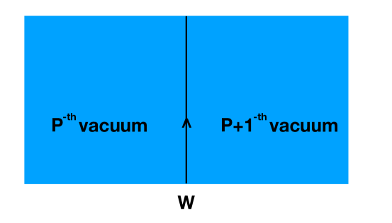
Figure 1: Two DW vacua (43) separated by a fundamental quark worldline (Euclidean). As explained in Section 3, $W$ can be viewed as the end of a confining string worldsheet extending into the ${\mathbb{R}}^{3}$ bulk. The picture holds in the high-$T$ DW on ${\mathbb{R}}^{3}\times S^{1}_{\beta}$, associated with center symmetry breaking. It also applies in the zero-$T$ ${\mathbb{R}}^{3}\times{\mathbb{S}}^{1}_{L}$, in the semiclassically calculable $\Lambda NL\ll 1$ regime, where the DW is associated with chiral symmetry breaking. In both the small-$\beta$ and small-$L$ case, the DW worldvolume is $2$-D. In the small-$L$ case, the $N$ $P$-vacua are represented by distinct semiclassical DW solutions ($N$ such solutions are known to exist for $k=1$), each carrying one-half the fundamental quark flux, see Anber:2015kea ; Anber:2015wha ; Poppitz:2017ivi ; Anber:2017tug for details. The resemblance between the small-$\beta$ and small-$L$ cases is because the relevant ’t Hooft anomalies on the DW are saturated in a similar mode. Note that on ${\mathbb{R}}^{3}\times{\mathbb{S}}^{1}_{L}$, confinement in the ${\mathbb{R}}^{3}$ bulk is abelian Unsal:2007jx , in contrast to the small-$\beta$ case.

We pause to note that essentially the same picture—different vacua on the DW worldvolume are separated by probe quarks—was found, by an explicit semiclassical analysis, to hold on DW between chirally broken vacua of super-YM in the calculable regime on ${\mathbb{R}}^{3}\times{\mathbb{S}}^{1}$. While a TQFT description was not given in Anber:2015kea , here we note that (45) can also be used there, with the $0$-form ${\mathbb{Z}}_{N}$ of the TQFT being the $0$-form center symmetry along the compact ${\mathbb{S}}^{1}$ (unbroken in the bulk, but broken on the DW). The $1$-form ${\mathbb{Z}}_{N}$ is the same bulk-${\mathbb{R}}^{3}$ center symmetry as in the present high-$T$ discussion, see Figure 1 for an illustration.

Continuing with the high-$T$ theory, in order to see that the topological “chiral lagrangian” (45) matches the mixed anomaly, consider gauging the $1$-form center symmetry via the $2$-form ${\mathbb{Z}}_{N}$ gauge field $B^{(2)}$ (reverting back to Euclidean space and rearranging factors of $N$ and $2\pi$ in (45) for convenience):

$$S_{2-D}=i\;{2\pi\over N}\int\limits_{M_{2}}{N\varphi^{(0)}\over 2\pi}\wedge{N(da^{(1)}-B^{(2)})\over 2\pi}~{},$$ (47)

consistent with the gauged $1$-form invariance $a^{(1)}\rightarrow a^{(1)}+\lambda^{(1)}$ and $B^{(2)}\rightarrow B^{(2)}+d\lambda^{(1)}$. As per our earlier discussion (see Footnote 15) the $1$-form transformation parameter has quantized flux $\oint d\lambda^{(1)}\in 2\pi{\mathbb{Z}}$ and $\oint B^{(2)}={2\pi{\mathbb{Z}}\over N}$. Under a chiral transformation $\delta\varphi^{(0)}={2\pi\over N}$, in the background of $p$ units of ’t Hooft flux, $\oint_{M_{2}}{NB^{(2)}\over 2\pi}=p$, we have

$$\delta_{{\mathbb{Z}}_{N}^{d\chi}}S_{2-D}=i\;{2\pi\over N}\int\limits_{M_{2}}{N(da^{(1)}-B^{(2)})\over 2\pi}~{}=-i\;{2\pi p\over N},$$ (48)

as required by the anomaly (34).

Assuming that the ${\mathbb{Z}}_{2N}^{d\chi}\rightarrow{\mathbb{Z}}_{2}$ breaking pattern (43) holds for all $k$-walls, the TQFT describing the IR $k$-wall physics should also be given by (45), as the $k>1$ theory has the same number of vacua. As noted in the paragraph after (34), turning on a unit ’t Hooft flux in the bulk theory corresponds to $k$ units of fractional $U(1)$ flux on the $k$-wall, i.e. $\oint_{M_{2}}{NB^{(2)}\over 2\pi}=k$, so the anomaly (34) is also matched.

5 $\mathbf{k}$-walls in QCD(adj)

Finally, we comment on the $k$-walls in $SU(N)$ QCD(adj), which is a Yang-Mills theory endowed with $n_{f}$ adjoint Weyl fermions. As in SYM, the UV Lagrangian of this theory is invariant under a global $U(1)_{R}$ axial symmetry. This symmetry, however, is anomalous and breaks down to the anomaly-free ${\mathbb{Z}^{d\chi}_{2Nn_{f}}}$ discrete chiral symmetry. In addition, the theory is invariant under a global $SU(n_{f})$ symmetry, such that the adjoint fermions transform in the fundamental representation of $SU(n_{f})$.

Everything we said about the wall action in SYM transcends naturally to QCD(adj); the only difference is an additional factor of $n_{f}$ multiplying $(-1)^{n}$ in (11), which amounts to scaling the wall tension by a trivial numerical coefficient. The worldvolume of the $k$-wall is also a $2$-D QCD with gauge group $U(1)\times SU(N-k)\times SU(k)$ and fermions charged under $U(1)$ and transforming in the bi-fundamental representation of $SU(N-k)\times SU(k)$. In addition, as in the UV theory, the fermions transform in the fundamental representation of the global $SU(n_{f})$. Under an axial $U(1)_{R}$ transformation $\psi_{\pm}\rightarrow e^{i\chi}\psi_{\pm}$ the measure transforms as in (19), with ${\cal J}$ now replaced by

$${\cal J}\equiv\exp\left[i\;2n_{f}\chi(N-k)k\;\gamma^{(N-k)}\oint{F_{12}^{N-k}dx^{1}dx^{2}\over 2\pi}\right]\,,$$ (49)

i.e., there is an extra factor of $n_{f}$ in the Jacobian. Repeating the same steps from (19) to (21), one can easily see that there is an anomaly-free $\mathbb{Z}^{d\chi}_{2n_{f}N}$ discrete chiral symmetry on the DW. Similarly, it is straightforward to see that there is a mixed discrete ’t Hooft anomaly upon turning on a $p$-twist of $SU(N)$: ${\cal J}=e^{-i{2\pi\over N}kp}$.

Yet, the most interesting part of the story is the fate of the discrete $\mathbb{Z}_{2n_{f}N}^{d\chi}$ and global $SU(n_{f})$ symmetries on the wall. Since our theory lives in $2$-D, one expects that $SU(n_{f})$ remains unbroken in the IR, as suggested by the Coleman theorem Coleman:1973ci . Interestingly, one can use the nonabelian bosonization and WZW model, discussed in Section 4, to show that this is indeed the case. Let us for simplicity consider the $k=1$-wall. Now, since there is an extra $SU(n_{f})$ global symmetry, the bosonization rule (42) should be replaced by

$$\bar{\psi}_{+}^{a\,i}\psi_{-b\,j}=\mu\,h^{a}_{b}\;g^{i}_{j}\;e^{-i\sqrt{\frac{4\pi}{n_{f}(N-1)}}\phi}\,,$$ (50)

where, as before, $h$ and $e^{-i\sqrt{\frac{4\pi}{n_{f}(N-1)}}\phi}$ are boson fields, $SU(N-1)$- and $U(1)$-group valued, respectively, while $g$ is a global-$SU(n_{f})$ group-valued boson-field matrix. There are well-known subtleties with the above multi-flavor bosonization rule, which, however, have been argued to be not important for studying the low-energy physics in the strong coupling limit $e\gg m\rightarrow 0$ ($e$ is the $2$-D gauge coupling and $m$ the fermion mass) Affleck:1985wa , Frishman:1992mr . This is also the limit considered here and, for our qualitative considerations, we shall assume that (50) holds. As before, the correlators $\langle e^{-i\sqrt{\frac{4\pi}{n_{f}(N-1)}}\phi(x)}e^{i\sqrt{\frac{4\pi}{n_{f}(N-1)}}\phi(y)}\rangle$ and $\left\langle\mbox{tr}h^{\dagger}(x)\;\mbox{tr}h(y)\right\rangle$ approach constants in the limit $|x-y|\rightarrow\infty$, thanks to the gauging of $U(1)\times SU(N-1)$. The correlator $\langle g_{i}^{j}(x)g_{k}^{l}(y)\rangle$, however, behaves as Knizhnik:1984nr

$$\left\langle g_{i}^{j}(x)g_{k}^{l}(y)\right\rangle=\frac{\delta_{i}^{l}\delta_{k}^{j}}{\left[M|x-y|\right]^{\frac{n_{f}^{2}-1}{n_{f}(n_{f}+N-1)}}}\,,$$ (51)

and $M$ is a mass scale. Next, we define the $SU(N-1)$ color-singlet operator

$${\cal O}^{(1)\,i}_{j}\equiv\bar{\psi}_{+}^{a\,i}\psi_{-a\,j}\,,$$ (52)

which transforms non-trivially under $SU(n_{f})$. Then, we can use (50) and (51) to show that $\langle{\cal O}^{(1)\,\dagger i}_{j}(x){\cal O}^{(1)\,i}_{j}(y)\rangle\rightarrow 0$ as $|x-y|\rightarrow\infty$. Therefore, we find

$$\langle\bar{\psi}_{+}^{a\,i}\psi_{-a\,j}\rangle=0\,,$$ (53)

and conclude that $SU(n_{f})$ is unbroken in the IR, in accord with the Coleman theorem.

What remains is to examine the discrete chiral symmetry $\mathbb{Z}_{2n_{f}N}^{d\chi}$. To this end we consider the color-singlet and $SU(n_{f})$-singlet operator

$${\cal O}^{(2)}(x)\equiv\det\limits_{i,j}\bar{\psi}_{+}^{a\,i}(x)\psi_{-a\,j}(x).$$ (54)

It is trivial to see that ${\cal O}^{(2)}$ acquires a phase $e^{i\frac{2\pi}{N}}$ under a $\mathbb{Z}_{2n_{f}N}^{d\chi}$ transformation, and hence, it can be used to examine the breaking of $\mathbb{Z}_{2n_{f}N}^{d\chi}$. As it is an $SU(n_{f})$ singlet, it is possible that the correlator (51) of the $SU(n_{f})$-valued bosonic field $g^{i}_{j}$, which disorders the fermion bilinear (52), does not similarly affect the ${\cal O}^{(2)}$ two-point correlation function. If so, $\langle{\cal O}^{(2)}(x){\cal O}^{(2)\;\dagger}(y)\rangle$ would approach constant at infinite $|x-y|$. Then, $\mathbb{Z}_{2n_{f}N}^{d\chi}$ is broken down to $\mathbb{Z}_{2n_{f}}^{d\chi}$ on the $k=1$-wall leading to $N$ distinct vacua on the wall, a result that also generalizes to the $k$-wall. In this scenario, the IR spectrum of the $k$-wall in QCD(adj) would be free from massless excitations, and the mixed anomaly would be matched by a TQFT describing the $N$ vacua, exactly as in SYM.

Acknowledgments:

We thank Zohar Komargodski for discussions. MA is supported by an NSF grant PHY-1720135. EP is supported by a Discovery Grant from NSERC.

Appendix A Group theory conventions

We denote the fundamental $SU(N)$ generators by $H^{a}$, $a=1,...,N-1$. An explicit form is $H^{a}={\rm diag}[\lambda^{a1},...,\lambda^{aN}]$, where

$$H^{a} = {\rm diag}[\lambda^{a1},...,\lambda^{aN}]={1\over\sqrt{a(a+1)}}{\rm diag}[\underbrace{1,1,...,1}_{a\,\mbox{\small times}},-a,\underbrace{0,0,...0}_{N-1-a\,\mbox{\small times}}]~{}$$ (55)

$$\lambda^{aA} \equiv {1\over\sqrt{a(a+1)}}(\theta^{aA}-a\delta_{a+1,A}),~{}a=1,...,N-1,~{}A=1,...,N,~{}\theta^{aA}\equiv\left\{\begin{array}[]{c}1,a\geq A\cr 0,a<A\end{array}\right.$$ (58)

The only utility in introducing $\lambda^{aA}$ in (55) is to note that the weights of the fundamental representation $\bm{\nu}^{A}$ can be expressed in this $N-1$-dimensional basis (we denote its $a$-th component by $(\bm{\nu}^{A})_{a}$) as:

$$(\bm{\nu}^{A})_{a}=\lambda^{aA},~{}~{}\bm{\nu}^{A}\cdot\bm{\nu}^{B}\equiv\sum\limits_{a=1}^{N-1}\lambda^{aA}\lambda^{aB}=\delta^{AB}-{1\over N},~{}\sum\limits_{A=1}^{N}\lambda^{aA}\lambda^{bA}=\delta^{ab}~{},$$ (59)

where we also noted the properties of the $\lambda^{aA}$ implying that $\mathrm{tr}\,H^{a}H^{b}=\delta^{ab}$.

Furthermore, the fundamental weights and simple roots of $SU(N)$ which we denote by $\bm{\omega}^{a}$ and $\bm{\alpha}^{a}$, respectively, are

$$\bm{\omega}^{a} = \sum\limits_{A=1}^{a}\bm{\nu}^{A},~{}a=1,\ldots N-1,$$ (60)

$$\bm{\alpha}^{a} = \bm{\nu}^{a}-\bm{\nu}^{a+1},~{}a=1,\ldots N-1.$$

We also define the positive roots $\bm{\beta}^{AB}$, $A<B$:

$$\bm{\beta}^{AB}\equiv\bm{\nu}^{A}-\bm{\nu}^{B}~{},~{}A,B=1,\ldots N.$$ (61)

The simple roots are a subset, $\bm{\alpha}^{a}=\bm{\beta}^{a\;a+1}$ and the affine root is $\bm{\alpha}^{0}=-\sum\limits_{k=1}^{N-1}\bm{\alpha}^{k}$. We shall need several relations that follow from the definitions (55, 59, 60):

$$\bm{\omega}^{a}\cdot\bm{\omega}^{b} = {\rm min}(a,b)-{ab\over N}$$ (62)

$$\bm{\omega}^{b}\cdot\bm{H} = \sum\limits_{a=1}^{N-1}(\bm{\omega}^{b})_{a}H^{a}={\rm diag}[\underbrace{1-{b\over N},1-{b\over N},...,1-{b\over N}}_{b\,\mbox{\small times}},\underbrace{-{b\over N},-{b\over N},...-{b\over N}}_{N-b\,\mbox{\small times}}]$$ (63)

$$\bm{\omega}^{b}\cdot\bm{\beta}^{AB} = \sum\limits_{k=1}^{b}\delta^{kA}-\delta^{kB}=\left\{\begin{array}[]{cc}0,&b<A\cr 1,&A\leq b<B\cr 0,&b\geq B\end{array}\right.~{}.$$ (67)

Next, as will be seen below, on the DW the $SU(N)$ group breaks to $U(1)\times SU(k)\times SU(N-k)$. Here we introduce some algebraic notation that will be useful to study the DW theory. We define the unbroken $U(1)$ generator as

$$\tilde{H}^{N-k}=\frac{1}{\sqrt{kN(N-k)}}\mbox{diag}\left[\underbrace{k,k,...,k}_{N-k\,\mbox{\small times}},\underbrace{k-N,k-N,...,k-N}_{k\,\mbox{\small times}}\right]\,,$$ (68)

satisfying $\mbox{tr}\left[\tilde{H}^{N-k}\tilde{H}^{N-k}\right]=1$ (we use the tilde to stress that this is not one of the $H^{a}$ previously introduced in (55), but can be expressed as their linear combination). Further, we break the Lie-algebra generators of $SU(N)$ as follows (omitting $\tilde{H}^{N-k}$ (68), which commutes with the $SU(N-k)$ and $SU(k)$ hermitean generators ${\cal T}^{a}$ and ${\cal T}^{A}$)

$$T=\left[\begin{array}[]{cc}{\cal T}^{a}_{(N-k)\times(N-k)}&E_{\bm{\beta}\,(N-k)\times k}\\ E_{-\bm{\beta}\,k\times(N-k)}&{\cal T}^{A}_{k\times k}\end{array}\right]\,,$$ (71)

where the subscript indicates the matrix dimensionality. There are $a=1,2,..,(N-k)^{2}-1$ $SU(N-k)$ generators ${\cal T}^{a}$, $A=1,2,...,k^{2}-1$ $SU(k)$ generators ${\cal T}^{A}$, and $2k(N-k)$ generators $E_{\pm\bm{\beta}}$ corresponding to $2k(N-k)$ different roots of $SU(N)$. This adds up to the original $N^{2}-1$ generators of $SU(N)$. We shall not need to explicitly define the ${\cal T}^{a}$ and ${\cal T}^{A}$ generators.

Explicitly, we define the $(N-k)\times k$ matrix $E_{\bm{\beta}\,}$ as follows. First, to enumerate the roots $\beta$, we denote them as $\beta_{AA^{\prime}}$, with $A=1,...,N-k$ and $A^{\prime}=1,...,K$. Next, regarding $E_{\bm{\beta}_{AA^{\prime}}}$ as an $(N-k)\times k$ matrix, we define its matrix elements as

$$(E_{\bm{\beta}_{AA^{\prime}}})_{BB^{\prime}}=\delta_{AB}\delta_{A^{\prime}B^{\prime}},~{}B=1,...,N-k,~{}~{}B^{\prime}=1,...,k.$$ (72)

Clearly, these are $k(N-k)$ linearly independent generators. The matrices $E_{-\bm{\beta}}$ are similarly defined: these are $k\times(N-k)$ matrices, labeled by $-\bm{\beta}_{AA^{\prime}}$, with matrix elements

$$(E_{-\bm{\beta}_{AA^{\prime}}})_{B^{\prime}B}=\delta_{AB}\delta_{A^{\prime}B^{\prime}},~{}B=1,...,N-k,~{}~{}B^{\prime}=1,...,k.$$ (73)

In matrix form, we have that $E_{-\bm{\beta}_{AA^{\prime}}}=(E_{\bm{\beta}_{AA^{\prime}}})^{T}$. The explicit form (72, 73) of $E_{\pm\bm{\beta}}$ implies the following relations that we shall use in the following:

$$\mathrm{tr}\,(E_{\bm{\beta}_{CC^{\prime}}}E_{-\bm{\beta}_{BB^{\prime}}}) = \delta_{CB}\delta_{C^{\prime}B^{\prime}}$$

$$\mathrm{tr}\,(E_{\bm{\beta}_{CC^{\prime}}}{\cal T}^{A}E_{-\bm{\beta}_{BB^{\prime}}}) = \delta_{CB}{\cal T}^{A}_{C^{\prime}B^{\prime}}$$ (74)

$$\mathrm{tr}\,(E_{-\bm{\beta}_{CC^{\prime}}}{\cal T}^{a}E_{\bm{\beta}_{BB^{\prime}}}) = \delta_{C^{\prime}B^{\prime}}{\cal T}^{a}_{CB}.$$

It is now straightforward to prove the relations that follow (the index convention below is the one from the previous paragraph: primed indices range from $1,...,k$ and unprimed from $1,...,N-k$):

$$\left[\tilde{H}^{N-k},E_{\pm\bm{\beta}_{AA^{\prime}}}\right] = \pm\gamma^{(N-k)}E_{\pm\bm{\beta}_{AA^{\prime}}}\,,~{}~{}\gamma^{(N-k)}\equiv\sqrt{\frac{N}{k(N-k)}},$$

$$(\left[{\cal T}^{a},E_{\bm{\beta}_{AA^{\prime}}}\right])_{BB^{\prime}} \equiv ({\cal T}^{a}E_{\bm{\beta}_{AA^{\prime}}})_{BB^{\prime}}=\sum_{C}({\cal T}^{a})_{BC}(E_{\bm{\gamma}_{AA^{\prime}}})_{CB^{\prime}}\,,$$

$$(\left[{\cal T}^{a},E_{-\bm{\beta}_{AA^{\prime}}}\right])_{B^{\prime}B} = -(E_{-\bm{\beta}_{AA^{\prime}}}{\cal T}^{a})_{B^{\prime}B}=-\sum_{C}(E_{-\bm{\beta}_{AA^{\prime}}})_{B^{\prime}C}({\cal T}^{a})_{CB}\,,$$ (75)

$$(\left[{\cal T}^{A},E_{\bm{\beta}_{AA^{\prime}}}\right])_{BB^{\prime}} = -(E_{\bm{\beta}_{AA^{\prime}}}{\cal T}^{A})_{BB^{\prime}}=-\sum_{C^{\prime}}(E_{\bm{\beta}_{AA^{\prime}}})_{BC^{\prime}}({\cal T}^{A})_{C^{\prime}B^{\prime}}\,,\quad$$

$$(\left[{\cal T}^{A},E_{-\bm{\beta}}\right])_{B^{\prime}B} = ({\cal T}^{A}E_{-\bm{\beta}})_{B^{\prime}B}=\sum_{C^{\prime}}({\cal T}^{A})_{B^{\prime}C^{\prime}}(E_{-\bm{\beta}_{AA^{\prime}}})_{C^{\prime}B}\,.$$

We kept the top equation in (A) in matrix form, where we extended the $(N-k)\times k$ matrix $E_{\bm{\beta}}$ to an $N\times N$ matrix by embedding as in (71). The rest of the equations representing the action of the $SU(N-k)$ and $SU(k)$ generators was shown explicitly using index notation, consistent with the definitions (72, 73, 71).

Appendix B Fermion zero modes

To find the fermion zero modes, we begin with the covariant derivative containing the $\lambda^{\beta}$ fermions, as explained in Section 2.3 of the main text. Using the decompositions (16), and recalling the action of ${\cal T}^{a,A}$ on $E_{\pm\beta}$ of (A) which we use below in matrix form (a summation over $C$ is from $1,...,N-k$ and $C^{\prime}$ from $1,...,k$ is understood below), it is given by

$$\partial_{\mu}\lambda-i[A_{\mu},\lambda] = ~{}~{}\partial_{\mu}\lambda^{\bm{\beta}_{CC^{\prime}}}E_{\bm{\beta}_{CC^{\prime}}}+\partial_{\mu}\lambda^{-\bm{\beta}_{CC^{\prime}}}E_{-\bm{\beta}_{CC^{\prime}}}$$ (76)

$$-i\gamma^{(N-k)}A_{\mu}^{N-k}(\lambda^{\bm{\beta}_{CC^{\prime}}}E_{\bm{\beta}_{CC^{\prime}}}-\lambda^{-\bm{\beta}_{CC^{\prime}}}E_{-\bm{\beta}_{CC^{\prime}}})$$

$$-iA^{a}_{\mu}\;({\cal T}^{a}E_{\bm{\beta}_{CC^{\prime}}}\lambda^{\bm{\beta}_{CC^{\prime}}}-E_{-\bm{\beta}_{CC^{\prime}}}{\cal T}^{a}\lambda^{-\bm{\beta}_{CC^{\prime}}})$$

$$+iA^{A}_{\mu}\;(E_{\bm{\beta}_{CC^{\prime}}}{\cal T}^{A}\lambda^{\bm{\beta}_{CC^{\prime}}}-{\cal T}^{A}E_{-\bm{\beta}_{CC^{\prime}}}\lambda^{-\bm{\beta}_{CC^{\prime}}})~{}$$

Because the matrices $E_{\bm{\beta}}$, ${\cal T}^{a}E_{\bm{\beta}}$, $E_{\bm{\beta}}{\cal T}^{A}$ and the matrices $E_{-\bm{\beta}}$, ${\cal T}^{A}E_{-\bm{\beta}}$, $E_{-\bm{\beta}}{\cal T}^{a}$ are in orthogonal subspaces of $SU(N)$, we can write the equations of motion for $\lambda^{\bm{\beta}}$ and $\lambda^{-\bm{\beta}}$ separately as follows:

$$\bar{\sigma}^{\mu} ( \partial_{\mu}\lambda^{\bm{\beta}_{CC^{\prime}}}E_{\bm{\beta}_{CC^{\prime}}}-i\gamma^{(N-k)}A_{\mu}^{N-k}\lambda^{\bm{\beta}_{CC^{\prime}}}E_{\bm{\beta}_{CC^{\prime}}}$$

$$-iA^{a}_{\mu}\;{\cal T}^{a}E_{\bm{\beta}_{CC^{\prime}}}\lambda^{\bm{\beta}_{CC^{\prime}}}+iA^{A}_{\mu}\;E_{\bm{\beta}_{CC^{\prime}}}{\cal T}^{A}\lambda^{\bm{\beta}_{CC^{\prime}}})=0~{},$$

$$\bar{\sigma}^{\mu} ( \partial_{\mu}\lambda^{-\bm{\beta}_{CC^{\prime}}}E_{-\bm{\beta}_{CC^{\prime}}}+i\gamma^{(N-k)}A_{\mu}^{N-k}\lambda^{-\bm{\beta}_{CC^{\prime}}}E_{-\bm{\beta}_{CC^{\prime}}}$$ (77)

$$+iA^{a}_{\mu}\;E_{-\bm{\beta}_{CC^{\prime}}}{\cal T}^{a}\lambda^{-\bm{\beta}_{CC^{\prime}}}-iA^{A}_{\mu}\;{\cal T}^{A}E_{-\bm{\beta}_{CC^{\prime}}}\lambda^{-\bm{\beta}_{CC^{\prime}}})=0~{}.$$

We now multiply the first equation in (B) by $E_{-\bm{\beta}_{BB^{\prime}}}$ and take the trace to obtain the equation for $\lambda^{\bm{\beta}_{BB^{\prime}}}$:

$$0 = \bar{\sigma}^{\mu}\left(\partial_{\mu}\lambda^{\bm{\beta}_{BB^{\prime}}}-iA^{N-k}_{\mu}\gamma^{(N-k)}\lambda^{\bm{\beta}_{BB^{\prime}}}-iA_{\mu}^{a}{\cal T}^{a}_{BD}\lambda^{\bm{\beta}_{DB^{\prime}}}+iA_{\mu}^{A}\lambda^{\bm{\beta}_{BD^{\prime}}}{\cal T}^{A}_{D^{\prime}B^{\prime}}\right).$$ (78)

Eqn. (78) shows that $\lambda^{\bm{\beta}_{BB^{\prime}}}$, considered as the $BB^{\prime}$-th element of a $(N-k)\times k$ matrix $\lambda^{\bm{\beta}}$, transforms as $\lambda^{\bm{\beta}}\rightarrow U_{N-k}\;\lambda^{\bm{\beta}}\;U^{\dagger}_{k}$ under $SU(N-k)\times SU(k)$ gauge transformations, where $U_{N-k}=e^{i\omega^{a}{\cal T}^{a}}$, $U_{k}=e^{i\omega^{A}{\cal T}^{A}}$. It is easy to see that the (78) is invariant under these transformation, along with $A_{\mu}^{a}{\cal T}^{a}\rightarrow U_{N-k}(A_{\mu}^{a}{\cal T}^{a}+i\partial_{\mu})U_{N-k}^{\dagger}$ and $A_{\mu}^{A}{\cal T}^{A}\rightarrow U_{k}(A_{\mu}^{A}{\cal T}^{A}+i\partial_{\mu})U_{k}^{\dagger}$.

Next, proceeding as in the derivation of (B), multiplying the second equation by $E_{\bm{\beta}_{BB^{\prime}}}$ and taking the trace, we obtain the equation of motion for $\lambda^{-\bm{\beta}_{BB^{\prime}}}$:

$$0 = \bar{\sigma}^{\mu}\left(\partial_{\mu}\lambda^{-\bm{\beta}_{BB^{\prime}}}+iA^{N-k}_{\mu}\gamma^{(N-k)}\lambda^{-\bm{\beta}_{BB^{\prime}}}+i\lambda^{-\bm{\beta}_{DB^{\prime}}}{\cal T}^{a}_{DB}A_{\mu}^{a}-iA_{\mu}^{A}{\cal T}^{A}_{B^{\prime}D^{\prime}}\lambda^{-\bm{\beta}_{BD^{\prime}}}\right)$$ (79)

Considering $\lambda^{-\bm{\beta}_{BB^{\prime}}}$ as the $B^{\prime}B$-th entry of a $k\times(N-k)$ matrix $\lambda^{-\bm{\beta}}$, we conclude that it transforms as $\lambda^{-\bm{\beta}}\rightarrow U_{k}\;\lambda^{-\bm{\beta}}U_{N-k}^{\dagger}$ under $SU(N-k)\times SU(k)$ gauge transformations.

Finally, the transformation of $\lambda^{\bm{\beta}}$, $\lambda^{-\bm{\beta}}$ under the $U(1)$ as $\lambda^{\pm\beta}\rightarrow e^{\pm i\omega\gamma^{(N-k)}}\lambda^{\pm\beta}$, with $A_{\mu}^{N-k}\rightarrow e^{i\omega}(A_{\mu}^{N-k}+i\partial_{\mu})e^{-i\omega}$; these are inherited from the $SU(N)$ transformation $e^{i\omega\tilde{H}^{N-k}}$. The transformation properties of the fermions under the unbroken gauge group on the $k$-wall are summarized in Table 2.

To find the fermion zero modes in the $k$-wall background, we now restrict the gauge backgrounds in the equations of motion (78,79) to the $k$-wall background (7). We also decompose the fermions into Matsubara modes, $\lambda^{\pm\beta}_{p}$, defined as $\lambda^{\pm\beta}(x^{4},x^{i})=\sum_{p\in{\mathbb{Z}}}\lambda_{p}^{\pm\beta}(x^{i})e^{i2\pi Tp^{\prime}x^{4}}$, where $p^{\prime}\equiv p+1/2$. In the $k$-wall background, the equations of motion for the different Matsubara modes decouple.

The $k$-wall is orthogonal to the $z=x^{3}$ direction, with worldvolume along $x^{1,2}$ and, recalling that $\bar{\sigma}^{\mu}=(\bm{\sigma},-i\sigma^{0})$, we obtain the $z$-dependent Weyl equation

$$0=\left[\sigma^{3}\partial_{z}+\sigma^{0}\left(2\pi p^{\prime}T\mp TQ^{(k)}(z)\gamma^{(N-k)}\right)\right]\lambda^{\pm\bm{\beta}}_{p}~{},$$ (80)

where the signs are correlated. The solution of this equation is

$$\lambda_{p}^{\pm\bm{\beta}}(z)=e^{~{}\sigma^{3}\left[-2\pi p^{\prime}Tz\pm T\gamma^{(N-k)}\int\limits_{0}^{z}Q^{(k)}(z^{\prime})dz^{\prime}\right]}\;\lambda_{p}^{\pm\bm{\beta}}(0).$$ (81)

We now recall from (9) that $Q^{(k)}(z)$ vanishes as $z\rightarrow-\infty$ and $\int\limits^{z\rightarrow-\infty}_{0}Q^{(k)}(z^{\prime})dz^{\prime}$ converges. Thus normalizability of the solutions as $z\rightarrow-\infty$ is only determined by the first term in the exponent of (81), requiring that only wave functions $\lambda_{p}^{\pm\bm{\beta}}(0)$ which are eigenstates of $\sigma^{3}$ with $\sigma^{3}p^{\prime}<0$ lead to a zero mode normalizable as $z\rightarrow-\infty$. On the other hand, as $z\rightarrow\infty$, the boundary conditions imply that $\gamma^{(N-k)}\int\limits^{z\rightarrow+\infty}_{0}Q^{(k)}(z^{\prime})dz^{\prime}\rightarrow-2\pi z$. Thus normalizability of (81) at $z\rightarrow+\infty$ requires that $\lambda_{p}^{\pm\bm{\beta}}(0)$ also be eigenvalues of $\sigma^{3}$ with $-\sigma^{3}p^{\prime}\mp\sigma^{3}<0$.

To proceed, we recall that $\lambda^{\pm\beta}_{p}$ are two-component Weyl spinors. We denote their upper components $\lambda^{\pm\beta}_{p,1}$ (with $+1$ eigenvalue of $\sigma^{3})$ and the lower components by $\lambda^{\pm\beta}_{p,2}$ (with $-1$ eigenvalue of $\sigma^{3})$. We further note that the upper $\lambda^{\pm\beta}_{p,1}$ (lower $\lambda^{\pm\beta}_{p,2}$) components obey a positive (negative) two-dimensional chirality Weyl equation, as follows from our definition of $\bar{\sigma}^{\mu}$. The two conditions for normalizability stated after (81) admit (recalling $p^{\prime}=p+1/2$) only the following solutions:

$$\lambda^{\bm{\beta}}_{p=-1,1}: \psi_{+},\;\;{\rm left\;mover},(\gamma^{(N-k)},\Box,\overline{\Box})\;{\rm under}\;(U(1),SU(N-k),SU(k)),$$

$$\lambda^{-\bm{\beta}}_{p=0,2}: \psi_{-},\;\;{\rm right\;mover},(-\gamma^{(N-k)},\overline{\Box},\Box)\;{\rm under}\;(U(1),SU(N-k),SU(k)),$$ (82)

where we also display their quantum numbers under the unbroken gauge group on the $k$-wall. The information contained in (B) is also shown in Table 2. There, we also note that the zero modes have the same charge under the anomalous chiral symmetry of the bulk $4$-D theory as they originate in the same $4$-D Weyl fermion. Finally, as in the case of the $SU(2)$ theory of ref. Anber:2018jdf , the $2$-D $k$-wall worldvolume theory is an axial one: the $R-$ and $L$-moving fermions have opposite charges under all gauge groups; nonetheless, it is clear that the $2$-D $U(1)\times SU(N-k)\times SU(k)$ gauge theory with matter content given in (B) is gauge anomaly free. For brevity, we rename the two $2$-D Weyl fermions $\psi_{+}$ and $\psi_{-}$ as shown also in Table 2.

	$\lambda^{\bm{\beta}}$	$\lambda^{-\bm{\beta}}$
gauge $U(1)$	$\gamma^{(N-k)}=\sqrt{\frac{N}{k(N-k)}}$	$-\gamma^{(N-k)}=-\sqrt{\frac{N}{k(N-k)}}$
gauge $SU(k)$	$\overline{\Box}$	$\Box$
gauge $SU(N-k)$	$\Box$	$\overline{\Box}$
$2$-D chirality	left mover	right mover
global $U(1)_{R}$	1	1
$2$-D field	$\psi_{+}$	$\psi_{-}$

Table 2: Charges of the fermions $\lambda^{\beta}$ (see (16)) under the unbroken gauge group on the $k$-wall. In the bottom two rows, we show the normalizable zero modes’ $2$-D chirality and their charge under the anomalous $4$-D $U(1)_{R}$ chiral symmetry. The bottom line in the table introduces the $2$-D notation for the Weyl fermions of the $k$-wall theory, see also eq. (B).

Appendix C $\mathbf{U(1)}$ flux quantization

In order to understand $U(1)$ charge quantization, we need to recall the description of boundary conditions on the torus as in tHooft:1979rtg ; vanBaal:1982ag . We begin by recalling the description of gauge bundles in the $U(1)\times SU(N-k)\times SU(k)$ theory on the two-torus ($0\leq x_{1}\leq L_{1}$, $0\leq x_{2}\leq L_{2}$). These are described by transition functions $\Omega_{i\;[1]},\Omega_{i\;[N-k]},\Omega_{i\;[k]}$, where $[1],[N-k],[k]$ indicates the gauge group and $i=1,2$ the direction on the torus. The gauge fields obey the boundary conditions:

$$A_{\;[b]}(L_{1},x_{2}) = \Omega_{1\;[b]}(x_{2})\left(A_{\;[b]}(0,x_{2})+id\right)\Omega^{\dagger}_{1\;[b]}(x_{2})~{},$$

$$A_{\;[b]}(x_{1},L_{2}) = \Omega_{2\;[b]}(x_{1})\left(A_{\;[b]}(x_{1},0)+id\right)\Omega^{\dagger}_{2\;[b]}(x_{1})~{},$$ (83)

where  $[b]=[1],[N-k],[k]$. The transition functions $\Omega_{i\;[b]}$ are gauge group elements (the $U(1)$ boundary conditions are also given in (C) below). For $SU(N-k)$ and $SU(k)$, they are group elements in the defining representation. For later use, we embed them in $SU(N)$ as in (71):

$$\hat{\Omega}_{i\,[N-k]}=\left[\begin{array}[]{cc}\Omega_{i\,[N-k]}&0\\ 0&I_{k}\end{array}\right]~{},$$ (86)

where we indicated by $\hat{\Omega}$ that the transition function is embedded into $SU(N)$ and $I_{k}$ is a $k\times k$ unit matrix (in the following, we shall often omit the hat and the context will show whether the above embedding is used). Similarly, for $SU(k)$, we have

$$\hat{\Omega}_{i\,[k]}=\left[\begin{array}[]{cc}I_{N-k}&0\\ 0&\Omega_{i\,[k]}\end{array}\right]~{},$$ (89)

while the transition functions for $U(1)$ follow from the form of its generator, eqn. (68)

$$\Omega_{i\,[1]}=\left[\begin{array}[]{cc}e^{i2\pi\omega_{i}\frac{k}{N}\gamma^{(N-k)}}I_{N-k}&0\\ 0&e^{i2\pi\omega_{i}\frac{k-N}{N}\gamma^{(N-k)}}I_{k}\end{array}\right]~{}.$$ (92)

Further, from (C) it follows that under gauge transformations $g_{[b]}(x_{1},x_{2})$ ($0\leq x_{1}\leq L_{1}$, $0\leq x_{2}\leq L_{2}$) the transition functions transform

$$A_{\;[b]} \rightarrow g_{[b]}(A_{\;[b]}+id)g_{[b]}^{\dagger}$$

$$\Omega_{1\;[b]}(x_{2}) \rightarrow g_{[b]}(L_{1},x_{2})\;\Omega_{1\;[b]}(x_{2})\;g^{\dagger}_{[b]}(0,x_{2})~{},$$ (93)

$$\Omega_{2\;[b]}(x_{1}) \rightarrow g_{[b]}(x_{1},L_{2})\;\Omega_{2\;[b]}(x_{1})\;g^{\dagger}_{[b]}(x_{1},0)~{}.$$

The above gauge transformations and boundary conditions imply also that a fundamental Wilson loop winding the $i$-th direction of the torus requires an insertion of a transition function in order to be gauge invariant. For example, for $i=1$,

$$W_{[b]}(x_{2})=\mathrm{tr}\,(e^{i\int\limits_{0}^{L_{1}}A_{1\;[b]}(x_{1},x_{2})dx^{1}}\Omega_{1\;[b]}(x_{2}))~{}.$$ (94)

The transition functions must further obey the consistency conditions known as cocycle conditions, following from requiring that $A_{\;[b]}(L_{1},L_{2})$ be well defined (i.e. obtained from $A_{\;[b]}(0,0)$ along the two paths reaching $(L_{1},L_{2})$ from $(0,0)$). We begin with the cocycle conditions for the transition functions for $SU(N-k)$ and $SU(k)$

$$\Omega_{1\;[N-k]}(L_{2})\;\Omega_{2\;[N-k]}(0) = \left[\begin{array}[]{cc}e^{i{2\pi\over N-k}p_{N-k}}I_{N-k}&0\cr 0&I_{k}\end{array}\right]\;\Omega_{2\;[N-k]}(L_{1})\;\Omega_{1\;[N-k]}(0)$$ (97)

$$\Omega_{1\;[k]}(L_{2})\;\Omega_{2\;[k]}(0) = \left[\begin{array}[]{cc}I_{N-k}&0\cr 0&e^{i{2\pi\over k}p_{k}}I_{k}\end{array}\right]\;\Omega_{2\;[k]}(L_{1})\;\Omega_{1\;[k]}(0)~{}.$$ (100)

In $SU(N-k)$ and $SU(k)$ gauge theories, taken in isolation, the center elements appearing on the r.h.s. of (97, 100) equal unity, i.e. $p_{N-k}=p_{k}=0$.

We also recall that in $SU(N)$ gauge theories, there is a global one-form ${\mathbb{Z}}_{N}^{(1)}$ center symmetry acting on the transition functions. The boundary conditions for all fields are invariant under this symmetry if there are no fields in the fundamental representation (the boundary conditions for fundamental fields explicitly break the symmetry). The same holds for $SU(N-k)$ or $SU(k)$ gauge theories with only adjoint fields. For example, for $SU(N-k)$ there is a 1-form ${\mathbb{Z}}_{N-k}^{(1)}$ acting on the $SU(N-k)$ transition functions as

$$\Omega_{i\;[N-k]} \rightarrow z_{i\;[N-k]}\;\Omega_{i\;[N-k]}~{},~{}i=1,2,$$ (101)

where $z_{i\;[N-k]}\in{\mathbb{Z}}_{N-k}$ is an $x$-independent constant. The cocycle conditions (97) and all boundary conditions (in a theory without fundamental fields) are invariant under (101). The fundamental representation Wilson line operator (94) is the only one transforming under (101). This follows from the explicit appearance of the transition function in its gauge invariant definition, implying $W_{[N-k]}(x_{2})\rightarrow z_{1\;[N-k]}W_{[N-k]}(x_{2})$; similarly, a loop winding in the $x^{2}$ direction transforms by $z_{2\;[N-k]}$. We shall return to the one-form symmetries below when we consider the boundary conditions for the fermions in the $k$-wall theory.

We next write the $U(1)$ cocycle condition using the group element $e^{i\omega_{i}}$ as the $i$-th $U(1)$ transition function. Notice that (C), written for the $U(1)$ field $A^{N-k}$ as defined in (16) is simply

$$A^{N-k}(L_{1},x_{2}) = e^{i\omega_{1}(x_{2})}\left(A^{N-k}(0,x_{2})+id\right)e^{-i\omega_{1}(x_{2})}~{},$$

$$A^{N-k}(x_{1},L_{2}) = e^{i\omega_{2}(x_{1})}\left(A^{N-k}(x_{1},0)+id\right)e^{-i\omega_{2}(x_{1})}~{},$$ (102)

$$e^{i\omega_{1}(L_{2})}\;e^{i\omega_{2}(0)} = e^{i2\pi\alpha}\;e^{i\omega_{2}(L_{1})}\;e^{i\omega_{1}(0)}$$

while on the last line we wrote the $U(1)$ cocycle condition on the torus determined by a for now arbitrary phase. In terms of the $SU(N)$-embedded representation (92), the above $U(1)$ cocycle condition becomes

$$\Omega_{1\;[1]}(L_{2})\;\Omega_{2\;[1]}(0)=\left[\begin{array}[]{cc}e^{i2\pi\alpha\frac{k}{N}\gamma^{(N-k)}}I_{N-k}&0\\ 0&e^{i2\pi\alpha\frac{k-N}{N}\gamma^{(N-k)}}I_{k}\end{array}\right]\Omega_{2\;[1]}(L_{1})\;\Omega_{1\;[1]}(0)~{}.$$ (105)

The main point we want to stress now is that when the $U(1)\times SU(N-k)\times SU(k)$ theory arises from the adjoint-Higgs mechanism from the $SU(N)$ theory, the individual twists (nontrivial phases in the cocycle conditions) in (97, 100, 105) do not have to vanish, but can instead conspire to lead to zero twist in $SU(N)$. In other words, we consider the transition functions embedded in the $SU(N)$ theory and impose the cocycle condition for vanishing $SU(N)$ twist

$$e^{i{2\pi\over N}p_{N}}I_{N} = \left[\begin{array}[]{cc}e^{i\alpha\frac{2\pi k}{N}\gamma^{(N-k)}}I_{N-k}&0\\ 0&e^{i\alpha\frac{2\pi(k-N)}{N}\gamma^{(N-k)}}I_{k}\end{array}\right]\left[\begin{array}[]{cc}e^{i\frac{2\pi}{N-k}p_{N-k}}I_{N-k}&0\\ 0&I_{k}\end{array}\right]\left[\begin{array}[]{cc}I_{N-k}&0\\ 0&e^{i\frac{2\pi}{k}p_{k}}I_{k}\end{array}\right]$$ (112)

$$= \left[\begin{array}[]{cc}e^{i\alpha\frac{2\pi k}{N}\gamma^{(N-k)}}e^{i\frac{2\pi}{N-k}p_{N-k}}I_{N-k}&0\\ 0&e^{i\alpha\frac{2\pi(k-N)}{N}\gamma^{(N-k)}}e^{i\frac{2\pi}{k}p_{k}}I_{k}\end{array}\right]\,.$$ (115)

Above, we allowed for nonvanishing $SU(N)$ twist, $p_{N}\neq 0$ for future use; imposing vanishing $SU(N)$ twist corresponds to taking $p_{N}=0$. The above cocycle conditions, keeping $p_{N}\neq 0$, have the following general solution for $\alpha$, given below in one of many possible forms

$$\alpha\;\gamma^{(N-k)}\;k(N-k) = p_{N}(N-k)-Np_{N-k}-N(N-k)m_{4}$$ (116)

$$p_{k} = p_{N}-p_{N-k}-km_{5}-(N-k)m_{4}~{}~{}({\rm mod}\;N)$$ (117)

where $m_{4}$ and $m_{5}$ are arbitrary integers. On the top line we chose to express the $U(1)$ twist $\alpha$ in terms of the $SU(N)$ twist $p_{N}$ and the $SU(N-k)$ twist $p_{N-k}$. Note that the $SU(k)$ flux is determined by $p_{N},p_{N-k}$ and by the integers $m_{4}$ and $m_{5}$.

For further use, we also write the solution (116) in an equivalent way:

$$\alpha\gamma^{(N-k)}k(N-k) = (N-k)p_{k}-kp_{N-k}-m_{4}+m_{5}$$ (118)

$$p_{k}+p_{N-k} = p_{N}-km_{5}-(N-k)m_{4}~{}~{}({\rm mod}\;N)$$ (119)

The form (116) above is convenient to address our first task: what $U(1)$ fluxes are possible in the $SU(N)$ theory, i.e. for $p_{N}=0$ and varying $p_{N-k}$? The relation between $\alpha$ and $U(1)$ flux follows from using (C) to express the $U(1)$ flux through the torus in terms of the transition functions

$$\oint{F_{12}^{N-k}dx^{1}dx^{2}\over 2\pi}={1\over 2\pi}[\omega_{1}(L_{2})-\omega_{1}(0)-\omega_{2}(L_{1})+\omega_{2}(0)]=\alpha~{}.$$ (120)

where we used the $U(1)$ cocycle condition in the form (C). The above equation gives the $U(1)$ flux quantization condition: explicitly, we have, putting $p_{N}=0$ in (116):

$$\alpha=-\gamma^{(N-k)}(p_{N-k}+(N-k)m_{4})~{},$$ (121)

i.e. completely equivalent to eqn. (20) from the main text, which was used to conclude that the $k$-wall theory has a ${\mathbb{Z}}_{2N}$ anomaly free global symmetry inherited from the bulk theory. Another derivation of flux quantization, using constant flux backgrounds, is given in the main text, Section 2.4.1.

Before continuing our discussion of ’t Hooft flux backgrounds, we recall that the $2$-D fermions $\psi_{\pm}$ also satisfy a consistency condition on the corners of the torus (single valuedness of $\psi_{\pm}(L_{1},L_{2})$) given by

$$\psi_{\pm}(L_{1},L_{2})=\Omega_{1}(L_{2})\;\Omega_{2}(0)\circ\psi_{\pm}(0,0)=\Omega_{2}(L_{1})\;\Omega_{1}(0)\circ\psi_{\pm}(0,0),$$ (122)

where $\circ$ denotes the action of the $U(1)\times SU(N-k)\times SU(k)$ gauge transformations on the fermions and $\Omega$ collectively denotes the transition functions for the three gauge groups. Recalling the discussion after (78,79) of the gauge transformation properties of the fermions, we have explicitly $\Omega\circ\psi_{+}$ $=$ $e^{i\omega\gamma^{(N-k)}}\;\Omega_{[N-k]}\;\psi_{+}\;\Omega_{[k]}^{\dagger}$, $\Omega\circ\psi_{-}$ $=$ ${\epsilon}^{-i\omega\gamma^{(N-k)}}\;\Omega_{[k]}\;\psi_{+}\;\Omega_{[N-k]}^{\dagger}$. Thus the cocycle condition for $\psi_{+}$ (the $\psi_{-}$ condition does not bring new constraints) becomes

$$\psi_{+}(L_{1},L_{2})$$ (123)

$$= e^{i\omega_{1}(L_{2})\gamma^{(N-k)}}\;e^{i\omega_{2}(0)\gamma^{(N-k)}}\;\Omega_{1\;[N-k]}(L_{2})\;\Omega_{2\;[N-k]}(0)\;\psi_{+}(0,0)\;\Omega_{2\;[k]}^{\dagger}(0)\;\Omega_{1\;[k]}^{\dagger}(L_{2})$$

$$= e^{i\omega_{2}(L_{1})\gamma^{(N-k)}}\;e^{i\omega_{1}(0)\gamma^{(N-k)}}\;\Omega_{2\;[N-k]}(L_{1})\;\Omega_{1\;[N-k]}(0)\;\psi_{+}(0,0)\;\Omega_{1\;[k]}^{\dagger}(0)\;\Omega_{2\;[k]}^{\dagger}(L_{1})~{}.$$

The bulk $SU(N)$ theory has a ${\mathbb{Z}}_{N}^{(1)}$ 1-form global symmetry. The part of this 1-form symmetry projected to the $2$-D $k$-wall worldvolume is unbroken by the adjoint Higgsing and should still be manifest as a symmetry acting on transition functions, as described earlier. The transition functions $\Omega_{i\;[1]},\Omega_{i\;[N-k]},\Omega_{i\;[k]}$, collectively denoted by $\Omega_{i}$, embedded into $SU(N)$ are:

$$\Omega_{i}=\left[\begin{array}[]{cc}e^{i2\pi\omega_{i}\frac{k}{N}\gamma^{(N-k)}}\Omega_{i\;[N-k]}&0\\ 0&e^{i2\pi\omega_{i}\frac{k-N}{N}\gamma^{(N-k)}}\Omega_{i\;[k]}\end{array}\right]~{},~{}i=1,2.$$ (126)

Consider now the 1-form symmetry action (say, in the $x^{i}$ direction) on the transition functions:

$$e^{i\omega_{i}} \rightarrow e^{i2\pi\zeta_{(i)}}\;e^{i\omega_{i}},$$

$$\Omega_{i\;[N-k]} \rightarrow e^{i{2\pi\over N-k}q_{(i)N-k}}\;\Omega_{i\;[N-k]},$$ (127)

$$\Omega_{i\;[k]} \rightarrow e^{i{2\pi\over k}q_{(i)k}}\;\Omega_{i\;[k]}~{}.$$

In order that (126) transform by a ${\mathbb{Z}}_{N}$ phase $z_{i[N]}\equiv e^{i{2\pi\over N}p_{(i)}}$, i.e., $\Omega_{i}\rightarrow e^{i{2\pi\over N}p_{(i)}}\Omega_{i}$ as appropriate to a 1-form ${\mathbb{Z}}_{N}$ symmetry, the following conditions should hold

$$e^{i2\pi\zeta_{(i)}{k\over N}\gamma^{(N-k)}}\;e^{i{2\pi\over N-k}q_{(i)N-k}} = e^{i{2\pi\over N}~{}p_{(i)}}$$ (128)

$$e^{i2\pi\zeta_{(i)}{k-N\over N}\gamma^{(N-k)}}\;e^{i{2\pi\over k}q_{(i)k}} = e^{i{2\pi\over N}~{}p_{(i)}}$$

These conditions are formally equivalent to the ones in (112) determining the cocycle conditions for the $U(1)$ field (we stress that here they have a different meaning), upon the replacement $\alpha\rightarrow\zeta_{(i)}$, $p_{N-k}\rightarrow q_{(i)\;N-k}$, $p_{k}\rightarrow q_{(i)\;k}$, $p_{N}\rightarrow p_{(i)}$, and we can borrow their solutions. We express the solution (118, 119) for $\zeta_{(i)}$ as follows (setting $m_{4}$ and $m_{5}$ to zero)

$$\zeta_{(i)}\gamma^{(N-k)} = {q_{(i)k}\over k}-{q_{(i)N-k}\over N-k}$$ (129)

$$q_{(i)k}+q_{(i)N-k} = p_{(i)}~{}~{}({\rm mod}\;N)~{}.$$

These conditions ensure that (128) represent the action of a ${\mathbb{Z}}_{N}$ symmetry. It is easy to see that the $k$-wall fermion boundary conditions (123), are invariant under the ${\mathbb{Z}}_{N}^{(1)}$ symmetry action (128, 129). To further check (128, 129), consider the action on a fundamental $SU(N)$ Wilson loop. A fundamental of $SU(N)$ decomposes into two representations under the unbroken $U(1)\times SU(N-k)\times SU(k)$ gauge group: $q_{1}\sim(,{k\over N}\gamma^{(N-k)},\Box,{\bf 1})$ and $q_{2}\sim(({k-N\over N})\gamma^{(N-k)},{\bf 1},\Box)$, as seen from (68, 71). A Wilson loop of, say $q_{1}$, along the $x^{1}$ direction of the $k$-wall wordlvolume has the form

$$W_{q_{1}}(x_{2})=\mathrm{tr}\,(e^{i\int\limits_{0}^{L_{1}}A_{1\;[N-k]}(x_{1},x_{2})dx^{1}}\Omega_{1\;[N-k]}(x_{2}))\;e^{i{k\over N}\gamma^{(N-k)}\int\limits_{0}^{L_{1}}A_{1}^{N-k}(x_{1},x_{2})dx^{1}}e^{i\omega_{1}(x_{2}){k\over N}\gamma^{(N-k)}}$$ (130)

where we recalled (94) and inserted appropriate $SU(N-k)$ and $U(1)$ transition functions $\Omega_{1\;[N-k]},e^{i\omega_{1}{k\over N}\gamma^{(N-k)}}$. Under (C) with $i=1$, we have $W_{q_{1}}(x_{2})$ $\rightarrow$ $e^{i2\pi\zeta_{(1)}{k\over N}\gamma^{(N-k)}}$ $e^{i{2\pi\over N-k}q_{(1)N-k}}W_{q_{1}}(x_{2})$ $=$ $e^{i{2\pi\over N}p_{(1)}}W_{q_{1}}(x_{2})$, using (128, 129), as appropriate for a ${\mathbb{Z}}_{N}^{(1)}$ 1-form symmetry.

Appendix D ’t Hooft fluxes and projection of constant flux backgrounds

The discussion that follows is an explicit demonstration that the constant flux backgrounds (23) with $\bm{u}=\bm{\omega}^{b}$ are examples of backgrounds obeying the twisted boundary conditions (112) with nonzero $SU(N)$ twists, $p_{N}\neq 0$.

We begin with (25), which gives the $SU(N)$ twist associated to the constant flux background (23) as

$$t(\bm{u})=e^{i2\pi\bm{u}\cdot\bm{H}}.$$ (131)

Here, we project that twist $t$ onto $SU(N-k)$ and $SU(k)$. The projection on the $U(1)$ factor was done before, see Section 2.4.1. The result is:

$$t(\bm{u})_{U(1)}=(e^{-i{2\pi\over N-k}\sum\limits_{A=N-k+1}^{N}\bm{u}\cdot\bm{\nu}^{A}}I_{N-k},\;e^{i{2\pi\over k}\sum\limits_{A=N-k+1}^{N}\bm{u}\cdot\bm{\nu}^{A}}I_{k}).$$ (132)

In particular, for $\bm{u}=\bm{\alpha}^{b}$, there we found that $\sum\limits_{A=N-k+1}^{N}\bm{\alpha}^{b}\cdot\bm{\nu}^{A}=-\delta^{b,N-k}$, thus

$$t(\bm{\alpha}^{N-k})_{U(1)}=(e^{i{2\pi\over N-k}}I_{N-k},\;e^{-i{2\pi\over k}}I_{k}),~{}~{}~{}t(\bm{\alpha}^{b\neq N-k})_{U(1)}=I_{N}.$$ (133)

To continue, we introduce some notation. We let indices $\tilde{a},\tilde{b},...=1,\ldots N-k-1$, and $\tilde{A},\tilde{B},...=1,\ldots N-k$. Primed indices are $a^{\prime},b^{\prime}...=1,\ldots k-1$, and $A^{\prime},B^{\prime},...=1,\ldots k$. Finally, as before, $a,b,...=1,\ldots N-1$ and $A,B,...=1,\ldots N$. We denote the $SU(N-k)$ Cartan generators by $\tilde{H}^{\tilde{a}}$. These are $(N-k)\times(N-k)$ diagonal matrices whose $\tilde{A}$-th eigenvalue we denote by $(\tilde{H}^{\tilde{a}})^{\tilde{A}}=\lambda^{\tilde{a}\tilde{A}}=(\bm{\nu}^{\tilde{A}})^{\tilde{a}}$. The $SU(k)$ generators are ${H^{\prime}}^{a^{\prime}}$, $k\times k$ matrices with eigenvalues $({H^{\prime}}^{a^{\prime}})^{A^{\prime}}=(\bm{\nu}^{{A^{\prime}}})^{{a^{\prime}}}$. The set of $SU(N)$ generators consisting of $\tilde{H}^{\tilde{a}}$ , ${H^{\prime}}^{a^{\prime}}$, $\tilde{H}^{N-k}$, embedded into $SU(N)$ as in (71), are an orthonormal basis of $SU(N)$ generators suited for the $SU(N)\rightarrow U(1)\times SU(N-k)\times SU(k)$ breaking pattern.

We first project (131) onto the $SU(N-k)$ subgroup. We define the projection onto $SU(N-k)$ as

$$t(\bm{u})_{SU(N-k)}\equiv e^{i2\pi u^{a}\mathrm{tr}\,(H^{a}\tilde{H}^{\tilde{a}})H^{\tilde{a}}}~{},$$ (134)

hence the $\tilde{A}$-th eigenvalue of $t_{N-k}$ is

$$t(\bm{u})_{SU(N-k)}^{\tilde{A}}\equiv e^{i2\pi u^{a}\mathrm{tr}\,(H^{a}\tilde{H}^{\tilde{a}})(H^{\tilde{a}})^{\tilde{A}}}~{}=e^{i2\pi u^{a}(\bm{\nu}^{\tilde{B}})^{a}(\bm{\nu}^{\tilde{B}})^{\tilde{a}}(\bm{\nu}^{\tilde{A}})^{\tilde{a}}}~{},$$ (135)

where the sums in the exponent in the last term are over the appropriate ranges indicated above ($a=1,...N-1$, $\tilde{B}=1,...,N-k$, $\tilde{a}=1,...N-k-1$). We now note that $(\bm{\nu}^{\tilde{B}})^{\tilde{a}}(\bm{\nu}^{\tilde{A}})^{\tilde{a}}=\delta^{\tilde{A}\tilde{B}}-{1\over N-k}$ , as $(\bm{\nu}^{\tilde{A}})^{\tilde{a}}$ are the weights of the fundamental for $SU(N-k)$. Thus, we have

$$t(\bm{u})_{SU(N-k)}^{\tilde{A}}=e^{i\;2\pi u^{a}(\bm{\nu}^{\tilde{A}})^{a}-i\;{2\pi\over N-k}\;u^{a}\sum\limits_{\tilde{B}=1}^{N-k}(\bm{\nu}^{\tilde{B}})^{a}}~{},$$ (136)

where we explicitly indicated the sum over $\tilde{B}$ in the second term (the sum over $a$ is still in the appropriate range $1,...,N-1$).

We now imagine that $\bm{u}=\bm{\alpha}^{b}=\bm{\nu}^{b}-\bm{\nu}^{b+1}$ is a $SU(N)$ root vector. Thus, recalling that $\bm{\alpha}^{b}\cdot\bm{\nu}^{\tilde{A}}\in{\mathbb{Z}}$,

$$t(\bm{\alpha}^{b})_{SU(N-k)}^{\tilde{A}} = e^{i\;2\pi(\bm{\alpha}^{b})^{a}(\bm{\nu}^{\tilde{A}})^{a}-i\;{2\pi\over N-k}\;(\bm{\alpha}_{b})^{a}\sum\limits_{\tilde{B}=1}^{N-k}(\bm{\nu}^{\tilde{B}})^{a}}~{}=e^{-i\;{2\pi\over N-k}\;\sum\limits_{\tilde{B}=1}^{N-k}(\bm{\nu}^{b}-\bm{\nu}^{b+1})\cdot\bm{\nu}^{\tilde{B}}}~{}$$ (137)

$$= e^{-i\;{2\pi\over N-k}\;\sum\limits_{\tilde{B}=1}^{N-k}(\delta^{b\tilde{B}}-\delta^{b+1\tilde{B}})}=e^{-i\;{2\pi\over N-k}\delta^{bN-k}}~{}.$$

As promised earlier, for $\bm{u}=\bm{\alpha}^{b}$ there is a nontrivial twist in $SU(N-k)$, cancelled by the twist in the $U(1)$ factor, for $b=N-k$ only (recall discussion after (2.4.1)).

Next, we consider nontrivial ’t Hooft fluxes and take $\bm{u}=\bm{\omega}^{b}=\sum\limits_{B=1}^{b}\bm{\nu}^{B}$. The $SU(N-k)$ twist becomes

$$t(\bm{\omega}^{b})_{SU(N-k)}^{\tilde{A}} = e^{i\;2\pi\sum\limits_{B=1}^{b}\bm{\nu}^{B}\cdot\bm{\nu}^{\tilde{A}}-i\;{2\pi\over N-k}\;\sum\limits_{\tilde{B}=1}^{N-k}\sum\limits_{B=1}^{b}\bm{\nu}^{B}\cdot\bm{\nu}^{\tilde{B}}}~{}$$

$$= e^{i\;2\pi\sum\limits_{B=1}^{b}(\delta^{B\tilde{A}}-{1\over N})-i\;{2\pi\over N-k}\;\sum\limits_{\tilde{B}=1}^{N-k}\sum\limits_{B=1}^{b}(\delta^{B\tilde{B}}-{1\over N})}~{}$$

$$= e^{-i\;{2\pi\over N-k}\;\sum\limits_{\tilde{B}=1}^{N-k}\sum\limits_{B=1}^{b}\delta^{B\tilde{B}}}=e^{-i{2\pi\over N-k}{\rm min}(b,N-k)}$$ (139)

Before calculating this expression, we notice that this is a twist in the center of $SU(N-k)$, for all $\bm{\omega}^{b}$ (as it is $\tilde{A}$-independent) and that it is only non-unity for $b<N-k$.

Let us now calculate the same twist for the $U(1)$ factor (132). We need

$$\sum\limits_{A=N-k+1}^{N}\sum\limits_{B=1}^{b}\bm{\nu}^{B}\cdot\bm{\nu}^{A}=\sum\limits_{A=N-k+1}^{N}\sum\limits_{B=1}^{b}(\delta^{AB}-{1\over N})=\left\{\begin{array}[]{cc}-{kb\over N}&,b\leq N-k\cr(N-k)({b\over N}-1)&,b>N-k\end{array}.\right.$$ (142)

Thus we find

$$t(\bm{\omega}^{b})_{U(1)}=\left\{\begin{array}[]{ccc}(e^{i{2\pi\over N-k}{k\over N}b}\;I_{N-k},&\;e^{-i{2\pi b\over N}}\;I_{k})&,b\leq N-k\cr(e^{-i{2\pi\over N}b}\;I_{N-k},&\;e^{i{2\pi\over k}{N-k\over N}(b-N)}\;I_{k})&,b>N-k\end{array}.\right.$$ (143)

We notice that the $SU(N-k)$ twist in (D) and the $U(1)$ twist above conspire to produce a twist, $e^{-i{2\pi b\over N}}$, in the center of $SU(N)$ for all values of $b$.

Finally, we show that the same “conspiracy” holds for the $SU(k)$ and $U(1)$ twists. The projection on $SU(k)$ is

$$t(\bm{u})_{SU(k)}\equiv e^{i2\pi u^{a}\mathrm{tr}\,(H^{a}{H}^{{}^{\prime}a^{\prime}})H^{a^{\prime}}}~{},$$ (144)

whose $A^{\prime}$-th (recall $A^{\prime},B^{\prime}...=1,\ldots k$, $a^{\prime},b^{\prime}...=1,\ldots k-1$) component (recalling $\bm{\nu}^{A^{\prime}})^{a^{\prime}}$ are the $SU(k)$ weights of the fundamental) is

$$t(\bm{u})_{SU(k)}^{A^{\prime}} = e^{i2\pi(\bm{u}\cdot\bm{\nu}^{N-k+B^{\prime}})(\bm{\nu}^{B^{\prime}})^{a^{\prime}}(\bm{\nu}^{A^{\prime}})^{a^{\prime}}}=e^{i2\pi\sum\limits_{B^{\prime}=1}^{k}(\bm{u}\cdot\bm{\nu}^{N-k+B^{\prime}})(\delta^{A^{\prime}B^{\prime}}-{1\over k})}$$ (145)

$$= e^{i2\pi\bm{u}\cdot\bm{\nu}^{N-k+A^{\prime}}-i{2\pi\over k}\sum\limits_{B^{\prime}=1}^{k}\bm{u}\cdot\bm{\nu}^{N-k+B^{\prime}}}$$

We first take a root lattice $\bm{u}=\bm{\alpha}^{b}=\bm{\nu}^{b}-\bm{\nu}^{b+1}$ and find

$$t(\bm{\alpha}^{b})_{SU(k)}^{A^{\prime}} = e^{i2\pi(\bm{\nu}^{b}-\bm{\nu}^{b+1})\cdot\bm{\nu}^{N-k+A^{\prime}}-i{2\pi\over k}\sum\limits_{B^{\prime}=1}^{k}(\bm{\nu}^{b}-\bm{\nu}^{b+1})\cdot\bm{\nu}^{N-k+B^{\prime}}}$$ (146)

$$= e^{-i{2\pi\over k}\sum\limits_{A=N-k+1}^{N}(\delta^{b,A}-\delta^{b+1,A})}=e^{i{2\pi\over k}\delta^{b,N-k}}~{}.$$

Thus, as expected, for root lattice $\bm{u}$, the $SU(k)$ twist exactly cancels the $\sim I_{k}$ part of the $U(1)$ twist (133). We finally take a weight lattice $\bm{u}$ and find from (145)

$$t(\bm{\omega}^{b})_{SU(k)}^{A^{\prime}} = e^{i2\pi\sum\limits_{p=1}^{b}\bm{\nu}^{p}\cdot\bm{\nu}^{N-k+A^{\prime}}-i{2\pi\over k}\sum\limits_{B^{\prime}=1}^{k}\sum\limits_{p=1}^{b}\bm{\nu}^{p}\cdot\bm{\nu}^{N-k+B^{\prime}}}$$ (149)

$$= e^{i2\pi\sum\limits_{p=1}^{b}(\delta^{p,N-k+A^{\prime}}-{1\over N})-i{2\pi\over k}\sum\limits_{B^{\prime}=1}^{k}\sum\limits_{p=1}^{b}(\delta^{p,N-k+B^{\prime}}-{1\over N})}$$

$$= e^{-i{2\pi\over k}\sum\limits_{A=N-k+1}^{N}\sum\limits_{p=1}^{b}\delta^{p,A}}=\left\{\begin{array}[]{c}1,b\leq N-k\cr e^{-i{2\pi\over k}(b-N)},b>N-k\end{array}\right.,$$

thus, comparing with the $U(1)$ twist (143) we see that the $U(1)$ twist cancels the ${\mathbb{Z}}_{k}$ $SU(k)$ twist and a ${\mathbb{Z}}_{N}$ twist $e^{-i{2\pi b\over N}}$ is left over for all values of $b$.

References

- (1) J. Greensite, An introduction to the confinement problem, Lect. Notes Phys. 821 (2011) 1–211.
- (2) D. Gaiotto, A. Kapustin, N. Seiberg, and B. Willett, Generalized Global Symmetries, JHEP 02 (2015) 172, [arXiv:1412.5148].
- (3) T. Bhattacharya, A. Gocksch, C. Korthals Altes, and R. D. Pisarski, Interface tension in an SU(N) gauge theory at high temperature, Phys. Rev. Lett. 66 (1991) 998–1000.
- (4) T. Bhattacharya, A. Gocksch, C. Korthals Altes, and R. D. Pisarski, Z(N) interface tension in a hot SU(N) gauge theory, Nucl. Phys. B383 (1992) 497–524, [hep-ph/9205231].
- (5) A. V. Smilga, Are Z(N) bubbles really there?, Annals Phys. 234 (1994) 1–59.
- (6) C. Korthals-Altes, A. Kovner, and M. A. Stephanov, Spatial ’t Hooft loop, hot QCD and Z(N) domain walls, Phys. Lett. B469 (1999) 205–212, [hep-ph/9909516].
- (7) C. Korthals-Altes and A. Kovner, Magnetic Z(N) symmetry in hot QCD and the spatial Wilson loop, Phys. Rev. D62 (2000) 096008, [hep-ph/0004052].
- (8) A. Armoni, S. P. Kumar, and J. M. Ridgway, Z(N) Domain walls in hot N=4 SYM at weak and strong coupling, JHEP 01 (2009) 076, [arXiv:0812.0773].
- (9) C. P. Korthals Altes, Spatial ’t Hooft loop in hot SUSY theories at weak coupling, arXiv:0904.3117.
- (10) A. Armoni, C. P. Korthals Altes, and A. Patella, Domain Walls and Metastable Vacua in Hot Orientifold Field Theories, JHEP 12 (2010) 004, [arXiv:1009.5486].
- (11) P. Draper, Domain Walls and the Anomaly in Softly Broken Supersymmetric QCD, Phys. Rev. D97 (2018), no. 8 085003, [arXiv:1801.05477].
- (12) A. Ritz and A. Shukla, Domain wall moduli in softly-broken SQCD at , Phys. Rev. D97 (2018), no. 10 105015, [arXiv:1804.01978].
- (13) P. de Forcrand, B. Lucini, and M. Vettorazzo, Measuring interface tensions in 4d SU(N) lattice gauge theories, Nucl. Phys. Proc. Suppl. 140 (2005) 647–649, [hep-lat/0409148].
- (14) F. Bursa and M. Teper, Casimir scaling of domain wall tensions in the deconfined phase of D=3+1 SU(N) gauge theories, JHEP 08 (2005) 060, [hep-lat/0505025].
- (15) O. Aharony and E. Witten, Anti-de Sitter space and the center of the gauge group, JHEP 11 (1998) 018, [hep-th/9807205].
- (16) R. Argurio, M. Bertolini, F. Bigazzi, A. L. Cotrone, and P. Niro, QCD domain walls, Chern-Simons theories and holography, JHEP 09 (2018) 090, [arXiv:1806.08292].
- (17) B. S. Acharya and C. Vafa, On domain walls of N=1 supersymmetric Yang-Mills in four-dimensions, hep-th/0103011.
- (18) A. Ritz, M. Shifman, and A. Vainshtein, Counting domain walls in N=1 superYang-Mills, Phys. Rev. D66 (2002) 065015, [hep-th/0205083].
- (19) D. Tong, Mirror mirror on the wall: On 2-D black holes and Liouville theory, JHEP 04 (2003) 031, [hep-th/0303151].
- (20) A. Ritz, M. Shifman, and A. Vainshtein, Enhanced worldvolume supersymmetry and intersecting domain walls in N=1 SQCD, Phys. Rev. D70 (2004) 095003, [hep-th/0405175].
- (21) A. Hanany and D. Tong, On monopoles and domain walls, Commun. Math. Phys. 266 (2006) 647–663, [hep-th/0507140].
- (22) V. Bashmakov, F. Benini, S. Benvenuti, and M. Bertolini, Living on the walls of super-QCD, SciPost Phys. 6 (2019) 044, [arXiv:1812.04645].
- (23) D. Gaiotto, A. Kapustin, Z. Komargodski, and N. Seiberg, Theta, Time Reversal, and Temperature, JHEP 05 (2017) 091, [arXiv:1703.00501].
- (24) D. Gaiotto, Z. Komargodski, and N. Seiberg, Time-reversal breaking in QCD4, walls, and dualities in 2 + 1 dimensions, JHEP 01 (2018) 110, [arXiv:1708.06806].
- (25) M. M. Anber and E. Poppitz, Anomaly matching, (axial) Schwinger models, and high-T super Yang-Mills domain walls, JHEP 09 (2018) 076, [arXiv:1807.00093].
- (26) E. Witten, Branes and the dynamics of QCD, Nucl. Phys. B507 (1997) 658–690, [hep-th/9706109].
- (27) M. M. Anber, E. Poppitz, and T. Sulejmanpasic, Strings from domain walls in supersymmetric Yang-Mills theory and adjoint QCD, Phys. Rev. D92 (2015), no. 2 021701, [arXiv:1501.06773].
- (28) G. V. Dunne and M. Unsal, New Nonperturbative Methods in Quantum Field Theory: From Large-N Orbifold Equivalence to Bions and Resurgence, Ann. Rev. Nucl. Part. Sci. 66 (2016) 245–272, [arXiv:1601.03414].
- (29) G. ’t Hooft, in “Recent Developments in Gauge Theories”, Proceedings, Nato Advanced Study Institute, Cargese, France, August 26 - September 8, 1979, NATO Sci. Ser. B 59 (1980) pp.1–438.
- (30) Y. Frishman, A. Schwimmer, T. Banks, and S. Yankielowicz, The Axial Anomaly and the Bound State Spectrum in Confining Theories, Nucl. Phys. B177 (1981) 157–171.
- (31) S. R. Coleman and B. Grossman, ’t Hooft’s Consistency Condition as a Consequence of Analyticity and Unitarity, Nucl. Phys. B203 (1982) 205–220.
- (32) C. Csaki and H. Murayama, Discrete anomaly matching, Nucl. Phys. B515 (1998) 114–162, [hep-th/9710105].
- (33) Z. Komargodski, A. Sharon, R. Thorngren, and X. Zhou, Comments on Abelian Higgs Models and Persistent Order, arXiv:1705.04786.
- (34) Z. Komargodski, T. Sulejmanpasic, and M. Unsal, Walls, anomalies, and deconfinement in quantum antiferromagnets, Phys. Rev. B97 (2018), no. 5 054418, [arXiv:1706.05731].
- (35) H. Shimizu and K. Yonekura, Anomaly constraints on deconfinement and chiral phase transition, Phys. Rev. D97 (2018), no. 10 105011, [arXiv:1706.06104].
- (36) Y. Kikuchi and Y. Tanizaki, Global inconsistency, ’t Hooft anomaly, and level crossing in quantum mechanics, PTEP 2017 (2017) 113B05, [arXiv:1708.01962].
- (37) Y. Tanizaki, T. Misumi, and N. Sakai, Circle compactification and ’t Hooft anomaly, JHEP 12 (2017) 056, [arXiv:1710.08923].
- (38) Y. Tanizaki, Y. Kikuchi, T. Misumi, and N. Sakai, Anomaly matching for the phase diagram of massless -QCD, Phys. Rev. D97 (2018), no. 5 054012, [arXiv:1711.10487].
- (39) A. Cherman and M. Unsal, Critical behavior of gauge theories and Coulomb gases in three and four dimensions, arXiv:1711.10567.
- (40) T. Sulejmanpasic and Y. Tanizaki, C-P-T anomaly matching in bosonic quantum field theory and spin chains, Phys. Rev. B97 (2018), no. 14 144201, [arXiv:1802.02153].
- (41) Y. Tanizaki and T. Sulejmanpasic, Anomaly and global inconsistency matching: -angles, nonlinear sigma model, chains and its generalizations, arXiv:1805.11423.
- (42) F. Benini, C. Cordova, and P.-S. Hsin, On 2-Group Global Symmetries and their Anomalies, arXiv:1803.09336.
- (43) K. Aitken, A. Cherman, and M. Unsal, Dihedral symmetry in Yang-Mills theory, arXiv:1804.05845.
- (44) M. M. Anber and E. Poppitz, Two-flavor adjoint QCD, Phys. Rev. D98 (2018), no. 3 034026, [arXiv:1805.12290].
- (45) C. Cordova and T. T. Dumitrescu, Candidate Phases for SU(2) Adjoint QCD4 with Two Flavors from Supersymmetric Yang-Mills Theory, arXiv:1806.09592.
- (46) Y. Tanizaki, Anomaly constraint on massless QCD and the role of Skyrmions in chiral symmetry breaking, JHEP 08 (2018) 171, [arXiv:1807.07666].
- (47) Z. Bi and T. Senthil, An Adventure in Topological Phase Transitions in 3+1-D: Non-abelian Deconfined Quantum Criticalities and a Possible Duality, arXiv:1808.07465.
- (48) C. Choi, D. Delmastro, J. Gomis, and Z. Komargodski, Dynamics of QCD3 with Rank-Two Quarks And Duality, arXiv:1810.07720.
- (49) S. Yamaguchi, ’t Hooft anomaly matching condition and chiral symmetry breaking without bilinear condensate, arXiv:1811.09390.
- (50) Y. Frishman and J. Sonnenschein, Bosonization and QCD in two-dimensions, Phys. Rept. 223 (1993) 309–348, [hep-th/9207017].
- (51) Y. Frishman and J. Sonnenschein, Non-perturbative field theory: From two-dimensional conformal field theory to QCD in four dimensions. Cambridge Monographs on Mathematical Physics. Cambridge University Press, 2014.
- (52) M. Dierigl and A. Pritzel, Topological Model for Domain Walls in (Super-)Yang-Mills Theories, Phys. Rev. D90 (2014), no. 10 105008, [arXiv:1405.4291].
- (53) D. J. Gross, R. D. Pisarski, and L. G. Yaffe, QCD and Instantons at Finite Temperature, Rev. Mod. Phys. 53 (1981) 43.
- (54) G. R. Dvali and M. A. Shifman, Dynamical compactification as a mechanism of spontaneous supersymmetry breaking, Nucl. Phys. B504 (1997) 127–146, [hep-th/9611213].
- (55) G. R. Dvali and M. A. Shifman, Domain walls in strongly coupled theories, Phys. Lett. B396 (1997) 64–69, [hep-th/9612128]. [Erratum: Phys. Lett.B407,452(1997)].
- (56) G. ’t Hooft, A Property of Electric and Magnetic Flux in Nonabelian Gauge Theories, Nucl. Phys. B153 (1979) 141–160.
- (57) G. ’t Hooft, Aspects of Quark Confinement, Phys. Scripta 24 (1981) 841–846.
- (58) P. van Baal, Some Results for SU(N) Gauge Fields on the Hypertorus, Commun. Math. Phys. 85 (1982) 529.
- (59) A. Kapustin and N. Seiberg, Coupling a QFT to a TQFT and Duality, JHEP 04 (2014) 001, [arXiv:1401.0740].
- (60) D. J. Gross, I. R. Klebanov, A. V. Matytsin, and A. V. Smilga, Screening versus confinement in (1+1)-dimensions, Nucl. Phys. B461 (1996) 109–130, [hep-th/9511104].
- (61) A. Armoni, Y. Frishman, and J. Sonnenschein, The String tension in massive QCD in two-dimensions, Phys. Rev. Lett. 80 (1998) 430–433, [hep-th/9709097].
- (62) A. Armoni, Y. Frishman, and J. Sonnenschein, Screening in supersymmetric gauge theories in two-dimensions, Phys. Lett. B449 (1999) 76–80, [hep-th/9807022].
- (63) A. Armoni, Y. Frishman, and J. Sonnenschein, The String tension in two-dimensional gauge theories, Int. J. Mod. Phys. A14 (1999) 2475–2494, [hep-th/9903153].
- (64) E. Witten, Nonabelian Bosonization in Two-Dimensions, Commun. Math. Phys. 92 (1984) 455–472.
- (65) I. Affleck, On the Realization of Chiral Symmetry in (1+1)-dimensions, Nucl. Phys. B265 (1986) 448–468.
- (66) A. R. Zhitnitsky, On Chiral Symmetry Breaking in QCD in Two-dimensions ( Infinity), Phys. Lett. 165B (1985) 405–409. [Yad. Fiz.43,1553(1986)].
- (67) S. R. Coleman, There are no Goldstone bosons in two-dimensions, Commun. Math. Phys. 31 (1973) 259–264.
- (68) M. M. Anber and E. Poppitz, On the global structure of deformed Yang-Mills theory and QCD(adj) on , JHEP 10 (2015) 051, [arXiv:1508.00910].
- (69) E. Poppitz and M. E. Shalchian T., String tensions in deformed Yang-Mills theory, JHEP 01 (2018) 029, [arXiv:1708.08821].
- (70) M. M. Anber and V. Pellizzani, Representation dependence of k -strings in pure Yang-Mills theory via supersymmetry, Phys. Rev. D96 (2017), no. 11 114015, [arXiv:1710.06509].
- (71) M. Unsal, Magnetic bion condensation: A New mechanism of confinement and mass gap in four dimensions, Phys. Rev. D80 (2009) 065001, [arXiv:0709.3269].
- (72) G. Bergner, P. Giudice, G. Munster, P. Scior, I. Montvay, and S. Piemonte, Low energy properties of SU(2) gauge theory with Nf = 3/2 flavours of adjoint fermions, JHEP 01 (2018) 119, [arXiv:1712.04692].
- (73) G. Bergner, P. Giudice, I. Montvay, G. Munster, S. Piemonte, and P. Scior, Indications for infrared conformal behaviour of SU(2) gauge theory with flavours of adjoint fermions, PoS LATTICE2018 (2018) 191, [arXiv:1811.03847].
- (74) V. G. Knizhnik and A. B. Zamolodchikov, Current Algebra and Wess-Zumino Model in Two-Dimensions, Nucl. Phys. B247 (1984) 83–103.