Statistics of Two-point Correlation and Network Topology for Lyman Alpha Emitters at $z\approx 2.67$

Abstract

We investigate the spatial distribution of Lyman alpha emitting galaxies (LAEs) at $z\approx 2.67$, selected from the NOAO Deep Wide-Field Survey (NDWFS), using two-point statistics and topological diagnostics adopted from network science. We measure the clustering length, $r_{0}\approx 4h^{-1}$ Mpc, and the bias,  $b_{LAE}=2.2^{+0.2}_{-0.1}$. Fitting the clustering with halo occupation distribution (HOD) models results in two disparate possibilities: (1) where the fraction of central galaxies is $<$1% in halos of mass $>10^{12}$$M_{\odot}$; and (2) where the fraction is $\approx$20%. We refer to these two scenarios as the “Dusty Core Scenario” for Model#1 since most of central galaxies in massive halos are dead in Ly$\alpha$ emission, and the “Pristine Core Scenario” for Model#2 since the central galaxies are bright in Ly$\alpha$ emission. Traditional two-point statistics cannot distinguish between these disparate models given the current data sets. To overcome this degeneracy, we generate mock catalogs for each HOD model using a high resolution $N$-body simulation and adopt a network statistics approach, which provides excellent topological diagnostics for galaxy point distributions. We find three topological anomalies from the spatial distribution of observed LAEs, which are not reproduced by the HOD mocks. We find that Model#2 matches better all network statistics than Model#1, suggesting that the central galaxies in $>10^{12}h^{-1}M_{\odot}$ halos at $z\approx 2.67$ need to be less dusty to be bright as LAEs, potentially implying some replenishing channels of pristine gas such as the cold mode accretion.

I. Introduction

The modern cosmology is founded on the cosmological principle that the Universe is homogeneous and isotropic. The remarkably isotropic Cosmic Microwave Background (CMB; Planck Collaboration XVI 2016) strongly supports this cosmological axiom and implies, further, the existence of inflationary phase in the early Universe, which explains why the Universe is so homogeneous and isotropic within the observable horizon (Strarobinsky 1980; Bardeen, Steinhardt & Turner 1983).

In contrast, the observed distribution of galaxies looks neither homogeneous or isotropic. The gap between the remarkably uniform early Universe and richly structured galaxy distribution reflects the complex connections between the cosmic matter distribution and observed galaxy point distribution, and emphasizes the importance of identifying useful methodologies to quantify the inhomogeneous features in galaxy point distributions.

Statistics of n-point correlations have been major tools for quantifying the spatial distribution of galaxies and have found the critical feature of Baryon Acoustic Oscillations (BAOs), used for constraining the expansion rates of the Universe (Eisenstein, Hu & Tegmark 1998; Seo & Eisenstein 2003; Eisenstein et al. 2005; Cole et al. 2005). Moreover, each galaxy population has its own spatial clustering property (i.e., its own bias from the cosmic dark matter distribution), which can be used for testing theories of galaxy formation and evolution (e.g., Seljak 2000, Berlind & Weinberg 2002, Ouchi et al. 2010, Orsi & Angulo 2017).

As alternatives to the successful n-point statistics, various topological diagnostics have been introduced, such as Betti numbers, Minkowski functionals, and genus (Gott, Weinberg & Melott 1987; Eriksen et al. 2004; van de Weygaert et al. 2013; Pranav et al. 2017). To identify voids and filaments, various methods have been adopted from other fields of science, including minimum-spanning trees (MSTs), watersheds, Morse theory, wavelets, and smoothed Hessian matrices (e.g., Barrow, Bhavsar & Sonoda 1985; Sheth et al. 2003; Martínez et al. 2005; Aragón-Calvo et al. 2007; Colberg 2007; Sousbie et al. 2008; Bond, Strauss & Cen 2010; Lidz et al. 2010; Cautun, van de Weygaert & Jones 2013). While these topological diagnostics have provided important insights into the nature of structure in the Universe, this wide but heterogeneous range of applied methodologies reflects how difficult it is to find a consistent and comprehensive framework for quantifying and measuring the topology of the Universe, in contrast to the successful n-point statistics.

To explore a new way to quantify cosmic topologies, Hong & Dey (2015, hereafter HD15) applied the analysis tools developed for the study of complex networks (e.g., Albert & Barabási 2002; Newman 2010) to the study of the large-scale galaxy distribution. The basic idea is to generate a graph (i.e., network ) composed of vertices (nodes) and edges (links) from a galaxy distribution, and then measure network quantities used in graph theory.

In this paper, we investigate the spatial distribution of Lyman alpha emitters (LAEs) at $z\approx 2.67$, selected from the Boötes field of NOAO Deep Wide-Field Survey (NDWFS), utilizing both statistics of two-point correlation and network topology. In Section 2, we describe our observed LAE sample. In Section 3, we present the two-point statistics of our LAE sample and related halo properties from the analyses of Halo Occupation Distributions (HODs). In Section 4, we present the network statistics and related topological features. We summarize and discuss our findings in Section 5. We adopt the AB system for all magnitudes (Gunn & Oke 1975) and the cosmological parameters from Planck Collaboration XVI (2014), using the built-in presets of Planck13  from ASTROPY (Astropy Collaboration et al. 2013); $\Omega_{m}=0.307$, $H_{0}=67.8$, and the flat Universe. The halo catalogs from Small MultiDark Planck simulation are also consistent with Planck13 parameters (SMDPL; Klypin et al. 2014). We define $h\equiv h_{\rm 100}\equiv H_{\rm 0}/(100~{}{\rm km~{}s^{-1}~{}Mpc^{-1}})$. In this cosmology, the physical scale is $8.15$ kpc/arcsec at $z=2.67$.

II. Observations and Reductions

We have carried out an intermediate band survey of a  $\approx 1$ square degree area in the Boötes field of the NOAO Deep Wide Field Survey (NDWFS; Jannuzi & Dey 1999) aimed at selecting LAEs at $2.55\lesssim z\lesssim 2.8$. We used the $IA445$ filter with the SuprimeCam imaging camera on the Subaru telescope to map 4 contiguous fields (Prescott et al. 2008). The four open squares in the top panel of Figure 1 show the coverage of our survey, and the complex shapes painted in grey represent the observing mask. The bottom panel of Figure 1 shows filter transmission curves for $B_{W}$ and $IA445$ filters. Using Source Extractor (Bertin & Arnouts 1996), we identify 242,678 objects in this observing field. The details about the photometric data can be found in Prescott et al. (2008) and Dey et al. (2016).

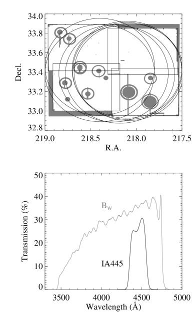
Figure 1.— The top panel shows our survey area. The photometric masks are shown in grey. The open squares represent the 4 pointings of the Subaru/SuprimeCam imaging using the $IA445$ filter. The open circles represent the field of views of 7 configurations of MMT/Hectospec observations. We trim the margins around the SuprimeCam fields by taking the box of R.A. ($\alpha=218.9^{\circ}-217.55^{\circ}$) and Decl. ($\delta=32.95^{\circ}-33.85^{\circ}$). The bottom panel shows the filter transmissions of the $IA445$ and $B_{W}$ filters, including all effects from atmosphere, telescope, and optics. We choose photometric LAE candidates using the color of these two filters. The observed comoving volume covered by the intermediate band survey is $82\times 66\times 187~{}h^{-3}$Mpc³.

II.1. Candidate Selection

We define a sample of LAEs at $z\approx 2.67$ using the following photometric criteria:

$$\{IA445<26\} \cap \{(IA445-B_{W})\leq-0.5\}$$ (1)

$$\cap \{(IA445-B_{W})\leq\frac{4}{9}(26-IA445)-0.9\}$$

$$\cap \{(B_{W}-R)\leq 0.8\}.$$

The bottom-left panel of Figure 2 shows the color-magnitude diagram of $IA445$ $-$ $B_{W}$ vs. $IA445$, for 10,000 randomly selected sources (grey points) from the total 242,678. The red solid lines represent our color selection described in Equation 1. The first two terms in Equation 1 represent magnitude and color limits. The last term of $B_{W}-R$ color rejects low redshift interlopers. From this photometric color selection, we extract 1957 LAE candidates; hereafter, referred to as pLAE. We show the spatial distribution of this pLAE sample, using black dots, on the top panel of Figure 2.

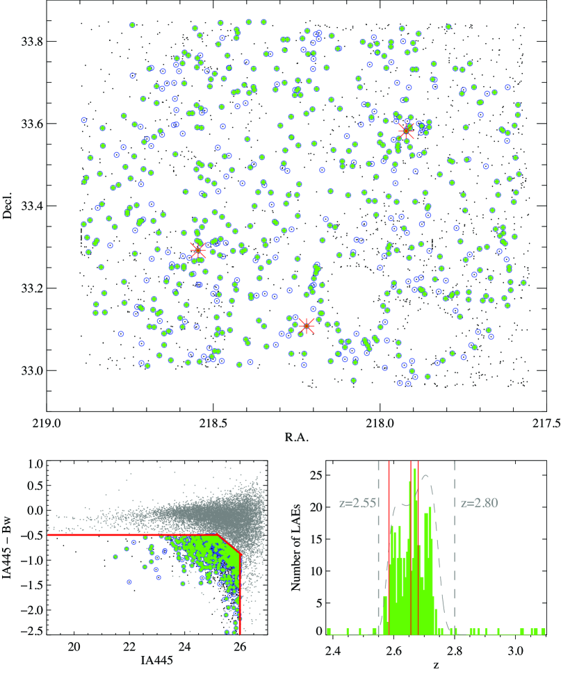
Figure 2.— The top panel shows the spatial distribution of 1957 photometric sample pLAE (black dots), 635 spectroscopically observed targets (blue open circles), and 434 redshift detections (green filled diamonds). The big (red) asterisks represent the three Lyman alpha blobs found in our survey field. The bottom-left panel shows the color-magnitude distribution, $IA445$ $-~{}B_{W}$ vs. $IA445$, for our source catalog (grey dots; $10^{4}$ objects are plotted from the total 242678 objects) and color selection criteria for pLAE (red solid lines). The same symbols of black dots, blue open circles, and filled diamonds are used for representing the same kinds of objects shown in the top panel. The bottom right panel shows the histogram of 434 redshifts (green bars) and filter transmission curve for $IA445$ (grey dashed curve). The two vertical dashed lines represent the redshifts, $z=2.55$ and $2.80$, respectively and three red solid vertical lines indicate the redshifts of three Lyman Alpha Blobs (LABs) discovered in our study.

II.2. Spectroscopic redshifts

We observed 635 candidates from the total 1957 pLAE sample using Hectospec, a multi-object spectrograph on the MMT telescope; the details about the spectroscopic data can be found in Hong et al. (2014). The seven large open circles in the top panel in Figure 1 show our 7 MMT/Hectospec pointings. Within our redshift selection box, $z=2.55-2.80$, we confirmed 415 spectroscopic LAEs from the observed 635 pLAE candidates (i.e., a success rate of 65%). We refer to this spectroscopically confirmed subset as zLAE. Extrapolating the success rate to the remaining photometric LAE sample using binomial trials, we expect a total sample of $1274\pm 17$ zLAEs out of the 1957 pLAE sample.

The bottom-right panel in Figure 2 shows the histogram of redshift detections for zLAE (green bars) and filter transmission curve for $IA445$ (grey dashed curve). The two vertical dashed lines represent the lower and upper redshift cutoffs, $z=2.55$ and $2.80$, respectively and three red solid vertical lines indicate the redshifts of three Lyman Alpha Blobs (LABs) discovered in our study. The top panel shows the spatial distributions of 635 spectroscopically observed targets (blue open circles), and 415 zLAE objects (green filled diamonds). The three red asterisks represent the locations of LABs, where their redshifts are $z=2.680,2.656,$ and $2.584$ respectively, in the order of increasing declination.

III. Statistics of Two-point Correlations

In this section, we investigate the spatial distribution of LAEs using two-point correlation functions by following the conventional clustering studies (e.g., Seljak 2000, Berlind & Weinberg 2002, Roche et al. 2002, Hamana et al. 2004, Zehavi et al. 2004, Zheng et al. 2005, Lee et al. 2006, Gawiser et al. 2007, Kovač et al. 2007, Lee et al. 2009, Ouchi et al. 2010, Geach et al. 2012, Sánchez et al. 2012).

III.1. Angular Correlation Function $\omega(\theta)$

We measure angular two-point correlation functions for the zLAE and pLAE samples using the estimator suggested by Landy & Szalay (1993; hereafter, the LS estimator),

$$\omega_{LS}(\theta)=\frac{DD-2DR+RR}{RR},$$ (2)

where DD is the pair count of observed sample, RR of random sample, and DR between observed and random samples, within the angular bin $(\theta-\delta\theta/2,\theta+\delta\theta/2)$. Since this estimator has been widely used, we only provide a brief description about this method. The details can be found in the papers cited above.

Figure 3 shows the measured angular correlation functions using the LS estimator for pLAE (black open squares; top) and zLAE (green solid circles; bottom). The error bars are calculated from bootstrap resampling (Ouchi et al. 2010). On the bottom panel, we also add the angular correlation function of pLAE using grey open squares for comparison with zLAE. The uncertainty of zLAE is larger due to the small sample size. In particular, the small scale clustering at $<20$″  is determined by a small number of close pairs. The green ‘x’ mark represents the two-point statistic when we remove the 3 LAEs from zLAEs near the largest LAB, LABd05, where we oversample in spectroscopy for investigating the environmental effect between LAB and LAEs. Overall, though the uncertainty of zLAE is large, the two angular correlation functions are consistent with each other.

The angular correlation function of the LAEs shows an inflection point at scales of 20″, corresponding to a comoving scale of $0.41h^{-1}$ Mpc. This distinct feature is predicted by halo occupation models, where it results from the transition from multiple galaxies occupying common halos to each galaxy occupying a single halo.

The LS estimator, $w_{LS}(\theta)$, in Equation 2 is a normalized quantity of its true angular correlation, $\omega(\theta)$, as

$$1+\omega_{LS}(\theta) = \frac{1+\omega(\theta)}{1+\omega_{\Omega}},$$ (3)

$$\omega_{\Omega} \equiv \frac{1}{\Omega^{2}}\int d\Omega_{1}d\Omega_{2}\omega(\theta),$$ (4)

where $\omega_{\Omega}$ is called “integral constant” (hereafter, IC). To retrieve the true angular correlation, $\omega(\theta)$, from our measured LS estimator, $\omega_{LS}(\theta)$, we need a method to correct this integral constant, $\omega_{\Omega}$. To estimate this IC, we rewrite Equation 3 and 4 in more practical forms as

$$\omega_{LS}(\theta) = \frac{\omega(\theta)-\omega_{\Omega}}{1+\omega_{\Omega}},$$ (5)

$$\omega_{\Omega} \approx \frac{\sum RR~{}\omega(\theta)}{\sum RR},$$ (6)

where Equation 5 is rewritten from Equation 3 and Equation 6 is a Monte Carlo integration of Equation 4 using the same random pairs, RR, in Equation 2 (Roche et al. 2002).

III.2. Interpretations from Single Power-law Correlation Functions

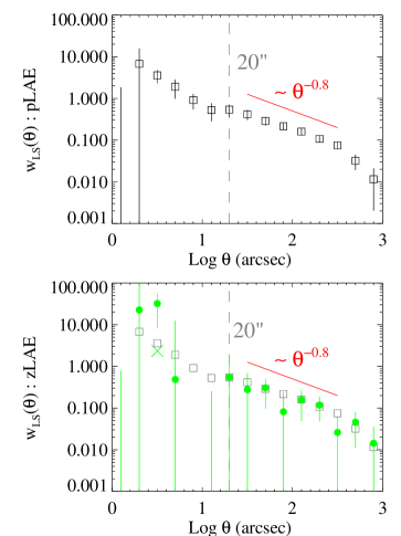
Figure 3.— The measured angular correlation functions for pLAE (black open squares; top) and zLAE (green solid circles; bottom), obtained using the LS estimator. The error bars are calculated from bootstrap resampling and represented by vertical lines. On the bottom panel, we also add the angular correlation function of pLAE using grey open squares for comparison with zLAE. Though the uncertainty of zLAE is large, both angular correlation functions are consistent, which implies that the final LAE sample with complete spectroscopic redshifts will not be much different from zLAE and pLAE.

III.2.1 Integral Constraint and Self-consistent Fit

Unfortunately, we cannot solve Equation 5 and 6, since $\omega(\theta)$ and $\omega_{\Omega}$ are coupled, and it is the LS estimator, $\omega_{LS}(\theta)$, what we can actually measure from galaxy distribution, not $\omega(\theta)$. We can resolve this coupling issue if we have some specific constraints on $\omega(\theta)$.

Conventionally, $\omega(\theta)$ has been assumed to follow a single power-law. In this case, we can solve the coupled equations as follows. First, we write down the equations as,

$$\omega(\theta) = A_{\omega}~{}\theta^{-\beta},$$ (7)

$$\omega_{\Omega} \approx \frac{\sum RR~{}A_{\omega}~{}\theta^{-\beta}}{\sum RR}.$$ (8)

If the two parameters, $A_{\omega}$ and $\beta$, are mathematically separable, Equation 8 can be rewritten as,

$$\omega_{\Omega} \approx A_{\omega}~{}R_{\Omega}(\beta),$$ (9)

$$R_{\Omega}(\beta) \equiv \frac{\sum RR~{}\theta^{-\beta}}{\sum RR},$$ (10)

where we refer to $R_{\Omega}(\beta)$ as “random pair function” (RPF). Defying the simple definition of RPF, there is a delicate divergence issue, which is described in Appendix A. The final result on the divergence is that RPF, $R_{\Omega}(\beta)$, is well-defined for $0\leq\beta<1$. In this valid $\beta$ range, the coupled equations can be rewritten as,

$$\omega_{LS}(\theta) = \frac{\theta^{-\beta}-R_{\Omega}(\beta)}{A_{\omega}^{-1}+R_{\Omega}(\beta)}.$$ (11)

Consequently, the problem of integral constraint is reduced to a self-consistent non-linear fit with the two parameters, $(A_{\omega}^{-1},\beta)$.

III.2.2 Best-fit Parameters and Real-space Correlation Lengths

Figure 4 shows the results of best-fit parameters for $\theta>20$″, based on the assumption of single power-law correlation. The left panels show the best-fit parameters for pLAE and zLAE, using Equation 11 with the RPFs. Instead of the conventional fiducial value of $\beta=0.8$, our nonlinear fits predict the slope near $\beta=0.6$. Hence, we also perform two other fits by fixing the slopes, $\beta_{fix}=0.8$ (middle panels) and $\beta_{fix}=0.6$ (right panels).

When the power-law shape of angular correlation function, $\omega(\theta)=A_{\omega}\theta^{-\beta}$, is known, we can also find its real-space clustering, $\xi(r)=(r/r_{0})^{-\gamma}$, using the Limber equation (Peebles 1980; Efstathiou et al. 1991),

$$\beta = \gamma-1,$$ (12)

$$A_{\omega} = Cr_{0}^{\gamma}\int_{0}^{\infty}F(z)D_{\theta}^{1-\gamma}(z)N(z)^{2}g(z)dz$$ (13)

$$\times \Big{[}\int_{0}^{\infty}N(z)dz\Big{]}^{-2},$$

where $D_{\theta}(z)$ is the angular diameter distance, $F(z)$ the redshift dependence of $\xi(r)$, $N(z)$ the redshift selection function from the zLAE sample, and

$$g(z) = \frac{H_{0}}{c}\Big{[}(1+z)^{2}(1+\Omega_{M}z+\Omega_{\Lambda}[(1+z)^{-2}-1])^{\frac{1}{2}}\Big{]},$$ (14)

$$C = \sqrt{\pi}\frac{\Gamma[(\gamma-1)/2]}{\Gamma(\gamma/2)}.$$ (15)

We summarize the best-fit parameters and related clustering lengths in Table 1. Overall, the parameter ranges of $A_{\omega}$ and $\beta$ are quite large, while the predictions of $r_{0}$ are relatively consistent as $r_{0}\approx 4h^{-1}$ Mpc. The large uncertainties on $A_{\omega}$ and $\beta$ arise from uncertainties in the power-law slope, which in turn are affected by a power-law being a poor representation of the observed angular correlation function (cf. the inflection point at 20″). As presented in Table 1, power-law fits with shallower or steeper slopes (i.e., $\beta=0.6,0.8$), result in smaller or larger clustering amplitudes (i.e., $A_{\omega}\approx 4-9$, at the consistent result of $\xi(r=4h^{-1}$Mpc$)=1$).

The measured clustering length, $r_{0}\approx 4h^{-1}$ Mpc, of the Boötes LAEs at $z=2.67$, is comparable to that derived for LAEs at $z=2.1$ (Guaita et al. 2010), H$\alpha$ emitters at $z=2.23$ (Geach et al. 2012), and the LBGs at $z\approx 3$ (Adelberger et al. 2005, Lee et al. 2006), and relatively larger than the LAEs from Gawiser et al. (2007) and Ouchi et al. (2010) at $z=3.1$. We summarize these comparisons in Figure 5. Overall, the Boötes LAEs show a similar or slightly larger clustering amplitude, compared to the previous studies.

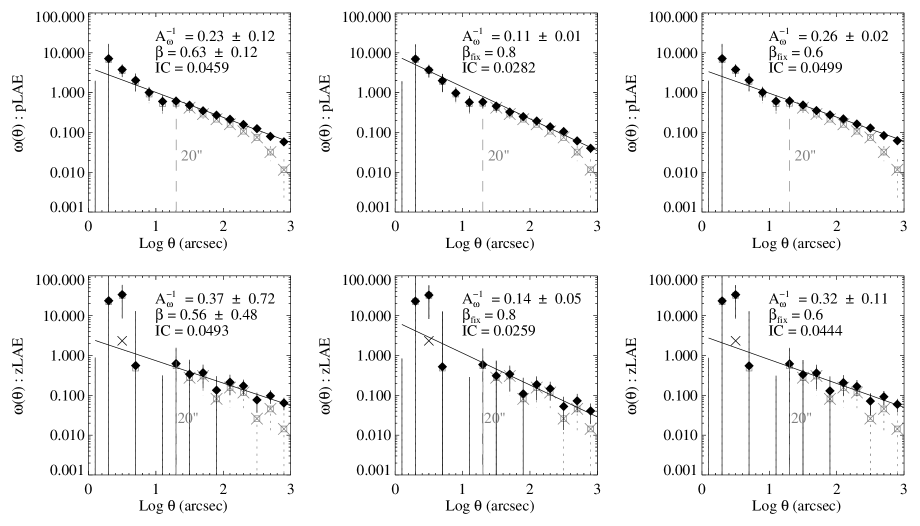
Figure 4.— The single power-law fits for pLAE (top) and zLAE (bottom) using the non-linear self-consistent fit in Equation 11 (left) and the fixed $\beta$ values with $\beta_{fix}=0.8$ (middle) and $\beta_{fix}=0.6$ (right). The results are summarized in Table 1.

Table 1Single Power-law Fits

Sample	$A_{\omega}$	$\beta$	$IC$	$r_{0}$
	(at 1 arcsec)			$h^{-1}$ Mpc
pLAE	$4.35^{+4.74}_{-1.49}$	$0.63\pm 0.12$	0.0459	$4.1^{+2.3}_{-0.9}$
	$9.09^{+0.91}_{-0.76}$	0.8 (fix)	0.0282	$4.1^{+0.2}_{-0.2}$
	$3.85^{+0.32}_{-0.27}$	0.6 (fix)	0.0499	$4.1^{+0.2}_{-0.2}$
zLAE	$2.70^{+\infty}_{-1.79}$	$0.56\pm 0.48$	0.0493	$3.6^{+\infty}_{-1.8}$
	$7.14^{+3.97}_{-1.88}$	0.8 (fix)	0.0259	$3.6^{+1.0}_{-0.6}$
	$3.13^{+1.64}_{-0.78}$	0.6 (fix)	0.0444	$3.6^{+1.1}_{-0.6}$

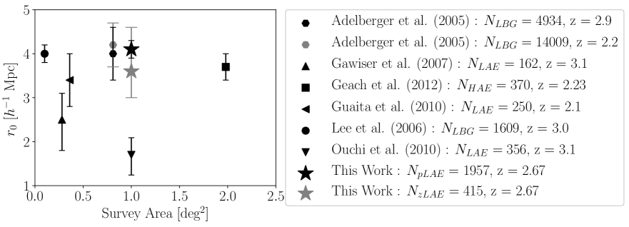
Figure 5.— The clustering length, $r_{0}$, vs. survey area for previous studies with similar redshifts. Overall, the Boötes LAEs show a comparable or slightly larger clustering amplitude, compared to the previous results.

III.3. Interpretations from Mean Halo Occupation Functions

In the previous section, we have assumed that the galaxy correlation function follows a single power law and measured the amplitude and slope by fits to the LAE pair distribution. Historically, this single power law assumption arises from two observations: (1) low redshift galaxies indeed show single power law clusterings in many cases, and (2), when a survey volume is small, clustering measurements at small scales are quite uncertain.

In the current paradigm of hierarchical galaxy formation and evolution, observed galaxy clustering (or, galaxy power spectra in $k-$space) can be reproduced analytically by using halo occupation distributions (HODs; e.g., Seljak 2000, Berlind & Weinberg 2002, Hamana et al. 2004, Zehavi et al. 2004, Zheng et al. 2005, Lee et al. 2006, Kovač et al. 2007, Lee et al. 2009, Ouchi et al. 2010, Geach et al. 2012). In this HOD formulation, galaxy clustering is generally scale-dependent, deviated from single power-laws, due to the non-linear bias in galaxy formation.

Although this analytic HOD formulation is advantageous to easily reproduce observed galaxy clustering analytically, along with intrinsic scale-dependent features, it relies on the assumption that the mean halo occupation only depends on the halo mass, and is valid when averaged over all halos. Effects other than halo mass are generally ignored in the HOD formulation. Since we find many $10^{11}M_{\odot}$ haloes in clusters, filaments, and outskirts around voids, it is not likely that all galaxies form in the same way in such different topological environments (Hong & Dey 2015, de Regt et al. 2018).

III.3.1 Halo Occupation Function

In this paper, we adopt the HOD from Geach et al. (2012), used for H$\alpha$ emitters at z=2.23. We refer the reader to Appendix B for details regarding this choice. The Geach et al. HOD is defined as follows:

$$N_{c}(M) = F_{c}^{B}(1-F_{c}^{A})\exp\Big{[}-\frac{\log(M/M_{c})^{2}}{2\sigma^{2}_{\log M}}\Big{]}$$ (16)

$$+ F_{c}^{A}\Big{[}1+\textrm{erf}\Big{(}\frac{\log(M/M_{c})}{\sigma_{\log M}}\Big{)}\Big{]},$$

$$N_{s}(M) = F_{s}\Big{[}1+\textrm{erf}\Big{(}\frac{\log(M/M_{1})}{\delta_{\log M}}\Big{)}\Big{]}\Big{(}\frac{M}{M_{1}}\Big{)}^{\alpha},$$ (17)

$$N_{g}(M) = N_{c}(M)+N_{s}(M),$$ (18)

where $N_{c}(M)$ represents the central distribution as a function of halo mass $M$, $N_{s}(M)$ the satellite distribution, and $N_{g}(M)$ the total galaxy counts, for a given halo mass, $M$. The central distribution is written using two terms: a Gaussian component centered at halo mass $M_{c}$ with the width of $\sigma_{\log M}$; and a smoothed step function component using an Error function with the smoothed length of $\delta_{\log M}$. $F_{c}^{A}$ and $F_{c}^{B}$ represent the duty cycle of central LAEs. The satellite distribution is written using the conventional power-law component with a tunable satellite’s duty cycle, $F_{s}$. Overall, the adopted HOD follows the conventional description of step function centrals and power law satellites, with additional flexibility in functional degrees of freedom.

When considering the complexity of halo occupations for emission line galaxies, we need to allow more flexible HODs for LAEs than typical galaxies, selected by broad-band photometry, traced by the longer lasting and more consistent emitting source, stars. However, over-flexible models inevitably overfit the data; hence, they cause degeneracy in possible interpretations. In the context of statistical learning, this is an inevitable trade-off between flexibility and interpretability of parametric model (James et al. 2013). Since we do not have definitive constraints on the HOD for LAEs, we will use the HOD from Geach et al. and accept all non-rejected HOD models as possible scenarios. In Appendix B, we present results from the conventional 3 parameters’ HOD (e.g., Zehavi et al. 2005) and discuss more about this trade-off issue.

Given the HOD, $N_{g}(M)$, we derive the galaxy number density, $n_{g}$, using the halo mass function, $n(M)$,

$$n_{g} = \int N_{g}(M)n(M)dM.$$ (19)

If we have a redshift selection function, $N(z)$, as shown in Figure 2, then we can take an effective average, $\langle n_{g}\rangle$, over the selection function as,

$$\langle n_{g}\rangle = \frac{\int n_{g}(z)N(z)(dV/dz)dz}{\int N(z)(dV/dz)dz}.$$ (20)

We measure $\langle n_{g}\rangle=2.50\pm 0.05\times 10^{-4}h^{3}~{}\textrm{Mpc}^{-3}$ from the $1274\pm 17$ LAEs, extrapolated using the current yield fraction 65% from 1957 LAE candidates, based on the binomial trials. We use the PYTHON package, halomod (Murray et al. 2013), for HOD calculations with the cosmological parameters from Planck13  in ASTROPY and adopt the halo mass function from Tinker et al. (2008).

III.3.2 The Best-Fit Parameters : Inverse Correction of Integral Constant

Our adopted HOD has 8 parameters, $M_{c},M_{1},\alpha,F^{A}_{c},F^{B}_{c},F_{s},\sigma_{\log M}$, and $\delta_{\log M}$. Generally, the smoothing scales of step function terms, $\sigma_{\log M}$, and $\delta_{\log M}$, are not as critical to the shape of the resulting angular correlation function as $\alpha,M_{1}$, and $M_{c}$. This means that $\alpha,M_{1}$, and $M_{c}$ are well constrained by the angular correlation measurement, whereas the others are not. Bayesian samplings can provide quantitative information, about how well the observed angular correlation function can constrain each parameter, by studying the posterior probability density function (PDF) as shown in Figure 6.

Among the 8 parameters, we first fix one of the least important parameters, $\delta_{\log M}\equiv 1$, which controls the width of error function in Equation 17. Since $\sigma_{\log M}$ is used in both Gaussian and Error functions in Equation B13, we do not fix this parameter to allow the Gaussian width to vary. From the density normalization of Equation 20, $M_{c}$ can be determined using $\langle n_{g}\rangle=0.0025~{}h^{3}~{}\textrm{Mpc}^{-3}$ . Therefore, our final HOD has the 6 free parameters, $M_{1},\alpha,F^{A}_{c},F^{B}_{c},F_{s},\sigma_{\log M}$.

As we have pointed out in §III.1, IC can be determined only by its true angular correlation function. For single power-law correlations, we can resolve this IC problem using the non-linear fit with random pair function in Equation 11.

In the HOD formulation, we can resolve this issue using the inverse correction of integral constraint as follows. First, we have a well-defined model prediction of the angular correlation function, $\omega_{HOD}(\theta)$, from a given HOD. Since this is a true angular correlation function, not degraded by survey volume, we can calculate its corresponding IC, $\omega_{\Omega}$, directly from $\omega_{HOD}(\theta)$ :

$$\omega_{\Omega} \approx \frac{\sum RR~{}\omega_{HOD}(\theta)}{\sum RR}.$$ (21)

From $\omega_{\Omega}$, we define a new inverse HOD angular correlation function, $\tilde{\omega}_{HOD}(\theta)$, as :

$$\tilde{\omega}_{HOD}(\theta) \equiv \frac{\omega_{HOD}(\theta)-\omega_{\Omega}}{1+\omega_{\Omega}}.$$ (22)

This inversely corrected HOD function, $\tilde{\omega}_{HOD}(\theta)$, is now directly comparable to the observed LS estimator, $\omega_{LS}(\theta)$. Therefore, we can write down the correct $\chi^{2}$ as

$$\chi^{2}(M_{1},\alpha,F^{A}_{c},F^{B}_{c},F_{s},\sigma_{\log M})$$

$$=\sum_{i}\frac{\big{[}\omega_{LS}(\theta_{i})-\tilde{\omega}_{HOD}(\theta_{i})\big{]}^{2}}{\sigma^{2}_{LS}(\theta_{i})}$$ , (23)

where $\theta_{i}$ represents each angular bin and $\sigma^{2}_{LS}$ the bootstrap sampling variance of LS estimator. Finally, we define the likelihood function as

$$\ln\mathcal{L} = -\frac{1}{2}\chi^{2}.$$ (24)

III.3.3 Results : Degeneracy in Two–point Statistics

We use two different methods to obtain best-fit HOD parameters, (1) one from $\chi^{2}$ minimization, referred to as Model#1, and (2) the other from Bayesian posterior probability density function (PDF), referred to as Model#2, obtained using the Markov chain Monte Carlo (MCMC) sampler, emcee (Foreman-Mackey et al. 2013).

Figure 6 shows the result of posterior PDF, obtained using the MCMC sampler, emcee. We put 120 walkers in total (i.e., 20 walkers for each parameter) and iterate 950 steps. We discard the early 450 steps as burn-in and take 500 steps to retrieve the posterior PDF. This 6 dimensional posterior PDF is visualized in contours (2D marginalized probabilities) and histograms (1D marginalized probabilities). The median value and $\pm 1\sigma$ errors for each parameter from the 1D marginalized histograms are listed in Table 2. Since the marginalized distributions for $F_{s}$ and $\sigma_{\log M}$ are flat and bimodal respectively, it is not informative to present the medians and errors for these parameters. To interpret the posterior PDF, $\log_{10}M_{1}$ is the only parameter, well constrained by the angular correlation function. The others are marginally (or poorly) constrained. This is not a surprising result when considering the relatively large number of free parameters compared to the conventional 3 parameters’ HOD. Though there are many other statistics such as Minkowski functionals, genus, percolation threshold and higher order correlation functions, the current HOD formulation only fits the abundance and two-point statistic of observed populations. Hence, the degeneracy in HOD models is inevitable if the number of free parameters exceeds the constraining power of abundance and two-point correlation; i.e., if the HOD function is over-flexible.

The posterior PDF provides a better statistical interpretation for the best fit model than other methods such as maximum likelihood or least chi-square. However, since the least chi-square method is widely used, we also compute it; hence, Model#1, using the Nelder-Mead method implemented in the PYTHON/SCIPY package. From various initial positions, we obtain the consistent output of Model#1. However, we cannot reject the possibility that Model#1 is derived from a local minimum. We take, therefore, Model#1 as one of many possible selections, statistically allowed within the posterior PDF. The blue points and dotted lines in Figure 6 represent the location of Model#1 in the parameter space. Though this location is less likely in the posterior PDF, this location in parameter space is not ruled out by the MCMC approach.

From the 2D contours in Figure 6, we select a more likely position, Model #2, represented by the red points and solid lines. A major difference between Model#1 and Model#2 comes from the parameter, $\sigma_{\log M}$ , which shows the bimodal histogram. Model#1 is selected from the minor bump, while Model#2 from the major bump. These Bayesian selections contrast with the different reduced chi-square values, $\chi^{2}/\nu=0.51$ for Model#1 and $\chi^{2}/\nu=1.2$ for Model#2. Model#1 is a preferred choice, therefore, in the least chi-square method, whereas Model#2 in the Bayesian method. The is issue is that neither model is rejected by the tests in abundance and two-point statistic, though their HODs are significantly different.

Figure 7 shows the angular two point correlation functions (left) and halo occupation distributions (HODs; right) for Model #1 (blue) and Model #2 (red). The dotted grey line represents the angular dark matter correlation function (Takahashi et al. 2012) and we measure the bias, $b_{LAE}=2.2^{+0.2}_{-0.1}$, at scales larger than 10″. This is slightly larger than, but still consistent with that found by previous works ($b\approx 1.5-2.0$; Gawiser et al. 2007, Guaita et al. 2010, Ouchi et al. 2010, Lee et al. 2014). In the left panel, each dashed line represents the two point function from each HOD Model without the effect of survey volume size and each solid line the inversely corrected two point function using our inverse integral constraint method. After this inverse correction, the observed clustering points from the LS estimator (black solid circles with error bars) can be directly comparable to the solid line; i.e., we can use the LS estimator as a direct observable without any further correction. In the right panel, the dashed, dotted and solid lines represent the expected number of central, satellite and total galaxies, respectively.

In this figure, Model#1 and Model#2 show very different HODs, especially in the central galaxy populations. For Model#1, the central LAEs are mostly occupied in a very narrow halo mass range, centered at $\log_{10}M_{c}=11.6$ with the Gaussian width of $\sigma_{\log M}=0.097$. At its peak, the occupation fraction, $<N_{g}>$, reaches 93%. This drops rapidly as the halo mass increases or decreases away from this peak halo mass. For massive halos over $10^{12}h^{-1}M_{\odot}$, the central LAE occupations become less than 0.3%. Therefore, most of LAEs found in these massive halos should be satellites in this Model#1 scenario; hence, we refer to this as, namely, “Dead Core Scenario” or “Dusty Core Scenario”. The lack of central LAEs at halo masses $>~{}10^{12-13}$ in Model#1 may imply that central galaxies in these halos do not produce much Ly$\alpha$ emission, either because they are more rapidly quenched or that they are dustier on average; hence, dead or dusty cores.

On the other hand, for Model#2, the central LAEs are distributed over a broad range of halo masses, centered at $\log_{10}M_{c}=12.40$ with the Gaussian width of $\sigma_{\log M}=0.63$. At this Gaussian peak, the occupation fraction is 31%, which is much lower than the dominant 93% from the Dead Core Scenario. For massive haloes, even larger than $10^{13}h^{-1}M_{\odot}$, the central occupation fractions are above 20% in Model#2. We refer to this as “Active Core Scenario” or “Pristine Core Scenario”, suggesting that the central galaxies in massive halos are still less contaminated by dust, actively emitting Ly$\alpha$ photons, unlike the dead or dusty cores from Model#1.

Consequently, Model#1 and Model#2 suggest very different scenarios about the formation and evolution of LAEs at $z\approx 2.67$. We cannot discern which scenario is more reliable for the observed LAEs at $z\approx 2.67$. To resolve this issue, we need to resort to higher order correlations, which in turn are limited by the sample statistics.

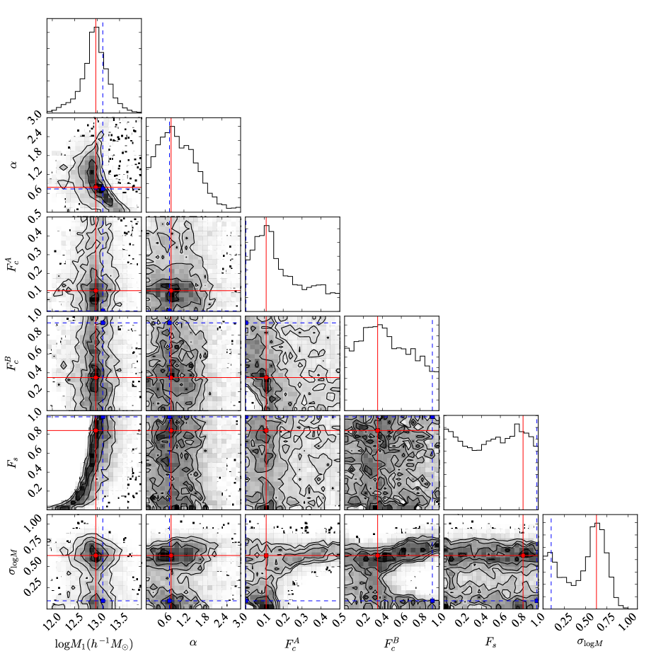
Figure 6.— The posterior probability density function from the MCMC run. This 6 dimensional posterior probability density function is visualized in contours (2D marginalized probabilities) and histograms (1D marginalized probabilities). The blue points and dashed lines represent the parameters selected from the least chi-square method (Model#1), and the red points and solid lines selected from the posterior probability function (Model#2). The parameters are summarized in Table 2.

Table 2The Parameters of Halo Occupation Functions

Name	$\log_{10}M_{1}$	$\alpha$	$F^{A}_{c}$	$F^{B}_{c}$	$F_{s}$	$\sigma_{\log M}$
Model#1	13.13	0.74	$2.9\times 10^{-3}$	0.93	0.99	$9.7\times 10^{-2}$
Model#2	12.97	0.79	0.11	0.35	0.84	0.63
Posterior PDF	$12.95^{+0.26}_{-0.29}$	$0.94^{+0.69}_{-0.56}$	$0.14^{+0.21}_{-0.09}$	$0.43^{+0.34}_{-0.27}$	flat	bimodal

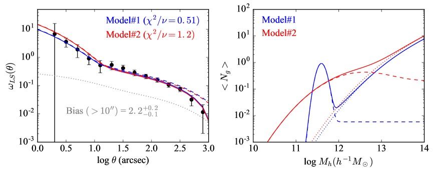
Figure 7.— The two point correlation functions (left) and halo occupation distributions (HODs; right) for Model#1 (blue) and Model#2 (red). The dotted grey line represents the angular dark matter correlation function (Takahashi et al. 2012). On the left panel, each dashed line represents the true two point function from each HOD Model without any effect of survey volume size and each solid line the inversely corrected two point function using our inverse integral constraint method. In the right panel, the dashed, dotted and solid lines represent the expected number distributions of central galaxies, satellite galaxies and the total, respectively. The two models, Model#1 and Model#2, show very different HODs, but both predict similar two-point correlation functions, matching the observed clustering in the accuracy of practical studies; or, at least, both are not statistically rejected in the test of two-point statistics.

IV. Statistics of Network Topology

In the previous section we have presented measurements of the two-point correlation function and abundance of LAEs. The measurements are fit by two HOD models which predict the same abundance and two-point correlation within the uncertainties. However, their HODs are very different, especially in the central galaxy populations. This is an evident degeneracy in two-point statistics.

In this section, we use network science tools to investigate the topological structures of the observed LAEs (Observed LAEs), and compare these with the topologies generated by the two best-fit HOD models (Model#1 and Model#2) and random spatial distributions (Random Model). From the statistics of network topology, we show that both Model#1 and Model#2 fail to explain the spatial distribution of observed LAEs; hence, the topological structures of observed LAEs are different from the HOD models’ predictions. This indicates that the assumption of constant halo occupation for all halos of a given mass is too simple to be applicable, at least, to LAEs.

IV.1. Generating Networks from Galaxy Point Distributions

We generate 60 mocks for each HOD model by populating LAEs using the halo catalog from Small MultiDark Planck simulation (SMDPL; Klypin et al. 2014) and projecting them on the sky mask, shown in Figure 1. Central galaxies are randomly placed in parent haloes given by the HOD. Likewise, satellite galaxies are placed in their sub-haloes to match the target occupation. Note that our catalog allows for satellites to be placed in parent haloes that may or may not host a central galaxy.

A single mock catalog matches the area of the survey. The depth is given by the $IA445$ filter transmission curve, which defines a redshift and comoving distance range where the Ly$\alpha$ line falls inside the filter. Then, multiple mock catalogs are extracted from the simulation volume with no overlapping. The different number of galaxies and clustering in each of the mocks is thus a result of cosmic variance.

For observed LAEs, we have measured the redshifts of 635 candidates from the total 1957 pLAEs. For the rest of 1322 photometric candidates, since the current yield fraction is 65%, we generate a binomial ensemble with 300 realizations for considering the incompleteness of our spectroscopic followup. This ensemble size is large enough to show asymptotic behaviors in graph statistics; i.e., no quantitative differences in graph statistics by taking larger ensemble sizes. In §IV.2, we will present the details about this binomial convergence. Finally, as a basic comparison set, we generate 60 random point distributions as Random Model.

From each spatial distribution, we build a network using the conventional Friends-of-Friends (FOF) recipe (Huchra & Geller 1982, Hong & Dey 2015, Hong et al. 2016) for a given linking length $l$, where the adjacency matrix is defined as,

$$A_{ij}=\left\{\begin{array}[]{ll}1&\textrm{ if }r_{ij}\leq l,\\ 0&\textrm{ otherwise, }\end{array}\right.$$ (25)

where $r_{ij}$ is the distance between the two vertices (i.e., galaxies), $i$ and $j$. This binary matrix quantitatively represents the network connectivities of the FOF recipe. Many important network measures are derived from this matrix. Interested readers are directed to Newman (2003), Dorogovtsev, Goltsev & Mendes (2008), and Barthélemy (2011) for further information.

Figure 8 shows the histogram of the number of galaxies, $N_{galaxy}$, for each model composed of 60 mocks; Observed LAEs (red), Random Model (grey), Model#1 (green) and Model#2 (blue). For a proper comparison, we take 60 binomial samples from the total 300 realizations for this histogram; though no qualitative difference in abundance statistics between 60 and 300 binomial realizations. The variances of $N_{galaxy}$ for Model#1 and Model#1 are due to cosmic density fluctuations, confined by the size of survey volume. Observed LAEs are shown at a range of possible abundances estimated using the known photometric uncertainties and spectroscopic completeness, which suggest an LAE abundance in the field of 1274$\pm$17. Finally, the variance for Random Model is Poissonian, a comparable random reference to the other models.

The cosmic variances of Model#1 and Model#2 are much larger than the binomial variances of Observed LAEs and Random Model. We, therefore, expect the network properties of the observed LAEs to be contained within the range exhibited by the HOD mocks.

IV.2. Results : Implications from Network Statistics

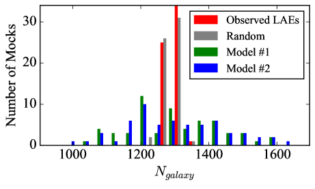
Figure 8.— The histogram of the number of galaxies, $N_{galaxy}$, for each model, composed of 60 mocks; Observed LAEs (red), Random Model (grey), Model#1 (green) and Model#2 (blue). The cosmic variances of Model#1 and Model#2 are much larger than the binomial variances of Observed LAEs and Random Model. Naively, due to this dominance of cosmic variance, we may expect that the network statistics from Observed LAEs are fully embedded within the cosmic variances of the HOD mocks.

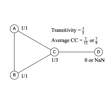
Figure 9.— The graph schema demonstrating the meanings of transitivity and average clustering coefficient (Average CC). In this graph, we can find 5 triplets (i.e., 5 $\vee$ configurations), 3 from the ‘ABC’ triangle and the other 2 from the “Y” shape, connected from the vertex ‘D’ with the pivot center ‘C’. Among these 5 triplets, three of them on the ‘ABC’ triangle are closed. Hence, the transitivity of this graph is $\frac{3}{5}$. The clustering coefficient is a transitivity-like quantity, but assigned to each vertex. For example, the vertex ‘C’ has three neighbors, ‘A’, ‘B’, and ‘D’; hence, 3 $\vee$ configurations, centered on ‘C’. In general, for a vertex with $k$ neighbors, $\frac{k(k-1)}{2}$ triplet combinations exist. Since only ‘A’ and ‘B’ vertices are connected among the three triplets, the clustering coefficient for ‘C’ is $\frac{1}{3}$. Similarly, 1 is the clustering coefficient for each of ‘A’ and ‘B’. For a vertex with $k<2$ neighbors, we cannot define a clustering coefficient since the denominator is zero. In this case, to the vertex, we can assign (1) 0 or (2) not-a-number (NaN). For the former, the vertex ‘D’ is counted when averaging all clustering coefficients, resulting in the Average CC $=\frac{7}{12}$, while, for the latter, ‘D’ is excluded, the Average CC $=\frac{7}{9}$. In this paper, we choose the latter definition to assign NaNs to all vertices with $k<2$ neighbors.

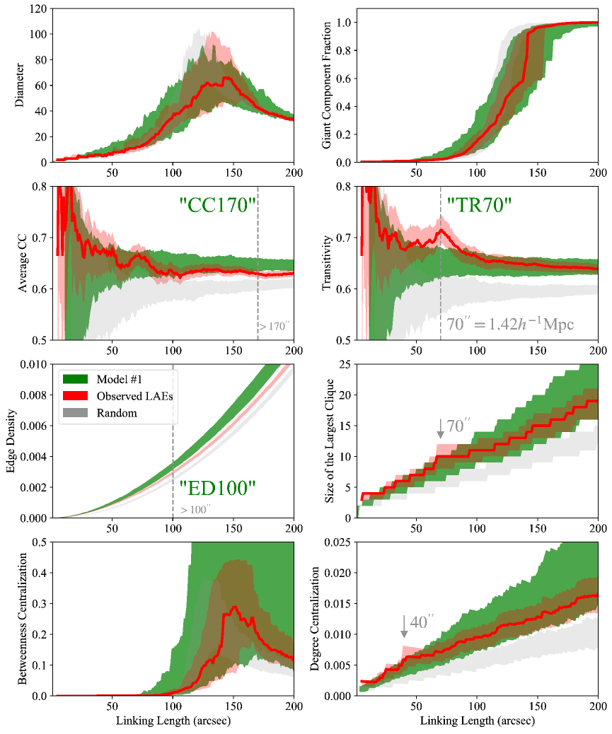
Figure 10.— The network measurements for Model#1 (green), observed LAEs (red), and random point distributions (grey); diameter (top-left), giant component fraction (top-middle), transitivity (top-right), average clustering coefficient (middle-left), edge density (center), size of the largest clique (middle-right), betweenness centralization (bottom-left), closeness centralization (bottom-middle), and degree centralization (bottom-right). See the text for details.

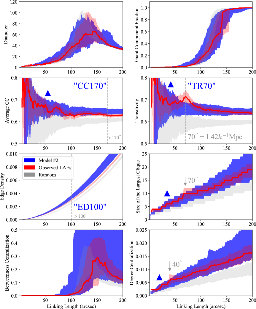
Figure 11.— The same with Figure 10 for Model#2 (blue), observed LAEs (red), and random point distributions (grey). The 4 blue solid triangles indicate the regions of improved statistics by Model#2. The major difference between Model#2 and Model#1 is the higher fraction of central galaxy occupation in massive halos (see Figure 7).

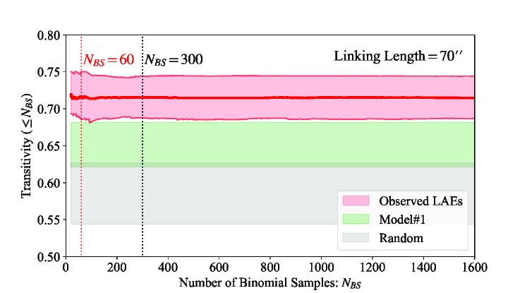
Figure 12.— The transitivity measurements vs. the number of binomial samples, $N_{BS}$, at the linking length of $70\arcsec$, for Observed LAEs (red shaded area); hence, a test of the convergence of binomial sampling about the anomaly “TR70”. The central thick line represents the 50 percentile (median) and the others 5 and 95 percentiles. The red shaded range at $N_{BS}=300$ (dotted black vertical line) is what is shown at $70\arcsec$ in Figure 10. For comparison, we also plot the ranges of transitivities for Model#1 (green) and Random Model (grey) at $70\arcsec$ with the same colors shown in Figure 10. For $N_{BS}\geq 300$, the transitivity measurements show saturated asymptotic behaviors. Even for $N_{BS}=60$, no qualitative differences can be found from the larger sampling sizes for $N_{BS}\geq 300$.

For various angular linking lengths from 0″  to 200 ″, we build a series of FOF networks for each spatial distribution. Then, for each network, we measure 8 network quantities: diameter, giant component fraction, average clustering coefficient (average CC), transitivity, edge density, size of the largest clique, betweenness centralization, and degree centralization. We present the definitions of these 8 quantities in a separate section, Appendix C, so as not to distract the reader from the main thread of this paper.

Figures 10 and 11 show the results of network statistics for the Observed LAEs, Model#1, Model#2, and Random Model, as a function of the linking lengths. Among 60 realizations for each model (300 realizations for Observed LAEs), we remove 5% outliers on both top and bottom regions. Therefore, each colored region represents 90% of its statistical distribution. For Observed LAEs, as a likely position for the case of complete spectroscopic selection, we plot the median position, using the red solid line.

To test the reliability of binomial sampling for handling the incomplete spectroscopic survey, we measure transitivity values for various numbers of binomial sampling. Figure 12 shows the transitivities vs. the number of binomial samples, $N_{BS}$, at the linking length of $70\arcsec$ for Observed LAEs (red shaded area). Notably, the transitivities show asymptotic behaviors for $N_{BS}\geq 300$; hence, no further variations for larger sampling sizes. Even for $N_{BS}=60$, there is no qualitative difference from the case of $N_{BS}=300$. We think that this is because the randomness of binomial sampling affects the graph statistics severely and directly. As shown in Figure 8, the variance of abundances for Observed LAEs is quite smaller than the HOD mocks. However, the variances of graph statistics for Observed LAEs are not much different from the HOD mocks even for tens of binomial realizations as shown in Figure 12. Hence, though there are $2^{1322}$ kinds of binary permutations (detected or non-detected LAEs) for unexplored photometric candidates, the random selections by binomial sampling shuffle the outputs quite enough to show the asymptotic statistical behaviors in graph measurements for $N_{BS}\geq 300$. We note that this argument is only valid when the best guess of complete spectroscopic survey is to extrapolate the current yield to the rest of unexplored photometric candidates. We assume that this extrapolation is a practically reasonable approach with the currently available pieces of limited information.

From the results of network statistics, we obtain the 4 main implications below.

IV.2.1 Both HOD models fail to explain the graph topology of observed LAEs

In Figure 10, we find that the comparison of network measures computed from the observed data with those computed from the mocks results in the following three main differences : (a) the transitivity curve of the observed data shows a “feature” at a scale of $\approx$70″ (1.4 $h^{-1}$ Mpc comoving) which is not present in the mocks, and which is not observed in the average CC (hereafter, we refer to this anomalous feature as TR70); (b) the average CC curve of the observed data at scales $>$170″ (3.4 $h^{-1}$ Mpc comoving) is lower than that computed for the mocks (hereafter, CC170); and (c) the observed edge density curve at scales $>$100″ is not reproduced by the mocks (hereafter, ED100). Roughly, average CC and transitivity are biased and unbiased triangle densities respectively. Figure 9 shows a schema demonstrating the meanings of these triangular statistics. Edge density is a connection (or, friendship) density, dividing the number of edges by the total number of pair-wise combinations. We discuss each of these anomalies in more detail below.

TR70 is the most conspicuous anomaly in the 8 panels of Figure 10. Near 70″, the transitivity of observed LAEs is much higher than the predictions of HOD mocks. The boundaries of the shaded regions shown for the models and observed LAEs represent the 5% outliers. Hence, there is $<0.25$% (5% $\times$ 5%) chance that this observed feature can be reproduced by Model#1; or over $99.75$% chance to reject Model#1 . In addition, this TR70 feature is not likely to be a result of the image mask, since it is not seen in the transitivity curves constructed from the mocks, to which the same mask is applied.

The angular scale of 70″ corresponding to 1.4$h^{-1}$ Mpc in the comoving scale is smaller than the typical scales for proto-clusters (Chiang et al. 2013, Orsi et a. 2016), but still larger than most of single halo scales. Hence, the transitivity excess at this intermediate scale suggests a strong intergalactic interaction in the formation of LAEs in this field. We explore this strong environmental effect in more details in a separate section with the additional network statistics of clique and centralization.

For linking lengths greater than 170″, the average CCs of Observed LAEs are lower than the Model#1’s predictions. The average CC is biased to the majority’s CC value, while the transitivity is a network-wise unbiased triangle density. In our Boötes LAEs, field LAEs are the majority, since group LAEs are rare. Small neighbors of field LAEs, hence, dominate the average CC statistic.

Unlike the feature TR70 seen in the transitivity curve, the average CC measurement does not show a significant anomaly at a scale of 70″. This suggests that the TR70 anomaly is not likely to be caused by the majority of field LAEs but instead by the LAEs in group environments, which are a minority of the observed population. Near 70″, therefore, the HOD mocks seem to reproduce the triangular configurations for field LAEs, the majority, but fail when including the minority, group LAEs. In other words, something interesting happens in group LAEs near 70″, which cannot be reproduced by the HOD formulation.

In contrast, the transitivity measure is consistent with the HOD prediction at scales $>170$″, whereas the average CC is not. This indicates that the observed LAEs and HOD mocks are consistent in the network-wise triangle densities at $>170$″, but the HOD mocks overpredict the average CC values at these scales. Namely, the observed field LAEs are less triangular than the HOD mocks in the local clustering configurations at $>170$″. It is not straightforward to determine which topological configuration causes this feature. One possible interpretation is that the observed field LAEs have more obtuse angles in triple configurations (i.e., $\vee$) than the HOD mocks. These more obtuse configurations can decrease the local CCs. As a trade-off, the observed LAEs in group environments need to have more triangular configurations, since the transitivity still needs to be consistent with the HOD mocks at $>170$″. Hence, our possible interpretation of CC170 is that the real observed LAEs are less triangular with more obtuse angles in spatial alignments of the field environments but more triangular in the group environments than the HOD mocks; more strained and stretched in field LAEs and more balled and compact in group LAEs than the HOD mocks.

For the edge density measurements, the HOD mocks overpredict the number of edges at most scales. Along with TR70, this is an additional evidence that the HOD mocks fail to reproduce the topology of observed LAEs. The difference in edge densities is more visible for $>100$″. Hence, we refer to this anomaly as ED100. Since edge is a basic structure, many factors can affect this count of connections. The less triangular configuration in field LAEs, mentioned above for interpreting CC170, can be one of such factors to lower the edge density than the HOD mocks.

In Figure 11, Model#2 seems to match the network statistics better than Model#1, but the three major anomalies are still not resolved by Model#2. Therefore, both HOD models fail to explain the real graph topology of observed LAEs. When considering the simplicity of mean halo theory, the HOD mocks explain relatively well the overall topological features of observed LAEs, only failing at certain scales. In contrast, the random point distribution fails at most scales in most statistics.

Overall, the anomalies found in network statistics suggest that the HOD mocks fail in the topological tests of network statistics; or, if the HOD formulation is right, the Boötes LAEs are a very special outlier in the cosmic variance, showing very abnormal environmental effects. We note that we have only shown the failures of two specific HOD models in graph statistics. This could be a suggestive evidence that the current HOD formulation needs to be improved for explaining (especially) the populations depending on environments strongly, but not a definitive evidence to deny the whole HOD framework.

IV.2.2 The Boötes LAEs are not a good filament/wall tracer

In Figures 10 and 11, the 8 panels can be divided into two groups; (1) diameter, giant component fraction, betweenness centralization, and (2) average CC, transitivity, edge density, size of the largest clique. The network measures in the first group show no significant statistical differences between the observed LAE sample and the other models. In contrast, the second group of measures do show differences, as described in the previous section. We note that the first group reflects the global pathway structures while the second group the local configurations as their definitions indicate, described in Appendix C.

The observed LAEs and HOD mocks are different in the local topology from random networks, while, in the global topology, the HOD mocks seems to even overwhelm the random networks in variance. The latter point seems confusing; especially, considering the results of our previous study (Hong et al. 2016), which demonstrates that simulated galaxies and Lévy flights show very different topology not only locally but also globally.

This may be due to the transient property of LAEs, having a specific duty cycle. For the work of Hong et al. (2016), we selected all simulated galaxies with stellar masses greater than $10^{8}$ M_⊙; hence, more likely to trace underlying filamentary structures than transient LAEs. The HOD recipe of probabilistic occupations on dark matter halos also can add more stochastic fluctuation to the mock LAEs. Analyzing the two-dimensional projection of the large scale distribution also dilutes and distorts the signal (the data analyzed in Hong et al. 2016 used the full 3-d distribution).

Consequently, though the observed and mock LAEs show many distinct local features, the global large-scale structures such as filaments or walls are not well characterized in the 2-dimensional projection of the LAE distribution and will require the complete redshift distribution for proper analyses.

IV.2.3 Strong environmental effect on the formation and evolution of LAEs

In this section, we investigate which topological configuration may be responsible for TR70. There are many graph structures, which can increase transitivity. One of them is a clique. As explained in Appendix C and shown in Figure C2, a clique is a complete subgraph, and galaxy groups and clusters form cliques in galaxy FOF networks. Therefore the abnormal excess in triangular configurations, TR70, can be related to clique statistics.

To test this idea, we measure the size of the largest clique, shown in the right panels of the third row in Figures 10 and 11. The excess of the largest clique size is also found at 70″, though its statistical significance is not as strong as TR70. The second, third, and next largest cliques also contribute to the transitivity, though they are not traced by this measurement. Hence, this suggests that TR70 is due to the larger clique sizes in the observed LAEs than in the HOD mocks. The median of the HOD mocks predicts that 7 LAE should inhabit the largest clique; the observed distribution shows 10, suggesting that scale sizes of 1.4$h^{-1}$ Mpc contain $\sim$43% more LAEs than predicted by the mocks. TR70 may therefore indicates a strong environmental effect on the formation and evolution of LAEs at $z\approx 2.67$, exerted within the scale of $1.4h^{-1}$ comoving Mpc (at least for the LAEs within this dataset).

If we find a clique excess at a certain scale, we can also expect some related feature in centralization measurements. Figure C3 in Appendix C shows the three graph schemata, ring, star, and clique, with 7 vertices. These schemata demonstrate that a star graph becomes a clique when we double the linking length. We refer to this as star-clique transition in spatial FOF networks. In more complex real-world networks, the transition may not be as clearly visible as Figure C3 demonstrates. However, the transitional feature can be detected statistically in the centralization measurements at the half scale of the clique feature. The bottom-right panels in figures 10 and 11 show the centralization measurements of degree centrality. Both the degree centralization and largest clique size curves show similar “knee” features at scales of 40″and 70″ respectively. In contrast, the HOD mocks only show featureless linear trends. This indicates that the Boötes LAEs have statistically more star-like configurations at 40″  and the larger size of the largest clique at 70″  than the HOD mocks, implying the star-clique transition in the network of Boötes LAEs.

We have found two interesting clues of the star and clique configurations at 40″  and 70″  respectively. Though not as strong as TR70, these two features imply that TR70 is due to the larger clique sizes of observed LAEs than the HOD mocks, which in turn may suggest an environmental factor in the formation and evolution of LAEs at $z\approx 2.67$.

IV.2.4 Model#2 is marginally preferred over Model #1

Finally, we compare the differences between Model#1 and Model#2. In all 8 measurements, Model#2 shows better matches with the observed LAEs than Model#1, though no special improvements can be found for explaining the three anomalies, CC170, TR70, and ED100, for Model#2 either. The major improvements of Model#2 from Model#1 are marked using the solid blue triangles in Figure 11. The local statistics of average CC, transitivity, size of the largest clique, and degree centralization are larger in Model#2 than in Model#1 due to the higher fraction of central galaxy occupation, which we have referred to as “Pristine Core Scenario”. These increased local statistics fit better the topology of observed LAEs.

Hence, the network statistics prefer Model#2 of the “Pristine Core Scenario” that, at $z\approx 2.67$, the central galaxies in massive halos, $>10^{12}h^{-1}M_{\odot}$, still need to be less dusty to emit Ly$\alpha$ photons, potentially due to some replenishing channels of pristine gas such as the cold mode accretion (e.g., Kereš et al. 2005; Dekel & Birnboim 2006; Kereš et al. 2009).

V. Summary and Discussion

We have investigated the spatial distribution of LAEs at $z\approx 2.67$, using the two-point correlation function and network statistics. From single power-law fits, we measure the correlation length, $r_{0}=4h^{-1}$ Mpc, and bias, $b_{LAE}=2.2^{+0.2}_{-0.1}$, consistent with previous studies of LAEs at similar redshifts. The power-law slopes are more uncertain and less consistent than the measured correlation lengths due to the clearly visible inflection point in the observed correlation function at small scales; i.e., where the one-halo term of subhalo statistics dominates. To obtain more accurate two-point statistics at these small scales reflecting the halo substructure, we need a larger survey volume containing better statistics on the small-scale separations (i.e., at $<10$). Many current and future surveys will provide more accurate small-scale statistics so that we can investigate the scale-dependent features in two-point statistics beyond the single power-law interpretations.

From the HOD analysis, we have obtained two disparate, but degenerate, models, Model#1 and Model#2, which suggest different scenarios for the central galaxies for $>10^{12}h^{-1}~{}M_{\odot}$ halos at $z\approx 2.67$. This degeneracy is a byproduct of the inevitable tradeoff between flexibility and interpretability of parametric model, since the 6 fitting parameters of our HOD function lead to an overfit to the observed angular clustering, caused by over-flexible functional shapes. The LAE phenomenon may be a short-lived phase of galaxies, and it is possible that the HOD for this population of emission line galaxies needs to be more flexible than the models used to fit more continuum-luminous populations. Due to this tradeoff between flexibility and interpretability, we need to accept all non-rejected HOD models as possible scenarios.

From the measurements of network statistics, we have found three distinct anomalies, TR70, ED100, and CC170, none of which are reproduced by the mocks constructed from the HOD models. The most conspicuous anomaly is TR70, which is a feature in the transitivity curve at a scale of 70″($1.42h^{-1}$ comoving Mpc). From the additional measurements of the size of largest clique and degree centralization, we argue that TR70 reflects a strong environmental effect on forming LAEs within the diameter of $1.42h^{-1}$ Mpc in the comoving scale and 570 kpc in the physical scale at $z\approx 2.67$. The on-going and future spectroscopic surveys of LAEs, such as Hobby-Eberly Telescope Dark Energy Experiment (HETDEX; Hill et al. 2008), can provide definitive data sets for nailing down whether this environmental effect really exists and provide the redshift evolution of this transitivity peak.

Model#2 works better for matching the graph topology of observed LAEs than Model#1; especially the statistics of average CC, transitivity, size of the largest cliques, and degree centralization at small scales, $<70$″. This suggests that the central halo occupation fraction of LAEs for massive halos should be large enough for generating more triangular and clique-like structures than the Dusty Core Scenario, Model#1, predicts. Hence, at $z\approx 2.67$, the central galaxies in $>10^{12}h^{-1}~{}M_{\odot}$ halos need to be still less dusty to be bright enough in Ly$\alpha$ emission as LAEs, potentially due to some replenishing channels of pristine gas such as the cold mode accretion, along with appropriate geometrical vents, configured for unleashing Ly$\alpha$ photons from the star forming cores.

Statistics of network topology are more specialized in quantifying topological textures, while n-point statistics more specialized in quantifying geometric configurations. Although there are many reliable estimators of two- and three-point statistics for discrete observables; i.e., galaxy point distributions, n-point functions are intrinsically defined based on continuous observables; i.e., scalar fields such as cosmic density contrast and CMB temperature map.

On the other hand, network statistics are inherently defined for quantifying discrete observables. Hence, at least in this perspective, graph analyses are more relevant for the investigation of spatial distributions of galaxies than n-point measurements. However, the inevitable weaknesses of bias and shot noise in galaxy distribution can affect graph statistics more directly than n-point statistics, since a couple of points can change the global pathways in galaxy network. We need, therefore, an ensemble of the discrete data to properly estimate how much such discrete impediments affect the overall graph measurements.

These two kinds of statistics are complementary, since they quantify the galaxy point distribution from different perspectives. We can achieve unprecedentedly comprehensive views on galaxy distributions by measuring both of graph topology and n-point statistics, to precisely reveal evasive features of the matter distribution in the Universe.

Appendix A Empirical Random Pair Functions

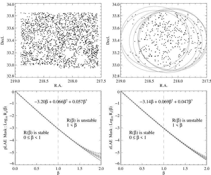
Figure A1.— The random sets for pLAE (top-left) and zLAE(top-right), and the corresponding RPFs, as defined in Equation 10, for pLAE (bottom-left) and for zLAE (bottom-right). For $0\leq\beta<1$, the self-consistent fit in Equation 11 is well defined mathematically.

Here, we describe the details about the divergence of Random Pair Functions (RPFs) and present their numerical forms, mentioned in §III.2.1. First, we recall the definition of RPF :

$$R_{\Omega}(\beta) \equiv \frac{\sum RR~{}\theta^{-\beta}}{\sum RR},$$ (A1)

where $RR$ is random pairs used for the LS estimator. From the definition, we can find two basic properties of RPF : (1) for a given $\beta$, RPF only depends on the random set, $RR$, and (2) for $\beta=0$, $R_{\Omega}(\beta=0)=1$. The first property indicates that RPF depends only on the geometric shape of survey volume, like the geometric form factor of the LS estimator. The second property guarantees that RPF is, at least, well-defined at $\beta=0$. For other $\beta$ values, it depends on the divergence of the integral sum, $\int_{0}^{\infty}\theta^{-\beta}d\theta$, whether RPF is well defined or not.

The integral sum of $\int_{0}^{\infty}\theta^{-\beta}d\theta$ is divided into three categories according to the values of $\beta$. For $0\leq\beta<1$, the tail sum of $\int_{1}^{\infty}\theta^{-\beta}d\theta$ diverges, while its local sum of $\int_{0}^{1}\theta^{-\beta}d\theta$ is finite. We refer to this as ``large scale divergence''. Conversely, for $1<\beta$, the local sum diverges, while the tail sum is finite. We refer to this as ``small scale divergence''. For $\beta=1$, the sum diverges logarithmically in both small and large scales. Generally, since observational surveys cover finite portions of sky, RPFs are well-defined functions for $0\leq\beta<1$; i.e., the sums in RPF are always finite real numbers.

Figure A1 shows the two random sets for pLAE and zLAE (top panels) and their corresponding RPFs (bottom panels). The grey cross points show the RPFs for 10 different random sets and we fit them, in the range of $0\leq\beta<1$, to obtain their numerical forms using cubic polynomials;

$$\log_{10}R_{p}(\beta) = -3.20\beta+0.066\beta^{2}+0.057\beta^{3}+O(\beta^{4})\textrm{ for pLAE},$$ (A2)

$$\log_{10}R_{z}(\beta) = -3.14\beta+0.069\beta^{2}+0.047\beta^{3}+O(\beta^{4})\textrm{ for zLAE.}$$ (A3)

The constant terms in Equation A2 and A3 are zero due to the boundary condition, $R_{\Omega}(\beta=0)=1$. We can find that the dominant terms are the first-order terms. The other higher order terms, $\beta^{2},\beta^{3},\cdots$, are minor and well truncated within $0\leq\beta<1$.

For $1<\beta$, the higher order terms, $\beta^{2},\beta^{3},\cdots$, are divergent, rather than truncated. And a small fraction of very close pairs (i.e., $\theta<<1$) dominates the total sum in RPF. Hence, the RPF values become very unstable (having extreme variance) for random sets due to the ``small scale divergence''. Therefore, the self-consistent fit in Equation 11,

$$\omega_{LS}(\theta) = \frac{\theta^{-\beta}-R_{\Omega}(\beta)}{A_{\omega}^{-1}+R_{\Omega}(\beta)},$$

is not valid for $1<\beta$. Fortunately, the fiducial value for $\beta$ in most practical cases is near 0.8; hence, within $0\leq\beta<1$. Equation 11 is, therefore, applicable in most cases.

Appendix B Physical Relevance vs. Statistical Interpretability in Parametric Models

In this section we discuss which halo occupation distribution (HOD) reliably represents the halo occupation of Boötes LAEs. We start with one of the most commonly used HODs,

$$N_{c}(M) = \left\{\begin{array}[]{ll}0&\textrm{if $M<M_{c}$},\\ 1&\textrm{if $M\geq M_{c}$},\end{array}\right.$$ (B3)

$$N_{s}(M) = \Big{(}\frac{M}{M_{1}}\Big{)}^{\alpha},$$ (B4)

where $N_{c}(M)$ represents central galaxy distribution and $N_{s}(M)$ satellite galaxy distribution for a given halo mass, $M$ (e.g., Zehavi et al. 2005; hereafter, we refer to this HOD as ZehaviHOD).

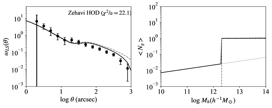
Figure B1.— The two point correlation functions (left) for observed LAEs (dots with error bars) and ZehaviHOD (lines; Zehavi et al. 2005), and halo occupation distribution (HODs; right) for ZehaviHOD. On the left panel, the dashed line represents the true two point function from the HOD Model without any effect of survey volume size, and the solid line the inversely corrected two point function using our inverse integral constraint method. On the right panel, the dashed line represents the average number of central galaxies, the dotted line of satellite galaxies, and the solid line of total galaxies. The HOD parameters for this model are $\log M_{1}=18.9$ and $\alpha=0.24$, selected from the posterior probability function, shown in Figure B2, with the estimates of $\log M_{1}=17.7^{+1.6}_{-1.6}$ and $\alpha=0.31^{+0.18}_{-0.08}$.

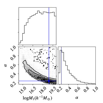
Figure B2.— The posterior probability function from the MCMC run for ZehaviHOD, visualized in contours (2D marginalized probabilities) and histograms (1D marginalized probabilities). We put 40 walkers (hence, 20 for each parameter) and run 700 steps. We discard the early 180 steps as burn-in and take 520 steps to retrieve the posterior probability function. The median values with $\pm 1\sigma$ errors for parameters are $\log M_{1}=17.7^{+1.6}_{-1.6}$ and $\alpha=0.31^{+0.18}_{-0.08}$. The (blue) lines and point represent the location of our parameter choice of $\log M_{1}=18.9$ and $\alpha=0.24$, where we demonstrate its two-point correlation function and HOD in Figure B1.

Figure B1 shows the two-point function (left) and HOD (right) for a ZehaviHOD, where we choose its model parameters from the posterior probability function shown in Figure B2, obtained using MCMC sampling. All results shown in Figure B1 and B2 are rough estimates, since the current outputs are already unlikely, $\log M_{1}=17.7^{+1.6}_{-1.6}$ and $\alpha=0.31^{+0.18}_{-0.08}$, indicating that ZehaviHOD is not physically relevant for describing emission line galaxies (ELGs). For example, the current ZehaviHOD predicts that the small halos with masses of $<10^{12}$ $M_{\odot}$ do not host LAEs at their centers; if any, they should be satellites. For massive halos, even if they host dust obscured galaxies at their centers, they should be detected in Ly$\alpha$ emission.

The duty cycle of LAEs is one of the main reasons why ZehaviHOD fails to be a relevant model. Unlike red dwarf stars serve as lifelong emission sources for galaxy, Ly$\alpha$ emission is only lit up for a short period of time. Hence, the halo occupation fraction should be allowed to be smaller than one. We write down a new HOD using duty cycles as,

$$N_{c}(M) = \left\{\begin{array}[]{ll}0&\textrm{if $M<M_{c}$},\\ F_{c}&\textrm{if $M\geq M_{c}$},\end{array}\right.$$ (B7)

$$N_{s}(M) = F_{s}\Big{(}\frac{M}{M_{1}}\Big{)}^{\alpha},$$ (B8)

where $F_{c}$ is a duty cycle for central LAEs and $F_{s}$ for satellite LAEs. By adding these two new parameters, we can achieve more physically relevant predictions to the halo occupation of LAEs. However, as a trade-off, we can lose statistical interpretability due to coupled parameters; moreover, there exists a potential degeneracy in model fits.

For example, the prediction of $\alpha\approx 0.3$ from ZehaviHOD is quite smaller than a fiducial value, $\alpha=1$. This is because the one-halo term is determined by center-satellite and satellite-satellite pair counts. Since the central occupation fraction is always equal to one for massive halos in ZehaviHOD, the number of satellites should be suppressed by taking unphysically high $\log M_{1}\approx 17$ and low $\alpha$ to match the observed small-scale clustering. If we take a small $F_{c}$, we can have a more parametric freedom to increase the number of satellites, while still fixing the total pair counts of center-satellite and satellite-satellite. Hence, by adding duty cycles to our new HOD, we can achieve more physically relevant predictions to $\log M_{1}$ and $\alpha$.

However, as a trade-off, we have a coupled factor, $F_{s}M_{1}^{-\alpha}$, for the satellite occupation in Equation B8. Though fixing this factor a constant, there are internal degenerate degrees of freedom among $\{F_{s},M_{1},\alpha\}$. In addition, $\{F_{c}\}$ is coupled with the satellite occupation parameters $\{F_{s},M_{1},\alpha\}$, which determines the number of center-satellite pairs, affecting small-scale clustering significantly.

Therefore, we can obtain a better HOD model by increasing its flexibility of functional form. However, we lose the model's interpretability due to explicit and implicit couplings among parameters and potentially the degeneracy increases in parameter estimates. If the duty cycle of LAEs is inevitably required for physical relevance, its related trade-offs are intrinsically ineluctable.

Before taking Equation B7 and B8 as our final HOD choice, we need to consider one more factor, the environmental effect on populating central LAEs. The question is whether it is physically relevant to populate the same fraction of LAEs at centers for different halos in various environments; for example, $10^{11}M_{\odot}$ halos mostly populated in field regions and $10^{13}M_{\odot}$ in dense regions. In a practical aspect, we need to decide whether it is necessary to add another set of parameters to the LAE's HOD for implementing such mass-dependent occupations. Unlike the duty cycle, this could be arguably optional for physical relevance, when considering the caveats of additional trade-offs caused by the new parameters.

For our sample, we have a conspicuous inflection point near 20″, which implies that the substructures of massive halos, determining the small-scale clustering, should be more accurately treated to properly explain the inflected feature. Therefore, we assign two different fractions of central occupations for the halos as,

$$N_{c}(M) = \left\{\begin{array}[]{ll}0&\textrm{if $M<M_{c}$},\\ F_{c}^{B}&\textrm{if $M_{c}\leq M\leq M_{\theta}$},\\ F_{c}^{A}&\textrm{if $M_{\theta}<M$},\end{array}\right.$$ (B12)

where $F_{c}^{A}$ and $F_{c}^{B}$ are central occupation fractions, split by a mass threshold $M_{\theta}$. Using this equation, we can assign different central occupations, for example, to $10^{11}M_{\odot}$ and $10^{13}M_{\odot}$ halos. As trade-offs, we have an explicit coupling among $\{F^{A}_{c},F^{B}_{c},M_{\theta}\}$ and an implicit dependence between $\{F^{A}_{c},F^{B}_{c},M_{\theta}\}$ and $\{F_{s},M_{1},\alpha\}$. Despite the issues of poor interpretability and potential degeneracy, we argue that the central occupations of LAEs for $10^{11}M_{\odot}$ and $10^{13}M_{\odot}$ halos should be different at $z\approx 2.67$. To conclude, by implementing the two physical factors of (1) duty cycles and (2) mass-dependent central occupations, our choice of physically relevant HOD for LAEs is Equation B8 and B12 with the 6 parameters $\{F_{c}^{A},F_{c}^{B},F_{s},M_{\theta},\alpha,M_{1}\}$.

In the literature, Geach et al. (2012) already implemented the two physical factors as,

$$N_{c}(M) = F_{c}^{B}(1-F_{c}^{A})\exp\Big{[}-\frac{\log(M/M_{c})^{2}}{2\sigma^{2}_{\log M}}\Big{]}$$ (B13)

$$+ F_{c}^{A}\Big{[}1+\textrm{erf}\Big{(}\frac{\log(M/M_{c})}{\sigma_{\log M}}\Big{)}\Big{]},$$

$$N_{s}(M) = F_{s}\Big{[}1+\textrm{erf}\Big{(}\frac{\log(M/M_{1})}{\delta_{\log M}}\Big{)}\Big{]}\Big{(}\frac{M}{M_{1}}\Big{)}^{\alpha}.$$ (B14)

where the main difference from Equation B8 and B12 is a smoother mass-dependence using Gaussian distribution with one additional parameter, $\delta_{\log M}$. When fixing $\delta_{\log M}\equiv 1$, the parameter set of Geach et al. is $\{F_{c}^{A},F_{c}^{B},F_{s},\sigma_{\log M},\alpha,M_{1}\}$, while $\{F_{c}^{A},F_{c}^{B},F_{s},M_{\theta},\alpha,M_{1}\}$ of Equation B8 and B12. Therefore, we adopt the HOD from Geach et al. for the Boötes LAEs for physical relevance considering the two factors of duty cycles and mass-dependent central occupations. Due to the inevitable trade-offs of poor interpretability and potential degeneracy, we accept all non-rejected HOD models as possible scenarios.

Appendix C Definitions of Network Quantities

All graph quantities presented in this section are commonly used in network science. Interested readers are referred to Newman (2003), Dorogovtsev, Goltsev & Mendes (2008), and Barthélemy (2011) for further details.

The Average Clustering Coefficient (average CC) is an average of all local clustering coefficients. The local clustering coefficient $C_{i}$ for a vertex $i$ is defined as,

$$C_{i} = \frac{\textrm{number of pairs of neighbors for }i~{}\textrm{that are connected}}{\textrm{number of pairs of neighbors for }i}.$$ (C1)

In social networks, the local clustering coefficient measures whether an individual s two friends know each other. The denominator in Equation C1 is the number of total pair combinations of the individual's friends. The numerator is the number of friended pairs; hence, triangular friendships when including the central individual. The local clustering coefficient, therefore, is roughly a triangle density for each vertex. The average of this vertex-wise triangle density is the average CC for a network.

Transitivity is a different version of triangle density from the average CC, defined as:

Transitivity $$= \frac{3\times\textrm{number of triangles}}{\textrm{number of connected triples}}.$$ (C2)

The top graph schema in Figure C1 illustrates the meaning of transitivity. The ``$\vee$'' configuration, connected by solid lines, is a connected triple. Transitivity is the fraction of whether the other side, drawn by a dotted line, is connected or not. Since a triangle contains three connected triples, transitivity is normalized to 1 as the average CC. Transitivity is often referred to as global clustering coefficient, since Equation C2 is a network-wise measurement while Equation C1 a vertex-wise measurement. Hence, we need to measure transitivity for a true unbiased triangle density for a network. The average CC is biased to the majority's CC value in vertex population due to the averaging process. Therefore, transitivity and average CC are similar, but not exactly the same.

A clique is a complete subgraph. Figure C2 show cliques with 3,4, and 5 vertices; hereafter, we refer to a clique with $k$ vertices as k-clique. Inside of the 5-clique, we can find many 3- and 4-subcliques. Generally, we can extend a clique by adding neighbors, until there is no more extendable clique configuration. This kind of un-extendable clique is referred to as maximal clique. Since galaxy groups and clusters form cliques in galaxy FOF networks, statistics of maximal cliques are quite interesting and important information for investigating the formation and evolution of galaxy groups and clusters. We find the largest maximal clique and measure its size from each network.

The Diameter is the largest path length of shortest pathways from all pairs in a network. The path length is defined as the number of steps to reach from a certain vertex, $i$, to another, $j$. Hence, the pathways of minimum path length are the shortest pathways between the vertices, $i$ and $j$; generally, there can be multiple shortest pathways between a pair in an unweighted network. The bottom graph schema in Figure C1 illustrates the shortest pathways between $i$ and $j$ vertices. There are three shortest pathways with the path length of 3. And there is one detour with the path length of 5. Therefore, the shortest path length between $i$ and $j$ is 3. We measure these shortest path lengths for all possible pairs in a network and, then, take the maximum value. This largest path length is defined as the diameter of the network.

Centrality is a value assigned to each vertex, as an indicator for quantifying which vertex is more important in a certain topological perspective. For example, Degree Centrality is the number of neighbors for each vertex. In social networks, this is a measure of the importance of a given individual in the network; the most influential individual is the one with the most ``friends", i.e., the one with the highest degree value. A better centrality can be defined if the current centrality cannot reflect the concerned topological feature well. The Google's PageRank is designed to prioritize the importance of World-Wide Web (WWW) documents. This centrality works better to rank WWW documents than the simple degree centrality (Page et al. 1999).

The Betweenness Centrality is a measure of which vertex is most frequently used when commuting back and forth between all pairs; hence, the congested spots during rush hours have high betweenness centralities in a road network. Mathematically, this betweenness, $x_{i}$ for the $i$-th vertex, is defined as:

$$x_{i}=\sum\limits_{st}\frac{n^{i}_{st}}{g_{st}},$$ (C3)

where $g_{st}$ is the number of shortest paths between the vertices $s$ and $t$, and $n^{i}_{st}$ the number of these which pass through the vertex, $i$. If $g_{st}$ is zero, we assign $n^{i}_{st}/g_{st}=0$. In the bottom graph schema of Figure C1, there are 3 shortest pathways between $i$ and $j$. By the definition of betweenness in Equation C3, we add $+1/3$ to all vertices on each shortest pathway. Then, $+2/3$ is assigned to red vertices and $+1/3$ is assigned to blue vertices by the pair of $i$ and $j$. We cumulate all of these betweenness values from all pairs to obtain the final betweenness centrality. Generally, this betweenness can be used to identify which spot is the most congested area in a road network or which person is the most influential broker connecting two isolated communities. In galaxy FOF networks, betweenness can be used as a filament tracer (Hong & Dey 2015).

Like the local clustering coefficient, betweenness and degree are vertex-wise measurements. As we average out local clustering coefficients to an average CC, we can measure the averages of betweenness and degree. However, for centralities, there is another way of reducing the vertex-wise values, referred to as centralization, which quantify how close a network is to a star graph, the most centralized graph structure. There are a couple of ways to define centralization. In this paper, we follow the Freeman's formula,

$$\textrm{Centralization}=\frac{\sum\limits_{i=1}^{n}[C_{max}-C_{i}]}{(n-1)(n-2)},$$ (C4)

where $C_{i}$ is a centrality value for a vertex $i$ and $C_{max}$ the maximum value of centrality. Figure  C3 shows Ring (left), Star (middle), and Clique (right) graphs with 7 vertices. The number on each vertex represents the number of neighbors (i.e., degree centrality), and the corresponding degree centralization and transitivity values are shown at the bottom of each graph. This demonstrates well how we can quantitatively discern the different kinds of network configurations using centralization and transitivity. In galaxy FOF networks, there is an interesting connection between star and clique that a star graph becomes a clique when we double the linking length from where a star graph forms. We refer to this as star–clique transition. If we find some anomaly in clique statistics, we may expect some related abnormal feature in centralization statistics at the half scale from where we find the clique anomaly.

The Giant component is the largest connected subgraph in a network. The giant components are trivial for the two extreme linking lengths in a galaxy FOF network. For a small linking length that isolates all individual galaxies, the size of the giant component is trivially 1. In the opposite case of a very large linking length forming a complete graph, the giant component size is equal to the total number of vertices (galaxies). Hence, the ratio of the size of giant component to the total number of vertices is a fraction that increases from 0 to 1 monotonically as the linking length grows from zero. This growth rate of giant component fraction depends on topology; especially aligned bridging structures like filaments, which connect vertices more efficiently than featureless random scatters. In this case, the fraction of giant component grows faster through the bridges to reach 1 at a smaller linking length than in the case of networks without such topological shortcuts.

Finally, the Edge Density is the number of edges divided by the total number of possible pairs, $n(n-1)/2$, to be normalized to 1.

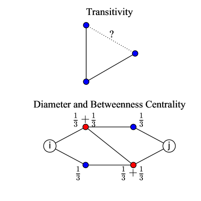
Figure C1.— The schematic figure illustrating the meanings of transitivity, diameter, and betweenness centrality.

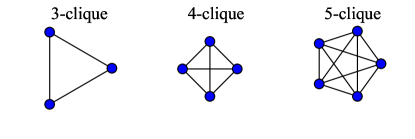
Figure C2.— A schematic figure showing 3, 4, and 5-cliques, where we refer to a complete subgraph with k–vertices as k–clique. Inside of the 5-clique, we can find many 3– and 4– subcliques. Generally, we can extend a clique by adding neighbors, until there is no more extendable clique configuration. This kind of un-extendable clique is referred to as maximal clique. Since galaxy groups and clusters form cliques in galaxy FOF networks, statistics of maximal cliques are quite interesting and important information for investigating the formation and evolution of galaxy groups and clusters.

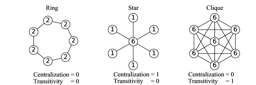
Figure C3.— A schematic figure showing Ring (left), Star (middle), and Clique (right) graphs with 7 vertices. The number on each vertex represents the number of neighbors (i.e., degree), and centralization and transitivity values are shown at the bottom for each graph. It is interesting that, in our FOF recipe for generating networks, a star graph becomes a clique when the linking length is doubled; hereafter, we refer to this as star–clique transition. Figures 10 and 11 provide some potential evidence of this star–clique transition.

References

- (1) Adelberger, K. L., et al. 2005, ApJ, 619, 697
- (2) Albert, R., & Barabási A.-L., 2002, Reviews of Modern Physics, 74, 47
- (3) Alon, N., Yuster, R., & Zwick, U. 1997, Algorithmica, 17, 209
- (4) Aragón-Calvo M. A., Jones B. J. T., van de Weygaert R., van der Hulst J. M., 2007, A&A, 474, 315
- (5) Aric A. Hagberg, Daniel A. Schult & Pieter J. Swart, Proceedings of the 7th Python in Science Conference (SciPy2008), Gäel Varoquaux, Travis Vaught, & Jarrod Millman (Eds), (Pasadena, CA USA), pp. 11 15, Aug 2008
- (6) Astropy Collaboration et al., 2013, A&A, 558, A33
- (7) Bardeen J. M., Steinhardt P. J. & Turner M. S., 1983, PRD, 28, 4, 679
- (8) Barkats, D. et al. 2014, ApJ, 783, 67
- (9) Barrow J. D., Bhavsar S. P., Sonoda D. H., 1985, MNRAS, 216, 17
- (10) Barthélemy, M. 2011, Physics Reports, 499, 1
- (11) Berlind, A. A., & Weinberg, D. H. 2002, ApJ, 575, 587
- (12) Bertin, E., & Arnouts, S. 1996, A&AS, 117, 393
- (13) Bond N. A., Strauss M. A., Cen R., 2010, MNRAS, 409, 156
- (14) Chiang, Y., Overzier, R., & Gebhardt, K. 2013, ApJ, 779, 127
- (15) Cole, S., et al. 2005, MNRAS, 362, 505
- (16) Cormen, T. H., et al. 2009, Introduction to Algorithms, 3rd Edition, The MIT Press, Cambridge, Massachusetts
- (17) Davis, M. & Peebles, P. J. E. 1983, ApJ, 26, 465
- (18) de Regt, R., et al. 2018, MNRAS, sty801
- (19) Dekel, A., & Birnboim, Y. 2006, MNRAS, 368, 2
- (20) Delubac, T., et al. 2015, A&A, 574, 59
- (21) Dorogovtsev, S. N., Goltsev, A. V., 2008, Rev. Mod. Phys., 80, 1275
- (22) Eisenstein D. J., Hu W. & Tegmark M., 1998, ApJ, 504, 57
- (23) Eisenstein D. J. et al., 2005, ApJ, 633, 560
- (24) Eisenbrand, F., & Grandoni, F. 2004, Theoretical Computer Science, 326, 57
- (25) Eriksen, H. K. et al. 2004, ApJ, 612, 64
- (26) Gawiser, E., et al. 2007, ApJ, 671, 278
- (27) Geach, J. E., et al. 2012, MNRAS, 426, 679
- (28) Genel, S., et al. 2014, MNRAS, 445, 175
- (29) Gil-Marin, H., et al. 2015, MNRAS, 451, 539
- (30) Gott J. R., Weinberg D. H., Melott A. L., 1987, ApJ, 319, 1
- (31) Guaita, L., et al. 2010, ApJ, 714, 255
- (32) Hill, G. J. et al. 2008, ASP Conf.Ser. 399, 115
- (33) Hinshaw, G. et al. 2013, ApJS, 208, 19
- (34) Huchra, J. P. & Geller, M. J. 1982, ApJ, 257, 423
- (35) James, G., Witten, D., Hastie, T., & Tibshirani, R., 2013, An introduction to statistical learning with applications in R. Springer.
- (36) Kereš, D., Katz, N., Weinberg, D. H., & Dave, R. 2005, MNRAS, 363, 2
- (37) Kereš, D., Katz, N., Fardal, M., Dave, R., & Weinberg, D. H. 2009, MNRAS, 395, 160
- (38) Kulkarni, G., et al. 2007, MNRAS, 378, 1196
- (39) Landy, S. D., & Szalay, A. S. 1993, ApJ, 412, 64
- (40) Lee, K. et al. 2014, ApJ, 796, 126
- (41) Levi, M. et al. 2013, arXiv:1308.0847
- (42) Mandelbrot, B. 1975, C. R. Acad. Sci. (Paris) A280, 1551
- (43) Martínez V. J., Starck J.-L., Saar E., Donoho D. L., Reynolds S. C., de la Cruz P., Paredes S., 2005, ApJ, 634, 744
- (44) More, S., et al. 2011, ApJS, 195, 4
- (45) Murray, S., Power, C., & Robotham, A. 2013, arXiv:1306.6721
- (46) Nelson, D., et al. 2015, A&C, 13, 12
- (47) Newman, M. E. J., 2003, SIAM Review, 45, 167
- (48) Newman, M. E. J., 2010, Networks: An Introduction. Oxford Univ. Press, Oxford
- (49) Orsi Á. A. et al. 2016, MNRAS, 456, 3827
- (50) Orsi Á. A. & Angulo R. E. 2017, arXiv:1708.00956
- (51) Ouchi, M., et al. 2010, ApJ, 723, 869
- (52) Planck Collaboration XVI 2014, A&A, 571, 16
- (53) Planck Collaboration XVII 2015, preprint (arXiv:1502.01592)
- (54) Planck CollaborationXI 2015, preprint (arXiv:1507.02704)
- (55) Pranav, P., et al. 2017, MNRAS, 465, 4281
- (56) Prescott, M. K. M., et al. 2008, ApJL, 678, 77
- (57) Seo H. J. & Eisenstein D. J., 2003, ApJ, 598, 2, 720
- (58) Starobinsky A. A., 1982, Phys. Lett. B, 117, 3-4, 175-178
- (59) Shandarin, S. F., & Zeldovich, Y. B., 1989, Reviews of Modern Physics, 61, 185
- (60) Sheth J. V., Sahni V., Shandarin S. F., Sathyaprakash B. S., 2003, MNRAS,343, 22
- (61) Soneira, R. M., & Peebles, P. J. E. 1978, AJ, 83, 845
- (62) Sousbie T., Pichon C., Courtois H., Colombi S., Novikov D., 2008, ApJ, 672, L1
- (63) Takahashi, R., et al. 2012, ApJ, 761, 152
- (64) Tinker, J. 2007, MNRAS, 374, 477
- (65) Tinker, J., et al. 2008, ApJ, 688, 709
- (66) van de Weygaert, R., et al. 2013, arXiv:1306.3640
- (67) Vogelsberger, M. 2014, Nature, 509, 177 (A)
- (68) Vogelsberger, M., et al. 2014, MNRAS, 444, 1518 (B)
- (69) Zhao, G, et al. 2015, arXiv:1510.08216
- (70) Zheng, Z., et al. 2005, ApJ, 633, 791