NIHAO XX: The impact of the star formation threshold on the cusp-core transformation of cold dark matter haloes

Abstract

We use cosmological hydrodynamical galaxy formation simulations from the NIHAO project to investigate the impact of the threshold for star formation on the response of the dark matter (DM) halo to baryonic processes. The fiducial NIHAO threshold, $n=10\,[{\rm cm}^{-3}]$, results in strong expansion of the DM halo in galaxies with stellar masses in the range $10^{7.5}\mathrel{\hbox to0.0pt{\lower 3.0pt\hbox{$\sim$}\hss}\raise 2.0pt\hbox{$<$}}{{M_{\rm star}}}\mathrel{\hbox to0.0pt{\lower 3.0pt\hbox{$\sim$}\hss}\raise 2.0pt\hbox{$<$}}10^{9.5}{{{\rm M}_{\odot}}}$. We find that lower thresholds such as $n=0.1$ (as employed by the EAGLE/APOSTLE and Illustris/AURIGA projects) do not result in significant halo expansion at any mass scale. Halo expansion driven by supernova feedback requires significant fluctuations in the local gas fraction on sub-dynamical times (i.e., $\mathrel{\hbox to0.0pt{\lower 3.0pt\hbox{$\sim$}\hss}\raise 2.0pt\hbox{$<$}}$ 50 Myr at galaxy half-light radii), which are themselves caused by variability in the star formation rate. At one per cent of the virial radius, simulations with $n=10$ have gas fractions of $\simeq 0.2$ and variations of $\simeq 0.1$, while $n=0.1$ simulations have order of magnitude lower gas fractions and hence do not expand the halo. The observed DM circular velocities of nearby dwarf galaxies are inconsistent with CDM simulations with $n=0.1$ and $n=1$, but in reasonable agreement with $n=10$. Star formation rates are more variable for higher $n$, lower galaxy masses, and when star formation is measured on shorter time scales. For example, simulations with $n=10$ have up to 0.4 dex higher scatter in specific star formation rates than simulations with $n=0.1$. Thus observationally constraining the sub-grid model for star formation, and hence the nature of DM, should be possible in the near future.

1 Introduction

The structure of dark matter haloes on kiloparsec-scales potentially provides the most sensitive astrophysical test of the cold dark matter (CDM) paradigm, and more generally the nature of dark matter (e.g., Bullock & Boylan-Kolchin, 2017). In dissipationless CDM simulations, the halo structure is well determined (e.g., Stadel et al., 2009; Dutton & Macciò, 2014). Gas dissipation is thought to only make the dark matter halo contract (Blumenthal et al., 1986; Gnedin et al., 2004). However, other baryonic processes can cause the dark matter halo to expand (e.g., El-Zant et al., 2001; Weinberg & Katz, 2002; Read & Gilmore, 2005; Pontzen & Governato, 2012). Due to the nonlinear nature of these processes and the importance of realistic initial conditions and evolution, their impact is best studied using cosmological hydrodynamical simulations.

Table 1: Simulation parameters. Box is the size of the parent DMO simulation. The halo ID corresponds to the virial mass of the parent DMO simulation. Number gives the number of haloes we run at a given resolution level, which is specified by the dark matter and gas particle masses, $m$, and gravitational force softenings, $\epsilon$.

Box	Halo ID range	Number	$m_{\rm gas}$	$\epsilon_{\rm gas}$	$m_{\rm DM}$	$\epsilon_{\rm DM}$
($h^{-1}$Mpc)	($h^{-1}$ M⊙)		(M⊙)	(pc)	(M⊙)	(pc)
60	g7.08e11 - g8.26e11	4	3.166$\times$105	397.9	1.735$\times$106	931.4
60	g1.37e11 - g3.71e11	8	3.958$\times$104	199.0	2.169$\times$105	465.7
60	g2.34e10 - g4.99e10	4	1.173$\times$104	132.6	6.426$\times$104	310.5
20	g7.05e09 - g1.23e10	4	3.475$\times$103	88.4	1.904$\times$104	207.0

Early simulations suffered from overcooling, forming an order of magnitude too many stars. The current generation of simulations is able to form galaxies with realistic amounts of stars and cold gas both today and in the past (Hopkins et al., 2014; Marinacci et al., 2014; Wang et al., 2015; Schaye et al., 2015). Improved numerical resolution has certainly helped, but the main difference is due to improved sub-grid models for star formation and feedback. Sub-grid models are necessary due to both the large dynamic range required to simulate cosmological scales and the formation of individual stars and the fact that the physics of star formation is still an unresolved problem. The sub-grid model attempts to capture the process by which gas turns into stars and the subsequent feedback of energy into the inter stellar medium (ISM) using effective models (i.e., averaged over many star formation and feedback events). Note that we do not necessarily need to understand how stars form on a micro level, but we do need an effective model of how stars form on kpc scales. Effective models are common in physics, for example, one can model atomic processes without an understanding of quarks.

Sub-grid models for star formation and feedback have several free parameters, which must currently be calibrated against observations (e.g., Schaye et al., 2015). In this paper we focus on a single parameter, the threshold for star formation, $n$. We choose this, because it is common among most sub-grid galaxy formation models, because it varies greatly $0.01\mathrel{\hbox to0.0pt{\lower 3.0pt\hbox{$\sim$}\hss}\raise 2.0pt\hbox{$<$}}n\mathrel{\hbox to0.0pt{\lower 3.0pt\hbox{$\sim$}\hss}\raise 2.0pt\hbox{$<$}}100\,[{\rm cm}^{-3}]$ in simulations with comparable numerical resolution, and because we have good reason to suspect it will influence how the dark halo responds to star formation (e.g., Pontzen & Governato, 2012). Furthermore, halo expansion is only seen in simulations that adopt a high threshold $n\mathrel{\hbox to0.0pt{\lower 3.0pt\hbox{$\sim$}\hss}\raise 2.0pt\hbox{$>$}}10$ (Governato et al., 2010; Macciò et al., 2012; Pontzen & Governato, 2012; Teyssier et al., 2013; Di Cintio et al., 2014a; Chan et al., 2015; Read et al., 2016; Tollet et al., 2016), while simulations with a low threshold $n\mathrel{\hbox to0.0pt{\lower 3.0pt\hbox{$\sim$}\hss}\raise 2.0pt\hbox{$<$}}0.1$ never find significant halo expansion (Oman et al., 2015; Schaller et al., 2015).

The goal of this paper is to test how the halo response depends on the threshold for star formation, and to determine any observational ways to distinguish between different thresholds. This paper is organized as follows. The simulation suite is outlined in section 2. Results for the stellar to halo masses and dark matter density profiles are shown in section 3. Section 4 gives a comparison between simulated and observed dark matter circular velocity profiles. Section 5 discusses the physical mechanism that drives the differences in halo response in our simulations and observational tests. A summary is given in section 6.

2 Simulations

We use a set of 20 haloes of virial masses between $\sim 10^{10}$ to $\sim 10^{12}{{{\rm M}_{\odot}}}$ drawn from the NIHAO project (Wang et al., 2015), and re-simulate them with three different $n$. Here we give a brief overview of the NIHAO simulations and we refer the reader to Wang et al. (2015) for a more complete discussion.

NIHAO is a sample of $\sim$ 100 hydrodynamical cosmological zoom-in simulations using the SPH code gasoline2 (Wadsley et al., 2017). Haloes are selected at redshift $z=0.0$ from parent dissipationless simulations of box size 60, 20, and 15 $h^{-1}$Mpc, presented in Dutton & Macciò (2014), which adopt a flat $\Lambda$CDM cosmology with parameters from the Planck Collaboration et al. (2014): Hubble parameter $H_{0}$= 67.1 ${\rm km\,s^{-1}}$ Mpc^-1; matter density $\Omega_{\rm m}=0.3175$; dark energy density $\Omega_{\rm\Lambda}=1-\Omega_{\rm m}=0.6825$; baryon density $\Omega_{\rm b}=0.0490$; power spectrum normalization $\sigma_{8}=0.8344$, and power spectrum slope $n=0.9624$. The corresponding cosmic baryon fraction ${f_{\rm bar}}\equiv\Omega_{\rm b}/\Omega_{\rm m}=0.154$. Haloes are selected uniformly in log halo mass from $\sim 10$ to $\sim 12$ without reference to the halo merger history, concentration or spin parameter.

2.1 Resolution

Dark matter particle masses and force softenings are chosen to resolve the mass profile at $\mathrel{\hbox to0.0pt{\lower 3.0pt\hbox{$\sim$}\hss}\raise 2.0pt\hbox{$<$}}1$ per cent of the virial radius according to the Power et al. (2003) criteria. This choice results in the dark matter profile being converged at $\simeq 2$ softening lengths and $\sim 10^{6}$ dark matter particles inside the virial radius of all main haloes at $z=0$. The corresponding gas particle masses and force softenings are a factor of $\Omega_{\rm b}/\Omega_{\rm dm}=0.182$ and $\sqrt{\Omega_{\rm b}/\Omega_{\rm dm}}=0.427$ lower. The particle masses and force softenings are given in Table. 1. Each hydro simulation has a corresponding dark matter only (DMO) simulation of the same resolution. These simulations have been started using the identical initial conditions, replacing baryonic particles with dark matter particles.

The simulations employ adaptive time steps. We start with 1024 major time steps each of 13.5 million years (Age of universe/1024), then the code refines this time step according to the acceleration of a particle. We allow for a maximum of 20 refinements which sets the minimum to 12.9 years (maximum time step/$2^{20}$).

2.2 Star formation

Star formation is implemented as described in Stinson et al. (2006, 2013). Stars form from cool ($T<15000$K), dense gas ($\rho>n$[cm^-3]). Gas eligible to form stars is converted into stars according to

$$\frac{\Delta{{M_{\rm star}}}}{\Delta t}=c_{\ast}\frac{M_{\rm gas}}{t_{\rm dyn}}.$$ (1)

Here $\Delta{{M_{\rm star}}}$ is the mass of stars formed, $\Delta t=0.84\,$Myr is the time-step between star formation events, and $t_{\rm dyn}$ is the gas particle’s dynamical time. The efficiency of star formation is set to $c_{\ast}=0.10$ for all simulations.

The main parameter of relevance to our study is the star formation threshold, $n$. In our fiducial NIHAO simulations we adopt $n=10[{\rm cm}^{-3}]\simeq 50m_{\rm gas}/\epsilon_{\rm gas}^{3}$. Here 50 is the number of particles used in the SPH smoothing kernel, $m_{\rm gas}$ is the initial mass of gas particles, and $\epsilon_{\rm gas}$ is the gravitational force softening of the gas particle. In our simulations we choose $\epsilon_{\rm gas}\propto m_{\rm gas}^{1/3}$, so that the star formation threshold is independent of the gas particle mass. We run each simulation at two additional star formation thresholds: $n=0.1$ and $n=1.0$. The former is similar to that adopted by the EAGLE/APOSTLE (Schaye et al., 2015; Sawala et al., 2016) and Illustris/AURIGA (Vogelsberger et al., 2014; Grand et al., 2017) projects. The FIRE project (Hopkins et al., 2014, 2018) uses star formation thresholds as high as $n=100$ or $n=1000$. We do not run simulations with such high values because our choice of gas mass and force softening do not enable us to resolve these densities. All simulations in the NIHAO project including the ones used here employ a pressure floor to keep the Jeans mass of the gas resolved and suppress artificial fragmentation.

Note that all of the thresholds we try are well below the density where stars form in the real Universe. Stars form in the cores of giant molecular clouds at densities of $\rho\sim 10^{4}\,[{\rm cm}^{-3}]$. Giant molecular clouds have typical densities of $\rho\sim 100\,[{\rm cm}^{-3}]$, while molecular gas typically forms at densities $\rho\mathrel{\hbox to0.0pt{\lower 3.0pt\hbox{$\sim$}\hss}\raise 2.0pt\hbox{$>$}}10\,[{\rm cm}^{-3}]$. Thus it might be surprising if star formation could be modeled accurately on kpc scales using a density threshold as low as $n=0.1$. However, as discussed in the introduction, we are not modeling individual star formation and SN events, but rather an ensemble of them. So it might be possible to capture the essential features of star formation and feedback using an effective star formation threshold that is much lower than that for individual star forming regions.

2.3 Feedback

The NIHAO simulations employ thermal feedback in two epochs following Stinson et al. (2013). In the first epoch, ‘pre-SN feedback’ (early stellar feedback, ESF) happens before any supernovae explode. The ESF represents stellar winds and photoionization from the bright young stars. The ESF consists of a fraction $\epsilon_{\rm ESF}$ of the total stellar flux being ejected from stars into surrounding gas ($2\times 10^{50}$ erg of thermal energy per ${{{\rm M}_{\odot}}}$ of the entire stellar population). Radiative cooling is left on for the pre-SN feedback. The second epoch starts 4 Myr after the star forms, when the first supernovae start exploding. Only supernova energy is considered as feedback in this second epoch. Stars with mass $8\,{{{\rm M}_{\odot}}}<M_{\ast}<40\,{{{\rm M}_{\odot}}}$ eject both energy ($\epsilon_{\rm SN}\times 10^{51}$ erg/SN) and metals into the interstellar medium gas surrounding the region where they formed. Supernova feedback is implemented using the blastwave formalism described in Stinson et al. (2006). Since the gas receiving the energy is dense, it would be quickly radiated away due to its efficient cooling. For this reason, cooling is delayed for particles inside the blast region for $\sim 30$ Myr. The free parameters of the feedback model $\epsilon_{\rm ESF}=0.13,\epsilon_{\rm SN}=1.0$ were calibrated against the evolution of the stellar mass versus halo mass relation from halo abundance matching (Behroozi et al., 2013; Moster et al., 2013) for a $z=0$ Milky Way mass halo $\sim 10^{12}{{{\rm M}_{\odot}}}$.

In EAGLE, energy feedback from star formation is implemented using the stochastic thermal prescription of Dalla Vecchia & Schaye (2012). Rather than delay cooling, they delay the injection of energy into gas particles so that those particles that get heated are too hot to cool efficiently. The energy injected per unit stellar mass formed decreases with the metallicity of the gas and increases with the gas density to account for unresolved radiative losses and to help prevent spurious numerical losses. The free parameters of the EAGLE star formation and feedback model are calibrated against the observed, $z=0$ galaxy stellar mass function and the size versus stellar mass relation of $z\simeq 0$ star-forming galaxies (Crain et al., 2015).

In NIHAO and EAGLE galactic winds develop naturally, without imposing mass loading factors, velocities or directions. On the other hand, the AURIGA simulations adopt a kinetic feedback model in which gas particles isotropically surrounding a star particle are given a kick with velocity proportional to the 1D velocity dispersion of the surrounding dark matter particles and a mass loading factor of 0.6. All three models described above are obviously approximations of how feedback actually occurs, yet they are successful in that they form galaxies with realistic stellar masses and sizes.

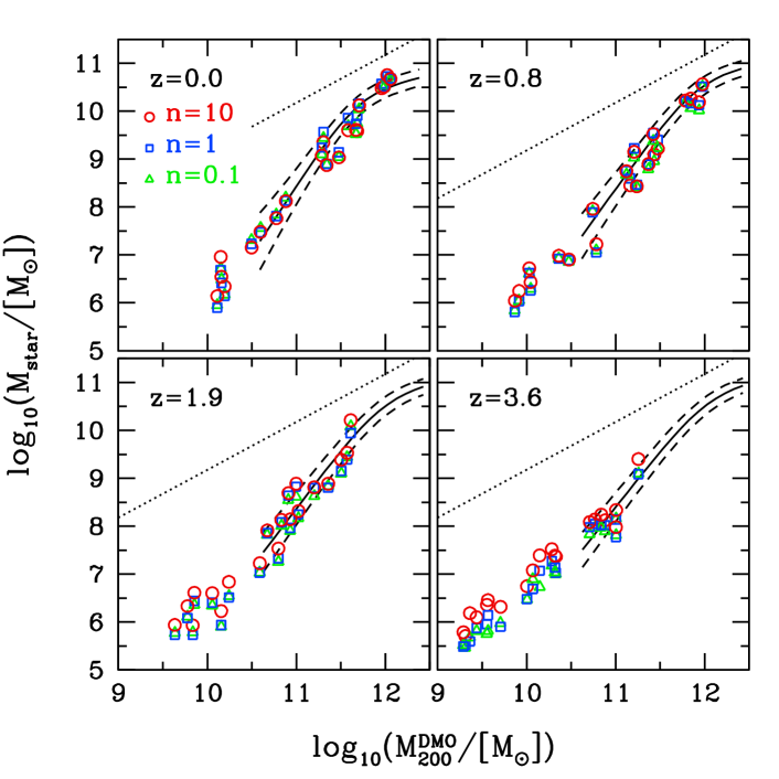
Figure 1: Stellar mass of hydro simulation versus virial mass of DMO simulation at four redshifts. Simulations with different star formation thresholds ($n$) are shown with different colours and symbols: $n=10$ (red circles), $n=1$ (blue squares), $n=0.1$ (green triangles). We compare to the abundance matching relations from Moster et al. (2018) (mean and scatter). The dotted line shows the cosmic baryon fraction.

2.4 Haloes and galaxies

Haloes are identified using the MPI+OpenMP hybrid halo finder AHF (Gill et al., 2004; Knollmann & Knebe, 2009). AHF locates local over-densities in an adaptively smoothed density field as prospective halo centers. The virial masses of the haloes are defined as the masses within a sphere whose average density is 200 times the cosmic critical matter density, $\rho_{\rm crit}=3H_{0}^{2}/8\pi G$. The virial mass, size and circular velocity of the hydro simulations are denoted: $M_{200}$, $R_{200}$, $V_{200}$. The corresponding properties for the DMO simulations are denoted with a superscript, ${\rm DMO}$. For the baryons, we calculate masses enclosed within spheres of radius $r_{\rm gal}=0.2R_{200}$, which corresponds to $\sim 10$ to $\sim 50$ kpc. The stellar mass inside $r_{\rm gal}$ is $M_{\rm star}$, the neutral hydrogen, Hi, inside $r_{\rm gal}$ is computed following Rahmati et al. (2013) as described in Gutcke et al. (2017).

The NIHAO simulations are the largest set of cosmological zoom-ins covering the halo mass range $10^{10}$ to $10^{12}{{{\rm M}_{\odot}}}$. Their uniqueness is in the combination of high spatial resolution coupled to a statistical sample of haloes. As discussed in previous papers in the NIHAO series, NIHAO galaxies are consistent with a wide range of galaxy properties in both the local and distant Universe. In the context of $\Lambda$CDM, they form “right” amount of stars both today and at earlier times (Wang et al., 2015). Their cold gas masses and sizes are consistent with observations (Stinson et al., 2015; Macciò et al., 2016; Dutton et al., 2019), they follow the gas, stellar, and baryonic Tully-Fisher relations (Dutton et al., 2017). They match the observed clumpy morphology of galaxies seen at high redshifts (Buck et al., 2017). On the scale of dwarf galaxies the dark matter haloes expand yielding cored dark matter density profiles consistent with observations (Tollet et al., 2016), and resolve the too-big-to-fail problem of field galaxies (Dutton et al., 2016a). They reproduce the diversity of dwarf galaxy rotation curve shapes Santos-Santos et al. (2018), and the Hi linewidth velocity function (Macciò et al., 2016; Dutton et al., 2019). As such they are a good template with which to predict the structure of cold dark matter haloes.

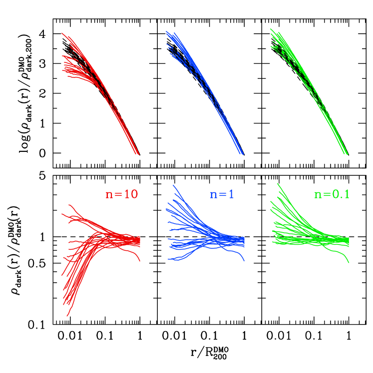
Figure 2: Enclosed dark matter density profiles, where $\rho(r)=M(<r)/(4/3\pi r^{3})$. Dashed lines show DMO simulation scaled by $(1-{f_{\rm bar}})=0.85$, solid lines show dark matter density profiles from the hydrodynamical simulations with $n=10$ (red, left), $n=1$ (blue, middle), and $n=0.1$ (green, right). Lines are plotted from twice the dark matter softening ($\approx$ convergence radius) to the virial radius.

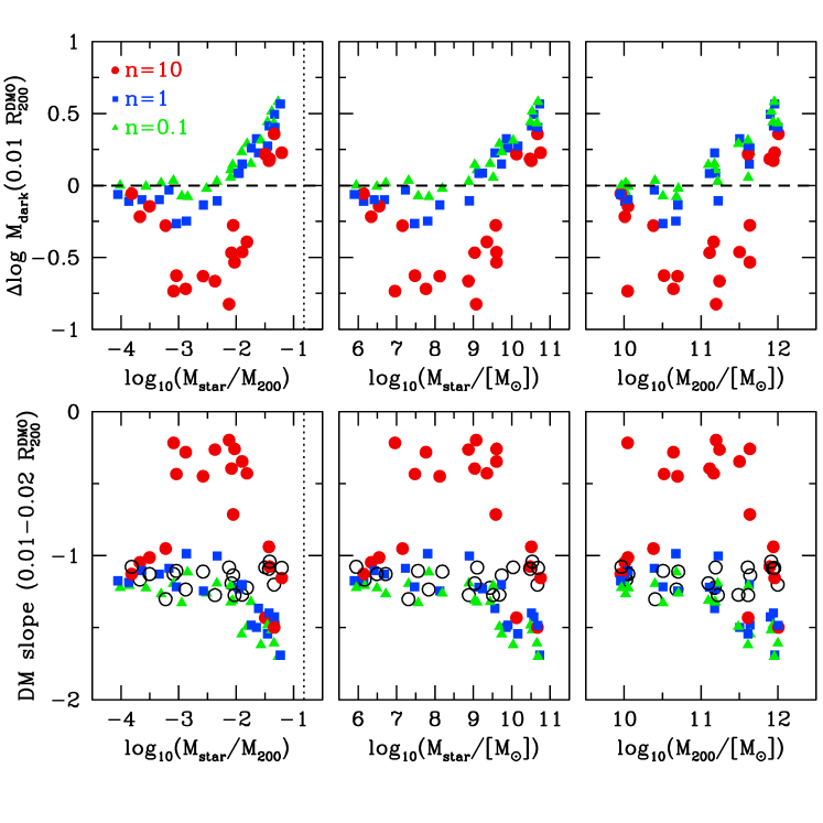
Figure 3: Change in enclosed mass ($\Delta\log M_{\rm dark}\equiv\log M_{\rm dark}-\log M_{\rm dark}^{\rm DMO}$) at 1 per cent of the virial radius (upper panels) and slope of the enclosed dark matter density profile between 1 and 2 per cent of the virial radius (lower panels) versus halo mass (right), stellar mass (middle), and stellar to halo mass ratio (left). The dotted line in the left panels corresponds to the cosmic baryon fraction.

3 Results

3.1 Stellar to halo mass

We start our discussion of the simulations with the two most basic properties: the total mass within the virial radius of the DMO simulation $M_{200}^{\rm DMO}$; and the stellar mass (within 20 per cent of the virial radius) of the corresponding hydrodynamical simulation, ${{M_{\rm star}}}$. Fig. 1 shows the stellar versus halo mass relation for the main halo in each of our simulations at four redshifts: $z=3.6$, $z=1.9$, $z=0.8$, and $z=0.0$.

The different symbols show the three star formation thresholds: $n=10$ (red circles), $n=1$ (blue squares), $n=0.1$ (green triangles). We maintain this colour and symbol scheme throughout the paper. Simulations with $n=10$ and $n=1$ have sufficiently similar stellar masses that we do not re-calibrate the feedback efficiency. However, for the $n=0.1$ simulations the stellar masses are significantly lower by redshift $z=0$: a factor of $\sim 2$ for $M_{200}\sim 10^{10}{{{\rm M}_{\odot}}}$, and a factor of $\sim 8$ for $M_{200}\sim 10^{12}{{{\rm M}_{\odot}}}$. For simplicity we adjust one of the feedback parameters, $e_{\rm ESF}$, the fraction of the energy from young stars that couples to the ISM. The fiducial simulations have $e_{\rm ESF}=0.13$, which we reduce to $e_{\rm ESF}=0.04$ for the $n=0.1$ simulations, such that the $z=0$ stellar masses are nearly equal to the corresponding masses in the $n=1$ and $n=10$ cases. This re-calibration is an important step that is often not taken. It enables us to compare the halo responses of the different thresholds, without having to worry about other processes. For example, Governato et al. (2010) simulate a single halo with $n=100$ and $n=0.1$. The $n=100$ halo expands, while the $n=0.1$ halo contracts. However, the low threshold simulation formed an order of magnitude more stars, so it is hard to disentangle the effects of increased dissipation with the effects of a low threshold.

The dotted lines show the maximum stellar mass, corresponding to all of the cosmically available baryons turning into stars. The solid and dashed lines show the mean and $1\sigma$ scatter relations from halo abundance matching (Moster et al., 2018). Here we have converted the halo masses of the relations to our definition, $M_{200}/(4/3\pi R_{200}^{3})=200\rho_{\rm crit}$, using the concentration mass relations from Dutton & Macciò (2014). We have interpolated the fitting coefficients from Moster et al. (2018) to the redshifts that we show. Fig. 1 shows that our simulations with different star formation thresholds form the “correct” (in the context of $\Lambda$CDM) amount of stars both today and at earlier cosmic times.

3.2 Density profiles

Fig. 2 shows the enclosed dark matter density profiles, $\rho(r)\equiv 3M(<r)/(4\pi r^{3})$, for the simulations at $z=0$. We use enclosed rather than local dark matter density profiles because the former are more robust being independent of binning. Coloured lines correspond to the hydro simulations. Black dashed lines show the DMO simulations with a rescaling of the total density profile by $1-{f_{\rm bar}}\simeq 0.85$. The re-scaling is done so that when we compare profiles from hydro and DMO simulations, a ratio of unity corresponds to no halo response. Upper panels show the density profiles and lower panels show the ratio with respect to the DMO simulation. Lines which are above unity thus correspond to halo contraction, while lines below unity correspond to halo expansion. All thresholds result in the same behaviour at large radii, namely a small amount of (adiabatic) halo expansion due to the loss of baryons from the halo. The exception is halo g2.19e11, which has a higher halo mass in DMO due to a major merger that has been delayed in the hydro simulations.

Below 10 per cent of the virial radius the simulation results start to diverge, both in the magnitude of the expansion and contraction. The $n=0.1$ simulations show a variation of a factor of $\simeq 5$ with respect to the DMO simulations, the $n=1$ simulations a factor of $\simeq 6$, and the $n=10$ simulations a factor of $\sim 10$. Thus for all of the star formation thresholds we try, the cold dark matter haloes are not described by a universal function, as is the case for DMO simulations.

The diversity in halo response at small radii is more clearly shown in Fig. 3. Upper panels show the change in the dark matter mass profile at 1 per cent of the virial radius (identical to the change in enclosed dark matter density), while lower panels show the slope of the enclosed dark matter density profile between 1 and 2 per cent of the virial radius. Note that here we use the enclosed dark matter density rather than the local dark matter density as used in our previous works (e.g., Tollet et al., 2016), but the results are qualitatively the same.

In the upper panels, the dashed line corresponds to the DMO simulation (by definition), while in the lower panels the open circles show the DMO simulations. Results are shown versus halo mass (right), stellar mass (middle), and stellar-to-halo mass ratio (left). The latter has been shown to be better correlated with the halo response (Di Cintio et al., 2014a; Dutton et al., 2016b; Bullock & Boylan-Kolchin, 2017) in simulations with high star formation thresholds, than either the stellar mass or halo mass alone.

At the lowest ${{M_{\rm star}}}/M_{200}\sim 10^{-4}$ all of the simulations result in no significant changes to the density profile. At higher efficiencies of $10^{-3}$ to $10^{-2}$, the $n=0.1$ simulations still have no significant change, but the $n=1$ simulations have a small amount of expansion, while the $n=10$ simulations have a large amount of expansion. At ${{M_{\rm star}}}/M_{200}>10^{-2}$, the $n=0.1$ and $n=1$ simulations result in halo contraction, which strengthens for higher efficiencies. At the highest ${{M_{\rm star}}}/M_{200}$, the $n=10$ simulations also contract, but not as strongly as the lower $n$ simulations.

We note that our results for $n=0.1$ are very similar to those for the APOSTLE and AURIGA simulations recently presented by Bose et al. (2018). This is in spite of numerous differences between the codes, including how supernova feedback is modeled and the hydrodynamical schemes. This strengthens the notion that the star formation threshold is the key sub-grid parameter that controls the halo response in haloes of mass $M_{200}\mathrel{\hbox to0.0pt{\lower 3.0pt\hbox{$\sim$}\hss}\raise 2.0pt\hbox{$<$}}10^{12}{{{\rm M}_{\odot}}}$.

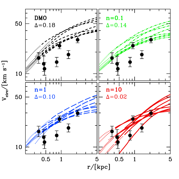
Figure 4: Circular velocity versus radius. Lines show simulations with stellar masses $10^{6}\mathrel{\hbox to0.0pt{\lower 3.0pt\hbox{$\sim$}\hss}\raise 2.0pt\hbox{$<$}}{{M_{\rm star}}}\mathrel{\hbox to0.0pt{\lower 3.0pt\hbox{$\sim$}\hss}\raise 2.0pt\hbox{$<$}}10^{8}{{{\rm M}_{\odot}}}$. The transition from dotted to solid/dashed lines marks the scale that is accurately resolved (twice the dark matter softening). Points with error bars show observed field galaxies more than 500 kpc from the Milky Way (Kirby et al., 2014). The parameter $\Delta$ is the mean offset between the observations and the simulations. The DMO simulations (upper left) are offset from the observations by an average of 0.18 dex (i.e., a factor of 1.5). As the star formation threshold increases the offset decreases, such that with $n=10$ (lower right) the offset is just 0.02 dex. This shows that different star formation thresholds result in testable differences in the structure of cold dark matter haloes.

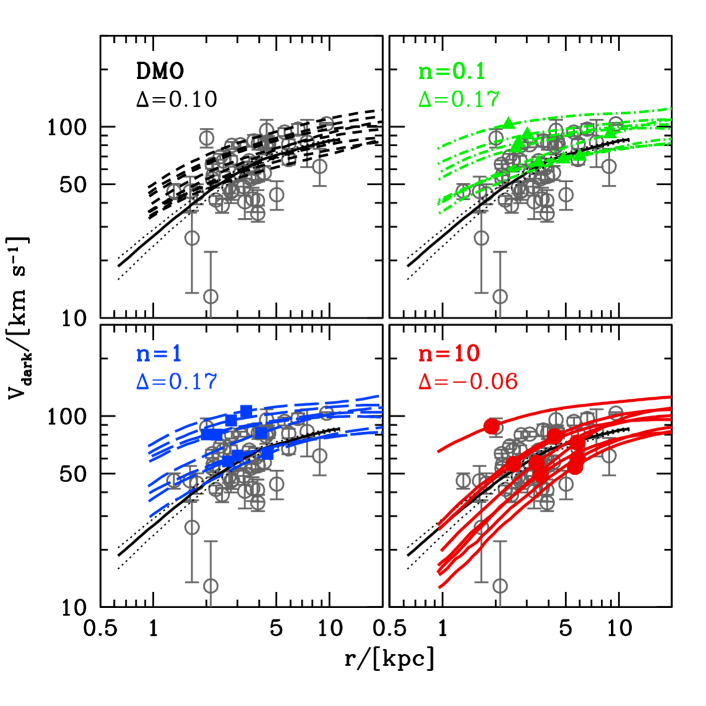
Figure 5: Dark matter circular velocity versus radius for galaxies with $10^{9}\mathrel{\hbox to0.0pt{\lower 3.0pt\hbox{$\sim$}\hss}\raise 2.0pt\hbox{$<$}}{{M_{\rm star}}}\mathrel{\hbox to0.0pt{\lower 3.0pt\hbox{$\sim$}\hss}\raise 2.0pt\hbox{$<$}}10^{10}{{{\rm M}_{\odot}}}$. The same observations are shown in all panels. Grey circles with error-bars show the dark matter circular velocity within the half-light radius for observed galaxies from SPARC. The solid black line shows the mean dark matter circular velocity curve of the observations, while the dotted lines show the impact of a 0.1 dex uncertainty in stellar mass-to-light ratio. Each panel shows a different set of simulations: DMO (upper left, black); $n=0.1$ (upper right, green); $n=1.0$ (lower left, blue); and $n=10$ (lower right, red). The points correspond to the half stellar mass radii . The value $\Delta$ is the mean offset [dex] between the simulations and the observed dark matter velocity at 2 kpc.

4 Velocity profiles

We now discuss the circular velocity profiles of the simulations to highlight the magnitude of the observational differences one can expect. We split the simulations into three mass ranges corresponding to dwarf galaxies ($10^{6}\mathrel{\hbox to0.0pt{\lower 3.0pt\hbox{$\sim$}\hss}\raise 2.0pt\hbox{$<$}}{{M_{\rm star}}}/{{{\rm M}_{\odot}}}\mathrel{\hbox to0.0pt{\lower 3.0pt\hbox{$\sim$}\hss}\raise 2.0pt\hbox{$<$}}10^{8}$), intermediate mass galaxies ($10^{9}\mathrel{\hbox to0.0pt{\lower 3.0pt\hbox{$\sim$}\hss}\raise 2.0pt\hbox{$<$}}{{M_{\rm star}}}/{{{\rm M}_{\odot}}}\mathrel{\hbox to0.0pt{\lower 3.0pt\hbox{$\sim$}\hss}\raise 2.0pt\hbox{$<$}}10^{10}$), and Milky Way mass galaxies (${{M_{\rm star}}}\sim 5\times 10^{10}{{{\rm M}_{\odot}}}$).

4.1 Dwarf galaxies

We start with the 8 lowest mass haloes which form galaxies of stellar masses $10^{6}\mathrel{\hbox to0.0pt{\lower 3.0pt\hbox{$\sim$}\hss}\raise 2.0pt\hbox{$<$}}{{M_{\rm star}}}\mathrel{\hbox to0.0pt{\lower 3.0pt\hbox{$\sim$}\hss}\raise 2.0pt\hbox{$<$}}10^{8}{{{\rm M}_{\odot}}}$. Fig. 4 shows the circular velocity profiles (lines) of these simulations compared to the circular velocity at the 3D half-light radius of field dwarf galaxies in the local group (points with error bars) from Kirby et al. (2014). We have selected observed dwarfs with V-band luminosities from $10^{6}$ to $2\times 10^{8}{{{\rm L}_{\odot}}}$ with distances of at least 500 kpc ($\sim 2$ virial radii) from the Milky Way to minimize contamination of back-splash galaxies (Buck et al., 2018).

Qualitatively, we see that the DMO simulations are systematically too high, while the $n=10$ simulations can match all of the observations. The lower threshold simulations ($n=0.1,n=1$) can reproduce some, but not all of the observed data points. To be more quantitative, we calculate the average offset between the observations ($V_{\rm obs}$) and simulations $V_{\rm sim}$. For each observed data point, $V_{{\rm obs},i}$, the mean offset with respect to the $N_{\rm sim}=8$ simulations is

$$\Delta_{i}=\sum_{j=1}^{N_{\rm sim}}(\log_{10}V_{{\rm obs},i}-\log_{10}V_{{\rm sim},j})/N_{\rm sim}.$$ (2)

We then take the mean of $\Delta_{i}$ over the 7 observed data points, which we denote $\Delta$. For DMO (upper left panel), $\Delta=0.18$, i.e. the average offset between simulation and observation is a factor of 1.5 in velocity, and a factor of 2.3 in enclosed mass. This recovers the well known Too-big-to-fail (TBTF) problem of local group field galaxies (Garrison-Kimmel et al., 2014). We showed previously in Dutton et al. (2016a) that the NIHAO simulations resolve this problem. Indeed for the fiducial NIHAO $n=10$ (lower right), the simulations match the observations well with $\Delta=0.02$. However, the hydro simulations with lower thresholds predict less halo expansion and tend to over-predict the observations. The $n=1$ simulations have $\Delta=0.10$ (a factor of $1.25$ to high), and the $n=0.1$ simulations have $\Delta=0.14$ (a factor of $1.4$ to high).

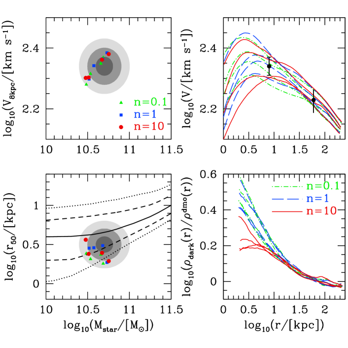
Figure 6: Results for Milky Way mass haloes. Left panels show the circular velocity at 8 kpc versus stellar mass (upper) and projected half stellar mass radius versus stellar mass (lower). Ellipses show the 1,2, and $3\sigma$ uncertainties for the Milky Way. For the sizes the lines show the median (solid), $1\sigma$ (dashed) and $2\sigma$ (dotted) relations for observations from SDSS. The upper right panel shows the total circular velocity versus radius. The points with error bars show observational constraints. The lower right panel shows the change in enclosed dark matter density profile between hydro and DMO simulations. In all panels the colour refers to the star formation threshold: $n=10$ (red), $n=1$ (blue), $n=0.1$ (green).

The current observations clearly favor CDM simulations with a high star formation threshold. Turning this around, if a low star formation threshold can be shown to be a better description for star formation in sub-grid models of galaxy formation, then this test can be used to falsify the CDM model. While this test is not conclusive due to the small number statistics of the observations, we can conclude that simulations with different star formation thresholds make clear testable differences in the circular velocities on scales of 1 kpc.

4.2 Intermediate mass galaxies

We next consider galaxies of stellar mass $10^{9}\mathrel{\hbox to0.0pt{\lower 3.0pt\hbox{$\sim$}\hss}\raise 2.0pt\hbox{$<$}}{{M_{\rm star}}}\mathrel{\hbox to0.0pt{\lower 3.0pt\hbox{$\sim$}\hss}\raise 2.0pt\hbox{$<$}}10^{10}{{{\rm M}_{\odot}}}$. There are 8 sets of simulations in this mass range. These simulations show a large disparity in the halo response with strong expansion for $n=10$ and no change or mild contraction for $n=0.1$ and $n=1$ (see Fig. 3).

We compare to galaxies from the SPARC survey of nearby star forming galaxies (Lelli et al., 2016). Fig. 5 shows the dark matter circular velocity profiles. For observations these are obtained by subtracting the stellar and gas circular velocity profiles from the total rotation velocity, assuming a stellar mass-to-light ratio at $3.6\,\mu$m of 0.5. For the observations the grey symbols show the dark matter velocity at the half-light radius. The solid black line shows the average dark matter velocity profile of the observations plotted between the average smallest and largest point on the rotation curve. Because these galaxies tend to be dark matter dominated, there is only a small uncertainty in the dark matter profile caused by the 0.1 dex uncertainty in stellar mass-to-light ratio (dotted lines).

For the NIHAO simulations, each panel shows a different simulation: DMO (top left), $n=0.1$ (top right), $n=1$ (bottom left), and $n=10$ (bottom right). The lines show the dark matter circular velocity profiles, where the DMO has been rescaled by the cosmic baryon fraction ($\sqrt{1-{f_{\rm bar}}}\simeq 0.92$). Symbols are located at the projected half-mass radius of the stars. This shows that the galaxy sizes for these simulations are in reasonable agreement with the observations and that there is only a small dependence of the sizes on the star formation threshold. Overall, every simulated galaxy has an observed counterpart within a small interval of radius and velocity. Going further, we can match the full circular velocity curves, or dark matter circular velocity curves, to find good observational analogs of all the simulated galaxies.

However, only the $n=10$ simulations can reproduce the full range of observed velocities in Fig. 5. The low thresholds are unable to significantly expand the dark matter halo. Qualitatively when comparing the simulated dark matter profiles to the observed mean, we see that the high threshold ($n=10$) simulations tend to be below the observed mean, while the low threshold simulations ($n=0.1,n=1$) tend to be above the mean relation. Being quantitative, the parameter $\Delta$ is the mean offset between the simulations and the observed dark matter velocity at 2 kpc. DMO has $\Delta=0.1$. The $n=0.1$ and $n=1$ simulations have higher $\Delta=0.17$, which indicates the haloes are contracting. The $n=10$ simulations have $\Delta=-0.06$ indicating expansion. Our sample of simulations is small, so the cosmic variance could be large. With that caveat aside, there are two generic solutions to resolve this discrepancy.

On the observational side there could be a systematic that biases the rotation curves low (or high), possibly from non-circular motions due to pressure support or triaxial dark matter haloes (Valenzuela et al., 2007; Oman et al., 2019). On the theoretical side, a threshold between 1 and 10 could possibly result in a better match to observations. More interesting is the possibility that a single star formation threshold is too simplistic and that a variable threshold captures better the physics of star formation at the resolution of our simulations. This variability could occur systematically with other properties of the gas, or it could be essentially a random variable at the scales we are considering. Indeed Semenov et al. (2017) present a model in which the threshold for star formation is a function of both the gas density, $n$, and the total subgrid velocity dispersion, $\sigma_{\rm tot}=\sqrt{c_{s}^{2}+\sigma_{\rm turb}^{2}}$, where $c_{s}$ is the sound speed, and $\sigma_{\rm turb}$ are the explicitly modeled sub-grid turbulent velocities. In this model the effective star formation threshold varies from $n\sim 10$ to $n\sim 1000$.

4.3 Milky Way mass galaxies

Fig. 6 shows results for the four most massive simulations. Top left shows circular velocity at 8 kpc versus stellar mass, bottom left shows projected half stellar mass radius versus stellar mass. Observational estimates for these values for the Milky Way are shown with ellipses corresponding to the 1,2,3 $\sigma$ uncertainty which are based on results from dynamical models of Widrow et al. (2008) and Bovy & Rix (2013).

• Circular Velocity. We adopt a circular velocity at 8 kpc (the solar radius) of $\log_{10}(V_{8\rm kpc}/[{{{\rm km\,s^{-1}}}}])=2.34\pm 0.03$, which gives a $2\sigma$ range from 191 to 251 ${{{\rm km\,s^{-1}}}}$.

• Stellar Mass. We adopt $\log_{10}(M_{\rm star}/[{{{\rm M}_{\odot}}}])=10.7\pm 0.1$, which gives a $2\sigma$ range from 3.2 to $7.9\times 10^{10}{{{\rm M}_{\odot}}}$. Widrow et al. (2008) finds a disk stellar mass of $4.22\pm 0.51\times 10^{10}{{{\rm M}_{\odot}}}$ and a bulge mass of $0.96\pm 0.12\times 10^{10}{{{\rm M}_{\odot}}}$. Bovy & Rix (2013) finds a disk stellar mass of $4.6\pm 0.3\times 10^{10}{{{\rm M}_{\odot}}}$.

• Half-Mass Size. We adopt $\log_{10}(r_{50}/[{\rm kpc}])=0.5\pm 0.1$, which gives a $2\sigma$ range from 2.0 to 5.0 ${\rm kpc}$. Widrow et al. (2008) finds a disk scale length of $R_{\rm d}=2.8\pm 0.23$ (their prior had limits 2.0 to 3.8 kpc), corresponding to a half-mass size of $r_{50}=4.7\pm 0.4$. Bovy & Rix (2013) finds a disk stellar mass scale length of $R_{\rm d}=2.15\pm 0.14$ kpc, corresponding to a half-mass size of $r_{50}=3.61\pm 0.23$. These disk sizes are likely an upper limit to the total half-light size once the central bulge is included. For example, if 20 per cent of the stellar mass is in a compact bulge (Widrow et al., 2008), then the half-mass radius of the galaxy is roughly 1.1 disk scale lengths. For the sizes the lines show observations from SDSS (Dutton et al., 2011; Simard et al., 2011) for various percentiles of the distribution of sizes in bins of stellar mass: median (solid), 15.9 and 84.1 (dashed), 2.3 and 97.7 (dotted). This shows that the Milky Way is about $1\sigma$ smaller (with a large uncertainty) than typical galaxies of the same stellar mass.

We see that the velocities, stellar masses, and sizes are not sensitive to the star formation threshold and that all 12 simulations fall within the observed $3\sigma$ ranges.

The top right panel shows the total circular velocity profile from 1 kpc to the virial radius. The circular velocity profile has two observational data points (black error bars): the velocity at 8 kpc (from above), and the velocity at 60 kpc (Xue et al., 2008). All simulations are consistent with these observational constraints. The bottom right panel shows the change in the dark matter density profile with respect to DMO. We see similarities and differences in halo response between simulations with different star formation thresholds.

Similarities: At large radii ($\mathrel{\hbox to0.0pt{\lower 3.0pt\hbox{$\sim$}\hss}\raise 2.0pt\hbox{$>$}}20$ kpc) the profiles are indistinguishable. At smaller radii all haloes contract, with more contraction at smaller radii. These results are qualitatively similar to previous studies of Milky Way mass haloes with both low ($n\sim 0.1$) (Marinacci et al., 2014) and high ($n\sim 100$) (Chan et al., 2015) star formation thresholds.

Differences: At radii below $\sim 10$ kpc the high threshold simulations (red lines) result in less contraction than the low threshold simulations. In three of the four $n=10$ simulations, the change in density profile levels off (indicating a similar asymptotic inner slope as the DMO), whereas in all of the $n=1$ and $n=0.1$ simulations the contraction is larger at smaller radii (indicating a steeper asymptotic slope than DMO). These differences have implications for the dark matter annihilation signal from the galactic center, since the signal goes as density squared.

5 Physical mechanism for halo expansion

We have shown how the structure of the dark matter halo depends strongly on the star formation threshold used in the simulation. We now discuss the physical mechanism that is driving different halo responses and observational ways of distinguishing between them.

Looking at movies of the evolution of the gas and stars, we see that there are clear differences in the spatial and temporal distribution of the star formation. Specifically, higher thresholds result in more bursty star formation (i.e., concentrated in space and time), while lower thresholds result in more uniform distributions of star formation in both space and time.

Gas flows driven by SN feedback cause halo expansion when they result in rapid variability of the potential (Pontzen & Governato, 2012). In this case, rapid means fast compared to the dynamical time. Changes in particle orbits go like the change in the potential squared (Pontzen & Governato, 2012). Using a toy model for adiabatic inflows followed by impulsive outflows Dutton et al. (2016b) showed that the ratio between the final and initial radius of a shell of dark matter goes as $r_{\rm f}/r_{\rm i}=1+f^{2}$, where $f$ is the ratio between the gas mass removed from radius $r_{\rm i}$ to the total enclosed mass at radius $r_{\rm i}$. Thus one outflow event of say $f=0.2$ has an order of magnitude greater impact on the structure of the halo than 10 outflow events of $f=0.02$, even though the total integrated outflow mass is the same.

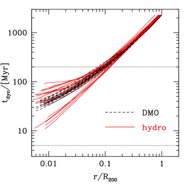
Figure 7: Dynamical time versus radius for DMO (black dashed) and hydro ($n=10$) simulations (red solid). At 1 per cent of the virial radius the dynamical time of the DMO simulations is between 100 and 200 Myr. In order to expand the halo the potential fluctuations (and hence star formation variations) need to occur on a shorter time scale.

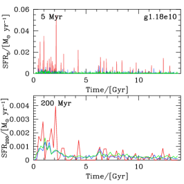
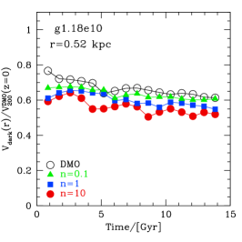
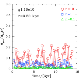
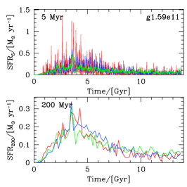
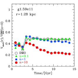
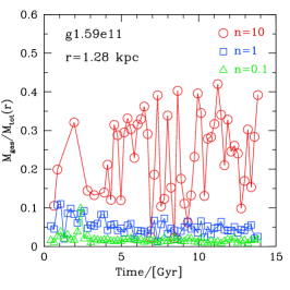
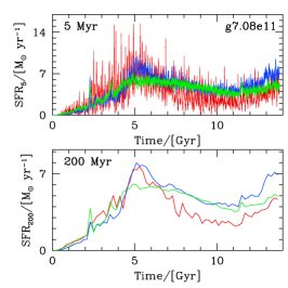
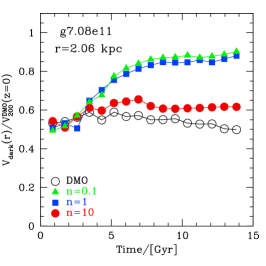
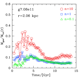
Figure 8: Star formation histories (left panels), dark matter circular velocities (middle panels) and gas fractions (left panels) for three galaxies that show the different types of halo response. A dwarf galaxy g1.18e10 (upper panels), an intermediate mass galaxy g1.59e11 (middle panels), and a milky way mass galaxy g7.08e11 (lower panels). The middle panels show the change in dark matter circular velocity at 1 per cent of the $z=0$ virial radius (this radius is given under the galaxy name). For the star formation histories the upper panels measure star formation in 5 Myr intervals, while the lower panels measure in 200 Myr intervals.

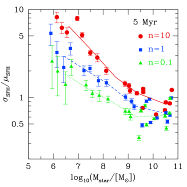
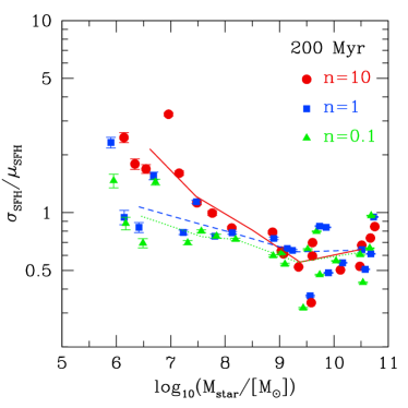
Figure 9: Variability in the star formation history versus $z=0$ stellar mass. The y-axis shows the ratio between standard deviation in SFH to the mean SFH. The error bar corresponds to the Poisson error on the SFR due to the number of star particles formed. Simulations with different star formation thresholds are shown as $n=10$ (red circles), $n=1$ (blue squares), and $n=0.1$ (green triangles). The left panel shows star formation rates measured over 5 Myr intervals, the right panel shows star formation rates measured over 200 Myr intervals. There is more variability in the SFH for lower mass galaxies, higher star formation thresholds, and shorter time scales.

To get a idea of the relevant time scales, Fig. 7 shows the dynamical time $t_{\rm dyn}=\sqrt{3\pi/(16G\overline{\rho})}$ versus radius for DMO simulations (black dashed lines) and hydro simulations with $n=10$ (red solid lines). The dynamical time measures the time it takes to go from a radius $r$ to $r=0$. At 1 per cent of the viral radius the dynamical time varies between 30 and 50 Myr for DMO simulations. For hydro simulations, there is more variation, because some haloes expand (increasing $t_{\rm dyn}$) while others contract (decreasing $t_{\rm dyn}$.). This motivates us to measure the star formation rates on a time scale significantly less than $50$ Myr. Variation of the star formation rates on 100 Myr time scales, as for example adopted by Bose et al. (2018), are not relevant for the role of feedback driven halo expansion.

Observationally different star formation indicators probe different time scales. H$\alpha$ traces star formation within the past $\sim 5$ Myr, while far ultra-violet (FUV) photons trace longer time scales $\sim 100-300$ Myr (Calzetti, 2013). Motivated by this as our default time scales we consider 5 Myr and 200 Myr. On the spatial scales of interest, the former is much smaller than the dynamical time, while the latter is roughly equal to the dynamical time. Recall that in our simulations star formation is computed every 0.84 Myr (Age of universe/$2^{14}$), so we can resolve star formation on a 5 Myr timescale.

5.1 Individual galaxies: test cases

Fig. 8 shows the star formation history (SFH, left), dark matter circular velocity (middle), and gas fractions (right) for three galaxies that have qualitatively different halo responses for $n=10$ (no change, expansion, contraction). The red lines and points show results for $n=10$, blue for $n=1$, and green for $n=0.1$. The SFHs are calculated from the ages of the star particles within the galaxy at redshift $z=0$. We see that the variation in the SFH is strongly dependent on the star formation threshold, the time scale over which we measure the star formation, and the mass of the galaxy. Higher thresholds, shorter time scales, and lower masses result in more bursty SFH. Below we will show that these trends hold for the full sample of 20 haloes.

The middle panel shows the evolution of the dark matter circular velocity at 1 per cent of the $z=0$ virial radius, normalized to the virial velocity of the DMO simulation at $z=0$. Results for DMO simulations (scaled by $\sqrt{1-{f_{\rm bar}}}$) are shown with black circles. The time evolution is typically quite smooth, both when the halo expands and when it contracts. The upper panel shows a dwarf galaxy (g1.18e10) that shows mild expansion for all three thresholds and slightly more expansion for higher $n$. The middle panel shows a galaxy (g1.59e11) that undergoes strong expansion for $n=10$, while hardly any change for $n=1$ and $n=0.1$. The lower panel shows a Milky Way mass galaxy (g7.08e11) which undergoes strong contraction for $n=0.1$ and $n=1$, and mild contraction for $n=10$. We thus see a correlation between the burstiness of star formation on sub-dynamical time scales and the halo response. More bursty SFHs yield lower central dark matter densities, as expected from analytic models (Pontzen & Governato, 2012; Dutton et al., 2016b)

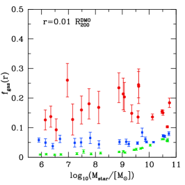
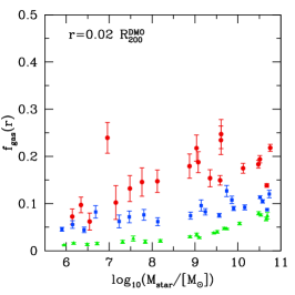
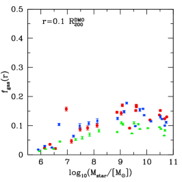
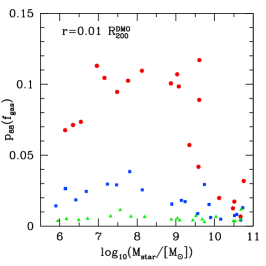
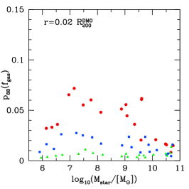
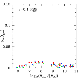
Figure 10: Mean gas fraction (upper panels) and variability in gas fraction (lower panels) versus $z=0$ stellar mass. The colour and symbol type refers to the star formation threshold: $n=10$ (red circles), $n=1$ (blue squares), $n=0.1$ (green triangles). For each galaxy the gas fraction ($f_{\rm gas}(r)=M_{\rm gas}(r)/M_{\rm tot}(r)$) is measured within a fixed physical radius $r$ in the most massive progenitor. The mean gas fraction is averaged over time. The error bars enclose 68 per cent of the variation in $f_{\rm gas}$ about the mean relation versus time. For low threshold ($n=0.1$) the mean and variability in gas fraction are too small to have a meaningful impact on the dark halo structure. For $n=10$ the mean gas fraction is $f_{\rm gas}\simeq 0.2$ and variability $\simeq 0.1$ in haloes that undergo the most expansion.

As discussed above, another key requirement for outflows to expand the halo is for there to be sufficient gas at small radii. The right panels of Fig. 8 show the gas fraction $(M_{\rm gas}/M_{\rm tot})$ measured at 1 per cent of the $z=0$ DMO virial radius. This radius is indicated in the top left corner of the panels and varies from $0.5$ kpc for g1.18e10 to $2.0$ kpc for g7.08e11. We see a clear trend for higher average gas fractions and higher variability for higher star formation thresholds. This is expected since for lower thresholds the gas turns into stars before it can get very dense. We also see that the lowest mass galaxy (g1.18e10) has lower gas fraction variability than the middle mass galaxy (g1.59e11), which qualitatively explains the differences in expansion in these two galaxies. For the Milky Way mass galaxy, the differences in halo contraction start around a time of 3 Gyr. The $n=10$ simulation has significant variations in the gas fraction around this time, which likely prevents the strong contraction that occurs in the low threshold simulations.

5.2 Individual galaxies: full sample

We now expand the results of the previous section to the full sample of 20 haloes. Fig. 9 shows the standard deviation of the SFH, $\sigma_{\rm SFH}$, in units of the mean SFH, $\mu_{\rm SFH}$. This is a measure of how bursty the star formation is, and can be used to quantify analytic SFHs used in interpreting galaxy observations. On a 5 Myr time scale (left panel), there is a roughly constant shift in the scatter between the three thresholds, with more bursty SFH at all masses when the star formation threshold is higher. On a 200 Myr time scale (right panel), there is not much difference in the SFH for galaxies above a stellar mass of $\sim 10^{8}\,{{{\rm M}_{\odot}}}$. Recall that a mass scale of ${{M_{\rm star}}}\sim 10^{9}\,{{{\rm M}_{\odot}}}$ is where there is the most halo expansion. This confirms that variations in star formation (and hence gas fractions) on a dynamical time scale do not play a role in halo expansion. Variations in star formation needs to occur on a sub-dynamical time scale in order to drive a halo response. For both short and long time scales, we see that lower mass galaxies have systematically more bursty SFHs. Comparing this plot with the halo response in Fig. 3 we see that the burstiness of star formation by itself does not determine the halo response, since the lowest mass galaxies have the most bursty SFHs, yet they have no change in the dark matter profile.

We have estimated the uncertainty on the SFH by using the Poisson error on the number of star particles formed. This error is likely an upper limit, because only a fraction of the gas eligible to form stars actually turns into stars. The errors are only significant in the four lowest mass galaxies (${{M_{\rm star}}}<10^{7}{{{\rm M}_{\odot}}}$) and small timescales due to there being only a few thousand star particles formed. The uncertainties are lower for higher $n$, because here the star formation is concentrated into a few bursts, which are well resolved (see top left panel in Fig. 8). While for low $n$, the star formation is roughly uniform in time, and there are only a handful of star formation events in each 5 Myr time interval. We thus conclude that the trend for more bursty star formation in lower mass galaxies is not a manifestation of numerical discreteness.

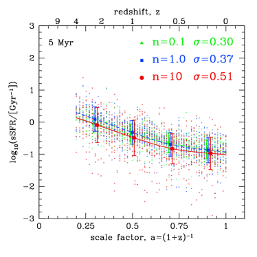
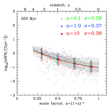
Figure 11: Specific star formation rate versus scale factor. Each small point is a separate galaxy. The large points show the mean sSFR in four scale factor bins. The lines show the interpolated relation with respect to which the standard deviation in $\log_{10}({\rm sSFR})$ is measured. The standard deviation for the different star formation thresholds is given in the top right corner. Star formation rates are measured over a 5 Myr time scale (left), and a 200 Myr time scale (right).

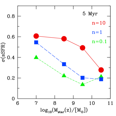
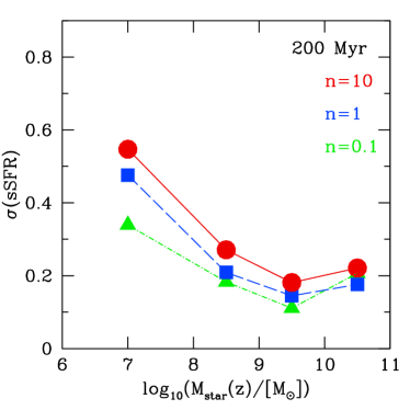
Figure 12: Scatter in specific star formation rate [dex] in bins of stellar mass for populations of galaxies at redshifts $z<4$. Colours and symbols refer to simulations with different star formation thresholds. Star formation rates are measured over a 5 Myr time scale (left), and a 200 Myr time scale (right).

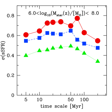
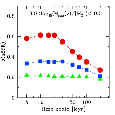
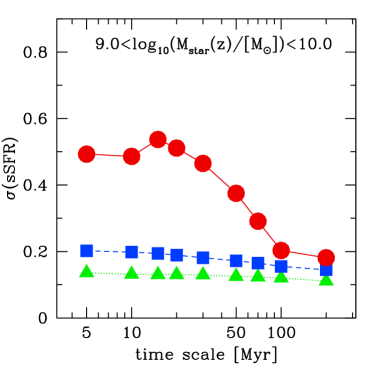
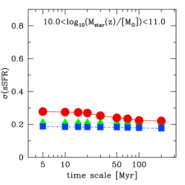
Figure 13: Scatter in specific star formation rate [dex] versus time scale over which star formation rate is measured. Each panel corresponds to a different range in stellar masses, ${{M_{\rm star}}}(z)$, as indicated. Colours and symbols refer to simulations with different star formation thresholds: $n=10$ (red circles, solid lines); $n=1$ (blue squares, dashed lines); and $n=0.1$ (green triangles, dotted lines).

The recent SFHs of individual galaxies can be constrained using the ratio of H$\alpha$ to FUV fluxes (Weisz et al., 2012; Sparre et al., 2017) or a combination of the 4000Å  break, H$\delta_{A}$ indices and specific star formation rate SFR$/{{M_{\rm star}}}$ (Kauffmann, 2014). The general conclusion from observations is that lower mass galaxies have more bursty recent SFHs. This is qualitatively consistent with our simulations with all $n$, and also the FIRE simulations (Sparre et al., 2017), which have a high $n$.

Fig. 10 shows the mean (upper panels) and variability (lower panels) of gas fractions (measured over cosmic time) versus the stellar mass at $z=0$. The gas fraction $f_{\rm gas}(r)=M_{\rm gas}(r)/M_{\rm tot}(r)$ is measured within a fixed physical radius. Each point corresponds to the evolution of a single galaxy. The radii are 1 per cent (left), 2 per cent (middle), and 10 per cent (right) of the $z=0$ DMO virial radius. The variability is defined as enclosing 68% of the points about the mean. This plot explains the differences in halo response we see between different $n$, as well as at different radii. At large radii (10 per cent of the virial radius), there is less than 2 per cent variability in $f_{\rm gas}$ for all galaxy masses and star formation thresholds. Recall, that the expansive effects of gas outflows go like the square of the outflow fraction, so we expect no expansive effects at large radii. Thus on these scales the dark halo structure will be determined by the adiabatic contraction due to inflows. At smaller radii we see higher gas fractions and variability for $n=10$, but lower gas fractions and variability for lower thresholds. For $n=10$ the trend of variability with mass follows the trend of halo response with mass seen in Fig. 3. For $n=0.1$ the variability is less than a per cent, which explains why we see no halo expansion in low mass galaxies, in spite of there being some scatter in the SFHs.

Note that the time scale at which we are measuring variation (in gas fractions) is limited by the frequency $\simeq 215\,$Myr of the simulation outputs. At small radii this is not a sub-dynamical time. We have tested a few simulations with more outputs, from which we see sudden drops in gas fractions occurring on $\sim 25\,$Myr time scales. However, the scatter about the mean gas fraction is comparable when we use 13 Myr between outputs, or our default of $215\,$Myr. Note that the SFHs in Figs. 8 and 9 are measured from the birth time of the star particles and are thus not effected by the output frequency.

5.3 Star formation rates for samples of galaxies

In order to probe the variability in star formation on short time scales $\sim 10$ Myr, one can resort to samples of galaxies. For samples of galaxies one can observationally measure the scatter in the star formation rate versus stellar mass relation, or equivalently the specific star formation rate, sSFR$=$SFR$/{{M_{\rm star}}}$. Fig. 11 shows the evolution of sSFR for the main galaxy in each of the 20 simulations, for $z<4$, sSFR$>0.001$ Gyr^-1, and for ${{M_{\rm star}}}(z)>10^{6}\,{{{\rm M}_{\odot}}}$. The points are colour coded by the star formation threshold. The large points show means in bins of scale factor. The lines are spline interpolations of the mean with respect to which we measure the standard deviation, $\sigma(\log_{10}{\rm sSFR})$. The error bars show the scatter in 4 redshift bins, showing minimal redshift dependence. On 200 Myr time scales (right panel), the scatter for $n=10$ and $n=1$ is the same ($\simeq 0.38$ dex) and 0.1 dex larger than for $n=0.1$. On a 5 Myr time scale (left panel), there is a 0.2 dex difference in the scatter for $n=10$ and $n=0.1$.

The mass dependence of the scatter is shown in Fig. 12 for a time scale of 5 (left) and 200 Myr (right). Similar to Fig. 9, we see that there is more variation in the sSFR in lower mass galaxies, shorter time scales, and higher star formation thresholds. The differences with respect to the star formation threshold are most pronounced at the stellar masses ($10^{8}\mathrel{\hbox to0.0pt{\lower 3.0pt\hbox{$\sim$}\hss}\raise 2.0pt\hbox{$<$}}{{M_{\rm star}}}\mathrel{\hbox to0.0pt{\lower 3.0pt\hbox{$\sim$}\hss}\raise 2.0pt\hbox{$<$}}10^{10}\,{{{\rm M}_{\odot}}}$), where interestingly the most expansion occurs for $n=10$ simulations. There is a large difference (0.4 dex) in scatter between $n=10$ and $n=0.1$ simulations on 5 Myr time scales, but just a 0.1 dex difference for a 200 Myr time scale.

In order to determine the characteristic time scale for variability in star formation in Fig. 13, we plot the scatter in sSFR versus the time scale the star formation rate is measured over, ranging from 5 Myr to 200 Myr, and in 4 bins of stellar mass (as indicated). For all time scales and stellar masses, $n=10$ simulations have larger scatter than both $n=1$ and $n=0.1$. The scatter peaks at a $\sim 20$ Myr time scale, which indicates the characteristic time scale for episodes of star formation in the NIHAO simulations.

6 Summary

We use 20 sets of cosmological hydrodynamical simulations from the NIHAO project (Wang et al., 2015) to investigate the impact of the star formation threshold, $n$, on the response of the dark matter halo to galaxy formation. We consider three values: $n=10[{\rm cm}^{-3}]$ (the fiducial NIHAO), $n=1$, and $n=0.1$. The masses of the central dark matter haloes in our study cover the range $10^{10}\mathrel{\hbox to0.0pt{\lower 3.0pt\hbox{$\sim$}\hss}\raise 2.0pt\hbox{$<$}}M_{200}\mathrel{\hbox to0.0pt{\lower 3.0pt\hbox{$\sim$}\hss}\raise 2.0pt\hbox{$<$}}10^{12}\,{{{\rm M}_{\odot}}}$ at redshift $z=0$. We summarize our results as follows:

• For the $n=10$ and $n=1$ simulations the stellar to halo mass relations are consistent with halo abundance matching for redshifts $z<4$, without modification of any other parameter (Fig. 1). For the $n=0.1$ simulations the feedback is too efficient, resulting in stellar masses that are too low. This is easily fixed by reducing the feedback efficiency from young stars from 0.13 to 0.04.

• The dark matter density profiles at redshift $z=0$ show significant departures from dissipationless DMO simulations (Fig. 2), with both contraction and expansion.

• The halo response at small radii ($\sim 1$ per cent of the virial radius) is more strongly correlated with ${{M_{\rm star}}}/M_{200}$ than either stellar mass or halo mass alone for all $n$ (Fig. 3).

• Simulations with $n=0.1$ do not result in halo expansion (beyond adiabatic mass loss) at any mass scale we study (Fig. 2). Simulations with $n=1$ largely follow the halo response of $n=0.1$, but with a small amount of expansion at $0.001\mathrel{\hbox to0.0pt{\lower 3.0pt\hbox{$\sim$}\hss}\raise 2.0pt\hbox{$<$}}{{M_{\rm star}}}/M_{200}\mathrel{\hbox to0.0pt{\lower 3.0pt\hbox{$\sim$}\hss}\raise 2.0pt\hbox{$<$}}0.01$. Simulations with $n=10$ result in strong expansion for $0.001\mathrel{\hbox to0.0pt{\lower 3.0pt\hbox{$\sim$}\hss}\raise 2.0pt\hbox{$<$}}{{M_{\rm star}}}/M_{200}\mathrel{\hbox to0.0pt{\lower 3.0pt\hbox{$\sim$}\hss}\raise 2.0pt\hbox{$<$}}0.01$ and weaker contraction (than $n=0.1$) for ${{M_{\rm star}}}/M_{200}\mathrel{\hbox to0.0pt{\lower 3.0pt\hbox{$\sim$}\hss}\raise 2.0pt\hbox{$>$}}0.3$ (Fig. 3).

• Field galaxies in the local group with stellar masses $10^{6}\mathrel{\hbox to0.0pt{\lower 3.0pt\hbox{$\sim$}\hss}\raise 2.0pt\hbox{$<$}}{{M_{\rm star}}}\mathrel{\hbox to0.0pt{\lower 3.0pt\hbox{$\sim$}\hss}\raise 2.0pt\hbox{$<$}}10^{8}{{{\rm M}_{\odot}}}$ have circular velocities at the half-light radius consistent with $n=10$ simulations, but a factor of $\simeq 1.4$ lower than $n=0.1$ simulations (Fig. 4).

• Field galaxies with stellar masses $10^{9}\mathrel{\hbox to0.0pt{\lower 3.0pt\hbox{$\sim$}\hss}\raise 2.0pt\hbox{$<$}}{{M_{\rm star}}}\mathrel{\hbox to0.0pt{\lower 3.0pt\hbox{$\sim$}\hss}\raise 2.0pt\hbox{$<$}}10^{10}{{{\rm M}_{\odot}}}$ have dark matter circular velocities at 2 kpc a factor of $1.5$ lower than predicted by $n=1$ and $n=0.1$ simulations but a factor of $1.15$ higher than $n=10$ simulations (Fig. 5).

• For Milky Way mass galaxies, the simulations are consistent with the observed circular velocity at 8 kpc and 60 kpc. All haloes contract, with more contraction at smaller radii. Simulations with $n=0.1$ and $n=1$ have almost identical halo contraction, while simulations with $n=10$ have a factor $\sim 2$ less contraction at small scales (Fig. 6).

• Lower $n$ simulations have lower mean, and lower variability in the gas fractions within small radii (Figs. 8 & 10). For the galaxies that experience the most halo expansion in the $n=10$ simulations the variations in gas fractions are $\simeq 0.1$. Each such outflow and inflow cycle is expected to expand the dark matter orbits by roughly a per cent, so many such cycles are required to significantly expand the dark matter halo. For the $n=0.1$ simulations the variability in gas fractions is $\sim 0.01$, and so the expansive effect of each cycle is $\sim 10^{-4}$, and thus negligible. The average gas fractions and the variability in the gas fractions (for populations of galaxies) could be measured with radio observations.

• Star formation is more bursty in lower mass galaxies, and for simulations with higher $n$ (Figs. 9 & 12).

• For star formation feedback to drive halo expansion the variability must occur on a sub-dynamical time scale (i.e., much less than 50 Myr at one percent of the virial radius). Measuring star formation rates on a 100 Myr time scale, as done by Bose et al. (2018), is thus not relevant to the problem of feedback driven halo expansion.

• For $n=0.1$ simulations the scatter in sSFR is only weakly dependent on the time scale over which the SFR is measured. However, for $n=10$ simulations, shorter time scales result in larger scatter down to a characteristic time scale of $\sim 20$ Myr (Fig. 13).

• Bursty star formation on a short time scale is a necessary but not sufficient condition for halo expansion to occur. This is readily apparent when one sees that the lowest mass galaxies we simulate ${{M_{\rm star}}}\sim 10^{6}{{{\rm M}_{\odot}}}$ have the most bursty star formation (Fig. 9), yet the halo response is weak (Fig. 3).

• At the stellar mass range that undergoes the most halo expansion $10^{8}\mathrel{\hbox to0.0pt{\lower 3.0pt\hbox{$\sim$}\hss}\raise 2.0pt\hbox{$<$}}{{M_{\rm star}}}\mathrel{\hbox to0.0pt{\lower 3.0pt\hbox{$\sim$}\hss}\raise 2.0pt\hbox{$<$}}10^{9}\,{{{\rm M}_{\odot}}}$, there is 0.4 dex more scatter in the sSFR (when measured on $\mathrel{\hbox to0.0pt{\lower 3.0pt\hbox{$\sim$}\hss}\raise 2.0pt\hbox{$<$}}20$ Myr time scales) for $n=10$ simulations compared to $n=0.1$ simulations (Fig. 13). In principle star formation rates on these time scales could be measured with H$\alpha$ emission, provided that extinction does not impact the scatter in sSFR too severely.

Our study reconciles the conflicting results in the literature from cosmological simulations for how the dark matter halo responds to galaxy formation. In addition to the ratio between stellar mass and halo mass (e.g., Di Cintio et al., 2014a), we have shown that the halo response is a strong function of the star formation threshold. Simulations that use low star formation thresholds ($n\mathrel{\hbox to0.0pt{\lower 3.0pt\hbox{$\sim$}\hss}\raise 2.0pt\hbox{$<$}}0.1$), such as EAGLE (Schaye et al., 2015) find no significant change in haloes of mass $10^{10}$ and $10^{11}{{{\rm M}_{\odot}}}$, and mild contraction in haloes of mass $10^{12}{{{\rm M}_{\odot}}}$ (Schaller et al., 2015; Bose et al., 2018). This is exactly the same as we find for our $n=0.1$ simulations. Simulations with high star formation thresholds ($n\mathrel{\hbox to0.0pt{\lower 3.0pt\hbox{$\sim$}\hss}\raise 2.0pt\hbox{$>$}}10$) such as Governato et al. (2010); Di Cintio et al. (2014a); Tollet et al. (2016); Chan et al. (2015) result in halo expansion in dwarf galaxies (halo masses $\sim 10^{10}$ to $\sim 10^{11}{{{\rm M}_{\odot}}}$) and contraction in Milky Way mass haloes ($\sim 10^{12}{{{\rm M}_{\odot}}}$).

A similar conclusion has been reached independently by Benitez-Llambay et al. (2018) using simulations with the EAGLE code. These authors take the dependence of halo structure on the star formation threshold with a pessimistic view of being able to predict the structure of CDM haloes. We are more optimistic, because we have shown that there are large differences in the gas fractions and star formation rates in simulations with different star formation thresholds. Thus it should be possible in the near future to observationally distinguish between different star formation thresholds, and more generally to calibrate the free parameters of the sub-grid model for star formation and feedback.

Indeed, in Buck et al. (2018) we use our simulations to show that the spatial clustering strength of young stars depends on the star formation threshold. The observed clustering from the HST Legacy Extragalactic UV Survey (LEGUS Grasha et al., 2017) is inconsistent with a low threshold ($n<1$ [cm^-3]) and strongly favours a high threshold ($n>10$ [cm^-3]).

References

- Behroozi et al. (2013) Behroozi, P. S., Wechsler, R. H., & Conroy, C. 2013, ApJ, 770, 57
- Benitez-Llambay et al. (2018) Benitez-Llambay, A., Frenk, C. S., Ludlow, A. D., & Navarro, J. F. 2018, arXiv:1810.04186
- Blumenthal et al. (1986) Blumenthal, G. R., Faber, S. M., Flores, R., & Primack, J. R., 1986, ApJ, 301, 27
- Bose et al. (2018) Bose, S., Frenk, C. S., Jenkins, A., et al. 2018, arXiv:1810.03635
- Bovy & Rix (2013) Bovy, J., & Rix, H.-W. 2013, ApJ, 779, 115
- Buck et al. (2017) Buck, T., Macciò, A. V., Obreja, A., et al. 2017, MNRAS, 468, 3628
- Buck et al. (2018) Buck, T., Macciò, A. V., Dutton, A. A., Obreja, A., & Frings, J. 2018, MNRAS in press, arXiv:1804.04667
- Buck et al. (2018) Buck, T., Dutton, A. A., & Macciò, A. V. 2018, arXiv:1812.05613
- Bullock & Boylan-Kolchin (2017) Bullock, J. S., & Boylan-Kolchin, M. 2017, ARA&A, 55, 343
- Calzetti (2013) Calzetti, D. 2013, Secular Evolution of Galaxies, 419
- Chan et al. (2015) Chan, T. K., Kereš, D., Oñorbe, J., et al. 2015, MNRAS, 454, 2981
- Crain et al. (2015) Crain, R. A., Schaye, J., Bower, R. G., et al. 2015, MNRAS, 450, 1937
- Dalla Vecchia & Schaye (2012) Dalla Vecchia, C., & Schaye, J. 2012, MNRAS, 426, 140
- Di Cintio et al. (2014a) Di Cintio, A., Brook, C. B., Macciò, A. V., et al. 2014, MNRAS, 437, 415
- Dutton et al. (2011) Dutton, A. A., Conroy, C., van den Bosch, F. C., et al. 2011, MNRAS, 416, 322
- Dutton & Macciò (2014) Dutton, A. A., & Macciò, A. V. 2014, MNRAS, 441, 3359
- Dutton et al. (2016a) Dutton, A. A., Macciò, A. V., Frings, J., et al. 2016a, MNRAS, 457, L74
- Dutton et al. (2016b) Dutton, A. A., Macciò, A. V., Dekel, A., et al. 2016b, MNRAS, 461, 2658
- Dutton et al. (2017) Dutton, A. A., Obreja, A., Wang, L., et al. 2017, MNRAS, 467, 4937
- Dutton et al. (2019) Dutton, A. A., Obreja, A., & Macciò, A. V. 2019, MNRAS, 482, 5606
- El-Zant et al. (2001) El-Zant, A., Shlosman, I., & Hoffman, Y. 2001, ApJ, 560, 636
- Garrison-Kimmel et al. (2014) Garrison-Kimmel, S., Boylan-Kolchin, M., Bullock, J. S., & Kirby, E. N. 2014, MNRAS, 444, 222
- Gill et al. (2004) Gill, S. P. D., Knebe, A., & Gibson, B. K. 2004, MNRAS, 351, 399
- Gnedin et al. (2004) Gnedin, O. Y., Kravtsov, A. V., Klypin, A. A., & Nagai, D. 2004, ApJ, 616, 16
- Governato et al. (2010) Governato, F., Brook, C., Mayer, L., et al. 2010, Nature, 463, 203
- Grand et al. (2017) Grand, R. J. J., Gómez, F. A., Marinacci, F., et al. 2017, MNRAS, 467, 179
- Grasha et al. (2017) Grasha, K., Calzetti, D., Adamo, A., et al. 2017, ApJ, 840, 113
- Gutcke et al. (2017) Gutcke, T. A., Stinson, G. S., Macciò, A. V., Wang, L., & Dutton, A. A. 2017, MNRAS, 464, 2796
- Hopkins et al. (2014) Hopkins, P. F., Kereš, D., Oñorbe, J., et al. 2014, MNRAS, 445, 581
- Hopkins et al. (2018) Hopkins, P. F., Wetzel, A., Kereš, D., et al. 2018, MNRAS, 480, 800
- Kauffmann (2014) Kauffmann, G. 2014, MNRAS, 441, 2717
- Kirby et al. (2014) Kirby, E. N., Bullock, J. S., Boylan-Kolchin, M., Kaplinghat, M., & Cohen, J. G. 2014, MNRAS, 439, 1015
- Knollmann & Knebe (2009) Knollmann, S. R., & Knebe, A. 2009, ApJS, 182, 608
- Lelli et al. (2016) Lelli, F., McGaugh, S. S., & Schombert, J. M. 2016, AJ, 152, 157
- Macciò et al. (2012) Macciò, A. V., Stinson, G., Brook, C. B., et al. 2012, ApJ, 744, L9
- Macciò et al. (2016) Macciò, A. V., Udrescu, S. M., Dutton, A. A., et al. 2016, MNRAS, 463, L69
- Marinacci et al. (2014) Marinacci, F., Pakmor, R., & Springel, V. 2014, MNRAS, 437, 1750
- Moster et al. (2013) Moster, B. P., Naab, T., & White, S. D. M. 2013, MNRAS, 428, 3121
- Moster et al. (2018) Moster, B. P., Naab, T., & White, S. D. M. 2018, MNRAS, 477, 1822
- Oman et al. (2015) Oman, K. A., Navarro, J. F., Fattahi, A., et al. 2015, MNRAS, 452, 3650
- Oman et al. (2019) Oman, K. A., Marasco, A., Navarro, J. F., et al. 2019, MNRAS, 482, 821
- Planck Collaboration et al. (2014) Planck Collaboration, Ade, P. A. R., Aghanim, N., et al. 2014, A&A, 571, A16
- Pontzen & Governato (2012) Pontzen, A., & Governato, F. 2012, MNRAS, 421, 3464
- Power et al. (2003) Power, C., Navarro, J. F., Jenkins, A., et al. 2003, MNRAS, 338, 14
- Rahmati et al. (2013) Rahmati, A., Schaye, J., Pawlik, A. H., & Raičevi, M. 2013, MNRAS, 431, 2261
- Read & Gilmore (2005) Read, J. I., & Gilmore, G. 2005, MNRAS, 356, 107
- Read et al. (2016) Read, J. I., Agertz, O., & Collins, M. L. M. 2016, MNRAS, 459, 2573
- Santos-Santos et al. (2018) Santos-Santos, I. M., Di Cintio, A., Brook, C. B., et al. 2018, MNRAS, 473, 4392
- Sawala et al. (2016) Sawala, T., Frenk, C. S., Fattahi, A., et al. 2016, MNRAS, 457, 1931
- Schaller et al. (2015) Schaller, M., Frenk, C. S., Bower, R. G., et al. 2015, MNRAS, 451, 1247
- Schaye et al. (2015) Schaye, J., Crain, R. A., Bower, R. G., et al. 2015, MNRAS, 446, 521
- Semenov et al. (2017) Semenov, V. A., Kravtsov, A. V., & Gnedin, N. Y. 2017, ApJ, 845, 133
- Simard et al. (2011) Simard, L., Mendel, J. T., Patton, D. R., Ellison, S. L., & McConnachie, A. W. 2011, ApJS, 196, 11
- Sparre et al. (2017) Sparre, M., Hayward, C. C., Feldmann, R., et al. 2017, MNRAS, 466, 88
- Stadel et al. (2009) Stadel, J., Potter, D., Moore, B., et al. 2009, MNRAS, 398, L21
- Stinson et al. (2006) Stinson, G., Seth, A., Katz, N., et al. 2006, MNRAS, 373, 1074
- Stinson et al. (2013) Stinson, G. S., Brook, C., Macciò, A. V., et al. 2013, MNRAS, 428, 129
- Stinson et al. (2015) Stinson, G. S., Dutton, A. A., Wang, L., et al. 2015, MNRAS, 454, 1105
- Teyssier et al. (2013) Teyssier, R., Pontzen, A., Dubois, Y., & Read, J. I. 2013, MNRAS, 429, 3068
- Tollet et al. (2016) Tollet, E., Macciò, A. V., Dutton, A. A., et al. 2016, MNRAS, 456, 3542
- Valenzuela et al. (2007) Valenzuela, O., Rhee, G., Klypin, A., et al. 2007, ApJ, 657, 773
- Vogelsberger et al. (2014) Vogelsberger, M., Genel, S., Springel, V., et al. 2014, MNRAS, 444, 1518
- Wang et al. (2015) Wang, L., Dutton, A. A., Stinson, G. S., et al. 2015, MNRAS, 454, 83
- Wadsley et al. (2017) Wadsley, J. W., Keller, B. W., & Quinn, T. R. 2017, MNRAS, 471, 2357
- Weinberg & Katz (2002) Weinberg, M. D., & Katz, N. 2002, ApJ, 580, 627
- Weisz et al. (2012) Weisz, D. R., Johnson, B. D., Johnson, L. C., et al. 2012, ApJ, 744, 44
- Widrow et al. (2008) Widrow, L. M., Pym, B., & Dubinski, J. 2008, ApJ, 679, 1239-1259
- Xue et al. (2008) Xue, X. X., Rix, H. W., Zhao, G., et al. 2008, ApJ, 684, 1143