On some properties of the new Sine-skewed Cardioid Distribution

Abstract.

The new Sine Skewed Cardioid (ssc) distribution been just introduced and characterized by Ahsanullah (2018). Here, we study the asymptotic properties of its tails by determining its extreme value domain, the characteristic function, the moments and likelihood estimators of the two parameters, the asymptotic normality of the moments estimators and the random generation of data from the ssc distribution. Finally, we proceed to a simulation study to show the performance of the random generation method and the quality of the moments estimation of the parameters.

⁽¹⁾ Cherif Mamadou Moctar Traoré.
Université des Sciences, des Technique et des Technologies, Bamako, Mali
Email : cheriftraore75@yahoo.com

⁽²⁾ Moumouni Diallo
Université des Scences Economiques et de Gestion (USEG), Bamako, Mali.
Email : moudiallo1@gmail.com.

⁽³⁾ Gane Samb Lo.
LERSTAD, Gaston Berger University, Saint-Louis, Sénégal (main affiliation).
LSTA, Pierre and Marie Curie University, Paris VI, France.
AUST - African University of Sciences and Technology, Abuja, Nigeria
gane-samb.lo@edu.ugb.sn, gslo@aust.edu.ng, ganesamblo@ganesamblo.net
Permanent address : 1178 Evanston Dr NW T3P 0J9,Calgary, Alberta, Canada.

⁽⁴⁾ Mouhamad Ahsanullah
Department of Management Sciences. Rider University. Lawrenceville, New Jersey, USA
Email : ahsan@rider.edu

⁽⁵⁾ Okereke Lois Chinwendu
AUST - African University of Sciences and Technology, Abuja, Nigeria
Email : lokereke@aust.edu.ng.

1. Introduction

Ahsanullah (2018) introduced the new distribution with probability distribution function (pdf)

$$f(x)=\frac{1}{2\pi}(1+\lambda\sin x)(1+\rho\cos x)1_{\left[-\pi,\pi\right]},$$

associated with the parameters $(\lambda,\rho)\in\left[-1,1\right]^{2}$ and named as the sine-skewed cardioid distribution.

In this note, we will state a number properties of that new law. In particular, we are going asymptotic properties of its tails by determining its extreme value domain, the moments and likelihood estimators of the two parameters, the asymptotic normality of the moments estimators and the random generation of data from the ssc distribution. But, before we proceed, we recall for Ahsanullah (2018) that the cumulative distribution function (cdf) is

$$F(x)=\frac{1}{2}+\frac{1}{2\pi}\left(x-\lambda(\cos x+1)+\rho\sin x-\frac{\lambda\rho}{4}(\cos 2x-1)\right),\ x\in\left[-\pi,\pi\right].$$

To prepare studying the upper tail (in a neighborhood of $\pi$) and the lower tail (in a neighborhood of $-\pi$), we may write, respectively, for $x\in\left[-\pi,\pi\right]$,

(1.1) $$F(x)=1-\frac{1}{2\pi}\left((\pi-x)-\lambda(\cos x+1)+\rho\sin(\pi-x)-\frac{\lambda\rho}{4}(\cos 2x-1)\right)$$

and

(1.2) $$F(x)=\frac{1}{2\pi}\left((x+\pi)-\lambda(\cos x+1)-\rho\sin(\pi+x)-\frac{\lambda\rho}{4}(\cos 2x-1)\right).$$

We will have to deal with some statistical properties. So, we suppose that we have a sequence $X$, $X_{1}$, $X_{2}$, $\cdots$, etc. of real-valued random variables defined on the same probability space $(\Omega,\mathcal{A},\mathbb{P}$ with cdf $F$, then supported by $[-\pi,\pi]$. We define the sequence of empirical maxima and the minim

$$X_{1,n}=\min(X_{1},\cdots,X_{n})\ and\ X_{n,n}=\max(X_{1},\cdots,X_{n}),\ n\geq 1$$

and the empirical moments

$$\overline{X}_{n}=\frac{1}{n}\sum_{1\leq j\leq n}X_{j}\ ,\ S_{n}^{2}=\frac{1}{n-1}\sum_{1\leq j\leq n}\left(X_{j}-\overline{X}_{n}\right)^{2},\ n\geq 2$$

and the non-centered second moment

$$m_{2,n}=\frac{1}{n}\sum_{1\leq j\leq n}X_{j}^{2}.$$

Some graphical illustrations of the pdf for some values of the parameters $(\lambda,\rho)$ are also given by Ahsanullah (2018) in Figure 2

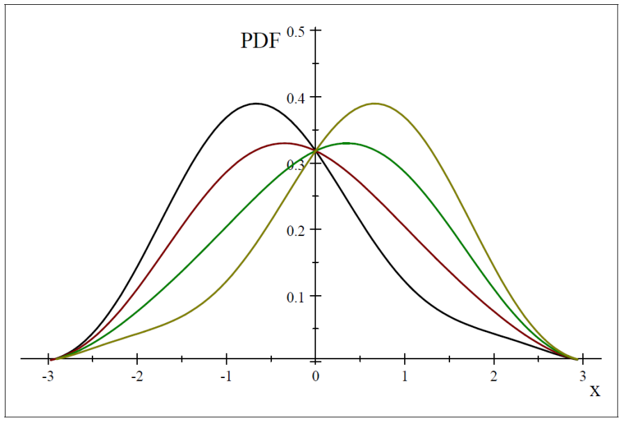
Figure 1. PDF of $f_{sc}(x,1,\lambda),$Black-$\lambda=-0.6$, Red- $\lambda=-0.2$, Green-$\lambda=0.2$ and Brown-$\lambda=0.6$

The rest of the paper is organized as follows. Section 2 is devoted a study of the extreme behavior the the tails of the ssc cdf. In Section 3, we deal with the moments and likelihood estimation of the parameters $\lambda$ and $\rho$ and determine the asymptotic laws of the moments estimators. In Section 4, we provide the characteristic function. Finally, in Section 5, we propose a method of generating samples from the ssc model. Simulation studies are undertaken to test the generation algorithm and next to test the performance of the moments estimators. VB6 Subroutines for the generation methods are given in the appendix. The paper ends by a conclusion section.

2. Asymptotic Properties of the tails

Theorem 1.

Define the constants

$$2\pi\alpha_{1} = 1+\rho,\ 2\pi\alpha_{2}=\frac{\lambda}{2}\left(1-\rho\right),\ 2\pi\alpha_{3}=-\frac{\rho}{6}$$

$$2\pi\alpha_{4} = \frac{\lambda}{24}\left(4\rho-1\right),\ 2\pi\alpha_{5}=\frac{\rho}{120},\ 2\pi\alpha_{6}=\frac{\lambda}{126}\left(1-16\rho\right).$$

We have, as $x\rightarrow\pi,$

$$\frac{\alpha_{5}}{\alpha_{6}(\pi-x)}\left(\frac{\alpha_{4}}{\alpha_{5}(\pi-x)}\left(\frac{\alpha_{3}}{\alpha_{4}(\pi-x)}\left(\frac{\alpha_{3}}{\alpha_{2}(\pi-x)}\left(\frac{\alpha_{1}}{\alpha_{2}(\pi-x)}\right.\right.\right.\right.$$

$$\left.\left.\left.\left.\left(\frac{1-F(x)}{\alpha_{1}(\pi-x)}\right)-1\right)-1\right),-1\right)-1\right)-1=O(\pi-x)$$

and as $x\rightarrow-\pi$,

$$\frac{\alpha_{5}}{\alpha_{6}(\pi+x)}\left(\frac{\alpha_{4}}{\alpha_{5}(\pi+x)}\left(\frac{\alpha_{3}}{\alpha_{4}(\pi+x)}\left(\frac{\alpha_{3}}{\alpha_{2}(\pi+x)}\left(\frac{\alpha_{1}}{\alpha_{2}(\pi+x)}\right.\right.\right.\right.$$

$$\left.\left.\left.\left.\left(\frac{F(x)}{\alpha_{1}(\pi+x)}\right)-1\right)-1\right)-1\right)-1\right)-1=O(\pi+x).$$

Remark : Such an expansion is limited to an order 6. But it might be given an any order $k\geq 2.$

Proof of Theorem 2. We only give elements for the proof of the first. We use the following elementary expansions

$$\sin(\pi-x) = \sum_{k=0}^{\infty}\frac{(-1)^{k+1}}{(2k+1)!}(\pi-x)^{2k+1}$$

$$\cos x+1 = \cos x-\cos\pi=\sum_{k=1}^{\infty}\frac{(-1)^{k+1}}{(2k)!}(\pi-x)^{2k}$$

$$\cos 2x-1 = \cos 2x-\cos 2\pi=\sum_{k=1}^{\infty}(-1)^{k}\frac{2^{2k}}{(2k)!}(x-\pi)^{2k}.$$

We consider the limited expansion at order 6 at $\pi$ to have

$$1-F(x) = \alpha_{1}(\pi-x)+\alpha_{2}(\pi-x)^{2}+\alpha_{3}(\pi-x)^{3}+2\pi\alpha_{4}(\pi-x)^{4}$$

$$+\alpha_{5}(\pi-x)^{5}+\alpha_{6}(\pi-x)^{6}+O((\pi-x)^{7}.$$

This justifies the expansion at $+\pi$. The situation is the same at $-\pi$ from Formula . The reason is that $+\pi$ and $-\pi$ play the same roles in the developments and the two terms $-\rho\sin(\pi+\theta)$ and $\rho\sin(\pi-\theta)$ are expanded in the same way with respect to $\pi-x$ and $\pi+x$ respectively. $\square$

From Theorem 2, we directly get the extreme law of $X$ and $Y=1/(\pi+X)$.

Theorem 2.

We have the following properties

(a) $F^{\star}(x)=F(\pi-\frac{1}{x}),x>0$ belong to the Frechet extreme value Domain $D(H_{1})$ that is

$$\forall\gamma>0,\text{ }\lim_{x\rightarrow+\infty}\frac{1-F^{\star}(\gamma x)}{1-F^{\star}(x)}=\gamma^{-1}$$

and the second order condition

$$\forall\gamma>0,\text{ }\lim_{x\rightarrow+\infty}\frac{1}{S(x)}\left(\frac{1-F^{\star}(\gamma x)}{1-F^{\star}(x)}-\gamma^{-1}\right)=0$$

for $S(x)=\alpha_{2}x/\alpha_{1}$, $x>0$.

b) As a consequence $F$ is in the Weibull extreme value Domain $D(H_{-1})$ and we have

$$n(1+\rho)\left(X_{n,n}-\pi\right)\rightsquigarrow H_{-1},\ as\ n\rightarrow\infty.$$

(c) To have the extreme lower law is found by using $X_{1,n}=-(-X)_{n,n}$ and $(-X)_{n,n}$ and $X_{n,n}$ have the same limit in type, that is

$$n(1+\rho)\left((-X)_{n,n}-\pi\right)\rightsquigarrow H_{-1},\ as\ n\rightarrow\infty.$$

Proof of Theorem 2. Point (a) is a direct consequence of Theorem at the first order. By Theorem 8 in Lo (2018b), we have that $F\in D(H_{1})$ if and only if $F^{\ast}\in D(H_{-1})$. So (b) holds from (a). Furthermore, by Proposition 8 in Lo (2018b), we also have

(2.1) $$\frac{X_{n,n}-uep(F)}{uep(F)-F^{-1}(1-1/n))}\rightsquigarrow H_{-1},\ as\ n\rightarrow\infty.$$

Now from the expansions in Theorem , we have for any $-1<u<1$

$$1-F(x)=u$$

$$\Leftrightarrow \alpha_{1}(\pi-x)+\alpha_{2}(\pi-x)^{2}+...+\alpha_{6}(\pi-x)^{6}+O((\pi-x)^{7}).$$

We get that, as $x\rightarrow+\pi$,

$$(\pi-x)\sim u/\alpha_{1},$$

and

$$x=F^{-1}(1-u)=\pi-\frac{1}{\alpha_{1}}u+\frac{\alpha_{2}}{\alpha_{1}^{3}}u^{2}(1+\varepsilon_{2}(1))+\cdots+\frac{\alpha_{6}}{\alpha_{1}^{7}}u^{6}(1+\varepsilon_{6}(1))+O(u^{7}),$$

where the function $\varepsilon_{h}(u)$ go to zero as $u\downarrow 0$. In particular, we have

$$\pi-F^{-1}(1-u)\sim\frac{1}{\alpha_{1}}u=\frac{u}{1+\rho}$$

and, as $n\rightarrow+\infty$

$$\pi-F^{-1}(1-1/n)\sim\frac{1}{\alpha_{1}}=\frac{1}{n(1+\rho)},$$

which combined with Formula 2.1 concludes Point (b) of the proof.

Point (c) is based the cdf of $-X$, which is $F^{\bot}(x)=1-F(-x)$, for $-\pi\leq x\leq\pi$. And the expansion of $1-F^{\bot}(x)$ gives the same expansion as in Formula at $+\pi$. We get the same conclusion as for $X$. $\blacksquare$

Interesting Pedagogical Example. As we can find in Lo (2018b), page 133, a criterion of belonging of $F$ to $D(H_{1})$, when $uep(F)=\pi$ is that $F$ admits a derivative in a right neighborhood of $\pi$ and that

(2.2) $$\lim_{x\rightarrow\pi}\frac{(\pi-x)F^{\prime}(x)}{1-F(x)}=1.$$

It is also stated that the condition 2.2 holds if $F\in D(H_{1})$ and $F^{\prime}$ is ultimately non-increasing as $x\nearrow\pi$. Here, the limit holds for all values of $\lambda$ and $\rho$ in $]-1,1[$ although $F^{\prime}$ is ultimately not non-increasing for some values of $\lambda$ and $\rho$ for example, for $\lambda=-0.8$ and $\rho=-0.4$, for which $F^{\prime}$ is increasing as shown in Figure 2

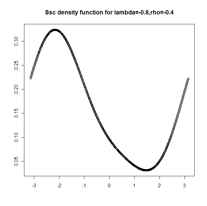
Figure 2. Ssc pdf for $\lambda=-0.8$ and $\rho=-0.4$

With theses values, if the practitioner concludes that $F\in D(H_{1})$, he is wrong in the use of the rule but his conclusion is correct by coincidence. So it is important to check the ultimate decreasingness of $F^{\prime}$, which is used in the proof of the rule.

3. Parameters estimation

3.1. Moments estimation

A. Point Estimation.

The $kth$ moment of $X$ is given by

$$\mathbb{E}X^{k}=\frac{1}{2\pi}\int_{-\pi}^{\pi}x^{k}(1+\lambda\sin x+\rho\cos x+(\lambda\rho/2)\sin 2x)\ dx.$$

From the following facts

$$\int_{-\pi}^{\pi}x\cos x\ dx=0,\ \ \int_{-\pi}^{\pi}x\sin x\ dx=2\pi,\ \ \int_{-\pi}^{\pi}x\cos x\sin x\ dx=-\pi/2$$

$$\int_{-\pi}^{\pi}x^{2}\cos x\ dx=-4\pi,\ \int_{-\pi}^{\pi}x^{2}\sin x\ dx=0,\ \ \int_{-\pi}^{\pi}x^{2}\sin x\cos x\ dx=0,$$

we get

$$m=\mathbb{E}X=\lambda(1-\rho/8),\ m_{2}=\mathbb{E}X^{2}=\pi^{2}/3-2\rho.$$

The moments estimators are solutions of the system of two equations : $m=\overline{X}_{n}$ and $m_{2}=m_{2,n}$. We immediately have, for $n\geq 1$,

(3.1) $$\hat{\rho}_{n}=(\pi^{2}/3-m_{2,n})/2\ and\ \hat{\lambda}_{n}=\frac{4\overline{X}_{n}}{4-\hat{\rho}_{n}}=\frac{8\overline{X}_{n}}{8-\pi^{2}/3+m_{2,n}}.$$

We may need to check such estimation by a simulation study. We will do this in Section 4 where we propose a simple method for generating data for the ssc distribution. For now we want to do more on the moment problem. In the appendix, we study the integrals, for $n\geq 0$,

$$I_{n}=\int_{-\pi}^{\pi}x^{n}\cos x\ dx,\ J_{n}=\int_{-\pi}^{\pi}x^{n}\sin x\ dx,\ and\ H_{n}=\int_{-\pi}^{\pi}x^{n}\sin 2x\ dx.\\$$

We established the following recurrence formula

(3.2) $$I_{0}=0,\forall n\geq 2,I_{2n}=-4n\pi^{2n-1}-2n(2n-1)I_{2(n-1)}\ and\ \forall n\geq 0,I_{2n+1}=0,,$$

(3.3) $$\forall n\geq 0,J_{2n}=0\ and\ \forall n\geq 1,J_{2n+1}=2\pi^{2n+1}-2n(2n+1)J_{2(n-1)+1},$$

and

(3.4) $$\forall n\geq 0,H_{2n}=0\ and\ \forall n\geq 1,H_{2n+1}=-\frac{\pi^{2n+1}}{2}-\frac{n(2n+1)H_{2(n-1)+1}}{2}.$$

and for the needs of that paper, we have computed

$$I_{1}=0,\ I_{2}=(2\pi)(-2\pi),\ I_{3}=0,\ I_{4}=4(2\pi)(6-\pi^{2}))$$

$$J_{1}=2\pi,\ J_{2}=0,\ J_{3}=(2\pi)(\pi^{2}-6),\ J_{4}=0$$

$$H_{1}=(2\pi)(-1/4),\ H_{2}=0,H_{3}=(2\pi)((3-2\pi^{2})/8),\ H_{4}=0.$$

With such facts, we easily have

$$\mathbb{E}X^{3} = \lambda(\pi^{2}-6)+\frac{\lambda\rho}{8}(3-2\pi^{2})$$

(3.5) $$\mathbb{E}X^{4} = \frac{\pi^{4}}{5}-4\rho(\pi^{2}-6).$$

We will see how we need these parameters for the asymptotic laws of the moment estimators.

4. The characteristic function

Proposition 1.

The characteristic function (fc) of $X$ is given, for $t\notin\{-2,-1,0,1,2\}$, bt

$$\psi(t)=\frac{1}{\pi}\left(\frac{1}{t}+\frac{\lambda}{i(t^{2}-1)}-\frac{\rho t}{t^{2}-1}-\frac{\lambda\rho}{i(t^{2}-4)}\right)sin(\pi t)$$

and is extended to values in $\{-2,-1,0,1,2\}$ by continuity of the fc.

Proof. We may write for $t\in\mathbb{R}$ and $x\in[-\pi,\pi]$,

$$e^{it}f(x) = \frac{1}{2\pi}e^{itx}\left[1+\frac{\lambda}{2i}\left(e^{ix}-e^{-ix}\right)+\frac{\rho}{2}\left(e^{ix}+e^{-ix}\right)+\frac{\lambda\rho}{4}\left(e^{i2x}-e^{-i2x}\right)\right]$$

$$= \frac{1}{2\pi}\left[e^{itx}+\frac{\lambda}{2i}\left(e^{ix(t+1)}-e^{ix(t-1)}\right)+\frac{\rho}{2}\left(e^{ix(t+1)}+e^{ix(t-1)}\right)\right.$$

$$+ \left.\frac{\lambda\rho}{4}\left(e^{ix(t+2)}-e^{-ix(t-2)}\right)\right].$$

Integrating from $-\pi$ to $+\pi$ leads to the announced results. $\square$

B. Asymptotic Normality of the moment estimators and Statistical tests.

The moments estimators are treated by using the function empirical process defined, for any $n\geq 1$ and $h\in L^{2}(\mathbb{P}_{X})$, by

$$\mathbb{G}_{n}(h)=\frac{1}{\sqrt{n}}\sum_{j=1}^{n}(h(X_{j})-\mathbb{E}(h(X_{j}))),$$

as explained in Lo (2016) and Lo (2018a). For a more general source, the book by van der Vaart and Wellner (1996) is one the best in the field but we no need the great artillery provided there. We have the following result.

Theorem 3.

we have the asymptotic laws of the moment estimators, as $n\rightarrow+\infty$,

$$\left(\sqrt{n}(\hat{\rho}_{n}-\rho),\sqrt{n}(\hat{\lambda}_{n}-\lambda)\right)\rightsquigarrow\mathcal{N}_{2}\left(0,\Sigma\right),$$

with

$$\Sigma_{11}=\frac{\mathbb{V}ar(X^{2})}{4},\ \ \Sigma_{11}=\frac{\mathbb{V}ar(X+\lambda X^{2})}{\mu^{2}}$$

and

$$\Sigma_{12}=\Sigma_{21}=-\frac{\mathbb{C}ov(X^{2},X+\lambda X^{2})}{2\mu}.$$

Remark. As anticipated in Formula 3.5, the asymptotic laws need the first four moments of $X$.

Proof. Let us set $h_{\ell}(x)=x^{\ell}$ for $x\in\mathbb{R}$. By applying the methods in Lo (2016), we get

$$\sqrt{n}(\hat{\rho}_{n}-\rho)=\mathbb{G}_{n}(-h_{2}/2)+o_{\mathbb{P}(1)}.$$

Next, we have

$$\hat{\lambda}_{n}=\frac{8\left(m+\frac{1}{\sqrt{n}}\mathbb{G}_{n}(h_{1})\right)}{8-\pi^{2}/3+m_{2}+\frac{1}{\sqrt{n}}\mathbb{G}_{n}(h_{2})}.$$

By Lemma 2 in Lo (2016), we get that for $\mu=8-\pi^{2}/3+m_{2}$,

$$\sqrt{n}(\hat{\lambda}_{n}-\lambda)=\mathbb{G}_{n}((h_{1}+\lambda h_{2})/\mu)+o_{\mathbb{P}(1)}.$$

By using the functional Brownian stochastic process $\mathbb{G}$, which is the weak limit of $\mathbb{G}_{n}$ and defined by the variance-covariance function

$$\Gamma(h,k)=\int_{\mathbb{R}}(h(x)-\mathbb{E}h(X))(k(x)-\mathbb{E}k(X))d\mathbb{P}_{X}(x),$$

where $(h,k)\in L^{2}(\mathbb{P}_{X})^{2}$, we get that

$$\left(\sqrt{n}(\hat{\rho}_{n}-\rho),\sqrt{n}(\hat{\lambda}_{n}-\lambda)\right)\rightsquigarrow\mathcal{N}_{2}\left(0,\Sigma\right),$$

with

$$\Sigma_{11}=\frac{\mathbb{V}ar(h_{2}(X^{2})}{4},\ \ \Sigma_{11}=\frac{\mathbb{V}ar(h_{1}(X)+\lambda h_{2}(X)}{\mu^{2}}$$

and

$$\Sigma_{12}=\Sigma_{21}=-\frac{\mathbb{C}ov(h_{2}(X),h_{1}(X)+\lambda h_{2}(X))}{2\mu}.\ \blacksquare$$

4.1. Maximum Likelihood Estimators

we are going to see that the ML-estimators are not defined here. We begin the remark that the first three linear differential operators in $(\lambda,\rho)$ of $f$ are

$$2\pi Df(u,v)=\sin x(1+\rho\cos x)u+\cos x(1+\lambda\sin x)v,$$

$$2\pi D^{2}f(u,v)=(\cos x\sin x)uv,\ (u,v)\in\mathbb{R},$$

$$D^{3}f(u,v)=0.$$

By applying the Taylor-Lagrange-Cauchy formula (see Valiron (1946), page 233) : for $(\lambda,\lambda_{0},\rho,\rho_{0})\in[-1,1]^{4}$, for $|\theta_{i}|<1$, $i=1,2$

$$f(x,\lambda,\rho) = f(x,\lambda_{0},\rho_{0})+Df(\lambda-\lambda_{0},\rho-\rho_{0})+\frac{1}{2}D^{2}f(\lambda-\lambda_{0},\rho-\rho_{0})$$

$$+ D^{2}f(\theta_{1}(\lambda-\lambda_{0}),\theta_{2}(\rho-\rho_{0})),$$

and we get

$$f(x,\lambda,\rho) = f(x,\lambda_{0},\rho_{0})+\sin x(1+\rho\cos x)(\lambda-\lambda_{0})+\cos x(1+\lambda\sin x)(\rho-\rho_{0})$$

$$+ (\cos x\sin x)(\lambda-\lambda_{0})(\rho-\rho_{0})$$

First, for $x\notin\{\mp\pi,\pm\pi/2\}$, the zeros of $f$ are $-1/\sin x$ and $-1/\cos x$ which do not belong to $[-1,1]$. Even on $\mathbb{R}$, not requiring that $f$ be non-negative to make it a probability density function, Formula which becomes at any critical point $(\lambda_{0},\rho_{0})$ of this $C^{1}$-function (in $\lambda$ and in $\rho$),

$$f(x,\lambda,\rho) = (\cos x\sin x)(\lambda-\lambda_{0})(\rho-\rho_{0}).$$

So, for a fixed $x\notin\{\mp\pi,\pm\pi/2\}$, there can be an extremum point $(\lambda_{0},\rho_{0})$ for the likelihood function.

5. Generation

Since the cdf $F$ is explicitly known and is strictly increasing and continuous, we may use the dichotomous algorithm to find the inverse of $F$. It works as follows. Given $v\in[0,1]$, to find $x$ such that $F(x)=v$, we fix the number of decimals of the solution $x$ denoted nbrDec. In the Appendix, beginning by page References, the VB 6 code for computing the cdf $F$ is given in page References, the Dichotomous algorithm is described in page References and implemented in VB6 in References. Finally, the VB 6 subroutine which generates a sample of an arbitrary size is given in References.

A. Numerical test of the computer programs.

For different values for $\lambda$ and $\rho$ in $]-1,1[$, samples of size $n=1000$ are generated and the comparison between the exact means and the second moments as given in Formua are compared with the sample counterparts. Table 1 demonstrates the quality of the generation.

$\lambda$	$\rho$	mean (E)	mean (M)	2nd moment (E)	2nd moment (M)	quotient (Q)
0.9	-0.9	1.1025	1.2322	5.0898	5.0281	1.0122
0.9	-0.6	1.035	1.0641	4.4898	4.4796	1.0022
0.9	-0.3	0.9675	0.9396	3.8898	3.8987	0.9977
0.9	0.1	0.8775	0.8796	3.0898	3.2221	0.9589
0.9	0.4	0.81	0.8048	2.4898	2.5953	0.9593
0.9	0.7	0.7425	0.7536	1.8898	1.8690	1.0111
0.9	0.9	0.6975	0.7077	1.4898	1.4810	1.0059
-0.9	0.9	-0.6975	-0.6972	1.4898	1.5574	0.9566
-0.9	0.7	-0.7425	-0.7773	1.8898	1.8280	1.0338
-0.9	0.4	-0.81	-0.8218	2.4898	2.2965	1.0841
-0.9	0.1	-0.8775	-0.9273	3.0898	3.2964	0.9373
-0.9	-0.3	-0.9675	-1.0273	3.8898	3.9613	0.9819
-0.9	-0.6	-1.035	-0.9654	4.4898	4.4845	1.0011
-0.9	-0.9	-1.1025	-1.1300	5.0898	5.1902	0.9806

Table 1. Legend : (E) : Exact, (M) empirical, (Q) : quotient exact second moment to empirical second moment

B. Moment estimation.

Based on the generation techniques as introduced above, we also report interesting performances for the estimation of the parameter when the sizes varies in Table 2. The Mean Absolute Error (MAE) and the Mean Square-root Quadratic Error (MSQE) are reported both for $\lambda$ and $\rho$. These simulations have been for $\lambda=\rho=-0.9$.

Error n	10	50	100	200	300	400	500	750	1000
MAE-$\lambda$	41.17	18.44	11.88	10.41	7.39	5.93	5.43	5.08	3.91
SMQE-$\lambda$	51.97	22.49	15.04	12.07	9.81	7.74	6.78	6.17	5.20
MAE-$\rho$	29.83	15.20	10.05	8.51	4.97	5.56	4.59	3.56	3.14
SMQE-$\rho$	37.44	18.10	13.10	10.09	6.49	7.17	5.66	4.41	2.89

Table 2. Errors given in $100$ multiples

Figure 3 shows how both errors decreases to zero.

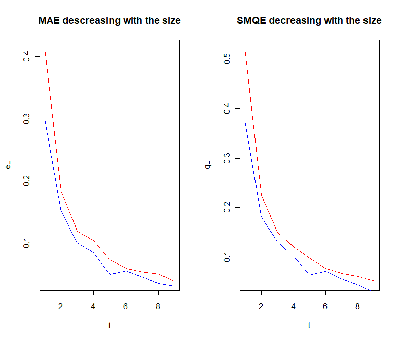
Figure 3. Red : related to $\rho$. Blue : errors related to $\rho$

6. Conclusion

This is an immediate contribution of the study of the Sine Skewed Caedioid distribution. Further deeper properties will be addressed later.

Appendix.

I. Integral Computations.

Let us define, for $n\geq 0$,

$$I_{n}=\int_{-\pi}^{\pi}x^{n}\cos x\ dx,\ \int_{-\pi}^{\pi}x^{n}\sin x\ dx,\ \int_{-\pi}^{\pi}x^{n}\cos 2x\ dx\ and\ \int_{-\pi}^{\pi}x^{n}\sin 2x\ dx.\\$$

A - Computation of $I_{n}$. For $n=0$,

$$I_{0}=\int_{-\pi}^{\pi}\cos x\ dx=\int_{-\pi}^{\pi}d(\sin x)=0$$

and for $n=1$,

$$I_{1}=\int_{-\pi}^{\pi}xd(\sin x)=[x\sin x]^{-\pi}_{\pi}-\int_{-\pi}^{\pi}-d(\cos x)=0$$

and for $n=2$

$$I_{2} = \int_{-\pi}^{\pi}x^{2}d(\sin x)=]x^{2}\sin x[^{-\pi}_{\pi}-2\int_{-\pi}^{\pi}-2xd(\cos x)$$

$$= \left(4[x\cos x]^{-\pi}_{\pi}-\int_{-\pi}^{\pi}\cos x)\right)$$

$$= 4[x\cos x]^{-\pi}_{\pi}=-4\pi.$$

Now, the general guess is that $I_{2n+1}=0$ for $n\geq 0$. Since this already holds $n=0$, let us remark that for $n\geq 1$,

$$I_{2n+1} = \int_{-\pi}^{\pi}x^{2n+1}d(\sin x)=]x^{2n+1}\sin x[^{-\pi}_{\pi}-(2n+1)\int_{-\pi}^{\pi}-x^{2n}d(\cos x)$$

$$= (2n+1)\int_{-\pi}^{\pi}x^{2n}d(\cos x)=(2n+1)[x^{2n}\cos x]^{-\pi}_{\pi}-(2n)(2n+1)\int_{-\pi}^{\pi}-x^{2n-1}\cos x\ dx$$

$$= -(2n)(2n+1)I_{2(n-1)+1}.$$

By an descendent induction, we will have $I_{2n+1}=C_{n}I_{1}=0$. Now, we have to find $I_{2n}$, for $n\geq 1$, which is

$$I_{2n} = \int_{-\pi}^{\pi}x^{2n}d(\sin x)=]x^{2n}\sin x[^{-\pi}_{\pi}-(2n)\int_{-\pi}^{\pi}(-x^{2n-1})d(\cos x)$$

$$= (2n)\int_{-\pi}^{\pi}x^{2n-1}d(\cos x)=[x^{2n-1}\cos x]^{-\pi}_{\pi}-(2n)(2n-1)\int_{-\pi}^{\pi}-x^{2(n-1)}\cos x\ dx$$

$$= -4n\pi^{2n-1}-2n(2n-1)I_{2(n-1)}.$$

For example, we find again $I_{2}=-4\pi$ for $n=1$.

B - Computation of $J_{n}$. For $n=0$, we have

$$J_{0}=\int_{-\pi}^{\pi}\sin x\ dx=\int_{-\pi}^{\pi}d(-\cos x)=0$$

and for $n=1$,

$$J_{1}=\int_{-\pi}^{\pi}xd(-\cos x)=-[x\cos x]^{-\pi}_{\pi}+\int_{-\pi}^{\pi}-d(\sin x)=2\pi.$$

Our guess is that $J_{2n}=0$ for $n\geq 0$ and we have for $n\geq 1$,

$$J_{2n} = \int_{-\pi}^{\pi}x^{2n}d(-\cos x)=]x^{2n}\cos x[^{-\pi}_{\pi}+(2n)\int_{-\pi}^{\pi}x^{2n-1}d(\sin x)$$

$$= (2n)\int_{-\pi}^{\pi}x^{2n-1}d(\sin x)=(2n)[x^{2n-1}\sin x]^{-\pi}_{\pi}-(2n)(2n-1)\int_{-\pi}^{\pi}x^{2(n-1)}\sin x\ dx$$

$$= -(2n)(2n-1)J_{(n-1)}.$$

By an descendent induction, we will have $J_{2n}=C_{n}J_{0}=0$. Now, he have to find $J_{2n+1}$, for $n\geq 1$, which is

$$J_{2n+1} = \int_{-\pi}^{\pi}x^{2n+1}d(-\cos x)=-]x^{2n+1}\cos x[^{-\pi}_{\pi}+(2n+1)\int_{-\pi}^{\pi}x^{2n}d(\sin x)$$

$$= 2\pi^{2n+1}+(2n+1)[x^{2n}\sin x]^{-\pi}_{\pi}-(2n)(2n+1)\int_{-\pi}^{\pi}x^{2(n-1)+1}\sin x\ dx$$

$$= 2\pi^{2n+1}-2n(2n+1)J_{2(n-1)+1}.$$

C - Computation of $H_{n}$. For $n=0$, we have

$$H_{0}=\int_{-\pi}^{\pi}\sin xd(\sin x)=(1/2)\int_{-\pi}^{\pi}d(\sin^{2}x)=0,$$

and for $n=1$,

$$H_{1} = (1/2)\int_{-\pi}^{\pi}x\sin 2x\ dx=-(1/4)\int_{-\pi}^{\pi}xd(\cos 2x)$$

$$= -(1/4)\left([x\cos 2x]^{-\pi}_{\pi}-\int_{-\pi}^{\pi}(1/2)d(\sin 2x)\right)$$

$$= -\pi/2.$$

We still guess that $H_{2n}=0$ for $n\geq 0$ and find, for $n\geq 0$,

$$H_{2n} = (1/2)\int_{-\pi}^{\pi}x^{2n}\sin 2x\ dx=-(1/4)\int_{-\pi}^{\pi}x^{2n}d(\cos 2x)$$

$$= -(1/4)\left([x^{2n}\cos 2x]^{-\pi}_{\pi}-(1/2)(2n)\int_{-\pi}^{\pi}x^{2n-1}d(\sin 2x)\right)$$

$$= (1/4)n\int_{-\pi}^{\pi}x^{2n-1}d(\sin 2x)=(1/4)n\left([x^{2n-1}\sin 2x]^{-\pi}_{\pi}-(2n-1)\int_{-\pi}^{\pi}x^{2(n-1)}\sin 2x\ dx\right)$$

$$= -(1/4)n(2n-1)H_{2(n-1)},$$

and we conclude that $H_{2n}=0$ for all $n\geq 0$, based on that $H_{0}=0$ and the unveiled descendent induction formula above. Nor for all $n\geq 0$,

$$H_{2n+1} = (1/2)\int_{-\pi}^{\pi}x^{2n+1}\sin 2x\ dx=-(1/4)\int_{-\pi}^{\pi}x^{2n+1}d(\cos 2x)$$

$$= -(1/4)\left([x^{2n+1}\cos 2x]^{-\pi}_{\pi}-(1/2)(2n+1)\int_{-\pi}^{\pi}x^{2n}d(\sin 2x)\right)$$

$$= -(1/4)\left((2\pi^{2n+1})-(1/2)(2n+1)\left([x^{2n}\sin 2x]^{-\pi}_{\pi}-(2n)\int_{-\pi}^{\pi}x^{2n-1}\sin 2x)\right)\right)$$

$$= -(1/2)\pi^{2n+1}-(1/4)(1/2)(2n+1)(2n)\int_{-\pi}^{\pi}x^{2n-1}\sin 2x)$$

$$= -(1/2)\pi^{2n+1}-(1/2)n(2n+1)H_{2(n-1)+1}$$

We conclude

(6.1) $$I_{0}=0,\forall n\geq 2,I_{2n}=-4n\pi^{2n-1}-2n(2n-1)I_{2(n-1)}\ and\ \forall n\geq 0,I_{2n+1}=0,,$$

(6.2) $$\forall n\geq 0,J_{2n}=0\ and\ \forall n\geq 1,J_{2n+1}=2\pi^{2n+1}-2n(2n+1)J_{2(n-1)+1},$$

and

(6.3) $$\forall n\geq 0,H_{2n}=0\ and\ \forall n\geq 1,H_{2n+1}=-\frac{\pi^{2n+1}}{2}-\frac{n(2n+1)H_{2(n-1)+1}}{2}.$$

For the needs of this paper, we have

$$I_{1}=0,\ I_{2}=(2\pi)(-2\pi),\ I_{3}=0,\ I_{4}=4(2\pi)(6-\pi^{2}),$$

$$\ I_{5}=0,\ I_{6}=-6(2\pi)(\pi^{4}-20\pi^{2}+120),\ I_{7}=0,\ I_{8}=-8(2\pi)(\pi^{6}-42\pi^{4}+840\pi^{2}-5040)$$

$$J_{1}=2\pi,\ J_{2}=0,\ J_{3}=(2\pi)(\pi^{2}-6),\ J_{4}=0,$$

$$J_{5}=2\pi(\pi^{4}-20\pi^{2}+120),\ J_{6}=0,\ J_{7}=2\pi(\pi^{6}-42\pi^{4}+840\pi^{2}-5040),\ J_{8}=0,$$

$$H_{1}=(2\pi)(-1/4),\ H_{2}=0,H_{3}=(2\pi)((3-2\pi^{2})/8),\ H_{0}=0,$$

$$H_{5}=-2\pi\frac{(2\pi^{4}-10\pi^{2}+15)}{8},\ H_{6}=0,\ H_{7}=-2\pi\frac{(4\pi^{6}-42\pi^{4}+210\pi^{2}-315)}{16}.$$

$$\mathbb{E}X^{5} = \lambda(\pi^{4}-20\pi^{2}+120)-\frac{\lambda\rho}{16}(2\pi^{4}-10\pi^{2}+15)$$

$$\mathbb{E}X^{6} = \frac{\pi^{6}}{7}-6\rho(\pi^{4}-20\pi^{2}+120)$$

$$\mathbb{E}X^{7} = \lambda(\pi^{6}-42\pi^{4}+840\pi^{2}-5040)-\frac{\lambda\rho}{32}(4\pi^{6}-42\pi^{4}+210\pi^{2}+315)$$

$$\mathbb{E}X^{8} = \frac{\pi^{8}}{9}-8\rho(\pi^{6}-42\pi^{4}+840\pi^{2}-5040).$$

II. Samples generations.

Description of the dichotomous algorithm.

⬇

0. Fix the count index of the decimals countDec to -1 : countDec=-1.

1. Fix x=1 and compute F(1).

2. IF F(1)=v. Take x=1. Stop

3. IF F(1)<v, then

3a. Fix x=1 and set h=1.

3b. Progressively increment x by h and test

and compare F(x) and v.

3bA. IF F(x)=v. x is the searched number.Stop

3bB. IF F(x)<v, Goto 3bA and continue

the incrementation.

3bC. IF F(x)>v, then

Decrement by h : x=x-h

Increment countDec

If countDec<nbrDec

take h=h/10

Goto 3b

If countDec=nbrDec. Stop

3. IF F(1)>v, then

4a. Fix x=1 and set h=0.1

4b. Progressively decrement x by h : x=x-h and test and compare

F(x) and v.

4bA. IF F(x)=v. x is the searched number.Stop

4bB. IF F(x)>v, Goto 4bA and continue

the decrementation

4bC. IF F(x)<v, then

increment by h : x=x-h

Increment countDec

If countDec<nbrDec-1

take h=h/10

Goto 4b

If countDec=nbrDec. Stop

Implementation of the dichotomous algorithm in Visual Basic 6.

⬇

Function sscinv(v As Double, lambda As Double, rho As Double, nbrDec) As Double

Dim dich As Double, count As Integer, h As Double

Dim countDec

sscinv = 1

dich = ssc(sscinv, lambda, rho)

If (dich = v) Then

Exit Function

End If

If (dich < v) Then

h = 1

count = 0

countDec = -1

While ((countDec < nbrDec) And (count < 2000))

count = count + 1

sscinv = sscinv + h

If (ssc(sscinv, lambda, rho) = v) Then

Exit Function

End If

If (ssc(sscinv, lambda, rho) > v) Then

countDec = countDec + 1

sscinv = sscinv - h

h = h / 10

End If

Wend

End If

If (dich > v) Then

h = 0.1

count = 0

countDec = 0

While ((countDec < nbrDec) And (count < 2000))

count = count + 1

sscinv = sscinv - h

If (ssc(sscinv, lambda, rho) = v) Then

Exit Function

End If

If (ssc(sscinv, lambda, rho) < v) Then

countDec = countDec + 1

sscinv = sscinv + h

h = h / 10

End If

Wend

End If

End Function

VB6 Subroutine for cumputing the cdf $F$.

⬇

Private Function ssc(x As Double, lambda As Double, rho As Double) As Double

Dim pi As Double

pi = 4 * Atn(1)

ssc = (1 / 2) + (1 / (2 * pi)) * (x - (lambda * (Cos(x) + 1)) + rho * Sin(x)

- (((lambda * rho) / 4) * (Cos(2 * x) - 1)))

End Function

rssc : VB6 Subroutine for generating samples from the ssc distribution, which the sample in the file ssc100.

⬇

Sub rssc(tail As Integer, lambda As Double, rho As Double, nbrDec As Integer)

Dim ii As Integer, cheminD As String

cheminD = ”G:\backup\DataGslo\gslo\TveSimulation\ssc\”

Open cheminD & ”ssc100.txt” For Output As #1

Randomize Timer

For ii = 1 To tail

Print #1, sscinv(Rnd(1), lambda, rho, nbrDec)

Next

Close #1

End Sub

References

• Ahsanullah (2018) Ahsanullah M. (2018). Sine-Skewed Cardioid Distribution. In A Collection of Papers in Mathematics and Related Sciences, a festschrift in honour of the late Galaye Dia (Editors : Seydi H., Lo G.S. and Diakhaby A.). Spas Editions, Euclid Series Book. To appear
• Lo (2018a) Lo G.S.(2018). Weak Convergence (IIIA) - A handbook of Asymptotic Representations of Statistics in the Functional Empirical process and Applications. Arxiv :
• Lo (2016) Lo G.S.(2016). How to use the functional empirical process for deriving asymptotic laws for functions of the sample. ArXiv:1607.02745.
• Lo (2018b) Lo G.S.(2018). Weak Convergence (IIA) - Functional and Random Aspects of Univariate Theory of Extreme Value Theory. Arxiv : 1810.01625.
• Valiron (1946) Valiron, G.(1946). Théorie des Functions. Masson. Paris.
• van der Vaart and Wellner (1996) van der Vaart A. W. and Wellner J. A.(1996). Weak Convergence and Empirical Processes With Applications to Statistics. Springer, New-York.