Vacancy-induced Fano resonances in zigzag phosphorene nanoribbons

Abstract

Motivated by recent scanning tunneling microscopy/spectroscopy experiments on probing single vacancies in black phosphorus, we present a theory for Fano antiresonances induced by coupling between vacancy states and edge states of zigzag phosphorene nanoribbons (zPNRs). To this end, in the first step, using the tight-binding Hamiltonian, we obtain an analytic solution on the lattice for the state associated to a single vacancy located in the bulk phosphorene which shows a highly anisotropic localization in real space. For a finite zigzag ribbon, in the absence of particle-hole symmetry, the localized state induced by vacancies can couple to the wave functions of the edge states which results in the formation of a new bound state. The energy of vacancy bound state lies inside the quasi-flat band composed of edge states when the vacancy locates sufficiently far away from the edge. Then, we employ the T-matrix Lippmann-Schwinger approach to obtain an explicit analytical expression for the scattering amplitude of the edge electrons of a zPNR by the presence of a single vacancy which shows a Fano resonance profile with a tunable dip. We demonstrate that varying the position of the vacancy produces substantially different effects on the resonance width, resonance energy position, and the asymmetry parameter of Fano line shape. Furthermore, the validity of the theoretical descriptions is verified numerically by using the Landauer approach.

I Introduction 

The existence of great transport properties and potential applications of a new semiconducting material, called black phosphorus (BP), has attracted a lot of attention recently Li2014 ; Li2016 ; Liu2014 ; Xia2014 ; Neto-2014 ; Ling2015 . BP has a layered structure with van der Waals interaction between individual atomic layers and it is possible to exfoliate a single atomic layer from its bulk which is called phosphorene Li2014 ; Liu2014 . In this new specimen of two-dimensional (2D) material, each phosphorus atom is covalently bonded with three nearest neighbors via $sp^{3}$ hybridization to form a puckered 2D honeycomb structure. This unique property of anisotropy on one hand, and a tunable and large direct band gap, on the other hand, makes phosphorene a desirable candidate material for different applications with specific electronic, mechanical, thermal, and transport features Carvalho2016 ; Neto2014 ; Qiao2014 ; Peeters2014 ; Guinea2014 ; Yang2014 ; Katsnelson2015 . Furthermore, confining one of the dimensions of phosphorene to a ribbon with the zigzag edge which is called zigzag phosphorene nanoribbon introduces degenerate quasi-flat bands in the middle of the gap detached entirely from the valence and conduction bands Ezawa2014 ; Peeters-skew . Due to the presence of such edge modes, the quantum transport properties of zPNRs resembles a quasi-one-dimensional (Q1D) system in this energy window Ezawa2014 ; Asgari2018 ; Amini2018 .

Despite the vast literature regarding different theoretical and experimental researches on perfect PNRs as mentioned above, the body of work dedicated to their defective counterparts is surprisingly small. For instance, the electronic band structure of defective phosphorene, as well as the formation energy of atomic vacancies, are studied numerically in Ref. Hu2015 ; Wang2015 . But among these studies, there is an experiment carried out recently Katsnelson2017 which is the observation of atomic vacancies on the surface of bulk BP. The spatial distribution of wave function amplitudes around a vacancy which is observed by scanning tunneling microscopy tomographic imaging exhibits strong anisotropy. Another significant aspect of the presence of vacancies is their effects on quantum transport through the edges of the zPNRs which is computed numerically in Ref. Peeters2018 using the tight-binding approach. It is found that single vacancies can create quasi-localized states which can affect the transport properties of zPNRs by introducing antiresonant dips in the edge conductance of the ribbons.

However, the results outlined in the previous paragraph bring up an important question of whether the conductance dips computed for the electronic transmission through the edges of zPNR is due to the coupling of anisotropic vacancy state to the continuum states of the edges resulting in the so-called Fano antiresonance in the wave propagation. Indeed, Fano resonance Fano is one of the most important resonance mechanisms in which a discrete level couples to an energetically close-by continuum of states giving rise to new scattering paths. It is quite predictable that a single vacancy can introduce a new localized state within the energy window of the edge modes. Therefore, a possible scenario to understand the corresponding conductance dips of vacant zPNRs can be due to the coupling of the edge states forming a quasi-flat band to the vacancy wave function. In this work, we present the theory of such resonance scattering due to the vacancy defect leading to Fano resonance in the transmission of edge channels in zPNRs. To this end, we first use a tight-binding model to obtain and analyze in detail the localized state induced by a vacancy defect in the energy interval of the edge band in zPNRs. Then, we employ the general scattering theory based on the Green’s function approach and the Lippmann-Schwinger equation to investigate the antiresonance dips in the electronic transmission through the edge states of zPNRs due to the presence of such a localized state.

The paper is organized as follows. In section II, we provide the rigorous derivation of localized wave function around a single vacancy in phosphorene using the tight-binding Hamiltonian. In this section, the energy shift of such a bound state due to the absence of electron-hole symmetry is explained. In section III, we generally introduce the theory of a Fano antiresonance induced by the coupling of an impurity state to a continuum of states using the T-matrix Lippmann-Schwinger approach. We employ this formalism in section IV to obtain the Fano antiresonance dips in the electronic transmission through the edge states of zPNR which is induced by a single vacancy near the edge. Section V is devoted to discussion on the obtained results and, finally, we wrap up the paper with the summary and concluding remarks in section VI.

II Localized states around vacancies in bulk phosphorene

Phosphorene consists of a non-planar puckered honeycomb lattice of phosphorus atoms with two in-equivalent sublattices denoted by $A$ and $B$ as shown in Fig. 1. We choose the $x$ and $y$ axes along the zigzag and armchair chains respectively. Now, it is possible to describe each lattice site by $(m,n,\nu)$ where $m$ and $n$ are armchair and zigzag chain numbers respectively and $\nu=A,B$. The energy band structure of phosphorene can be well described using a tight-binding model Ezawa2014 ; Rudenko2014

$${{\widehat{H}}}=\sum_{\langle i,j\rangle}t_{ij}c_{i}^{\dagger}c_{j}+h.c.,$$ (1)

where $\langle i,j\rangle$ represents summation over only considered neighbors. Here, $t_{ij}$ is the hopping energy between sites $i$ and $j$, $c^{\dagger}_{i}(c_{i})$ is the electron creation (annihilation) operator in site $i$, and $h.c.$ stands for hermitian conjugate. It is shown that considering only five hopping integrals $t_{1}=-1.220$ eV, $t_{2}=3.665$ eV, $t_{3}=-0.205$ eV, $t_{4}=-0.105$ eV, and $t_{5}=-0.055$ eV in this model, which is shown in Fig. 1, provides a reasonable description of the phosphorene band structure Rudenko2014 . However, for analytical calculations, it is reasonable to neglect hopping terms $t_{3}$ and $t_{5}$ which have a smaller contribution to the Hamiltonian in comparison to $t_{1}$ and $t_{2}$ terms. It is important to note that the presence of $t_{4}$ breaks both electron-hole and lattice inversion symmetries of phosphorene and we will take into account its effect perturbatively later. Therefore, we can rewrite the above Hamiltonian keeping only the important terms of first, second and fourth nearest neighbors as

$$\begin{split}{{\widehat{H}}}&={{\widehat{H}}_{0}}+{{\widehat{H}}_{1}},\\ {{\widehat{H}}_{0}}&=t_{1}\sum_{\langle i,j\rangle_{\text{1st}}}c_{i}^{\dagger}c_{j}+t_{2}\sum_{\langle i,j\rangle_{\text{2nd}}}c_{i}^{\dagger}c_{j}+h.c.,\\ {{\widehat{H}}_{1}}&=t_{4}\sum_{\langle i,j\rangle_{\text{4th}}}c_{i}^{\dagger}c_{j}+h.c.\end{split}$$ (2)

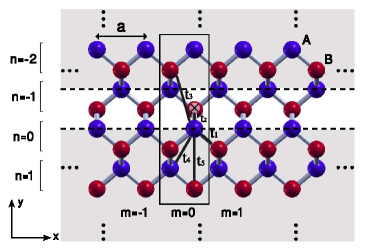
Figure 1: (Color online). Schematic view of the lattice structure of phosphorene in real space. The lattice constant is $a$, $m$ is the index of the vertical armchair chain along the horizontal direction and $n$ labels the horizontal zigzag chain along the vertical direction. This lattice consists of two different types of sublattices denoted by $A$ and $B$ and a single vacancy which is located on site $(m=0,n=-1,B)$ and denoted by $\times$ symbol.

Without loss of any generality, let us now consider a single vacancy placed at site $(0,-1,B)$. This is equivalent to turning the hopping terms that connect this site to its neighbors off. In the presence of particle-hole symmetry, $t_{4}=0$, this implies the appearance of a new zero energy state which has only non-zero amplitudes on the $A$ sublattice Pereira2008 and we call it $|\Psi_{v}^{A}\rangle$. Therefore, it should satisfy the condition

$${\widehat{H}_{0}}|\Psi_{v}^{A}\rangle=0.$$ (3)

Later, we will calculate the effect of $t_{4}$ perturbatively which shifts this energy toward the negative values.

Indeed, a single vacancy can divide the phosphorene plane into an upper semi-infinite ribbon with beard edge and a lower one with the zigzag edge which is shown by black dashed lines in Fig. 1. The upper semi-infinite ribbon with beard edge does not support localized edge states Ezawa2014 . So, the vacancy wave function amplitudes are zero in the upper half-plane. On the other hand, due to the absence of hopping between site $(0,0,A)$ and the vacant site, a possible solution in the lower half-plane can start with non-zero amplitude on this site, namely $\langle 0,0,A|\Psi_{v}^{A}\rangle\neq 0$. Also Eq. (3) implies that $t_{2}\langle 1,1,A|\Psi_{v}^{A}\rangle+t_{1}\langle 0,0,A|\Psi_{v}^{A}\rangle=0$ which results in $\langle 1,1,A|\Psi_{v}^{A}\rangle=(-t_{2}/t_{1})\langle 0,0,A|\Psi_{v}^{A}\rangle$. With the same kind of reasoning it is evident that $\langle 0,1,A|\Psi_{v}^{A}\rangle=(-t_{2}/t_{1})\langle 0,0,A|\Psi_{v}^{A}\rangle$. Next, one can apply the same procedure to obtain the amplitudes of the wave function on the next zigzag chains which we do not pursue it here. Instead, we focus on a more systematic way of constructing the vacancy wave function  Pereira2006 ; Vozmediano below.

Let us consider the lower semi-infinite zigzag ribbon in which the amplitudes of the vacancy wave function is non-zero. The typical edge states of this ribbon have the following wave functions Amini2018

$$|\Psi^{A}(k)\rangle=\frac{1}{\sqrt{\pi}}\sum_{m,n}\alpha^{n}(k)\gamma(k)e^{ik(m-\delta_{n})}|m,n,A\rangle,$$ (4)

where $k$ is the wave vector measured in units of $1/a$ (and $a$ is the lattice constant) along the horizontal axis. Here, $\delta_{n}$ is a constant value equal to 0 (0.5) for even (odd) $n$, $\alpha(k)=-2(t_{1}/t_{2})\cos{(k/2)}$, and $\gamma(k)=\sqrt{1-\alpha^{2}(k)}$. Also, the superscript $A$ denotes the type of sublattice in which the wave function is localized and $n$ is the zigzag chain number measured from the edge (starting from zero). Therefore, the idea is to express the zero energy vacancy state as a superposition of these edge states with zero components everywhere along the zigzag edge except on site $(0,0,A)$. The following combination of the edge states can satisfy such a condition

$$|\Psi_{v}^{A}\rangle=c\int_{-\pi}^{\pi}\gamma^{-1}({k})|\Psi^{A}(k)\rangle dk,$$ (5)

in which $c$ is the normalization coefficient given by

$$c^{-2}=\int_{-\pi}^{\pi}\gamma^{-2}(k)dk.$$ (6)

Now, we can obtain the amplitudes of the wave function in Eq. (5) on different lattice sites. Let us start from

$$\begin{split}\langle m,0,A|\Psi_{v}^{A}\rangle&=c\int_{-\pi}^{\pi}\gamma^{-1}(k)\langle m,0,A|\Psi^{A}(k)\rangle dk\\ &=c\int_{-\pi}^{\pi}e^{ikm}dk=c\delta_{m,0}.\end{split}$$ (7)

This ensures our desired form of the wave function on the $n=0$ zigzag chain. Clearly, we can go on and calculate the wave function amplitudes on the $n=1$ zigzag chain as

$$\begin{split}\langle m,1,A|\Psi_{v}^{A}\rangle&=c\int_{-\pi}^{\pi}\gamma^{-1}(k)\langle m,1,A|\Psi^{A}(k)\rangle dk\\ &=c\int_{-\pi}^{\pi}dk\cos{(k/2)}\left[e^{ik(m-1/2)}+e^{-ik(m+1/2)}\right]\\ &=(-t_{2}/t_{1})c\left[\delta_{m,0}+\delta_{m-1,0}\right].\end{split}$$ (8)

This is equivalent to the results of the first method which we described before. Fig. 2 represents the corresponding wave function amplitudes around a vacancy located on the site which is denoted by $\times$ symbol. As it is shown, the vacancy wave function is highly anisotropic and non-zero in a region like a triangle over the apposite sublattice in which the vacancy is located. This vacancy wave function resembles the topological boundary state emerges at the corners of a nanodisk Ezawa2018 .

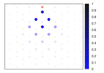
Figure 2: (Color online). The wave function components of an impurity state around a single vacancy which is located on the site denoted by $\times$ symbol in bulk phosphorene.

Now, It is straightforward to calculate the energy correction to this zero-energy mode by the presence of ${\widehat{H}_{1}}$ term in Eq. (2). In doing so, we employ the first order perturbation theory which leads to

$$E_{00}=\langle\Psi_{v}^{A}|{\widehat{H}_{1}}|\Psi_{v}^{A}\rangle=c^{2}\int_{-\pi}^{\pi}\gamma^{-2}(k)2t^{\prime}\cos^{2}{(\frac{k}{2})}dk$$ (9)

with $t^{\prime}=(2t_{4}t_{1})/t_{2}$ in which the integration can be carried out using contour integration Amini2018 . Eqs. (9) and (5) will be used in the next section to calculate the electronic transmission through the edge states of a zPNR in presence of a single vacancy.

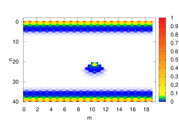
Figure 3: (Color online). Contour plot of the amplitudes of a vacancy state which is located far away from the edges of a zPNR with $(m=20)$ armchair and $(n=40)$ zigzag chains. As a comparison the corresponding amplitudes of edge states is also plotted.

However, before ending this section, let us consider a finite ribbon of phosphorene with zigzag boundary and locate a vacancy far away from the edges. Fig. 3, represents the corresponding LDOS of such a vacancy state which is obtained numerically in agreement with the analytical solution. We can compare our results with the LDOS of the edge states shown along the zigzag edges of the ribbon.

III Fano resonances due to the coupling of a localized state with continuum states

In order to study the phenomenon of Fano resonance, we can consider the impurity state as a quantum dot (QD) coupled to a Q1D quantum system. The Hamiltonian describing the system is

$${\widehat{H}^{\prime}}={\widehat{H}_{Q1D}}+{\widehat{H}_{QD}}+{\widehat{V}},$$ (10)

where the first term is the Hamiltonian of a Q1D lattice with translational invariant which can be written using the plane wave basis $|k\rangle$ as

$${\widehat{H}_{Q1D}}=\int_{-\frac{\pi}{a}}^{\frac{\pi}{a}}E(k)|k\rangle\langle k|dk,$$ (11)

in which $a$ is the lattice constant and $E(k)$ is the energy dispersion relation for electrons moving on the Q1D lattice in the absence of impurity. The second term

$${\widehat{H}_{QD}}=E_{0}|A\rangle\langle A|,$$ (12)

describes a QD with energy $E_{0}$ and, finally, the last term describes the coupling between QD and Q1D as follows

$${\widehat{V}}=\int_{-\frac{\pi}{a}}^{\frac{\pi}{a}}\{u(k)|k\rangle\langle A|+hc.\}dk,$$ (13)

in which $u(k)$ is the coupling strength at momentum $k$. From now on, we set the lattice spacing to one, $a=1$.

Since we are interested in the transmission coefficient $T(E)=|\mathcal{T}|^{2}$ (where $\mathcal{T}$ is the transmission amplitude), we can start with the Lippmann-Schwinger equation in the scattering theory

$$|\psi_{out}\rangle=|\psi_{in}\rangle+{\widehat{G}}_{0}{\widehat{T}}|\psi_{in}\rangle,$$ (14)

where

$${\widehat{T}}(E)={\widehat{V}}{\widehat{G}}_{0}(E){\widehat{V}}+{\widehat{V}}{\widehat{G}}_{0}(E){\widehat{V}}{\widehat{G}}_{0}(E){\widehat{V}}+...,$$ (15)

in which ${\widehat{G}}_{0}(E)$ is the Green’s operator in the absence of coupling between Q1D and QD. Since $\langle A|k\rangle=0$, it is formally possible to write

$${\widehat{G}}_{0}(E)={\widehat{G}}_{0}^{Q1D}(E)+{\widehat{G}}_{0}^{QD}(E),$$ (16)

in which

$${\widehat{G}}_{0}^{Q1D}(E)=\int_{-\pi}^{\pi}\frac{|k\rangle\langle k|}{E-E(k)+i0^{+}}dk,$$ (17)

and

$${\widehat{G}}_{0}^{QD}=\frac{|A\rangle\langle A|}{E-E_{0}+i0^{+}},$$ (18)

are the Green’s functions of clean Q1D and QD respectively. With these expressions in hand, the first term of the series in Eq. (15) can be evaluated as

$${\widehat{V}}{\widehat{G}}_{0}(E){\widehat{V}}=(|A\rangle\langle A|)g+\big{(}\int_{-\pi}^{\pi}(|k^{\prime}\rangle\langle k|)u(k)u(k^{\prime})dkdk^{\prime}\big{)}g^{\prime}$$ (19)

where

$$g(E)=\int_{-\pi}^{\pi}\frac{|u{(k)}|^{2}}{E-E{(k)}+i0^{+}}dk,$$ (20)

and

$$g^{\prime}(E)=\frac{1}{E-E_{0}+i0^{+}}.$$ (21)

Doing the same analysis for the second term in Eq. (15) and collecting these equations, we find,

$${\widehat{T}}(E)=\frac{{\widehat{V}}+{\widehat{V}}^{\prime}}{1-g(E)g^{\prime}(E)},$$ (22)

where we defined

$${\widehat{V}}^{\prime}=g^{\prime}\int_{-\pi}^{\pi}u{(k)}u{(k^{\prime})}|k^{\prime}\rangle\langle k|dk\,dk^{\prime}+g(|A\rangle\langle A|).$$ (23)

According to Eq. (14), the transmission amplitude at energy $E$ can be obtained as,

$$\mathcal{T}(E)=1+\langle k_{0}|{\widehat{G}}_{0}{\widehat{T}}|k_{0}\rangle$$ (24)

for an incident state $|k_{0}\rangle$ such that $E(k_{0})=E$, hence,

$$\mathcal{T}(E)=1+\frac{\frac{|u{(k_{0})}|^{2}}{E-E_{0}}\int_{-\pi}^{\pi}\frac{1}{E-E{(k)}+i0^{+}}dk}{1-\frac{1}{E-E_{0}}\int_{-\pi}^{\pi}\frac{|u{(k)}|^{2}}{E-E{(k)}+i0^{+}}dk}.$$ (25)

By having a quick look at the final expression for $\mathcal{T}(E)$, we can see that the coupling of an extra state (due to the presence of QD) with the continuum states with the same energy can induce an antiresonance in the transmission amplitude. We will use this formalism in the next section to find this kind of resonant scattering due to the presence of vacancies in zPNRs.

III.1 Antiresonance scattering of a 1D chain coupled to a QD

There is, however, at least one task remaining, namely, to show that the above formalism works fine. In order to check our formalism, let us consider the trivial example of scattering of an electron traveling along a 1D chain by a QD (as shown in Fig. 4) which can be described by the Fano–Anderson tight-binding Hamiltonian FlachRMP . The energy dispersion of this model is given by

$$E(k)=2t^{\prime}\,\cos{(k)}$$ (26)

where $t^{\prime}$ is the hopping energy cost of an electron to the nearest neighbor sites. We also consider a QD which is attached to the chain with on-site energy $E_{0}$ and coupling constant $u(k)=u$. Therefore, the resulting transmission is obtained by substituting these parameters into Eq. (25) which yields the following expression

$$\mathcal{T}(E)=1+\frac{\frac{u^{2}}{2it^{\prime}\sin{(k_{0})}}\times\frac{1}{E-E_{0}}}{1-\frac{u^{2}}{2it^{\prime}\sin{(k_{0})}}\times\frac{1}{E-E_{0}}}$$ (27)

where $E_{0}=E(k_{0})$. Hence, we arrive at the exact solution Orellana for the Fano antiresonance in the transmission amplitude of this system.

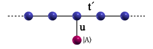
Figure 4: (Color online). Schematic representation of a 1D chain with hopping amplitude $t^{\prime}$ to the nearest neighbors. An impurity state $|A\rangle$ is coupled with amplitude $u$ to the chain.

IV Fano resonances in vacant zPNRs

In this section, we use the above formalism to study the Fano resonance phenomenon which is induced by the presence of a single vacancy defect in ZPNRs. In so doing, our approach is very similar to what was followed in the previous section for a 1D chain coupled to a QD. Let us consider a single vacancy which is located at the $n_{0}$th zigzag chain with respect to the edge of ribbon as shown in Fig. 5.

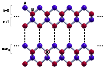
Figure 5: (Color online). Schematic representation of a zPNR lattice structure with a single vacancy located on the $n_{0}$th zigzag chain with respect to the edge.

As we already discussed, this vacancy introduces an additional impurity state whose wave function is $|\Psi_{v}^{A}\rangle$. Now, the significant idea is that we would replace the role of Q1D and QD systems by the edge modes of the zPNR and vacancy state respectively. Accordingly, we need to replace the required quantities $E(k)$, $E_{0}$ and $u(k)$ in Eq. (25) with their counterparts of the vacant zPNR. This will be demonstrated shortly.

Let us start with first quantity $E(k)$ which is the electronic energy dispersion relation of the edge states in zPNR which is obtained in Ref. Amini2018 as

$$E(k)=\langle\Psi^{A}(k)|{\widehat{H}_{1}}|\Psi^{A}(k)\rangle=-2t^{\prime}(1+\cos{(k)}).$$ (28)

Before proceeding to the other quantities, we need to solve a technical problem. It is important to note that according to Eqs. (4) and (5), the states $|\Psi^{A}(k)\rangle$ and $|\Psi_{v}^{A}\rangle$ are not orthogonal, namely $\langle\Psi^{A}(k)|\Psi_{v}^{A}\rangle\neq 0$. Thus, we need to define an orthogonal state $|{\Psi^{\prime}}_{v}^{A}\rangle$ as

$$|{\Psi^{\prime}}_{v}^{A}\rangle=c^{\prime}\left(|\Psi_{v}^{A}\rangle-\int_{-\pi}^{\pi}\langle\Psi_{v}^{A}|\Psi^{A}(k)\rangle|\Psi^{A}(k)\rangle dk\right)$$ (29)

such that the required condition $\langle\Psi^{A}(k)|{\Psi^{\prime}}_{v}^{A}\rangle=0$ is satisfied. Here,

$$(c^{\prime})^{-2}=1-c^{-2}\int_{-\pi}^{\pi}\alpha^{4}(k)\gamma^{-2}(k)dk$$ (30)

is a constant that can be used to normalize the wave function. It is now possible to obtain the energy of this bound state which resembles the quantity $E_{0}$. Due to the presence of the term ${\widehat{H}_{1}}$ the corresponding bound-state energy of $|{\Psi^{\prime}}_{v}^{A}\rangle$ is changed from zero and can be obtained perturbatively as

$$E^{\prime}_{0}=\langle{\Psi^{\prime}}_{v}^{A}|{\widehat{H}_{1}}|{\Psi^{\prime}}_{v}^{A}\rangle=\left(E_{00}-E_{01}-E_{10}^{*}+E_{11}\right),$$ (31)

where $E_{ij}$s are given by

$$E_{01}=c^{2}\int_{-\pi}^{\pi}2t^{\prime}\gamma^{-2}(k)\cos^{2}{(k/2)}\left[\alpha^{2n_{0}-2}(k)+\alpha^{2n_{0}}(k)\right],$$ (32)

and

$$E_{11}=c^{2}\int_{-\pi}^{\pi}4t^{\prime}\gamma^{-2}(k)\cos^{2}{(k/2)}\alpha^{2n_{0}}(k).$$ (33)

$E_{00}$ is given by Eq. (9) and $E_{10}^{*}=E_{01}$. It is now important, however, to note that if the bound state energy $E^{\prime}_{0}$ lies within the energy interval of the edge modes, namely $-2t^{\prime}<E^{\prime}_{0}<0$, then it is expected to observe the Fano antiresonance for the edge modes. For instance,

$$E^{\prime}_{0}=0.00\,\,\,\,for\,\,\,\,n_{0}=0$$ (34a)

$$E^{\prime}_{0}=-0.11\,\,\,\,for\,\,\,\,n_{0}=1$$ (34b)

$$E^{\prime}_{0}=-0.14\,\,\,\,for\,\,\,\,n_{0}=2$$ (34c)

$$E^{\prime}_{0}=-0.15\,\,\,\,for\,\,\,\,n_{0}=3.$$ (34d)

which shows that for $n_{0}=0$ one can not observe the Fano antiresonance because it’s corresponding bonding energy lies outside the bandwidth.

We are now in a position to calculate the only remaining quantity $u(k)$ which is the coupling parameter between the vacancy state and edge states, namely

$$u(k)=\langle k|{\widehat{H}_{1}}|{\Psi^{\prime}}_{v}^{A}\rangle.$$ (35)

This results in

$$u(k)={c^{\prime}}^{2}\gamma^{-2}({k})\frac{t_{2}t_{4}}{t_{1}}\left[\alpha^{2n_{0}}({k})-2\alpha^{2n_{0}+2}({k})+\alpha^{2n_{0}+4}({k})\right].$$ (36)

Collecting these results and inserting into Eq. (25), we can obtain the transmission amplitude through the edge states of a zPNR in presence of a single vacancy which is located on $n_{0}$th zigzag chain. Thus,

$$\mathcal{T}{(E)}=1+\frac{\frac{u^{2}{(k_{0})}}{2it^{\prime}\sin(k_{0})}\times\frac{1}{E-E^{\prime}_{0}}}{1-\frac{1}{E-E^{\prime}_{0}}\times\int_{-\pi}^{\pi}\frac{u^{2}{(k)}}{E-2t^{\prime}\cos^{2}(k/2)+i0^{+}}dk}$$ (37)

where $E(k_{0})=E$ and the integration can be carried out analytically using contour integration Amini2018 ; Amini2018-2 .

V Results and discussion

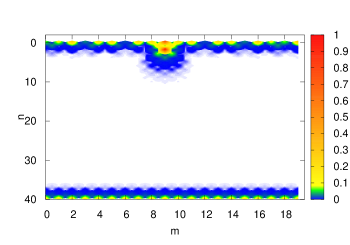
Figure 6: (Color online). Snapshot of the LDOS of edge states and localized state around a single vacancy which is located on the $n_{0}=1$ zigzag chain of a zPNR with 1600 atoms.

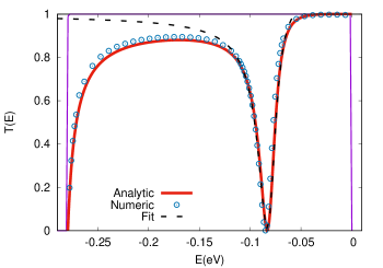
Figure 7: (Color online). Transmission coefficient of an electron traveling along the zigzag edge of a zPNR in presence of a single vacancy which is located on site $(m=0,n_{0}=1,B)$ as a function of incident electron energy. The solid lines corresponds to the analytical results, the black dahsed lines shows the standard Fano line shape fitted to the analytical expression close to the resonance energy, and the discrete circles corresponds to the numerical results obtained using the recursive Green’s function method.

In this section we consider a zPNR in presence of a single vacancy which is located at site $(m=0,n_{0},B)$. As we already discussed, only when $n_{0}\geq 1$ the Fano antiresonance takes place. Therefore, for simplicity, we first assume $n_{0}=1$ which is the first place in which the vacancy can induce antiresonance. In Fig. 6 we show the corresponding LDOS of the edge states and localized vacancy state obtained numerically. In order to obtain the transmission amplitude of such a system, we can insert Eqs. (31) and (36) into Eq. (37) which results in

$$\mathcal{T}{(E)}=1+\frac{\frac{|u{(k_{0})}|^{2}}{2it^{\prime}\sin(k_{0})}\times\frac{1}{E-E^{\prime}_{0}}}{1-\frac{1}{E-E^{\prime}_{0}}\times\frac{\beta{(k_{0})}}{2it^{\prime}\sin(k)}}$$ (38)

in which $E^{\prime}_{0}$ and $u(k)$ should be evaluated for $n_{0}=1$ and $\beta{(k_{0})}$ is rather a complicated expression which we do not present here. Instead, we present a graphical representation of the transmission coefficient $T(E)$ using the transmission amplitude in Eq. (38) as a function of energy $E$ in Fig. 7. It is clearly shown in Fig. 7 that there exists a Fano antiresonance around resonance energy $E_{r}(n_{0}=1)\approx-0.08$ (and close to it’s corresponding bound state energy $E^{\prime}_{0}$) for which the transmission through the edge channel vanishes. This is due to the destructive interference of the traveling wave which can either bypass the vacancy state or populate it and return back to the continuum. Let us now check the deviation of represented expression from the standard line shape of the Fano resonances FlachRMP of the form

$$T(\varepsilon)=\frac{(\varepsilon+q)^{2}}{\varepsilon^{2}+1},$$ (39)

where $\varepsilon=(E-E_{r})/(\Gamma/2)$ and $\Gamma$, $E_{r}$, and $q$ are the line width, peak position, and asymmetry parameter respectively. Fig. 7 shows the fitted curve (dashed lines) with this Fano formula which shows an excellent agreement to a Fano line shape with asymmetry parameter $q=0.18$. This difference with the case of an exactly 1D chain which shows a symmetric transmission profile is reasonable since the zPNR is a Q1D system and the edge states have non-zero amplitudes within the localization radius near the edge. In order to check our analytical expression, we also use the numerical Landauer approach that works on the basis of the recursive Green’s function technique and we have used it in Ref. Amini2018 . Fig. 7 (discrete circles) shows the resulting transmission which is obtained from the numerical calculation and is in perfect agreement with the analytical solution.

Next, we study the influence of varying the vacancy position on the Fano lineshape properties. To this end, we change the vacancy position to different distances from the edge, namely increasing $n_{0}$ to $n_{0}=2,3$. Fig. 8 presents the transmission probability versus the incident electron energy for various vacancy positions. It is clear that displacing the vacancy away from the edge of the zPNR causes several important differences: (i) a shift in the resonance energy toward the center of the edge band; (ii) suppression of the asymmetry parameter $q$, and (iii) decreasing the line width of the peak, $\Gamma$. The reason is that by increasing the distance of vacancy from the edge, the coupling parameter $u(k)$ decreases due to the suppression of wave functions overlap and since the resonance width is directly proportional to the coupling strength, therefore $\Gamma$ decreases. Furthermore, far away from the edge, one can consider the edge states as an exactly 1D chain, therefore, the transmission profile should be symmetric and locate at the band center. Before ending this discussion, we should emphasize that our results are completely consistent with the results of Ref. Peeters2018 .

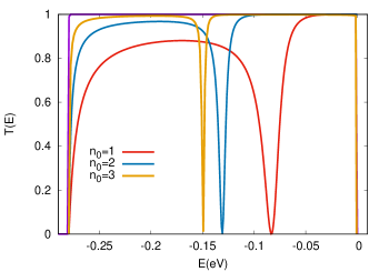
Figure 8: (Color online). The dependence of resonant peak shape and position on the vacancy distance from the edge of zPNR plotted with different colors: red $n_{0}=1$, blue $n_{0}=2$, and orange $n_{0}=3$.

Finally, it is worth pointing out that the presence of hopping parameters $t_{3}$ and $t_{5}$ does not change the overall picture of the transmission coefficient in general. To clarify this point, we present a plot of transmission coefficient versus energy for both cases, namely the case in which $t_{3}=t_{5}=0$ and the case with non-zero $t_{3}$ and $t_{5}$, in Fig. 9. As presented in Fig. 9, the resonant peaks of transmission coefficient in presence of $t_{3}$ and $t_{5}$ (which is shown with dashed lines) takes place with a small energy shift. This is reasonable because the presence of $t_{3}$ and $t_{5}$ increases the energy bandwidth of the edge band.

VI Summary

In this paper, we have demonstrated the existence of a new type of impurity state associated with vacancies in monolayer phosphorene which exhibits a strongly anisotropic localization profile in real space. We found that the localized state induced by vacancies can overlap with the wave functions of the edge states in a confined ribbon of phosphorene which results in the formation of dips in the electronic transmission through the edge modes. The latter takes place when the energy of the vacancy bound state lies inside the quasi flat band composed of the edge modes. We have derived analytically and validated numerically the theory of such antiresonances in zPNRs with a vacancy using the T-matrix Lippmann-Schwinger approach. Modeling the continuum states of the edges of zPNRs as a Q1D system and the vacancy state as a QD, we found that it is exactly a Fano phenomenon due to the coupling of vacancy state to the continuum of the edge modes. We have tried to shed light on various effects of displacing the vacancy on such Fano antiresonances that occur in a zPNR with single vacancies.

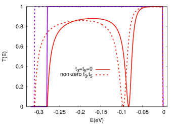
Figure 9: Color online). The effect of none-zero hopping integrals $t_{3}$ and $t_{5}$ on the resonant peak positions induced by a single vacancy which is located at $n_{0}=1$ zigzag chain. The dashed lines obtained in the presence of $t_{3}$ and $t_{5}$ and compared with their counterparts with solid lines when $t_{3}=t_{5}=0$.

- (1) L. Li, Y. Yu, G. J. Ye, Q. Ge, X. Ou, H. Wu, D. Feng, X. H. Chen, and Y. Zhang, Nat. Nanotechnol. 9, 372 (2014).
- (2) L. Li, F. Yang, G. J. Ye, Z. Zhang, Z. Zhu, W. Lou, L. Li, X. Zhou, K. Watanabe, T. Taniguchi, K. Chang, Y. Wang, X. H. Chen, and Y. Zhang, Nat. Nanotechnol. 11, 593 (2016).
- (3) H. Liu, A. T. Neal, Z. Zhu, Z. Luo, X. Xu, D. Tomanek, and P. D. Ye, ACS Nano 8, 4033 (2014).
- (4) F. Xia, H. Wang, and Y. Jia, Nat. Commun. 5, 4458 (2014).
- (5) S. P. Koenig, R. A. Doganov, H. Schmidt, A. H. Castro Neto, and B. Zyilmaz, Appl. Phys. Lett. 104, 103106 (2014).
- (6) X. Ling, H. Wang, S. Huang, F. Xia, and M. S. Dresselhaus, Proc. Natl. Acad. Sci. (USA) 112, 4523 (2015).
- (7) Alexandra Carvalho, Min Wang, Xi Zhu, Aleksandr S. Rodin, Haibin Su and Antonio H. Castro Neto, Nat. Rev. Mater. 1, 16061 (2016).
- (8) J. Qiao, X. Kong, Z. X. Hu, F. Yang, and W. Ji, Nat. Commun. 5, 4475 (2014).
- (9) A. S. Rodin, A. Carvalho, and A. H. Castro Neto, Phys. Rev. Lett. 112, 176801 (2014).
- (10) D. Cakir, H. Sahin, and F. M. Peeters, Phys. Rev. B 90, 205421 (2014).
- (11) T. Low, R. Roldan, H. Wang, F. Xia, P. Avouris, L. M. Moreno, and F. Guinea, Phys. Rev. Lett. 113, 106802 (2014).
- (12) R. Fei and L. Yang, Nano Lett. 14, 2884 (2014).
- (13) S. Yuan, A. N. Rudenko, and M. I. Katsnelson, Phys. Rev. B 91, 115436 (2015).
- (14) M. Ezawa, New Journal of Physics 16, 115004 (2014).
- (15) M. M. Grujic, M. Ezawa, M. Z. Tadic, and F. M. Peeters, Phys. Rev. B 93, 245413 (2016).
- (16) Z. Nourbakhsh and R. Asgari, arXiv:1803.00751(2018).
- (17) M. Amini and M. Soltani, arXiv:1810.03042 (2018).
- (18) W. Hu and J. Yang, J. Phys. Chem. C 119, 20474 (2015).
- (19) V. Wang, Y. Kawazoe, and W. T. Geng, Phys. Rev. B 91, 045433 (2015).
- (20) B. Kiraly, N. Hauptmann, A. N. Rudenko, M. I. Katsnelson, and A. A. Khajetoorians, Nano Lett. 17, 3607 (2017).
- (21) L. L. Li, and F. M. Peeters, Phys. Rev. B 97, 075414 (2018).
- (22) U. Fano Phys. Rev. 124, 1866 (1961).
- (23) A. N. Rudenko, M. I. Katsnelson, Phys. Rev. B 89, 201408 (2014).
- (24) V. M. Pereira, J. M. B. Lopes dos Santos, and A. H. Castro Neto, Phys. Rev. B 77, 115109 (2008).
- (25) V. M. Pereira, F. Guinea, J. M. B. Lopes dos Santos, N. M. R. Peres, and A. H. Castro Neto, Phys. Rev. Lett. 96, 036801 (2006).
- (26) E. V. Castro, M. P. López-Sancho, and M. A. H. Vozmediano, Phys. Rev. Lett. 104, 036802 (2010).
- (27) M. Ezawa, Phys. Rev. B 98, 045125 (2018).
- (28) A. E. Miroshnichenko, S. Flach, and Y. S. Kivshar Rev. Mod. Phys. 82 2257 (2010).
- (29) P. A. Orellana, F. Domínguez-Adame, I. Gómez, and M. L. Ladrón de Guevara, Phys. Rev. B 67, 085321 (2003).
- (30) M. Amini, M. Soltani, E. Ghanbari-Adivi, and M. Sharbafiun arXiv:1810.03486 (2018).