Regularization issues for a cold and dense quark matter model in $\beta$ equilibrium

Abstract

A regularization scheme that explicitly separates vacuum contributions from medium effects is applied to a Nambu–Jona-Lasinio model with diquark interactions and in $\beta$ equilibrium. We perform a comparison of this proposed scheme with the more traditional one, where no separation of vacuum and medium effects is done. Our results point to both qualitative and quantitative important differences between these two methods, in particular regarding the phase structure of the model in the cold and dense nuclear matter case.

I Introduction

Low-energy nonrenormalizable effective models are widely used as a tool to understand many problems in physics when its microscopic, renormalizable counterpart is too complex to be used. This is particularly true in the case of quantum chromodynamics (QCD), where a full use of it becomes not applicable in the context of perturbation theory, like at low energies, given its strong coupling nature. Likewise, the study of the dense nuclear matter through nonperturbative methods based on lattice Monte Carlo QCD simulations (for a recent review, see, e.g., Ref. Ding:2015ona and references therein) is plagued by the so-called “sign problem.” In this context, the use of effective models, for instance the Nambu–Jona-Lasinio (NJL) type of models KLEVAN ; BUBA , is highly valuable to access some otherwise unaccessible region of parameters.

Even in the context of effective models, we still find ultraviolet (UV) divergent momentum integrals that need to be solved. The usual prescription adopted in the literature is to regularize all the divergent momentum integrals through a sharp cutoff $\Lambda$. The momentum cutoff $\Lambda$ in this case is then treated as a parameter of the model, which is fitted by the physical quantities (e.g., by using the pion decay constant, the quark condensate, and pion mass). $\Lambda$ also in a sense sets an energy scale below which in general the effective model should be trusted.

In Refs. Alford1998 ; Rapp1998 the authors showed that the gaps in fermion spectrum are expected to be of the order of 100 MeV and that the possible presence of color superconducting phases could be extended to the region of nonzero temperature on the QCD phase diagram. This is related to the fact that, just like in the case of the usual superconductivity, gaps are related to larger values of critical temperature, which results in a very rich phase structure. In this region the matter consists of three quarks and, depending on the value of the strange ($s$) quark mass, one may observe different types of superconducting phases that can be formed by one, two, or three flavors of quarks. If three quarks do participate in the pairing, the color-flavor locked (CFL) phase is observed Alford:1998mk , while if only the up ($u$) and down ($d$) quarks take place in the pairing, the phase is two color superconductor (2SC) + $s$. It is also possible that only the $s$ quark forms pairs, characterizing a spin-1 condensate that may have influence on some properties of compact stars, as shown, e.g., by Ref. Schmitt:2003xq . If the value of the baryon density is not large enough such that the quark $s$ does not need to be included, we have a pairing of up and down quarks and the corresponding phase is called 2SC. This is the case we are interested in the present work. In Refs. Rajagopal:2000wf ; Alford:2001dt ; Rischke:2003mt there are good reviews on this topic, and in Son1999 ; Shovkovy1999 the authors studied the color superconductivity mechanism at asymptotic densities using first principles calculations. One of the most relevant applications of these studies is to understand the structure of compact stars, where color superconducting phases are expected, since these stars are expected to present densities on their nuclei of the order of 10 $\rho_{0}$, where $\rho_{0}\sim 0.15$ fm^-3 is the saturation density.

In the present work we will make use of the NJL model to study the diquark condensation for a cold and dense quark matter with color and electric charge neutrality. The importance of this model stems from the fact that at sufficiently cold and dense regimes, quark matter behaves as a color superconductor Barrois1977 ; Bailin1984 , where quarks form Cooper pairs with equal and opposite momenta, and studies of QCD under these conditions have many different applications. When studied in the context of the NJL model, which is an intrinsically nonrenormalizable model, we should in principle handle with care the regularization procedure. Even though the regularization scheme is treated as part of the model, it can potentially mix vacuum quantities with medium ones, which can involve explicitly, e.g., chemical potentials, temperature and external fields, or implicilty, through, e.g., a dependence on the various condensates that the system can allow. In principle, one could claim that we are not restricted to follow any prescribed regularization procedure, but we still find that is fair to assume that the model, since it is supposed to be an approximation of a renormalizable one (QCD), hence we believe that preserving those properties observed in the latter case is desirable. One of these properties is that renormalization should in principle only depend on vacuum quantities and not on medium effects. Thus, regularization procedures are required to be done only on vacuum dependent terms, while medium dependent terms should be independent of the regularization chosen to perform UV divergent terms. That this separation of medium effects from regularized vacuum dependent terms only might have not only qualitative but also important quantitative effects was noticed already in Ref. Farias2006 in the context of color superconductivity in a NJL model. A similar situation was also found in the case of studies of magnetized quark matter, where unphysical spurious effects are eliminated by properly separating the magnetic field contributions from the divergent integrals Menezes:2008qt ; Allen2015 ; Duarte:2015ppa ; Coppola2017 . This same procedure has been advocated recently in Ref. Farias:2016let in the context of the NJL model with a chiral imbalance. The process of disentangling the vacuum dependent terms from medium ones and properly regularizing only the UV divergent momentum integrals for the former was named the “medium separation scheme” (MSS) in opposition to the usual procedure where the cutoff is applied even to the medium dependent terms, the traditional regularization scheme (TRS).

One of the most important motivations for our study comes from the fact that there is a great deal of evidence pointing to the increasing of the diquark condensate with the chemical potential. While realistic $N_{c}=3$ QCD lattice simulations cannot be implemented due to the well-discussed sign problem Karsch2002 this is not the case for $N_{c}=2$. Using two colors, the lattice simulations are available, and the results clearly predicts an increase of the diquark condensate with the chemical potential Kogut2001 ; Braguta2016 . This is also indicated by studies using chiral perturbation theory (ChPT) Kogut:2000ek . As we are going to see, in the traditional treatment of divergences in the TRS case, the diquark condensate eventually vanishes, which seems to be at odds with what we would expect in general. By applying the MSS procedure instead, we predict an always increasing diquark condensate. As a side result, we also show an explicit change of behavior in the phases for the diquark condensate as the chemical potential is increased, which is not able to be obtained in the context of the TRS regularization procedure.

This work is organized as follows. In Sec. II, we introduce the NJL model with diquark interactions and give the explicit expression for the thermodynamical potential. In Sec. III we give the MSS regularization procedure and define the appropriate equations for having $\beta$ equilibrium and charge neutrality. In Sec. IV, we show our numerical results comparing TRS and MSS schemes. In Sec. V, we present our conclusions. Three appendixes are also included where we show the more technical details in the MSS calculation and how to write the expressions for the individual densities when $\beta$ equilibrium is included.

II The model and its thermodynamic potential

In this work we study the NJL model with interactions involving the scalar, pseudoscalar and diquark channels for the quark field. The explicit form of the Lagrangian density is then given by

$${\cal L} = \bar{\psi}\left(i\gamma^{\mu}\partial_{\mu}-m\right)\psi+G_{s}\left[\left(\bar{\psi}\psi\right)^{2}+\left(\bar{\psi}i\gamma_{5}\vec{\tau}\psi\right)^{2}\right]$$ (1)

$$+G_{d}\left[\left(i\bar{\psi}^{C}\varepsilon\epsilon^{b}\gamma_{5}\psi\right)\left(i\bar{\psi}\varepsilon\epsilon^{b}\gamma_{5}\psi^{C}\right)\right],$$

where $m$ is the current quark mass, $\psi^{C}=C\bar{\psi}^{T}$ is the charge-conjugate spinor, and $C=i\gamma^{2}\gamma^{0}$ is the charge conjugation matrix. The quark field $\psi\equiv\psi_{i\alpha}$ is a four-component Dirac spinor that carries both flavor $\left(i=1,2\right)$ and color $\left(\alpha=1,2,3\right)$ indices. The Pauli matrices are denoted by $\vec{\tau}=\left(\tau^{1},\tau^{2},\tau^{3}\right)$, while $\left(\varepsilon\right)^{ik}\equiv\varepsilon^{ik}$ and $\left(\epsilon^{b}\right)^{\alpha\beta}\equiv\epsilon^{\alpha\beta b}$ are the antisymmetric tensors in the flavor and color spaces, respectively.

In $\beta$ equilibrium, the diagonal matrix of quark chemical potentials is given in terms of quark, electrical charge, and color charge chemical potentials,

$$\mu_{ij,\alpha,\beta}=\left(\mu\delta_{ij}-\mu_{e}Q_{ij}\right)\delta_{\alpha\beta}+\frac{2}{\sqrt{3}}\mu_{8}\delta_{ij}\left(T_{8}\right)_{\alpha\beta},$$ (2)

where $Q$ and $T_{8}$ are generators of the electromagnetism U(1)${}_{\text{em}}$ and the U(1)₈ subgroup of the color gauge groups, respectively. The explicit expressions for the quark chemical potentials read

$$\mu_{ur} = \mu_{ug}=\mu-\frac{2}{3}\mu_{e}+\frac{1}{3}\mu_{8},$$ (3)

$$\mu_{dr} = \mu_{dg}=\mu+\frac{1}{3}\mu_{e}+\frac{1}{3}\mu_{8},$$ (4)

$$\mu_{ub} = \mu-\frac{2}{3}\mu_{e}-\frac{2}{3}\mu_{8},$$ (5)

$$\mu_{db} = \mu+\frac{1}{3}\mu_{e}-\frac{2}{3}\mu_{8}.$$ (6)

In the mean field approximation, the finite temperature ($T$) effective potential for quark matter in $\beta$ equilibrium with electrons is well known Huang:2003xd ; Shovkovy:2003uu and it is explicitly given by

$$\Omega = \Omega_{0}-\left(\frac{\mu_{e}^{4}}{12\pi^{2}}+\frac{T^{2}\mu_{e}^{2}}{6}+\frac{7\pi^{2}}{180}T^{4}\right)+\frac{\left(M-m\right)^{2}}{4G_{s}}$$ (7)

$$+ \frac{\Delta^{2}}{4G_{d}}-2T\sum_{a}n_{a}\int\frac{d^{3}p}{\left(2\pi\right)^{3}}\ln\left(1+e^{-E_{a}/T}\right)$$

$$- \sum_{a}n_{a}\int\frac{d^{3}p}{\left(2\pi\right)^{3}}E_{a},$$

where $\mu_{e}$ is the electron chemical potential and $\Omega_{0}$ is the constant vacuum energy term added so as to make the pressure of the vacuum zero. In Eq. (7), for simplicity, we have assumed a vanishing value for the electron mass, which is sufficient for the purposes of the current study. The sum in the second line of Eq. (7) runs over all quasiparticles, whose explicit dispersion relations read

$$E_{ub}^{\pm} = E\pm\mu_{ub},$$ (8)

$$E_{db}^{\pm} = E\pm\mu_{db},$$ (9)

$$E_{\Delta^{\pm}}^{\pm} = E_{\Delta}^{\pm}+\delta\mu,$$ (10)

where we have introduced the following notation for convenience:

$$E \equiv \sqrt{p^{2}+M^{2}},$$ (11)

$$E_{\Delta}^{\pm} \equiv \sqrt{\left(E\pm\bar{\mu}\right)^{2}+\Delta^{2}},$$ (12)

$$\bar{\mu} \equiv \frac{\mu_{ur}+\mu_{dg}}{2}=\frac{\mu_{ug}+\mu_{dr}}{2}$$ (13)

$$= \mu-\frac{\mu_{e}}{6}+\frac{\mu_{8}}{3},$$

$$\delta\mu \equiv \frac{\mu_{dg}-\mu_{ur}}{2}=\frac{\mu_{dr}+\mu_{ug}}{2}$$ (14)

$$= \frac{\mu_{e}}{2};$$

in the above equations, $\Delta$ is the diquark condensate and $M$ is the constituent quark mass. The multiplicity $n_{a}$ in Eq. (7) is related to the degeneracy factors of each quasiparticle dispersions, such as $n_{ub}=n_{db}=1$ and $n_{\Delta}=2$ (corresponding to the dispersions $E_{\Delta^{\pm}}^{\pm}$, related to the $r$ and $g$ colors, due to the definitions of $\bar{\mu}$ and $\delta\mu$).

For the demonstration purposes in this work, we can assume, without loss of generality, the chirally symmetric phase of quark matter and, thus, we will work in the chiral limit. In this limit, the quasiparticle dispersions (11) and (12) then become

$$E = p,$$ (15)

$$E_{\Delta}^{\pm} = \sqrt{\left(p\pm\bar{\mu}\right)^{2}+\Delta^{2}}.$$ (16)

The vacuum term $\Omega_{0}$ in Eq. (7) is obtained by considering $\Delta=\mu=\mu_{e}=\mu_{8}=0$ and taking the effective quark mass is its vacuum value, $M_{0}$. Thus, we obtain that

$$\Omega_{0} = -\frac{M_{0}^{2}}{4G_{s}}+12\int\frac{d^{3}p}{\left(2\pi\right)^{3}}\sqrt{p^{2}+M_{0}^{2}}.$$ (17)

Finally, by considering the $T\to 0$ limit in Eq. (7), we obtain that Huang:2003xd

$$\Omega_{T=0}\left(\Delta,\bar{\mu},\delta\mu\right) = \Omega_{0}-\frac{\mu_{e}^{4}}{12\pi^{2}}+\frac{\Delta^{2}}{4G_{d}}-\frac{\mu_{ub}^{4}}{12\pi^{2}}-\frac{\mu_{db}^{4}}{12\pi^{2}}$$ (18)

$$- 2\theta\left(\delta\mu-\Delta\right)\int_{\mu^{-}}^{\mu^{+}}\frac{dp}{\pi^{2}}p^{2}\left(\delta\mu-E_{\Delta}^{-}\right)$$

$$- 4\int\frac{d^{3}p}{\left(2\pi\right)^{3}}\left(p+E_{\Delta}^{+}+E_{\Delta}^{-}\right),$$

where $\mu^{\pm}=\bar{\mu}\pm\sqrt{\delta\mu^{2}-\Delta^{2}}$ and $\Omega_{0}$ is given by Eq. (17).

III Regularization issues and medium effects

The momentum integral in the last term in Eq. (7) and, equivalently, the last one in Eq. (18) when taking the chiral limit are UV divergent. These terms mix vacuum quantities with medium ones. In the case of the last term in Eq. (7), or in the case of Eq. (18), we have contributions that depends explicitly or implicilty in chemical potentials $\mu$, $\mu_{e}$, and $\mu_{8}$, and in the diquark condensate $\Delta$. Integrands with these dependences might not be regularized naively, just introducing a cutoff parameter. As argued in the Introduction, these terms should be handled with care and two regularization procedures can be applied, the TRS and the MSS one. Let us start by discussing the implementation of the MSS procedure as a way to properly disentangle these dependencies of vacuum dependent terms from the medium effects for the present problem. We initially discuss the more general case, the physical case, with a nonvanishing current quark mass $m$. The generalization for the chiral limit for the MSS regularized integrals is immediate.

The gap equation for $\Delta$ is obtained from Eq. (7) by deriving it with respect to $\Delta$. Let us concentrate on the UV divergent term that results from the last term in Eq. (7). Its contribution for the gap equation for $\Delta$ is of the form

$$I_{\Delta} = \int\frac{d^{3}p}{\left(2\pi\right)^{3}}\left(\frac{1}{E_{\Delta}^{+}}+\frac{1}{E_{\Delta}^{-}}\right)$$ (19)

$$= \sum_{s=\pm 1}\int\frac{d^{3}p}{\left(2\pi\right)^{3}}\frac{1}{E_{\Delta}^{s}}\,,$$

with $E_{\Delta}^{s}=\sqrt{\left(E+s\bar{\mu}\right)^{2}+\Delta^{2}}$. This term can be rewritten as

$$\int\frac{d^{3}p}{\left(2\pi\right)^{3}}\frac{1}{E_{\Delta}^{s}}=\frac{1}{\pi}\int_{-\infty}^{+\infty}dp_{4}\int\frac{d^{3}p}{\left(2\pi\right)^{3}}\frac{1}{p_{4}^{2}+(E_{\Delta}^{s})^{2}}\,,$$ (20)

such that

$$\frac{1}{2}\sum_{s=\pm 1}\int\frac{d^{3}p}{\left(2\pi\right)^{3}}\frac{1}{E_{\Delta}^{s}}$$ (21)

$$=\sum_{s=\pm 1}\int_{-\infty}^{+\infty}\frac{dp_{4}}{2\pi}\int\frac{d^{3}p}{\left(2\pi\right)^{3}}\frac{1}{p_{4}^{2}+(E_{\Delta}^{s})^{2}}.$$

Making use of the identity Battistel1999 ,

$$\frac{1}{p_{4}^{2}+\left(E+s\bar{\mu}\right)^{2}+\Delta^{2}}$$ (22)

$$=\frac{1}{p_{4}^{2}+p^{2}+M_{0}^{2}}$$

$$-\frac{\mu^{2}+2sE\mu+\Delta^{2}+M^{2}-M_{0}^{2}}{\left(p_{4}^{2}+E^{2}+M_{0}^{2}\right)\left[p_{4}^{2}+\left(E+s\bar{\mu}\right)^{2}+\Delta^{2}\right]},$$

we obtain, after making two iterations of this same identity, the result

$$\frac{1}{p_{4}^{2}+\left(E+s\bar{\mu}\right)^{2}+\Delta^{2}}$$ (23)

$$=\frac{1}{p_{4}^{2}+p^{2}+M_{0}^{2}}+\frac{A-2sE\bar{\mu}}{\left(p_{4}^{2}+p^{2}+M_{0}^{2}\right)^{2}}$$

$$+\frac{\left(A-2sE\bar{\mu}\right)^{2}}{\left(p_{4}^{2}+p^{2}+M_{0}^{2}\right)^{3}}$$

$$+\frac{\left(A-2sE\bar{\mu}\right)^{3}}{\left(p_{4}^{2}+p^{2}+M_{0}^{2}\right)^{3}\left[p_{4}^{2}+\left(E+s\bar{\mu}\right)^{2}+\Delta^{2}\right]},$$

with $A=M_{0}^{2}-M^{2}-\bar{\mu}^{2}-\Delta^{2}$. Thus, after performing some simple algebraic manipulations, the sum in $s$ and also the $p_{4}$ integrations, as indicated in Eq. (21), can be made and we obtain the result

$$\sum_{s=\pm 1}\int_{-\infty}^{+\infty}\frac{dp_{4}}{2\pi}\int\frac{d^{3}p}{\left(2\pi\right)^{3}}\frac{1}{p_{4}^{2}+(E_{\Delta}^{\pm})^{2}}$$ (24)

$$=I_{\text{quad}}-\frac{\left(\Delta^{2}-M_{0}^{2}-2\bar{\mu}^{2}+M^{2}\right)}{2}I_{\text{log}}-I_{\text{fin,2}}$$

$$+\left[\frac{3\left(A^{2}+4M^{2}\bar{\mu}^{2}\right)}{8}-\frac{3\bar{\mu}^{2}M_{0}^{2}}{2}\right]I_{\text{fin,1}},$$

where we have defined the quantities

$$I_{\text{quad}} = \int\frac{d^{3}p}{\left(2\pi\right)^{3}}\frac{1}{\sqrt{p^{2}+M_{0}^{2}}},$$ (25)

$$I_{\text{log}} = \int\frac{d^{3}p}{\left(2\pi\right)^{3}}\frac{1}{\left(p^{2}+M_{0}^{2}\right)^{\frac{3}{2}}},$$ (26)

$$I_{\text{fin,1}} = \int\frac{d^{3}p}{\left(2\pi\right)^{3}}\frac{1}{\left(p^{2}+M_{0}^{2}\right)^{\frac{5}{2}}},$$ (27)

$$I_{\text{fin,2}} = \frac{15}{32}\sum_{s=\pm 1}\int\frac{d^{3}p}{\left(2\pi\right)^{3}}\int_{0}^{1}dx(1-x)^{2}$$ (28)

$$\times \frac{(A-2sE\bar{\mu})^{3}}{\left[(2sE\bar{\mu}-A)x+p^{2}+M_{0}^{2}\right]^{\frac{7}{2}}}.$$

Comparing Eq. (19) and the left-hand side of Eq. (21) we can see that

$$\frac{1}{2}I_{\Delta}=\sum_{s=\pm 1}\int_{-\infty}^{+\infty}\frac{dp_{4}}{2\pi}\int\frac{d^{3}p}{\left(2\pi\right)^{3}}\frac{1}{p_{4}^{2}+(E_{\Delta}^{\pm})^{2}},$$ (29)

and, therefore,

$$I_{\Delta} = 2I_{\text{quad}}-\left(\Delta^{2}-M_{0}^{2}-2\bar{\mu}^{2}+M^{2}\right)I{}_{\text{log}}+2I_{\text{fin,2}}$$ (30)

$$+ \left[\frac{3(A^{2}+4M^{2}\bar{\mu}^{2})}{4}-3M_{0}^{2}\bar{\mu}^{2}\right]I_{\text{fin,1}}.$$

It is important to note that Eq. (30) was not evaluated in the chirally symmetric phase; i.e., it can also be used for studying the system before the chiral phase transition or in the physical limit. In the physical case we have an additional gap equation for the mass $m$ that can be evaluated in the MSS procedure by using the same manipulations used to evaluate $I_{\Delta}$. The $m\to 0$ limit to study the chiral phase is trivial and it is taken in the calculations to be presented below.

IV Contrasting the TRS and MSS regularization procedures

To obtain the numerical results for $N_{c}=3$ in $\beta$ equilibrium we first evaluate the gap equation for $\Delta$, the charge neutrality conditions for $\mu_{8}$ and $\mu_{e}$, and the densities from Eq. (18). For comparison purposes, we will present the results for both schemes, TRS and MSS.

IV.1 The $\Delta$ gap equation

The gap equation is given by

$$\frac{\partial\Omega_{T=0}}{\partial\Delta}\Bigr{|}_{\Delta=\Delta_{c}}=0,$$ (31)

where $\Delta_{c}$ is the solution of

$$1=2G_{d}\left[4I_{\Delta}^{i}-2\theta\left(\delta\mu-\Delta_{c}\right)\int_{\mu^{-}}^{\mu^{+}}\frac{dp}{\pi^{2}}\frac{p^{2}}{E_{\Delta_{c}}^{-}}\right],$$ (32)

where $I_{\Delta}$ is given, in the TRS and MSS cases respectively by

$$I_{\Delta}^{TRS} = \int_{\Lambda}\frac{d^{3}p}{\left(2\pi\right)^{3}}\left(\frac{1}{E_{\Delta}^{+}}+\frac{1}{E_{\Delta}^{-}}\right),$$ (33)

$$I_{\Delta}^{MSS} = 2I_{\text{quad}}-\left(\Delta^{2}-M_{0}^{2}-2\mu^{2}\right)I{}_{\text{log}}+2I_{\text{fin,2}}$$ (34)

$$+ \left[\frac{3\left(M_{0}^{2}-\bar{\mu}^{2}-\Delta^{2}\right)^{2}}{4}-3M_{0}^{2}\bar{\mu}^{2}\right]I_{\text{fin,1}},$$

where the indicated integrals were defined in the previous section, Eqs. (25) - (28), in the limit $m\to 0$, and $E_{\Delta}^{\pm}$ are defined in Eq. (16).

IV.2 The color neutrality condition

It has been widely discussed in the literature that the superconducting quark matter that may occur in compact stars is required to be both electromagnetic and color neutral, such as to be in the stable bulk phase Amore2002 ; Steiner2002 ; Huang2003 . The color neutrality represents the equality between the numbers of quarks with colors red, green, and blue, since the quark matter must be composed by color singlets. In Ref. Amore2002 the authors have shown that once a macroscopic chunk of color superconductor is color neutral, implementation of the projection which imposes color singletness has a negligible effect on the free energy of the state, similar to the usual fact from ordinary superconductivity. In this case, the projection which turns a BCS state, wherein the particle number is formally indefinite, into a state with definite but very large particle number has no significant effect. Color singletness follows without paying any further free energy price Alford2002 . It is important to mention that by imposing these constraints, the free energy of the 2SC phase becomes extremely large and cannot be found in nature. This problem disappears if we also consider the $s$ quark, in which case the phase of the system is CFL, which satisfies the neutrality constraints, costing a smaller quantity of free energy.

In this work we are focused on the correct separation of vacuum divergences, from finite integrals, as well as the influence of the regularization scheme on the values of the diquark condensate and, consequently, in the phase diagrams of the system when $\beta$ equilibrium and charge neutrality are taken into account. For this reason, we will be working simply with the $SU(2)$ version of the NJL model, in which case, due to the definitions (3) to (6), only quarks with red and green colors do participate in the pairing.

The color neutrality condition is obtained by imposing that the number density $n_{8}$ be vanishing. Thus, it is required that

$$n_{8} = -\frac{\partial\Omega_{T=0}}{\partial\mu_{8}}=0,$$ (35)

which leads to the condition

$$0 = -\frac{\mu_{ub}^{3}}{3\pi^{2}}-\frac{\mu_{db}^{3}}{3\pi^{2}}+2I_{8}^{i}+2\bar{\mu}I_{\Delta}^{i}$$ (36)

$$+ \theta\left(\delta\mu-\Delta\right)\int_{\mu^{-}}^{\mu^{+}}\frac{dp}{\pi^{2}}p^{2}\,\frac{p-\bar{\mu}}{E_{\Delta}^{-}},$$

with $I_{\Delta}^{i}$ defined in Eq. (33) or (34), for the TRS or MSS cases, respectively, and $I_{8}^{i}$ is given by

$$I_{8}^{TRS} = \int_{\Lambda}\frac{d^{3}p}{\left(2\pi\right)^{3}}\left(\frac{p}{E_{\Delta}^{+}}-\frac{p}{E_{\Delta}^{-}}\right),$$ (37)

$$I_{8}^{MSS} = -2\bar{\mu}I_{\text{quad}}+\bar{\mu}\left(3\Delta^{2}-M_{0}^{2}-2\bar{\mu}^{2}\right)I_{\text{log}}+I_{\text{fin,5}}$$ (38)

$$+ M_{0}^{2}\bar{\mu}\left(3M_{0}^{2}+2\bar{\mu}^{2}-3\Delta^{2}\right)I_{\text{fin,1}}$$

$$+ \frac{5\bar{\mu}}{4}\left[4M_{0}^{2}\bar{\mu}^{2}-3\left(M_{0}^{2}-\bar{\mu}^{2}-\Delta^{2}\right)^{2}\right]I_{\text{fin,4}}.$$

In Appendix A we give some of the details on the explicit calculation of $I_{8}^{MSS}$ and present there also the definitions of $I_{\text{fin,4}}$ and $I_{\text{fin,5}}$.

IV.3 The electric neutrality condition

When considering the electric neutrality condition, we must note that the integrands have the same structure as the ones in $n_{8}$. Then, by imposing that

$$n_{e} = -\frac{\partial\Omega_{T=0}}{\partial\mu_{e}}=0,$$ (39)

we obtain that

$$0 = \frac{\mu_{e}^{3}}{3\pi^{2}}-\frac{2\mu_{ub}^{3}}{9\pi^{2}}+\frac{\mu_{db}^{3}}{9\pi^{2}}-\frac{2}{3}\bar{\mu}I_{\Delta}^{i}-\frac{2}{3}I_{8}^{i}$$ (40)

$$+ 2\theta\left(\delta\mu-\Delta\right)\int_{\mu^{-}}^{\mu^{+}}\frac{dp\,p^{2}}{\pi^{2}}\left(\frac{1}{2}-\frac{p-\bar{\mu}}{6E_{\Delta}^{-}}\right),$$

where $I_{\Delta}^{i}$ and $I_{8}^{i}$ are given by Eqs. (33) and (37), for the TRS case, or by Eqs. (34) and (38), for the MSS case.

IV.4 The results

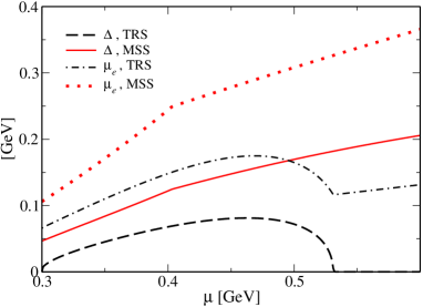
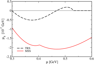
Figure 1: The diquark condensate $\Delta$ and the electron chemical potential $\mu_{e}$ (a) and the color chemical potential $\mu_{8}$ (b), as functions of $\mu$, for both the TRS and MSS regularization schemes.

To obtain our numerical results, we consider the values for the parameters in the NJL model as chosen in the usual way, by the fitting with the experimental vacuum values of the pion decay constant $f_{\pi}=93$ MeV and chiral condensate $\left\langle\bar{\psi}_{f}\psi_{f}\right\rangle^{1/3}=-250$ MeV. The third parameter, the use of the pion mass $m_{\pi}$, is not required if we stay in the chiral limit. The model parameters in this case are found simply to be given by the values $G_{s}=5.0163$ GeV^-2 for the scalar quark four-fermion interaction term, while the ultraviolet cutoff scale is found to be $\Lambda=653.3$ MeV. The diquark coupling constant $G_{d}$ is set to be proportional to $G_{s}$, with the value chosen as $G_{d}=0.75G_{s}$ BUBA ; Huang2003 .

In Fig. 1 we show the results for $\Delta,\,\mu_{e}$, and $\mu_{8}$, obtained by solving numerically Eqs. (32), (36), and (40) in both the TRS and MSS regularization procedures. Note that the result for $\Delta$ initially increases with the chemical potential in both TRS and MSS regularization procedures, but as $\mu$ gets sufficiently large, $\mu\sim 0.53$ GeV, the result for TRS drops down and it is vanishing from then on. The result for MSS still grows with $\mu$ as expected in general grounds. Note also the change in behavior for both the chemical potentials $\mu_{e}$ and $\mu_{8}$ in both regularization schemes. Even for small values for the chemical potential, there are significant quantitative differences in the results obtained in the TRS and MSS procedures.

To emphasize the differences between the TRS and MSS, we also show some of the relevant thermodynamic quantities to compare them between the two methods. First of all, to obtain the baryon density $\rho_{B}$ we need to determine the total density $\rho_{T}=\rho_{u}+\rho_{d}$ in the $SU(2)$ case. However, our expression for the thermodynamic potential, Eq. (18), is written in terms of $\bar{\mu}$ and $\delta\mu$. Here, we restrict ourselves to show the final expressions for each quantity, whose details for their derivation are given in the Appendix C. The individual densities $\rho_{u}$ and $\rho_{d}$ are given by

$$\rho_{u} = \frac{\mu_{ub}^{3}}{3\pi^{2}}+2I_{8}^{i}+2\bar{\mu}I_{\Delta}^{i}+\theta\left(\delta\mu-\Delta\right)\int_{\mu^{-}}^{\mu^{+}}\frac{dp}{\pi^{2}}p^{2}\left(\frac{p-\bar{\mu}}{E_{\Delta}^{-}}\right)$$ (41)

$$- \frac{2\sqrt{\delta\mu^{2}-\Delta^{2}}}{3\pi^{2}}\left(\delta\mu^{2}-\Delta^{2}+3\bar{\mu}^{2}\right)\theta\left(\delta\mu-\Delta\right),$$

and

$$\rho_{d} = \frac{\mu_{db}^{3}}{3\pi^{2}}+2I_{8}^{i}+2\bar{\mu}I_{\Delta}^{i}+\theta\left(\delta\mu-\Delta\right)\int_{\mu^{-}}^{\mu^{+}}\frac{dp}{\pi^{2}}p^{2}\left(\frac{p-\bar{\mu}}{E_{\Delta}^{-}}\right)$$ (42)

$$+ \frac{2\sqrt{\delta\mu^{2}-\Delta^{2}}}{3\pi^{2}}\left(\delta\mu^{2}-\Delta^{2}+3\bar{\mu}^{2}\right)\theta\left(\delta\mu-\Delta\right),$$

where $I_{8}^{i}$ and $I_{\Delta}^{i}$ were already defined previously for each of the two schemes. The normalized pressure $p_{N}$, the baryon density $\rho_{B}$ and the energy density $\varepsilon$ are then given, respectively, by

$$p_{N} = -\Omega_{T=0}\left(\Delta,\bar{\mu},\delta\mu\right),$$ (43)

$$\rho_{B} = \frac{\rho_{T}}{3},$$ (44)

$$\varepsilon = -p_{N}+\mu_{B}\rho_{B}\left(=-p_{N}+3\mu\rho_{B}\right).$$ (45)

The numerical results for these quantities, as well as the individual densities and the equation of state, $p_{N}\times\varepsilon_{N}$, are shown in Figs. 2 and 3. Though the differences in the EoS are not very significant in both the regularization schemes, the energy density and pressure tend to increase faster in the MSS case than in the TRS one.

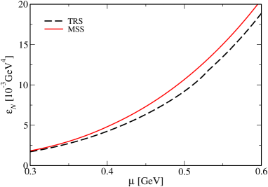
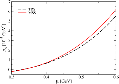
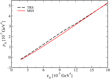
Figure 2: The energy density (a), the normalized pressure (b), and the equation of state (c) as functions of $\mu$, for both the TRS and MSS regularization schemes.

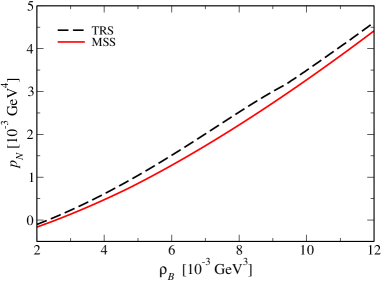
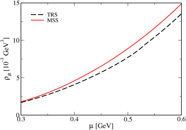
Figure 3: The normalized pressure as a function of the baryon density (a) and the baryon and individual densities $\rho_{u}$ and $\rho_{d}$ (b) as functions of the chemical potential $\mu$, for both the TRS and MSS regularization schemes.

Figure 4: The criterion $\delta\mu-\Delta$ used to define a g2SC or 2SC phase of the system in the cases of the TRS and MSS regularization procedures.

It is argued in the literature Huang:2003xd ; Shovkovy:2003uu that a neutral 2SC phase exists at low values of $\mu$, called th “gapless-2SC” (g2SC) phase, instead of the usual 2SC one (for a detailed discussion regarding the gapless phase, structure, and consequences, see in addition revCSC and references therein). The criterion used to define whether the system is in the gapless or in the 2SC phase is quite simple. In $\beta$ equilibrium the new contribution to the effective potential is exactly the term that contains a step function on Eq. (18). If $\delta\mu>\Delta$, this term remains and the phase is said to be in the g2SC. Otherwise, for $\delta\mu<\Delta$, that term disappears and the phase is said to be in the usual 2SC one. In Fig. 4 we probe the emergence of these two possible phases.

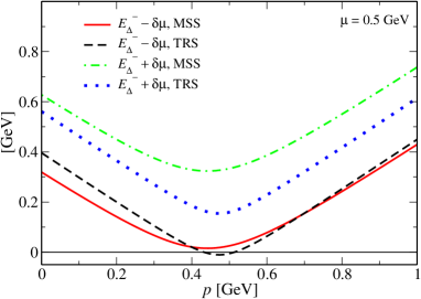
Figure 5: Quasiparticle dispersion relations $E_{\Delta}^{-}\pm\delta\mu$, for (a) $\mu=0.35$ GeV and (b) $\mu=0.5$ GeV.

It is also useful to discuss the difference between the g2SC and 2SC phases from the dispersion relations for quasiparticles in the context of the two regularization schemes studied here. From Eqs. (41) and (42) one can see that in g2SC the pairing quarks have different number densities, which does not occur in 2SC. The spectrum in the 2SC case includes the free blue quark that does not take place in the pairing and also the quasiparticle excitations formed by the linear superposition of $u_{rg}$ and $d_{rg}$ quarks, whose gap is $\Delta$. When $\delta\mu\neq\Delta$, there is a small discrepancy between the Fermi surfaces of the $u$ and $d$ pairing quarks, shifting one of the dispersions to $\Delta+\delta\mu$ and the other to $\Delta-\delta\mu$. When the mismatch $\delta\mu>\Delta$, the lower dispersion relation becomes negative for some values of $p$ and this is the spectrum usually called gapless. This is illustrated in Fig. 5. For $\mu=0.35$ GeV, both regularization schemes predict a gapless phase for the system, even though in the MSS case the value of $E_{\Delta}^{-}-\delta\mu$ is smaller (in magnitude) than in the TRS case. On the other hand, for $\mu=0.5$ GeV, the dispersion for the MSS never becomes negative; i.e., the system is in the 2SC phase, while in the TRS the gapless phase is observed again.

One can see that using the MSS regularization procedure the behavior of the phase structure can become quite different. While in the TRS case the system is always in the g2SC phase in the range of $\mu$ considered in this work, the situation becomes quite the opposite in the case of the MSS regularization procedure. We can see from the results shown in Figs. 4 and 5 that now the system can display a transition between the g2SC and the 2SC phases. This is quite a remarkable difference and it is the main result of this work. We can trace this change of behavior in the MSS case by recalling the result shown in Fig. 1 for the diquark condensate $\Delta$. In the TRS case, the diquark condensate never increases to be above $\delta\mu$ and, even worse, it vanishes after $\mu\gtrsim 0.53$ GeV. However, in the MSS, $\Delta$ is larger than in the TRS case and always increases with the chemical potential. Thus, it is no wonder that at some point it will become larger than $\delta\mu$ and the system can transit from a g2SC to a 2SC phase. It is nice to see that this can happen already for not relatively too large values of the chemical potential. This is also reflected on the behavior of thermodynamic quantities. From Figs. 2 and 3, one notices that the difference between two schemes increases with the increase of the chemical potential. This is related to the change to the 2SC phase in the MSS case, while in the TRS case the system is still in the g2SC phase.

Finally, it is also useful to comment on the effect of the value of the diquark interaction $G_{d}$ on the results. In all of the above results, we have used $G_{d}=3G_{s}/4$, a value naturally motivated when deriving the Lagrangian density Eq. (1) from the QCD one-gluon exchange approximation and it results from the Fierz transform of the primary color current-current coupling, projected into the relevant quark-antiquark and diquark channels BUBA . However, it is quite common in the literature to simply consider $G_{d}$ as an additional free parameter of the model. In Fig. 6(a) we show the results for the diquark condensate and in Fig. 6(b) the results equivalent to Fig. 4, as a function of some representative values of the ratio $G_{d}/G_{s}\equiv\eta$, to illustrate the differences that appear when using the TRS or the MSS procedures.

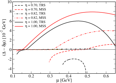
Figure 6: Diquark condensate (a) and the change from the g2SC to the 2SC phases (b), as a function of the chemical potential and for different values of the ratio $G_{d}/G_{s}\equiv\eta$.

From the results shown in Fig. 6, we see that the differences between the TRS and MSS procedures are more pronounced for values of $\eta<1$. As we increase $\eta$, the differences decrease, but they are still evident and quantitatively large as the chemical potential increases. In particular, we still see a decrease of the diquark condensate $\Delta$ in the TRS case even when $\eta=1$. For a ratio of $\eta\gtrsim 0.82$, we see from Fig. 6(b) that the TRS can also display a transition from the g2SC to the 2SC phase, yet, the difference with the MSS case is always appreciable. It is also important to mention that if we consider lower values of $\eta$, the system is in the gapless phase for larger values of $\mu$ in MSS, and the value of $\Delta$ becomes smaller for both schemes. For $\eta\sim 0.68$, we did not find solutions for $\Delta\neq 0$ using TRS, and the color superconducting phase is not predicted in this scheme.

V Conclusions

In this work we have studied an alternative regularization approach where medium effects are explicitly separated from vacuum dependent terms and UV divergent momentum integrals become only dependent on the vacuum quantities. We have applied this to the NJL model with diquark interactions and in $\beta$ equilibrium. We perform an explicit comparison of this proposed scheme, called the MSS regularization procedure, with the more traditional one, the TRS regularization procedure, where no separation of vacuum and medium effects is done. Our results point to both qualitatively and quantitatively important differences between these two methods, in particular regarding the phase structure of the model in the cold and dense nuclear matter case. While in the TRS case the diquark condensate eventually vanishes for a chemical potential of order $\mu\sim 0.53$ GeV, in the MSS case the diquark condensate always increases. As a consequence of this result, we show that there is a change in the phase structure of the model from a g2SC to a 2SC phase that is also reflected on the thermodynamic quantities. The phase structure, is also affected by the value of the ratio $G_{d}/G_{s}$, since a large value of the diquark constants favors the 2SC over the g2SC.

Finally, given that the differences between the MSS and TRS approaches becomes more pronounced at high densities, it is important also to comment on the validity of the two-flavor approximation used here. It is known that the charge neutrality has a strong influence in the effective $s$ quark mass, which starts to decrease at around $\mu\sim 400$ MeV, in comparison with the case without neutrality Steiner:2002gx . Near the Fermi surface ($p\sim\mu$) the dispersion can be approximated as $\sqrt{p^{2}+M_{s}^{2}}-\mu\sim p-\left(\mu-\frac{M_{s}^{2}}{2\mu}\right)$. Since $M_{s}\simeq$ 150 MeV is a good estimate for the $s$ quark mass in the intermediate density region, one notices that the superconductor gap $\Delta$ has the same order of the scale $\frac{M_{s}^{2}}{2\mu}$. For this reason, the contribution effects due to the $s$ quark should be taken into account and keeping in mind that the free energy cost to satisfy the neutrality conditions is too large in 2SC, the CFL phase is favored Alford2002 . In either case, as the driving difference between the TRS and MSS approaches is in the way the medium effects are handled, it is quite reasonable to expect that even in the case of including the effects of the $s$ quark, the differences in the results will remain. These differences might even increase as additional density effects due to the $s$ quark are added and also in the case of including thermal and external magnetic fields effects Abhishek:2018xml . In future works it will be interesting to further analyze these differences between the TRS and MSS regularization approaches, as also when going beyond the mean-field approximation Duarte:2017zdz which can possibly exacerbate the differences between results derived when using either the TRS or MSS approaches.

Appendix A Color neutrality condition and thermodynamic potential in the MSS regularization scheme

In Eq. (7) we have the full expression for the thermodynamic potential at finite temperature and $\beta$ equilibrium. With the exception of the last momentum integral in there, which needs to be regularized, all other terms are finite. In this appendix we show some details in the calculation of the contributions that come from this integral when using the MSS regularization scheme. In particular, the expression of the color neutrality condition, $n_{8}=0$, has an unusual usual divergency structure, so the procedure to separate the divergent integrals requires some extra care, which we here explain in detail. Once more we choose to present the calculations for the more general case, i. e., in the physical limit, since the chiral limit is trivial to obtain from the final expressions. In this way, the dispersions needed here are defined in Eqs. (11) and (12). We start from the correspondent integrand that comes from Eq. (7), when we derive it with respect to $\mu_{8}$, which is

$$\int\frac{d^{3}p}{\left(2\pi\right)^{3}}\left(\frac{E+\bar{\mu}}{E_{\Delta}^{+}}-\frac{E-\bar{\mu}}{E_{\Delta}^{-}}\right)$$ (46)

$$=I_{8}+\bar{\mu}\int\frac{d^{3}p}{\left(2\pi\right)^{3}}\left(\frac{1}{E_{\Delta}^{+}}+\frac{1}{E_{\Delta}^{-}}\right).$$

Note that the second integrand in the right-hand side in the above equation is exactly $I_{\Delta}$ given by Eq. (30), while $I_{8}$ is given by

$$I_{8}^{i}=\int\frac{d^{3}p}{\left(2\pi\right)^{3}}\left(\frac{E}{E_{\Delta}^{+}}-\frac{E}{E_{\Delta}^{-}}\right)=\sum_{s=\pm 1}\int\frac{d^{3}p}{(2\pi)^{3}}\frac{sE}{E_{\Delta}^{s}}.$$ (47)

To deal with the UV divergence structure of $I_{8}$, we start by writing it as

$$I_{8} = \sum_{s=\pm 1}\int\frac{d^{3}p}{(2\pi)^{3}}\frac{sE}{E_{\Delta}^{s}}$$ (48)

$$= \int\frac{d^{3}p}{(2\pi)^{3}}E\sum_{s=\pm 1}s\left[\frac{1}{\pi}\int_{-\infty}^{+\infty}\frac{dp_{4}}{p_{4}^{2}+\left(E_{\Delta}^{s}\right)^{2}}\right].$$

The procedure used here is quite similar to the one used in Sec. III, with the difference that it is necessary to make one more iteration of the identity (22), to obtain

$$\frac{1}{p_{4}^{2}+\left(E+s\bar{\mu}\right)^{2}+\Delta^{2}}=$$ (49)

$$\frac{1}{p_{4}^{2}+p^{2}+M_{0}^{2}}+\frac{A-2sE\bar{\mu}}{\left(p_{4}^{2}+p^{2}+M_{0}^{2}\right)^{2}}$$

$$+\frac{\left(A-2sE\bar{\mu}\right)^{2}}{\left(p_{4}^{2}+p^{2}+M_{0}^{2}\right)^{3}}+\frac{\left(A-2sE\bar{\mu}\right)^{3}}{\left(p_{4}^{2}+p^{2}+M_{0}^{2}\right)^{4}}$$

$$+\frac{\left(A-2sE\bar{\mu}\right)^{4}}{\left(p_{4}^{2}+p^{2}+M_{0}^{2}\right)^{4}\left[p_{4}^{2}+\left(E+s\bar{\mu}\right)^{2}+\Delta^{2}\right]}.$$

with $A=M_{0}^{2}-M^{2}-\bar{\mu}^{2}-\Delta^{2}$. After some algebraic manipulations and performing the sum over $s$ and the $p_{4}$ integrations as indicated in Eq. (48), we obtain

$$I_{8}^{MSS} = -2\bar{\mu}I_{\text{quad}}+\bar{\mu}(2M_{0}^{2}-5\bar{\mu}^{2}-3A-2M^{2})I_{\text{log}}$$

$$+ \bar{\mu}(3M_{0}^{2}A+5M_{0}^{2}\bar{\mu}^{2}-3M^{2}A)I_{\text{fin,1}}$$

$$- \frac{5m^{2}\bar{\mu}}{4}(3A^{2}+4M^{2}\bar{\mu}^{2})I_{\text{fin,3}}$$

$$+ \frac{5\bar{\mu}}{4}(4M_{0}^{2}\bar{\mu}^{2}-3A^{2}-8M^{2}\bar{\mu}^{2})I_{\text{fin,4}}+I_{\text{fin,5}}.$$

where $I_{\rm quad},\,I_{\rm log},\,I_{\rm fin,1}$, and $I_{\rm fin,2}$ were already defined in Sec. III, while $I_{\rm fin,3},\,I_{\rm fin,4}$, and $I_{\rm fin,5}$ are given by

$$I_{\text{fin,3}} = \int\frac{d^{3}p}{(2\pi)^{3}}\frac{1}{\left(p^{2}+M_{0}^{2}\right)^{\frac{7}{2}}},$$

$$I_{\text{fin,4}} = \int\frac{d^{3}p}{(2\pi)^{3}}\frac{p^{2}}{\left(p^{2}+M_{0}^{2}\right)^{\frac{7}{2}}},$$

$$I_{\text{fin,5}} = \frac{35}{32}\sum_{s=\pm 1}\int\frac{d^{3}p}{(2\pi)^{3}}\int_{0}^{\infty}dt\frac{t^{3}}{\sqrt{1+t}}$$ (51)

$$\times \frac{sE(A-2sE\bar{\mu})^{4}t^{3}}{\left[(p^{2}+M_{0}^{2})t+(E+s\bar{\mu})^{2}+\Delta^{2}\right]^{\frac{9}{2}}},$$

where for $I_{\text{fin,5}}$ we have made use of the Feynman parametrization formula,

$$\frac{1}{a^{m}b^{n}}=\frac{\Gamma(m+n)}{\Gamma(m)\Gamma(n)}\int_{0}^{\infty}\frac{t^{m-1}dt}{(at+b)^{m+n}}.$$ (52)

The only UV divergences now are in the first line of Eq. (LABEL:rI8) above, but they do not have any dependence on medium terms. Note that this expression is also used in the charge neutrality condition [see Eq. (40)], as well as in Eq. (30). To obtain Eq. (38) used in Sec. IV, we simply set $M=0$ in the above equations.

Appendix B The normalized thermodynamic potential in the MSS regularization procedure

To obtain the MSS expression for the normalized thermodynamic potential, we use Eq. (7) to define

$$\Omega_{N} = \Omega_{\text{finite}}+\Omega_{T}+\Omega_{\text{Reg}}$$

$$= -\frac{\mu_{e}^{4}}{12\pi^{2}}+\frac{\left(M-m\right)^{2}}{4G_{s}}-\frac{\left(M_{0}-m\right)^{2}}{4G_{s}}+\frac{\Delta^{2}}{4G_{d}}$$

$$+ \frac{T^{2}\mu_{e}^{2}}{6}+\frac{7\pi^{2}}{180}T^{4}$$

$$- \sum_{a}n_{a}\frac{2}{\beta}\int\frac{d^{3}p}{\left(2\pi\right)^{3}}\;\ln\left(1+e^{-\beta E_{a}}\right)$$

$$+ 12\int\frac{d^{3}p}{\left(2\pi\right)^{3}}\sqrt{p^{2}+M_{0}^{2}}-\sum_{a}n_{a}\int\frac{d^{3}p}{\left(2\pi\right)^{3}}E_{a},$$

where $\Omega_{\text{finite}}$ corresponds to pure mean field and electron gas contributions; $\Omega_{T}$ is the temperature dependent contributions; and $\Omega_{\text{Reg}}$ is the last two terms in Eq. (LABEL:OmegaSep), which are UV divergent and require a regularization procedure. We will need to evaluate first the gap equation for mass $M$, corresponding to the chirally broken phase. To this end, we take the derivative of Eq. (LABEL:OmegaSep) with respect to $M$ to get

$$\frac{\partial\Omega}{\partial M}=\frac{\partial\Omega_{\text{finite}}}{\partial M}+\frac{\partial\Omega_{T}}{\partial M}+\frac{\partial\Omega_{\text{Reg}}}{\partial M}.$$ (54)

In the derivatives of $\Omega_{\text{Reg}}$ we have divergent integrands with the form

$$I_{M} = \int\frac{d^{3}p}{(2\pi)^{3}}\frac{1}{E}+\sum_{s=\pm 1}\int\frac{d^{3}p}{(2\pi)^{3}}\frac{1}{E}\frac{E+s\bar{\mu}}{E_{\Delta}^{s}}$$ (55)

$$= I_{M}^{a}+I_{M}^{b}.$$

To deal with the divergences of $I_{M}^{a}$, first of all we rewrite it as

$$I_{M}^{a} = \int\frac{d^{3}p}{(2\pi)^{3}}\frac{1}{\sqrt{p^{2}+M^{2}}}$$ (56)

$$= 2\int_{-\infty}^{\infty}\frac{dp_{4}}{2\pi}\int\frac{d^{3}p}{(2\pi)^{3}}\frac{1}{p_{4}^{2}+p^{2}+M^{2}}.$$

The identity equivalent to Eq. (22) in the present case is

$$\frac{1}{p_{4}^{2}+p^{2}+M^{2}}=\frac{1}{p_{4}^{2}+p^{2}+M_{0}^{2}}$$ (57)

$$+\frac{M_{0}^{2}-M^{2}}{(p_{4}^{2}+p^{2}+M_{0}^{2})(p_{4}^{2}+p^{2}+M^{2})},$$

which, iterated once, becomes

$$\frac{1}{p_{4}^{2}+p^{2}+M^{2}}=\frac{1}{p_{4}^{2}+p^{2}+M_{0}^{2}}$$ (58)

$$+\frac{M_{0}^{2}-M^{2}}{(p_{4}^{2}+p^{2}+M_{0}^{2})^{2}}$$

$$+\frac{(M_{0}^{2}-M^{2})^{2}}{(p_{4}^{2}+p^{2}+M_{0}^{2})^{2}(p_{4}^{2}+p^{2}+M^{2})}.$$

After performing the integrals indicated in (56), one gets

$$I_{M}^{a} = I_{\text{quad}}+\frac{M_{0}^{2}-M^{2}}{2}I_{\text{log}}+I_{\text{fin,6}},$$ (59)

with

$$I_{\text{fin,6}}=\frac{3}{4}\int\frac{d^{3}p}{(2\pi)^{3}}\int_{0}^{\infty}\frac{t(M_{0}^{2}-M^{2})^{2}dt}{\sqrt{1+t}\left[(p^{2}+M_{0}^{2})t+p^{2}+M^{2}\right]^{\frac{5}{2}}},$$ (60)

where we have used the same Feynman parametrization defined in Eq. (52).

For $I_{M}^{b}$ we first write

$$I_{M}^{b} = \sum_{s=\pm 1}\int\frac{d^{3}p}{(2\pi)^{3}}\frac{1}{E}\frac{E+s\bar{\mu}}{E_{\Delta}^{s}}$$ (61)

$$= \sum_{s=\pm 1}\int\frac{d^{3}p}{(2\pi)^{3}}\frac{1}{E_{\Delta}^{s}}$$

$$+ \sum_{s=\pm 1}\int\frac{d^{3}p}{(2\pi)^{3}}\frac{s\bar{\mu}}{E}\int_{-\infty}^{\infty}\frac{dp_{4}}{\pi}\frac{1}{p_{4}^{2}+(E_{\Delta}^{s})^{2}}.$$

Note that the first momentum integral in the right-hand side of the above equation is exactly $I_{\Delta}$ and determined in Sec. III. To deal with the second momentum integral in the above equation, we can use the result Eq. (23) and write, after performing the $p_{4}$ integration,

$$\frac{\bar{\mu}}{E}\int_{-\infty}^{\infty}\frac{dp_{4}}{\pi}\sum_{s=\pm 1}\frac{s}{p_{4}^{2}+\left(E+s\bar{\mu}\right)^{2}+\Delta^{2}}$$

$$=-\frac{4\bar{\mu}^{2}}{\left(p_{4}^{2}+p^{2}+M_{0}^{2}\right)^{2}}-\frac{8A\bar{\mu}^{2}}{\left(p_{4}^{2}+p^{2}+M_{0}^{2}\right)^{3}}$$

$$+\sum_{s=\pm 1}\frac{s\bar{\mu}\left(A-2sE\bar{\mu}\right)^{3}}{E\left(p_{4}^{2}+p^{2}+M_{0}^{2}\right)^{3}\left[p_{4}^{2}+\left(E+s\bar{\mu}\right)^{2}+\Delta^{2}\right]}.$$

Then, we have

$$\int\frac{d^{3}p}{(2\pi)^{3}}\frac{\bar{\mu}}{E}\int_{-\infty}^{\infty}\frac{dp_{4}}{\pi}\sum_{s=\pm 1}\frac{s}{p_{4}^{2}+\left(E+s\bar{\mu}\right)^{2}+\Delta^{2}}$$

$$=-2\bar{\mu}^{2}I_{\text{log}}-3A\bar{\mu}^{2}I_{\text{fin,1}}+I_{\text{fin,7}},$$ (63)

with, by using the same Feynman parametrization Eq. (52) again in the last line of Eq. (LABEL:tempI7),

$$I_{\text{fin,7}}=\frac{15}{16}\sum_{s=\pm 1}\int\frac{d^{3}p}{(2\pi)^{3}}\int_{0}^{\infty}dt\frac{t^{2}}{\sqrt{1+t}}$$ (64)

$$\times\frac{s\bar{\mu}\left(A-2sE\bar{\mu}\right)^{3}}{E\left[\left(p^{2}+M_{0}^{2}\right)t+\left(E+s\bar{\mu}\right)^{2}+\Delta^{2}\right]^{\frac{7}{2}}}.$$

In this way, collecting the results (59) and (63) in Eq. (55), $I_{M}$ becomes

$$I_{M} = I_{M}^{a}+I_{M}^{b}$$ (65)

$$= 3I_{\text{quad}}-\frac{\left(2\Delta^{2}-3M_{0}^{2}+3M^{2}\right)}{2}I_{\text{log}}$$

$$+ \frac{3}{4}\left[A^{2}+\left(M^{2}-M_{0}^{2}\right)\bar{\mu}^{2}-4A\bar{\mu}^{2}\right]I_{\text{fin,1}}$$

$$+ 2I_{\text{fin,2}}+I_{\text{fin,6}}+I_{\text{fin,7}}.$$

Going back to the expression for $\Omega_{\text{Reg}}$ and recalling all the definitions of Sec.II, we rewrite it as

$$\Omega_{\text{Reg}} = -4\int\frac{d^{3}p}{\left(2\pi\right)^{3}}\left[\sqrt{\left(\sqrt{p^{2}+M^{2}}+\bar{\mu}\right)^{2}+\Delta^{2}}\right.$$ (66)

$$+ \left.\sqrt{\left(\sqrt{p^{2}+M^{2}}-\bar{\mu}\right)^{2}+\Delta^{2}}\right.$$

$$+\left.\sqrt{p^{2}+M^{2}}-3\sqrt{p^{2}+M_{0}^{2}}\right].$$

Now, starting from the complete $M$ gap equation, we perform an integration in $M$ to obtain the thermodynamic potential, such that

$$\Omega=\int dM\frac{\partial\Omega}{\partial M}=\int dM\left(\frac{\partial\Omega_{\text{finite}}}{\partial M}+\frac{\partial\Omega_{T}}{\partial M}+\frac{\partial\Omega_{\text{Reg}}}{\partial M}\right).$$ (67)

Note that once the integral in undefined, we obtain an integration constant that has to be adjusted to obtain the same potential of the TRS case, when the integrals in the MSS case are performed up to $\Lambda$. In this case, the numerical value of the expressions for both schemes has to be exactly the same. To this end, we first separate the normalized contribution of $r,g$, and $b$ quark colors, namely,

$$\Omega_{\text{Reg}} = \Omega_{r,g}+\Omega_{b}$$ (68)

$$= -4\int\frac{d^{3}k}{(2\pi)^{3}}\left(E_{\Delta}^{+}+E_{\Delta}^{-}-2E_{0}\right)$$

$$- 4\int\frac{d^{3}k}{(2\pi)^{3}}\left(E-E_{0}\right),$$

where we have used the previous definitions of $E_{\Delta}^{\pm}=\sqrt{\left(E\pm\bar{\mu}\right)^{2}+\Delta^{2}}$ (remembering that $E=\sqrt{p^{2}+M^{2}}$) and also $E_{0}=\sqrt{p^{2}+M_{0}^{2}}$. After the $M$ integration and some algebraic manipulations, we obtain

$$\Omega_{r,g} = -4\int\frac{d^{3}k}{(2\pi)^{3}}\left(E_{\Delta}^{+}+E_{\Delta}^{-}-2E_{0}\right)$$ (69)

$$= -4\bar{M}I_{\text{quad}}-4\left(\Delta^{2}\bar{\mu}^{2}-\frac{\bar{M}}{4}\right)I_{\text{log}}$$

$$- 4\int\frac{d^{3}k}{(2\pi)^{3}}\left[\left(\frac{\bar{M}^{2}}{4}-\Delta^{2}\bar{\mu}^{2}\right)\frac{1}{E_{0}^{3}}\right.$$

$$- \left.\frac{\bar{M}}{E_{0}}-2E_{0}+E_{\Delta}^{+}+E_{\Delta}^{-}\right],$$

with the definition $\bar{M}=\Delta^{2}+M^{2}-M_{0}^{2}$ and, finally,

$$\Omega_{b} = -4\int\frac{d^{3}k}{(2\pi)^{3}}\left(E-E_{0}\right)$$

$$= -2(M^{2}-M_{0}^{2})I_{\text{quad}}+\frac{(M^{2}-M_{0}^{2})^{2}}{2}I_{\text{log}}$$

$$- 4\int\frac{d^{3}k}{(2\pi)^{3}}\left[E-E_{0}-\frac{M^{2}-M_{0}^{2}}{2E_{0}}+\frac{(M^{2}-M_{0}^{2})^{2}}{8E_{0}^{3}}\right].$$

It is important to notice that the only divergent contributions, $I_{\text{quad}}$ and $I_{\text{log}}$, already defined in Sec. III, do not depend on medium contributions, only on the vacuum mass $M_{0}$.

Appendix C The baryonic and individual densities

To obtain the baryon density $\rho_{B}$, we need to determine the total density $\rho_{T}=\rho_{u}+\rho_{d}$ in the $SU(2)$ case. However, our expression for the thermodynamic potential Eq. (18) is written in terms of $\bar{\mu}$ and $\delta\mu$. To rewrite it in terms of the $u$ and $d$ quark chemical potentials, we first write

$$\Omega_{T=0} = \Omega_{0}-\frac{\mu_{e}^{4}}{12\pi^{2}}+\frac{\Delta^{2}}{4G_{d}}-4\int_{0}^{\Lambda}\frac{dp}{2\pi^{2}}p^{3}-\frac{\mu_{ub}^{4}}{12\pi^{2}}$$ (71)

$$- \frac{\mu_{db}^{4}}{12\pi^{2}}+\Omega_{\mu},$$

where we identify

$$\Omega_{\mu} = -4\int\frac{d^{3}p}{\left(2\pi\right)^{3}}\left(E_{\Delta}^{+}+E_{\Delta}^{-}\right)$$ (72)

$$- 2\theta\left(\delta\mu-\Delta\right)\int_{\mu^{-}}^{\mu^{+}}\frac{dp}{\pi^{2}}p^{2}\left(\delta\mu-E_{\Delta}^{-}\right).$$

Note that $\Omega_{\mu}$ refers to the double degenerate modes [see Eqs. (8)-(10)], so one can write

$$\Omega_{\mu}\left(\Delta,\bar{\mu},\delta\mu\right) = \frac{1}{2}\Omega_{\mu}\left(\Delta,\frac{\mu_{dg}+\mu_{ur}}{2},\frac{\mu_{dg}-\mu_{ur}}{2}\right)$$

$$+ \frac{1}{2}\Omega_{\mu}\left(\Delta,\frac{\mu_{dr}+\mu_{ug}}{2},\frac{\mu_{dr}-\mu_{ug}}{2}\right).$$

In this way, we can write $\rho_{u}=\rho_{ur}+\rho_{ug}+\rho_{ub}$. Due to the gauge choice, we have $\rho_{ur}=\rho_{ug}$. For the quark $u$ we have

$$\rho_{ur} = \rho_{ug}=-\frac{\partial\Omega_{\mu}\left(\Delta,\bar{\mu},\delta\mu\right)}{\partial\mu_{ur}}$$ (74)

$$= -\frac{1}{4}\left[\frac{\partial\Omega_{\mu}\left(\Delta,\bar{\mu},\delta\mu\right)}{\partial\bar{\mu}}-\frac{\partial\Omega_{\mu}\left(\Delta,\bar{\mu},\delta\mu\right)}{\partial\left(\delta\mu\right)}\right],$$

and in the blue direction,

$$\rho_{ub} = -\frac{\partial\Omega_{T=0}}{\partial\mu_{ub}}=\frac{\mu_{ub}^{3}}{3\pi^{2}}.$$ (75)

For the quark $d$, we have $\rho_{dr}=\rho_{dg}$, such that

$$\rho_{dr}=\rho_{dg} = -\frac{\partial\Omega_{\mu}\left(\Delta,\bar{\mu},\delta\mu\right)}{\partial\mu_{dr}}$$

$$= -\frac{1}{4}\left[\frac{\partial\Omega_{\mu}\left(\Delta,\bar{\mu},\delta\mu\right)}{\partial\bar{\mu}}+\frac{\partial\Omega_{\mu}\left(\Delta,\bar{\mu},\delta\mu\right)}{\partial\left(\delta\mu\right)}\right],$$

while in the blue direction,

$$\rho_{db}=-\frac{\partial\Omega_{T=0}}{\partial\mu_{db}}=\frac{\mu_{db}^{3}}{3\pi^{2}}.$$ (77)

Evaluating the derivatives in Eqs. (74) and (LABEL:rhoDrg), we obtain

$$\frac{\partial\Omega\left(\Delta,\bar{\mu},\delta\mu\right)}{\partial\bar{\mu}} = -4I_{8}^{i}-4\bar{\mu}I_{\Delta}^{i}$$

$$- 2\theta\left(\delta\mu-\Delta\right)\int_{\mu^{-}}^{\mu^{+}}\frac{dp\,p^{2}}{\pi^{2}}\left(\frac{p-\bar{\mu}}{E_{\Delta}^{-}}\right),$$

$$\frac{\partial\Omega\left(\Delta,\bar{\mu},\delta\mu\right)}{\partial\left(\delta\mu\right)}$$

$$=-\frac{4\sqrt{\delta\mu^{2}-\Delta^{2}}}{3\pi^{2}}\left(\delta\mu^{2}-\Delta^{2}+3\bar{\mu}^{2}\right)\theta\left(\delta\mu-\Delta\right).$$

Finally, the expressions for the $\rho_{u}$ and $\rho_{d}$ densities become

$$\rho_{u} = 2I_{8}^{i}+2\bar{\mu}I_{\Delta}^{i}+\theta\left(\delta\mu-\Delta\right)\int_{\mu^{-}}^{\mu^{+}}\frac{dp}{\pi^{2}}p^{2}\left(\frac{p-\bar{\mu}}{E_{\Delta}^{-}}\right)$$ (80)

$$- \frac{2\sqrt{\delta\mu^{2}-\Delta^{2}}}{3\pi^{2}}\left(\delta\mu^{2}-\Delta^{2}+3\bar{\mu}^{2}\right)\theta\left(\delta\mu-\Delta\right)$$

$$+ \frac{\mu_{ub}^{3}}{3\pi^{2}},$$

and

$$\rho_{d} = 2I_{8}^{i}+2\bar{\mu}I_{\Delta}^{i}+\theta\left(\delta\mu-\Delta\right)\int_{\mu^{-}}^{\mu^{+}}\frac{dp}{\pi^{2}}p^{2}\left(\frac{p-\bar{\mu}}{E_{\Delta}^{-}}\right)$$ (81)

$$+ \frac{2\sqrt{\delta\mu^{2}-\Delta^{2}}}{3\pi^{2}}\left(\delta\mu^{2}-\Delta^{2}+3\bar{\mu}^{2}\right)\theta\left(\delta\mu-\Delta\right)$$

$$+ \frac{\mu_{db}^{3}}{3\pi^{2}},$$

where $I_{8}^{i}$ and $I_{\Delta}^{i}$ were defined previously for each scheme and given by Eqs. (33), (34),  (37), and (38).

References

- (1) H. T. Ding, F. Karsch, and S. Mukherjee, Thermodynamics of strong-interaction matter from lattice QCD, Int. J. Mod. Phys. E 24, 1530007 (2015).
- (2) S. P. Klevansky, The Nambu–Jona-Lasinio model of quantum chromodynamics, Rev. Mod. Phys. 64, 649 (1992); T. Hatsuda and T. Kunihiro, QCD phenomenology based on a chiral effective Lagrangian, Phys. Rep. 247, 221 (1994); U. Vogl and W. Weise, The Nambu and Jona Lasinio model: Its implications for hadrons and nuclei, Prog. Part. Nucl. Phys. 27, 195 (1991).
- (3) M. Buballa, NJL-model analysis of dense quark matter, Phys. Rep. 407, 205 (2005).
- (4) M. Alford, K. Rajagopal, and F. Wilczek, QCD at finite baryon density: Nucleon droplets and color superconductivity, Phys. Lett. B 422, 247 (1998).
- (5) R. Rapp, T. Schäfer, E. Shuryak, and M. Velkovsky, Diquark Bose Condensates in High Density Matter and Instantons, Phys. Rev. Lett. 81, 53 (1998).
- (6) M. G. Alford, K. Rajagopal, and F. Wilczek, Color flavor locking and chiral symmetry breaking in high density QCD, Nucl. Phys. B 537, 443 (1999).
- (7) A. Schmitt, Q. Wang, and D. H. Rischke, Electromagnetic Meissner Effect in Spin One Color Superconductors, Phys. Rev. Lett. 91, 242301 (2003).
- (8) K. Rajagopal, and F. Wilczek, The condensed matter physics of QCD, in At the Frontier of Particle Physics: Handbook of QCD, edited by M. Shifman (World Scientific, Singapore, 2001).
- (9) M. G. Alford, Color superconducting quark matter, Annu. Rev. Nucl. Part. Sci. 51, 131 (2001).
- (10) D. H. Rischke, The quark gluon plasma in equilibrium, Prog. Part. Nucl. Phys. 52, 197 (2004).
- (11) D. T. Son, Superconductivity by long-range color magnetic interaction in high-density quark matter, Phys. Rev. D 59, 094019 (1999).
- (12) I. A. Shovkovy and L. C. R. Wijewardhana, On gap equations and color-flavor locking in cold dense QCD with three massless flavors Phys. Lett. B 470, 189 (1999).
- (13) B. C. Barrois, Superconducting quark matter, Nucl. Phys. B129, 390 (1977).
- (14) D. Bailin and A. Love, Superfluidity and superconductivity in relativistic fermion systems, Phys. Rep. 107, 325 (1984).
- (15) R. L. S. Farias, G. Dallabona, G. Krein, and O. A. Battistel, Cutoff-independent regularization of four-fermion interactions for color superconductivity, Phys. Rev. C 73, 018201 (2006).
- (16) D. P. Menezes, M. Benghi Pinto, S. S. Avancini, A. Perez Martinez, and C. Providencia, Quark matter under strong magnetic fields in the Nambu-Jona-Lasinio model, Phys. Rev. C 79, 035807 (2009).
- (17) M. Coppola, P. Allen, A. G. Grunfeld, and N. N. Scoccola, Magnetized color superconducting quark matter under compact star conditions: Phase structure within the SUf(2) NJL model, Phys. Rev. D 96, 056013 (2017).
- (18) P. Allen, A. G. Grunfeld, and N. N. Scoccola, Magnetized color superconducting cold quark matter within the NJL model: A novel regularization scheme, Phys. Rev. D 92, 074041 (2015).
- (19) D. C. Duarte, P. G. Allen, R. L. S. Farias, P. H. A. Manso, R. O. Ramos, and N. N. Scoccola, BEC-BCS crossover in a cold and magnetized two color NJL model, Phys. Rev. D 93, 025017 (2016).
- (20) R. L. S. Farias, D. C. Duarte, G. Krein, and R. O. Ramos, Thermodynamics of quark matter with a chiral imbalance, Phys. Rev. D 94, 074011 (2016).
- (21) F. Karsch, “Lattice QCD at high temperature and density” in Lectures on Quark Matter (Springer, Berlin, Heidelberg, 2002), pp. 209-249.
- (22) J. B. Kogut, D. K. Sinclair, S. J. Hands and S. E. Morrison Two-color QCD at nonzero quark-number density, Phys. Rev. D 64, 094505 (2011).
- (23) V. V. Braguta, E.-M Ilgenfritz, A. Yu. Kotov,A. V. Molochkov, and A. A. Nikolaev, Study of the phase diagram of dense two-color QCD within lattice simulation, Phys. Rev. D 94, 114510 (2016); Study of the phase diagram of dense with within lattice simulation, Proc. Sci. 2016 (2016) 042.
- (24) J. B. Kogut, M. A. Stephanov, D. Toublan, J. J. M. Verbaarschot, and A. Zhitnitsky, QCD-like theories at finite baryon density, Nucl. Phys. B582, 477 (2000).
- (25) M. Huang and I Shovkovy, Gapless color superconductivity at zero and at finite temperature, Nucl. Phys. A729, 835 (2003).
- (26) I. Shovkovy and M. Huang, Gapless two flavor color superconductor, Phys. Lett. B 564, 205 (2003).
- (27) O. A. Battistel and M. C. Nemes, Consistency in regularizations of the gauged NJL model at the one loop level, Phys. Rev. D 59, 055010 (1999).
- (28) P. Amore, M. C. Birse, J. A. McGovern and N. R. Walet, Color superconductivity in finite systems, Phys. Rev. D 65, 074005 (2002).
- (29) A. W. Steiner, S. Reddy, and M. Prakash, Color-neutral superconducting quark matter, Phys. Rev. D 66 094007 (2002).
- (30) M. Huang, P. Zhuang, and W. Chao, Charge neutrality effects on two-flavor color superconductivity, Phys. Rev. D 67, 065015 (2003).
- (31) M. Alford and K. Rajagopal, Absence of two-flavor color-superconductivity in compact stars, J. High Energy Physics 06 (2002) 031.
- (32) I. A. Shovkovy, Two lectures on color superconductivity, Found. Phys. 35, 1309 (2005); M. Huang and I. A. Shovkovy, Chromomagnetic instability in dense quark matter, Phys. Rev. D 70, 051501 (2004); I. A. Shovkovy, Current status in color superconductivity, Nucl. Phys. A785, 36 (2007); K. Iida and K. Fukushima, Instability of a gapless color superconductor with respect to inhomogeneous fluctuations, Nucl. Phys. A785, 118 (2007); K. Fukushima, Phase structure and instability problem in color superconductivity, Subnucl. Ser. 43, 334 (2007); K. Fukushima and T. Hatsuda, The phase diagram of dense QCD, Rep. Prog. Phys. 74, 014001 (2011); E. V. Gorbar, M. Hashimoto, and V. A. Miransky, Neutral LOFF State and Chromomagnetic Instability in Two-Flavor Dense QCD, Phys. Rev. Lett. 96, 022005 (2006); E. V. Gorbar, M. Hashimoto, and V. A. Miransky, Gluonic phase in neutral two-flavor dense QCD, Phys. Lett. B 632, 305 (2006).
- (33) D. C. Duarte, R. L. S. Farias, P. H. A. Manso, and R. O. Ramos, Optimized perturbation theory applied to the study of the thermodynamics and BEC-BCS crossover in the three-color Nambu–Jona-Lasinio model, Phys. Rev. D 96, 056009 (2017).
- (34) A. W. Steiner, S. Reddy, and M. Prakash, Color neutral superconducting quark matter, Phys. Rev. D 66, 094007 (2002).
- (35) A. Abhishek and H. Mishra, Chiral symmetry breaking, color superconductivity, and the equation of state for magnetized strange quark matter, arXiv:1810.09276.