Four Vignettes on Apparent Size
Abstract
Problems in optimization and geometric probability are discussed, all connected with angles subtended at an observer’s eye by an object at a distance. Several of these remain unsolved.
A well-known exercise in calculus asks how far an observer should stand from a wall so as to maximize the apparent size of an object (a painting) on the wall [1, 2, 3]. Assume that the floor is represented by the positive -axis and that the object is modeled by a subinterval of the positive -axis (hence ). The height of the observer is negligible. By the Law of Cosines, the angle subtended at his/her eye by the line segment is
and this is largest when
For future reference, we note that and, for fixed ,
as . The preceding serves as inspiration for the remainder of this paper: two vignettes on optimization and two on geometric probability (Table 1).
![[Uncaptioned image]](/html/1811.10593/assets/x1.png) |
![[Uncaptioned image]](/html/1811.10593/assets/x2.png) |
|
![[Uncaptioned image]](/html/1811.10593/assets/x3.png) |
![[Uncaptioned image]](/html/1811.10593/assets/x4.png) |
Table 1: Starting from upper left and moving clockwise: a railroad advance warning sign, a rectangular billboard, a circular deadbolt with keyhole, and a carpenter’s steel framing square.
1 Railroad Advance Warning Sign
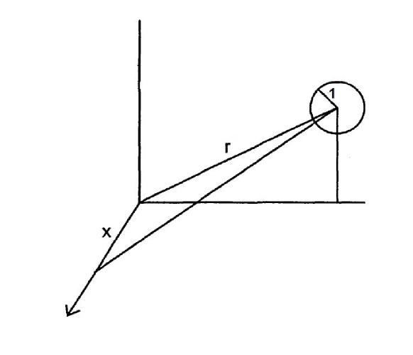
How far should an observer (a motorist) stand from an object (a circular road sign) so as to maximize its apparent size? Assume that the road is represented by the positive -axis and that the object is modeled by a disk of radius in the -plane, centered at a fixed distance from the origin (again ). The height of the observer is negligible (Figure 1). “Apparent size” is here quantified as the solid angle subtended by the disk at the observer’s eye. We wish to determine the vehicle location for which is maximized, i.e., the sign has greatest visual impact on the motorist (occupying the largest field of view).
This problem was solved in [4] via a Fourier-Legendre series approximation for . An exact formula, however, was mentioned by Maxwell [5] in 1873, explicitly given by Tallqvist [6] in 1931, and subsequently rediscovered several times [7, 8, 9, 10, 11, 12, 13, 14, 15, 16, 17, 18]:
where
is the complete elliptic integral of the first kind; and
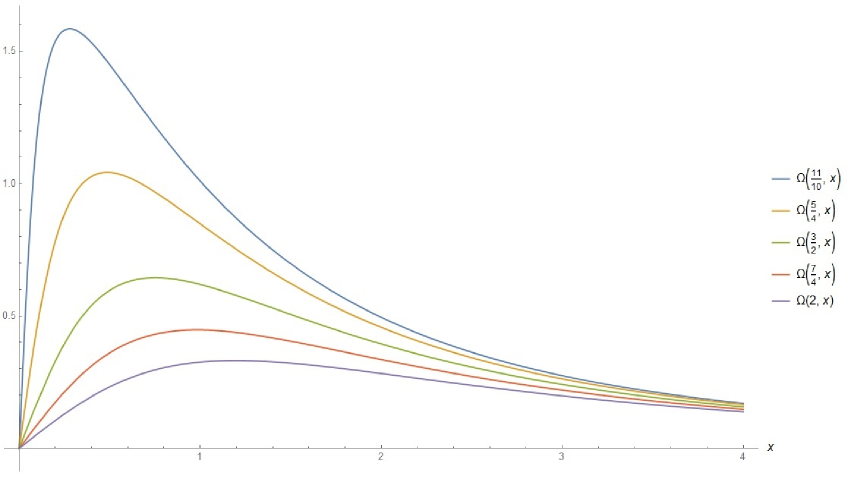
is the complete elliptic integral of the third kind (Figure 2). This formula enables precise asymptotics that could not be deduced in [4]. We have
as , which implies that
for large and which is an improvement on given earlier. We also have, for fixed ,
which plays a role in Koopman’s “inverse cube law of detection” from search theory [19, 20, 21].
2 Square versus Rectangular Billboards
The position of the circular sign in the preceding vignette was unspecified: it sufficed to require only that its center be at distance from the origin. Here, for a rectangular sign, we must further stipulate that its center possess -coordinates
that is, it lies on the diagonal line . Moreover, given that the rectangle has length and width , its vertices are assumed to be at
Letting the observer be at , we have [22, 23, 24, 25, 26]
and consequently
-
•
if and , then (a square)
-
•
if and , then
-
•
if and , then
This may be surprising to some readers: the rectangle of largest solid angle (with fixed observer and fixed center) need not be a square [3, 4]. The asymmetry (due to off-center location of observer relative to object) is responsible for this phenomena. For , the inequality is no longer satisfied, i.e., the billboard spills into the street. To talk of asymptotics as , we would perhaps wish to alter the position of the rectangle center.
3 Circular Deadbolt with Keyhole
The initial setting here is the -plane. Let the observer be at coordinate on the unit circle, centered at the origin. Let the object be the subinterval of the -axis. By the Law of Cosines, the angle subtended at the observer’s eye by the line segment is
If is uniformly distributed on the circle, then the first two moments of are
where
is the dilogarithm function [27]. Also, the probability density function of is
via standard techniques [28].
The final setting here is space. Let the observer be at coordinates on the unit sphere, centered at the origin. Let the object be the subinterval of the -axis. Note that
By the Law of Cosines, the angle subtended at the observer’s eye by the line segment is
If is uniformly distributed on the sphere, then the first two moments of are
and the probability density function of is
A closed-form expression for remains open. Substituting the line segment by a disk of diameter in the -plane, centered at the origin, also gives an unsolved problem.
4 Sphere around Framing Square
So far, we have addressed apparent size of lengths (of line segments) and areas (of planar regions). We conclude with apparent magnitude of angles (at the intersection of two lines).
Again, the setting is space. Let the observer be at coordinates on the unit sphere, centered at the origin. Call this point . Let , and , that is, a fixed angle of in the base plane. The apparent magnitude of relative to is the (dihedral) angle between normal vectors , to the triangular faces , respectively:
This formula is useful for simulation purposes. It’s best, however, to employ the spherical triangle and to recognize that the side opposite angle is the constant . From section 1.3 of [29], the conditional density for angle , given , is
In particular, a singularity exists at and
Let us change the vector from to . The side opposite angle is now the constant . It is known that [30]
but exact evaluation of
appears to be difficult.
Interested readers should examine [31] for an alternative derivation of the conditional mean , as well as a higher dimensional analog involving tetrahedra on (rather than triangles on ). No formula for the corresponding mean square is known here.
An expression for the solid angle subtended by a polygon can be used to approximate solid angles for arbitrary piecewise smooth closed curves [32, 33]. Our treatment of apparent size is based on Euclid (a visual cone of rays emanating from the eye); this system of thought is arguably inconsistent with the Renaissance theory of linear perspective [34, 35, 36, 37, 38]. We welcome correspondence on this topic, as an opportunity for deeper understanding.
5 Addendum
The “inverse cube law” mentioned at the end of the first vignette appears in other settings. We discuss this not with regard to spherical projection (definition of solid angle) but instead with respect to planar projection (image formed within a camera). Apparent size is quantified differently than before.
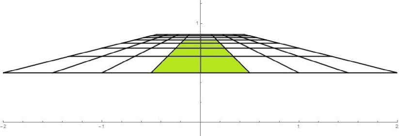
Consider an observer at in -space, surveying the integer lattice in the half -plane; according to this model, the observer does not see a uniform grid, but rather its projection into the -plane (Figure 3). The formula [39]
allows us to calculate the size of the trapezoid in the (green) center strip. We find
as .
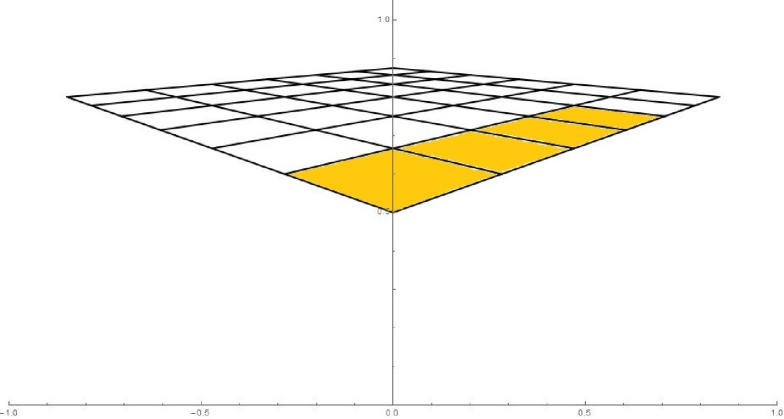
Consider instead an observer at in -space, surveying the lattice in the quarter -plane; the observer here sees a contrasting -projection (Figure 4). The formula
gives us the size of the quadrilateral in the (gold) right strip. We find here
as .
References
- [1] H. Dörrie, 100 Great Problems of Elementary Mathematics: Their History and Solution, Dover, 1965, pp. 369–370; MR0183598.
- [2] B. Letson and M. Schwartz, The Regiomontanus problem, Math. Mag. 90 (2017) 259–266; MR3706845.
- [3] A. Tan, The best viewing distance for highway signboards, Math. Spectrum 17 (1984/85) 33–35; summary in College Math. J. 16 (1985) 426.
- [4] I. S. Jones, The solid angle subtended by a circular disc with application to roadsigns, Int. J. Math. Educ. Sci. Technol. 27 (1996) 667–674.
- [5] J. C. Maxwell, A Treatise on Electricity and Magnetism, v. 2, 3 ed., Dover, 1954, p. 331.
- [6] Hj. Tallqvist, Tafeln zur scheinbaren Grösse des Kreises, Soc. Sci. Fennica, Commentationes Phys.-Math., v. 24, n. 5 (1931) 1–36.
- [7] M. W. Garrett, Solid angle subtended by a circular aperture, Rev. Sci. Instrum. 25 (1954) 1208–1211; cites Hj. Tallqvist.
- [8] A. V. Masket, Solid angle contour integrals, series, and tables, Rev. Sci. Instrum. 28 (1957) 191–197; cites P. A. Macklin.
- [9] M. Naito, A method of calculating the solid angle subtended by a circular aperture, J. Phys. Soc. Japan 12 (1957) 1122–1129; cites Hj. Tallqvist.
- [10] M. M. Agrest, M. Z. Maksimov and A. K. Khmelevskii, Determination of the solid angle subtended by a circular target at a point source, Zhur. Tekh. Fiziki 28 (1958) 1345–1347; Engl. transl. in Soviet Phys.-Tech. Phys. 3 (1958) 1249–1251.
- [11] F. Paxton, Solid angle calculation for a circular disk, Rev. Sci. Instrum. 30 (1959) 254–258.
- [12] A. V. Masket, Solid angle subtended by a circular disk, Rev. Sci. Instrum. 30 (1959) 950.
- [13] V. I. Lozgachev, The determination of solid angles, Zhur. Tekh. Fiziki 30 (1960) 1109–1114; Engl. transl. in Soviet Phys.-Tech. Phys. 5 (1961) 1039–1044.
- [14] R. E. Rothe, The solid angle at a point subtended by a circle, J. Franklin Instit. 287 (1969) 515–521.
- [15] V. A. Shelyuto, Exact analytic results for the solid angle in systems with axial symmetry, Z. Angew. Math. Phys. 40 (1989) 608–612; MR1008927.
- [16] M. J. Prata, Solid angle subtended by a cylindrical detector at a point source in terms of elliptic integrals, Radiat. Phys. Chem. 67 (2003) 599–603; arXiv:math-ph/0211061.
- [17] D. M. Timus, M. J. Prata, S. L. Kalla, M. I. Abbas, F. Oner and E. Galiano, Some further analytical results on the solid angle subtended at a point by a circular disk using elliptic integrals, Nucl. Instrum. Methods Phys. Res. A 580 (2007) 149–152.
- [18] J. T. Conway, Analytical solution for the solid angle subtended at any point by an ellipse via a point source radiation vector potential, Nucl. Instrum. Methods Phys. Res. A 614 (2010) 17–27.
- [19] B. O. Koopman, The theory of search. II. Target detection, Operations Research 4 (1956) 503–531; MR0090467.
- [20] L. D. Stone, Theory of Optimal Search, Academic Press, 1975, pp. 22–29; MR0439145.
- [21] L. D. Stone, J. O. Royset and A. R. Washburn, Optimal Search for Moving Targets, Springer-Verlag, 2016, pp. 13–19; MR3468906.
- [22] F. S. Crawford, Solid angle subtended by a finite rectangular counter Rev. Sci. Instrum. 24 (1953) 552–553.
- [23] A. Khadjavi, Calculation of solid angle subtended by rectangular apertures, J. Optical Soc. Amer. 58 (1968) 1417–1418.
- [24] H. Gotoh and H. Yagi, Solid angle subtended by a rectangular slit, Nucl. Instrum. Methods 96 (1971) 485–486.
- [25] J. Cook, Solid angle subtended by two rectangles, Nucl. Instrum. Methods 178 (1980) 561–564.
- [26] R. J. Mathar, Solid angle of a rectangular plate, unpublished note (2014), http://www2.mpia-hd.mpg.de/~mathar/public/.
- [27] S. R. Finch, Apéry’s constant, Mathematical Constants, Cambridge Univ. Press, 2003, pp. 40–53; MR2003519.
- [28] A. Papoulis, Probability, Random Variables, and Stochastic Processes, McGraw-Hill, 1965, pp. 125–127, 201–205; MR0176501.
- [29] S. R. Finch, Correlation between angle and side, arXiv:1012.0781.
- [30] Y. Maeda and H. Maehara, Observing an angle from various viewpoints, Discrete and Computational Geometry, Japanese Conference (JCDCG 2002), ed. J. Akiyama and M. Kano, Lect. Notes in Comp. Sci. 2866, Springer-Verlag, 2003, pp. 200–203; MR2097746.
- [31] Y. Maeda, Observing a solid angle from various viewpoints, Yokohama Math. J. 54 (2008) 155–160; MR2488281.
- [32] P. Olivier and D. Gagnon, Mathematical modeling of the solid angle function, part I: approximation in homogeneous medium, Optical Engin. 32 (1993) 2261–2265.
- [33] J. S. Asvestas and D. C. Englund, Computing the solid angle subtended by a planar figure, Optical Engin. 33 (1994) 4055–4059.
- [34] C. D. Brownson, Euclid’s Optics and its compatibility with linear perspective, Arch. Hist. Exact Sci. 24 (1981) 165–194; MR0632568.
- [35] W. R. Knorr, On the principle of linear perspective in Euclid’s Optics, Centaurus 34 (1991) 193–210; MR1166071.
- [36] W. R. Knorr, When circles don’t look like circles: an optical theorem in Euclid and Pappus, Arch. Hist. Exact Sci. 44 (1992) 287–329; MR1192853.
- [37] A. Jones, Pappus’ notes to Euclid’s Optics, Ancient & Medieval Traditions in the Exact Sciences, Proc. 1998 Stanford conf., CSLI Publ., 2000, pp. 49–58; MR1827652.
- [38] L. Catastini and F. Ghione, The geometry of sight: from Euclid’s Optics to Renaissance perspective, Matematica, Arte, Tecnologia, Cinema, ed. M. Emmer and M. Manaresi, Springer-Verlag Italia, 2002, pp. 53–66; MR2000794.
-
[39]
V. S. Nalwa, The basis of computer vision,
Mathematical Aspects of Artificial Intelligence, Proc. 1996 Orlando,
FL conf., ed. F. Hoffman, Proc. Sympos. Appl. Math. 55, Amer. Math. Soc.,
1998, pp. 139–174; MR1619608.
Steven Finch MIT Sloan School of Management Cambridge, MA, USA steven_finch@harvard.edu