Rigorously solvable model for the electrical conductivity of dispersions of hard-core–penetrable-shell particles and its applications

Abstract

We generalize the compact group approach to conducting systems to give a self-consistent analytical solution to the problem of the effective quasistatic electrical conductivity of macroscopically homogeneous and isotropic dispersions of hard-core–penetrable-shell particles. The shells are in general inhomogeneous and characterized by a radially-symmetrical, piecewise-continuous conductivity profile. The local value of the conductivity is determined by the shortest distance from the point of interest to the nearest particle. The effective conductivity is expressed in terms of the constituents’ conductivities and volume concentrations; the latter account for the statistical microstructure of the system. The theory effectively incorporates many-particle effects and is expected to be rigorous in the static limit. Using the well-tested statistical physics results for the shell volume concentration, this conclusion is backed up by mapping the theory on available 3D random resistor network simulations for hard spheres coated with fully penetrable concentric shells. Finally, the theory is shown to fit experimental data for real composite solid electrolytes. The fitting results indicate that the effect of enhanced electrical conduction is generally contributed to by several mechanisms. These are effectively taken into account through the shell conductivity profile.

I Introduction

The objectives of this paper are threefold: (1) to develop a homogenization theory for the effective quasistatic electrical conductivity $\sigma_{\rm eff}$ of macroscopically homogeneous and isotropic particulate substances and dispersions of particles with the core-shell morphology; (2) to test the theory by comparing its predictions with available results of random resistor network (RRN) simulations; and (3) to exemplify the applicability of the theory to real systems by processing experimental data for composite solid electrolytes (CSEs) prepared by dispersing fine insulating particles into matrix ionic conductors.

The indicated class of composites attracts a special attention due to nontrivial behavior of their $\sigma_{\rm eff}$. Through the addition of filler particles (for instance, alumina particles, with electrical conductivity $\sigma_{1}\sim 10^{-14}\,{\rm{S/cm}}$) to matrix ionic conductors (such as polycrystalline metal halides, whose typical electrical conductivities $\sigma_{0}\sim 10^{-10}\div 10^{-5}\,{\rm{S/cm}}$), $\sigma_{\rm{eff}}$ of the resulting CSEs can be increased dramatically, by one to three orders of magnitude as compared to $\sigma_{0}$. This effect is called enhanced ionic conduction. Since its discovery by Liang Liang1973 in polycrystalline lithium iodide containing alumina particles, it has been observed in dozens of CSEs (for a detailed bibliography, see reviews Wagner1980 ; Takahashi1989 ; Dudney1989 ; Maier1995 ; Agrawal1999 ; Uvarov2011 ; Kharton2011 ; Gao2016 ) and composite polymer-based electrolytes (Knauth2008 ; Sequeira2010 ) to make those promising materials for electrolytic applications.

Experiment also reveals that the maximum conduction enhancement usually occurs as the filler volume concentration $c$ reaches values in between 0.1 and 0.4. It is followed by a decrease in $\sigma_{\rm{eff}}$ as $c$ is further increased. Such a nonmonotonic dependence of $\sigma_{\rm{eff}}$ upon $c$ is a challenging problem for homogenization theory, since the existing approaches to two-phase systems, such as the classical Maxwell-Garnet Maxwell1873 ; Maxwell1904 and Bruggeman Bruggeman1935 ; Landauer1952 mixing rules, their numerous modifications (see Bohren1983 ; Bergman1992 ; Sihvola1999 ; Tsang2001 ; Torquato2013 ; Milton2004 ), cluster expansions Torquato1984 ; Torquato1985b for dispersions of spheres with arbitrary degree of impenetrability, their extensions Torquato1985 with the Padé approximant technique, and systematic simulations MyroshnychenkoPRE2005 ; MyroshnychenkoJAP2005 ; Myroshnychenko2008 ; Myroshnychenko2010 of random 2D systems of hard-core–penetrable-shell discs by combining Monte Carlo algorithms and finite element calculations do not exhibit it. The reason is that two-phase models oversimplify the actual microstructure of CSEs and disregard the processes involved.

A typical way out is to model a CSE as a three-phase system and determine $\sigma_{\rm{eff}}$ by solving a pertinent homogenization problem. The solution is expressed in terms of the geometric and electric parameters of the phases. These parameters are estimated so as to incorporate the relevant physical effects and account for the observed behavior of $\sigma_{\rm eff}$. Several classes of such models have been proposed.

(i) Cubic lattices of cubic insulators surrounded by highly conductive layers and embedded in a conductive material Wang1979 ; Jiang1995a ; Jiang1995b . The arrangement of particles on a simple cubic lattice makes it possible to represent the system with a resistor network and to calculate $\sigma_{\rm eff}$ for the entire range of $c$. The results suggest that the conductivity in the layer outside each particle may have a maximum at certain distance away from the surface.

(ii) Three-component resistor models with a matrix represented by normally conducting bonds, the inert randomly distributed (quadratic or cubic) particles by insulating bonds, and the interface region by highly conducting bonds Bunde1985 ; Roman1986 ; Blender1987 . The models are solved by Monte Carlo simulations or a position-space reorganization technique and exhibit two threshold concentrations of the insulating material. One corresponds to the onset of interface percolation and the second one to a conductor-insulator transition. The effective medium and continuum percolation approaches to these models are discussed in Rojo1988 and Roman1987 ; Roman1990 , respectively.

(iii) Random three-phase dispersions of spherical particles comprising hard cores coated with concentric shells, either hard or penetrable (see Fig. 1), of potentially higher conductivity. Such core-shell models better suit the physical conditions in CSEs, but are harder to analyze. Analytical studies, such as Stoneham1979 ; Brailsford1986 ; Nan1991L ; Nan1991 ; Nan1993 ; Wiec1994 , of them are usually limited to the case of hard shells, involve a sequence of one-particle approximations, and repeatedly use the Maxwell-Garnet Maxwell1873 ; Maxwell1904 or/and Bruggeman Bruggeman1935 ; Landauer1952 mixing rules. The case of penetrable shells has been attacked through RRN simulations, such as Siekierski2005 ; Siekierski2006 ; Siekierski2007 for mono- and Kalnaus2011 for polysized particles. The essential details of these core-shell model results are scrutinized in Sec. VIII.

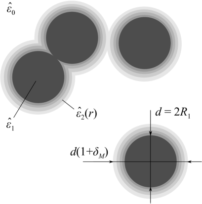
Figure 1: The model under consideration. Each dispersed particle consists of a spherical hard core (shown black) with diameter $d=2R_{1}$ and complex permittivity $\hat{\varepsilon}_{1}$. The core is coated with an isotropic (generally inhomogeneous) penetrable concentric shell (graded gray) with outer diameter $D=d(1+\delta_{M})$, relative thickness $\delta_{M}=(D-d)/d$, and complex permittivity profile $\hat{\varepsilon}_{2}=\hat{\varepsilon}_{2}(r)$. The particles are embedded in a uniform matrix (white) with complex permittivity $\hat{\varepsilon}_{0}$. All the permittivities have form (5). The local value of the permittivity is determined by the shortest distance from the point of interest to the nearest particle.

In what follows, we derive a self-consistent analytic many-particle solution for $\sigma_{\rm eff}$ of macroscopically homogeneous and isotropic 3D model dispersions of hard-core–penetrable-shell spheres, the shells being, in the general case, electrically inhomogeneous and characterized by radially-symmetrical, piecewise-continuous conductivity profiles (see Fig. 1 for the details of the model). The desired $\sigma_{\rm eff}$ is a functional of the constituents’ conductivities and volume concentrations that satisfies a certain integral relation, rigorous in the static limit. The volume concentrations account for the statistical microstructure of the system.

The derivation is carried out using the compact groups approach (CGA) Sushko2007 ; Sushko2009CompGroups ; Sushko2009AnisPart ; Sushko2017 . It was originally designed to efficiently take into account many-particle polarization and correlation effects, without an in-depth modeling of those, in concentrated dielectric dispersions. In this paper, elaborating its statistical-averaging version, we (1) generalize the CGA to conducting systems whose constituents have complex permittivities with first-order poles at frequency $\omega=0$; (2) scrutinize, for such systems, the passage to the (quasi)static limit $\omega\to 0$ in all terms of the iterative series for the averaged electric field and current; (3) bring new arguments, not restricted to dielectric systems, for the internally-consistent closure of the homogenization procedure and determination of the complex permittivity of the auxiliary host matrix; and (4) propose a technique for dealing with inhomogeneous overlapping regions.

Using the well-tested statistical physics results Rikvold85 ; Lee1988 ; Rottereau2003 for the shell volume concentration, we then validate the solution obtained by mapping it onto the entire set of available 3D random resistor network simulation data Siekierski2005 ; Siekierski2006 ; Siekierski2007 for dispersions of hard spheres coated with fully penetrable (electrically uniform or inhomogeneous) concentric shells. The solution is capable of recovering all of these data in the entire ranges of $c$ simulated. To our best knowledge, no such an analytic solution has been offered so far even for the simplest case of uniform shells with their conductivity being equal to that of the cores.

Finally, we apply the model to real CSEs. The results of processing experimental data Liang1973 clearly indicate that the concept of inhomogeneous penetrable shells provides an efficient way for describing the net effect on $\sigma_{\rm eff}$ by different mechanisms. The latter may contribute most significantly in different ranges of $c$. If so, they are accounted for by different parts in the model shell conductivity profile. This fact opens new opportunities for scrutinizing the physics of processes in real composites, which is of crucial importance in the situation where the consensus of opinions regarding the nature of ionic conduction enhancement in various composites has not been reached as yet Agrawal1999 ; Uvarov2011 ; Kharton2011 ; Gao2016 .

The paper is arranged as follows. Some basic equations and definitions of macroscopic electrodynamics for media with complex permittivities of the constituents are recalled in Sec. II. With those in mind, the CGA is generalized in Sec. III to the problem of the effective quasistatic complex permittivity $\hat{\varepsilon}_{\rm{eff}}$ of macroscopically homogeneous and isotropic dispersions. The governing equation for $\hat{\varepsilon}_{\rm{eff}}$ is expressed in terms of the statistical moments $\langle\left(\delta\hat{\varepsilon}({\rm{\bf r}})\right)^{s}\rangle$ for the local deviations of the permittivity distribution in the dispersion from the complex permittivity $\hat{\varepsilon}_{\rm{f}}$ of the host in the auxiliary system. By requiring that the CGA and boundary conditions Sillars1937 for complex electric fields be compatible, $\hat{\varepsilon}_{\rm{f}}$ is determined in Sec. IV. The calculations of $\langle\left(\delta\hat{\varepsilon}({\rm{\bf r}})\right)^{s}\rangle$ for dispersions of isotropic core-shell particles with electrically homogeneous and inhomogeneous shells are performed in Secs. V and VI, respectively. The resultant equations for $\sigma_{\rm eff}$ are presented in Sec. VII. Their validity is shown in Sec. VIII by mapping their solutions onto extensive RRN simulation data Siekierski2005 ; Siekierski2007 ; Siekierski2006 . The applicability of the theory to real ${\rm LiI/Al_{2}O_{3}}$ CSEs Liang1973 is discussed in Sec. IX. The main results of the paper are summarized in Sec. X.

II Basic equations and definitions

Consider the electromagnetic field caused in a nonmagnetic heterogeneous medium by time-harmonic ($\sim e^{-i\omega t}$, $i$ being the imaginary unit) probing radiation whose working frequencies $\omega$ are sufficiently small to neglect any dielectric relaxation phenomena. The relevant frequency-domain Maxwell’s macroscopic equations, written in the Gaussian units, have the form

$${}{\rm div}\,{\bf D}=4\pi\rho,\quad{\rm div}\,{\bf H}=0,$$ (1)

$${}{\rm curl}\,{\bf E}=i\frac{\omega}{c}\,{\bf H},\quad{\rm curl}\,{\bf H}=\frac{4\pi}{c}\,{\bf j}-i\frac{\omega}{c}\,{\bf D},$$ (2)

where ${\bf E}$, ${\bf D}$, ${\bf H}$, $\rho$, and ${\bf j}$ are the amplitude distributions of the electric field, electric displacement, magnetic field, free charge density, and free current density, respectively, and $c$ is the speed of light in vacuum. The densities $\rho$ and ${\bf j}$ are related by the continuity equation

$${}-i\omega\rho+{\rm div}\,{\bf j}=0.$$ (3)

Assuming the standard linear constitutive equations

$${}{\bf D}=\varepsilon{\bf E},\quad{\bf j}=\sigma{\bf E},$$ (4)

where $\varepsilon=\varepsilon({\bf r})$ and $\sigma=\sigma({\bf r})$ are the local (real) dielectric constant and electrical conductivity in the medium, one can introduce the quasistatic complex permittivity

$${}{\hat{\varepsilon}}=\varepsilon+i\frac{4\pi\sigma}{\omega}$$ (5)

of the medium to obtain from Eqs. (1)–(4) the equation for the quasistatic electric field distribution

$$\Delta{\bf E}+k^{2}_{0}\hat{\varepsilon}\,{\bf E}-{\rm grad}\,{\rm div}{\textbf{E}}=0,$$ (6)

where $k_{0}=\omega/c$ is the magnitude of the wave vector ${\bf k}_{0}$ of the incident field in vacuum, and define the complex current density

$${}{\bf J}=-i\frac{\omega}{4\pi}\,{\hat{\varepsilon}}\,{\bf E},\quad{\rm div}\,{\bf J}=0.$$ (7)

The first Eq. (7) reduces in the static limit ($\omega\to 0$) to Ohm’s law, given by the second Eq. (4).

III Compact group approach to homogenization of conducting systems

The main points of this approach in application to macroscopically homogeneous and isotropic nonconducting systems are discussed in detail in Sushko2007 ; Sushko2009CompGroups ; Sushko2009AnisPart ; Sushko2017 . Here, closely following the summary in Sushko2017 , we outline a generalization of the approach to macroscopically homogeneous and isotropic dispersions $\cal{D}$ comprising conducting constituents, such as conducting dielectrics or imperfectly insulating materials. In view of the Kramers-Kronig relations in the linear response theory, we assume that for a given $\cal{D}$, the complex permittivities of all the constituents have structure (5), where $\varepsilon$ and $\sigma$ are in general piecewise-continuous and bounded real functions of spacial coordinates; and that its $\hat{\varepsilon}_{\rm eff}=\varepsilon_{\rm eff}+i4\pi\sigma_{\rm eff}/\omega$ can be calculated based upon the following suggestions:

(1) $\cal{D}$ is equivalent, in its response to a long-wavelength probing field ($\omega\to 0$), to an auxiliary system $\cal{S}$ prepared by embedding the constituents (particles and matrix) of $\cal{D}$ into a uniform host (perhaps, imagined) $\cal{M}$ with some permittivity $\hat{\varepsilon}_{\rm f}$.

(2) $\cal{S}$ can be viewed as a set of compact groups of both particles and regions occupied by the real matrix. The compact groups are defined as macroscopic regions whose typical sizes $d$ are much smaller than the wavelength $\lambda$ of probing radiation in $\cal{M}$, but which yet include sufficiently large numbers $N$ of particles to remain macroscopic and retain the properties of the entire $\cal{S}$.

(3) The complex permittivity distribution in $\cal{S}$ is

$$\hat{\varepsilon}({\bf{r}})=\hat{\varepsilon}_{\rm f}+\delta\hat{\varepsilon}({\bf{r}})$$ (8)

where $\delta\hat{\varepsilon}(\bf{r})$ is the contribution from a compact group located at point $\bf{r}$. The explicit form of $\delta{\hat{\varepsilon}}({\bf{r}})$ is modeled according to the geometrical and electrical parameters of $\cal{D}$’s constituents.

(4) $\hat{\varepsilon}_{\rm{eff}}$ can be found as the proportionality coefficient in the relation

$$\langle{\bf{J}}({\bf{r}})\rangle=-i\frac{\omega}{4\pi}\langle\hat{\varepsilon}({\bf{r}}){\bf{E}}({\bf{r}})\rangle=-i\frac{\omega}{4\pi}\hat{\varepsilon}_{\rm eff}\langle{\bf{E}}({\bf{r}})\rangle,$$ (9)

where ${\bf{J}}({\bf{r}})$ and ${\bf{E}}({\bf{r}})$ are the local values of the complex current and electric field, respectively, and the angle brackets stand for the ensemble averaging. In the static limit, provided $\lim_{\omega\to 0}\omega{\varepsilon}({\bf{r}})=0$ and ${\bf{E}}({\bf{r}})$ is real-valued, Eq. (9) reduces to the common definition Bergman1992 ; Sihvola1999 ; Torquato2013 of the effective conductivity:

$$\langle\bf{j}({\bf{r}})\rangle=\langle\sigma({\bf{r}}){\bf{E}}({\bf{r}})\rangle=\sigma_{\rm eff}\langle{\bf{E}}({\bf{r}})\rangle.$$ (10)

(5) The electric field distribution $\textbf{E}(\textbf{r})$ in $\cal{S}$ obeys the equation

$$\Delta{\bf E}+k_{0}^{2}\hat{\varepsilon}_{\rm f}{\bf E}-{\rm grad}\,{\rm div}{\textbf{E}}=-k_{0}^{2}\delta\hat{\varepsilon}{\bf E},$$ (11)

which directly follows from Eqs. (6) and (8). The equivalent integral equation is

$${\rm{\bf E}}({\rm{\bf r}})={\rm{\bf E}}_{0}({\rm{\bf r}})-{\int\limits_{V}{d{\rm{\bf{r}^{\prime}}}\,}}{\rm T}(|{\rm{\bf r}}-{\rm{\bf{r}^{\prime}}}|)k_{0}^{2}\delta\hat{\varepsilon}({\rm{\bf{r}^{\prime}}})\,{\rm{\bf E}}({\rm{\bf{r}^{\prime}}}),$$ (12)

where ${\rm{\bf E}}_{0}({\rm{\bf r}})={\rm{\bf E}}_{0}\exp(i\,{\rm{\bf k}}\cdot{\rm{\bf r}})$, ${\rm\bf{E}_{0}}$, and ${\bf k}={\hat{\varepsilon}_{\rm f}}^{1/2}{\rm{\bf k}_{0}}$ (with ${\rm{Im}}\,{\hat{\varepsilon}_{\rm f}}^{1/2}\geq 0$) are, respectively, the incident wave field, its amplitude, and its wave vector in ${\cal M}$, and ${\rm T}(r)$ is the Green’s tensor of Eq. (11).

(6) The formal solution for ${\bf{E}}({\bf{r}})$ and those for ${\bf{J}}({\bf{r}})$, $\langle{\bf{E}}({\bf{r}})\rangle$, and $\langle{\bf{J}}({\bf{r}})\rangle$ are representable in the form of infinite iterative series. For systems whose constituents have the permittivities of form (5), the functions $k_{0}^{2}\delta\hat{\varepsilon}({\rm{\bf r}})$ in the integrands and also the function $\omega\hat{\varepsilon}({\rm{\bf r}})$ remain bounded even at $\omega\to 0$, where $|{\rm{\bf k}}|\to 0$ as well. Mathematically, the situation is identical to that for nonconducting systems and can be treated analogously. Namely, in the iterative series for $\langle{\bf{E}}({\bf{r}})\rangle$ and $\langle{\bf{J}}({\bf{r}})\rangle$, each ${\rm T}$ under the integral sign is replaced by its decomposition ${\widetilde{\rm T}}$, derived for a spherical exclusion volume of radius $a\to 0$, into a Dirac delta function singular part and a principal value part Ryzhov1965 ; Weiglhofer1989 :

$${\widetilde{T}}_{\alpha\beta}({\rm{\bf r}})=\frac{1}{3k^{2}}\delta_{\alpha\beta}\delta({\rm{\bf r}})\,e^{ikr}+\frac{1}{4\pi k^{2}}\left(\frac{1}{r^{3}}-\frac{ik}{r^{2}}\right)$$

$$\times\left(\delta_{\alpha\beta}-3e_{\alpha}e_{\beta}\right)\,e^{ikr}-\frac{1}{4\pi r}\left({\delta_{\alpha\beta}-e_{\alpha}e_{\beta}}\right)\,e^{ikr},$$ (13)

where $\delta({\bf r})$ is the Dirac delta function, $\delta_{\alpha\beta}$ is the Kronecker delta, and $e_{\alpha}$ is the $\alpha$-component of the unit vector ${\bf e}={\bf r}/r$. The contributions to $\langle{\rm{\bf{E}}({\bf r})}\rangle$ made by the subseries containing, in their integrands, the principal value parts are estimated to be of the order $|\hat{\varepsilon}_{\rm f}|k_{0}^{2}L^{3}/d$, at most Sushko2007 , as compared to those made by the subseries with only the Dirac delta function parts. For a finite typical linear size $L$ of the system, the former can be decreased below any preset value by taking a sufficiently small $k_{0}$. So, passing to the limit $\omega\to 0$ and formally replacing each ${\widetilde{\rm T}}$ in the integrals for $\langle{\bf{E}}({\bf{r}})\rangle$ and $\langle{\bf{J}}({\bf{r}})\rangle$ by its Delta function part, we obtain

$$\lim_{\omega\to 0}\left\langle{\mathbf{E}}({\mathbf{r}})\right\rangle=\lim_{\omega\to 0}\left[1+\langle\hat{Q}({\mathbf{r}})\rangle\right]{{\mathbf{E}}_{0}},$$ (14)

$$\lim_{\omega\to 0}\left\langle{\mathbf{J}}({\mathbf{r}})\right\rangle=-i\lim_{\omega\to 0}\frac{\omega\hat{\varepsilon}_{\rm{f}}}{4\pi}\left[1-2\langle\hat{Q}({\mathbf{r}})\rangle\right]{{\mathbf{E}}_{0}},$$ (15)

where

$$\hat{Q}({\mathbf{r}})\equiv\sum\limits_{s=1}^{\infty}\left(-\frac{1}{3\hat{\varepsilon}_{\rm{f}}}\right)^{s}(\delta\hat{\varepsilon}({\mathbf{r}}))^{s}.$$ (16)

(7) The above results can be obtained without resort to iterative series. Indeed, it follows from Eq. (III) that

$$\lim_{\omega\to 0}k_{0}^{2}\hat{\varepsilon}_{\rm f}{\widetilde{T}}_{\alpha\beta}({\rm{\bf r}})=\tau^{(1)}_{\alpha\beta}+\tau^{(2)}_{\alpha\beta},$$ (17)

where

$$\tau^{(1)}_{\alpha\beta}=\frac{1}{3}\,\delta_{\alpha\beta}\delta({\rm{\bf r}}),\quad\tau^{(2)}_{\alpha\beta}=\frac{{\delta_{\alpha\beta}-3e_{\alpha}e_{\beta}}}{4\pi r^{3}}.$$ (18)

Substituting Eqs. (17) and (18) into Eq. (12), making simple algebraic manipulations and statistical averaging, and implying that $\omega\to 0$, we obtain

$$\begin{split}\langle\mathbf{E}&(\mathbf{r})\rangle=\left\langle\frac{3\hat{\varepsilon}_{\rm f}}{3\hat{\varepsilon}_{\rm f}+\delta\hat{\varepsilon}({\bf r})}\right\rangle\mathbf{E}_{0}\\ &-3\int\limits_{V}{d{\mathbf{r}}^{\prime}}{\rm{\tau}^{(2)}(|{\bf r}-{\bf r}^{\prime}|)\left\langle\frac{\delta\hat{\varepsilon}({\mathbf{r}}^{\prime})}{3\hat{\varepsilon}_{\rm f}+\delta\hat{\varepsilon}({\bf r})}{\mathbf{E}}({\mathbf{r}}^{\prime})\right\rangle},\end{split}$$ (19)

$$\begin{split}\langle\mathbf{J}&(\mathbf{r})\rangle=-i\frac{\omega}{4\pi}\,\hat{\varepsilon}_{\rm f}\left[1+2\left\langle\frac{\delta\hat{\varepsilon}({\bf r})}{3\hat{\varepsilon}_{\rm f}+\delta\hat{\varepsilon}({\bf r})}\right\rangle\right]\mathbf{E}_{0}\\ &+i\frac{3}{4\pi}\,\int\limits_{V}{d{\mathbf{r}}^{\prime}}{\rm{\tau}^{(2)}(|{\bf r}-{\bf r}^{\prime}|)\left\langle\frac{\omega\,\hat{\varepsilon}({\bf r})\,\delta\hat{\varepsilon}({\mathbf{r}}^{\prime})}{3\hat{\varepsilon}_{\rm f}+\delta\hat{\varepsilon}({\bf r})}{\mathbf{E}}({\mathbf{r}}^{\prime})\right\rangle}.\end{split}$$ (20)

For macroscopically isotropic and homogeneous systems, two-point statistical averages depend only on $|{\bf r}-{\bf r}^{\prime}|$. Due to this symmetry and because of a special form of the angular dependence of $\tau_{\alpha\beta}^{(2)}$, the integrals in Eqs. (19) and (20) vanish. Finally, viewing the expressions in the angle brackets as the sums of infinite geometric series, we arrive at Eqs. (14)–(16).

This consideration is very similar to that used in the strong-property-fluctuation theory (SPFT) Tsang2001 ; Ryzhov1965 ; Ryzhov1970 ; Tamoikin1971 ; Tsang1981 ; Zhuck1994 ; Michel1995 ; Mackay2000 ; Mackay2001 . However, our theory gives another interpretation to $\delta\hat{\varepsilon}({\rm{\bf{r}}})$, appeals to the macroscopic symmetry of the entire system instead of the symmetry of correlation functions, and postulates no condition on the stochastic field $\hat{\xi}({\bf r})=[\hat{\varepsilon}({\bf r})-\hat{\varepsilon}_{\rm f}]/[2\hat{\varepsilon}_{\rm f}+\hat{\varepsilon}({\bf r})]=\delta\hat{\varepsilon}({\bf r})/[3\hat{\varepsilon}_{\rm f}+\delta\hat{\varepsilon}({\bf r})]$ in order to improve the convergence of the iteration procedure and decide on the value of $\hat{\varepsilon}_{\rm f}$. Once the latter is determined, the analysis of $\hat{\varepsilon}_{\rm eff}$ reduces to modeling $\delta\hat{\varepsilon}({\rm{\bf r}})$, calculating its moments $\langle\left({\delta\hat{\varepsilon}({\rm{\bf r}})}\right)^{s}\rangle$, and finding their sum in Eqs.  (14) and (15).

IV Determination of $\hat{\varepsilon}_{\rm f}$

If the permittivities of the constituents, that of $\cal{M}$, and $\hat{\varepsilon}_{\rm eff}$ have at $\omega\to 0$ the structure (5), then, at least in this limit, it is the Bruggeman-type of homogenization $\hat{\varepsilon}_{\rm f}=\hat{\varepsilon}_{\rm eff}$ that is compatible with the formalism of the CGA and definition (9). To prove this statement, we first remind that ${\bf E}_{0}$ is the amplitude of the probing electric field in the uniform fictitious matrix of permittivity $\hat{\varepsilon}_{\text{f}}$, and $\left\langle{\mathbf{E}}({\mathbf{r}})\right\rangle$ is the effective electric field in the homogenized dispersion of permittivity $\hat{\varepsilon}_{\rm eff}$, caused by the same probing field. Next, we recall the boundary condition Sillars1937

$$\hat{\varepsilon}_{1}E_{1n}=\hat{\varepsilon}_{2}E_{2n}$$

for the normal components of complex electric fields at the surface between two conducting dielectrics (or imperfectly insulating materials) with permittivities of type (5). For the surface between the fictitious matrix and the homogenized dispersion, it gives

$$\hat{\varepsilon}_{\rm f}{\mathbf{E}}_{0n}=\hat{\varepsilon}_{\rm eff}\left\langle{\mathbf{E}}({\mathbf{r}})\right\rangle_{n}.$$ (21)

This relation, Eq. (9), and Eqs. (14)–(16) yield, at $\omega\to 0$, the system of equations

$$\begin{gathered}\hat{\varepsilon}_{\rm f}=\hat{\varepsilon}_{\rm eff}\left(1+\langle\hat{Q}\rangle\right),\\ \hat{\varepsilon}_{\rm f}\left(1-2\langle\hat{Q}\rangle\right)=\hat{\varepsilon}_{\rm eff}\left(1+\langle\hat{Q}\rangle\right).\end{gathered}$$ (22)

Since $\hat{\varepsilon}_{\rm f}\neq 0$, it follows immediately that

$$\hat{\varepsilon}_{\rm f}=\hat{\varepsilon}_{\rm eff}$$ (23)

and, for this $\hat{\varepsilon}_{\rm f}$,

$$\langle\hat{Q}({\mathbf{r}})\rangle=0.$$ (24)

The latter is the desired governing equation for $\hat{\varepsilon}_{\rm eff}$. It is valid in the limit $\omega\to 0$.

It can be shown Sushko2017 that for two-constituent systems (say, hard spheres embedded in a uniform host), Eqs. (23) and (24) reproduce the Bruggeman result Bruggeman1935 ; Landauer1952 ; Ross2005 derived within the assumption that spherical inclusions of all constituent materials are placed in the effective medium. The same Eqs. (23), (24), and Bruggeman result also follow, in the quasistatic limit, from the SPFT Tsang1981 for hard spheres where the condition $\langle\hat{\xi}({\bf r})\rangle=0$ is imposed to eliminate the secular terms and the bilocal approximation is implemented for a special case of the spherically symmetric two-point correlation function $\langle\hat{\xi}({\bf r})\hat{\xi}({\bf r^{\prime}})\rangle$.

V Statistical moments $\langle\left(\delta\hat{\varepsilon}({\rm{\bf r}})\right)^{s}\rangle$

We consider a dispersion of $N$ spherically symmetrical core-shell particles embedded into a uniform matrix. Suppose that the local permittivity value at a point $\bf r$ within the dispersion is determined by the distance $l\equiv\min\limits_{1\leq a\leq N}|{\bf r}-{\bf r}_{a}|$ from $\bf r$ to the center of the nearest ball as

$$\hat{\varepsilon}({\bf r})=\begin{cases}\hat{\varepsilon}_{1}&{\text{if}}\quad\,\,l<R_{1},\\ \hat{\varepsilon}_{2}&{\text{if}}\quad R_{1}<l<R_{2},\\ \hat{\varepsilon}_{0}&{\text{if}}\quad\,\,l>R_{2}.\end{cases}$$ (25)

Here $R_{1}$ is the radius of the core of complex permittivity $\hat{\varepsilon}_{1}$, $R_{2}$ is the outer radius of the shell of complex permittivity $\hat{\varepsilon}_{2}$, and $\hat{\varepsilon}_{0}$ is the complex permittivity of the matrix. Within the CGA Sushko2007 ; Sushko2009CompGroups ; Sushko2009AnisPart ; Sushko2017 , such a system can be modelled as follows.

Let $\theta(x)$ be the Heaviside step function and $\chi_{a}^{(q)}({\bf r})=\theta\left(R_{q}-|{\bf r}-{\bf r}_{a}|\right)$ ($q=0,1,2$) be the characteristic functions of balls centered at point ${\bf r}_{a}$ and having radii $R_{q}$. Suggesting that $R_{1}<R_{2}<R_{0}$ and allowing the balls to overlap, consider the complex permittivity distribution of form (8) with

$$\delta\hat{\varepsilon}({\bf r}) = \Pi_{1}({\bf r})\Delta\hat{\varepsilon}_{1}+\left[\Pi_{2}({\bf r})-\Pi_{1}({\bf r})\right]\Delta\hat{\varepsilon}_{2}$$ (26)

$$+\left[\Pi_{0}({\bf r})-\Pi_{2}({\bf r})\right]\Delta\hat{\varepsilon}_{0},$$

where $\Delta\hat{\varepsilon}_{q}=\hat{\varepsilon}_{q}-\hat{\varepsilon}_{\rm f}$, and each

$$\Pi_{q}({\bf r})=1-\prod\limits_{a=1}^{N}\left(1-\chi_{a}^{(q)}\left({\bf r}\right)\right)$$ (27)

is the characteristic (indicator) function of the collection of balls of radius $R_{q}$. In the limit $R_{0}\to\infty$, $\Pi_{0}({\bf r})\to 1$ and Eq. (26) leads to the model permittivity distribution (25) for a dispersion of penetrable core-shell particles embedded into a uniform matrix of permittivity $\hat{\varepsilon}_{0}$. Note that $R_{0}$ is a convenient auxiliary parameter (having nothing to do with the physical geometry) which is used for the host matrix to be introduced within the same formal algorithm as the other constituents are. The characteristic function of the entire region occupied by the substance of permittivity $\hat{\varepsilon_{q}}$ in this dispersion is given by the coefficient function in front of the corresponding $\Delta\hat{\varepsilon}_{q}$. It is readily verified that the characteristic functions of regions with different permittivities are mutually orthogonal.

Further, we limit ourselves to the case of particles with hard cores. Then $\chi_{a}^{(1)}({\bf r})\chi_{b}^{(1)}({\bf r})=\delta_{ab}\chi_{a}^{(1)}({\bf r}),$ where $\delta_{ab}$ is the Kronecker delta, and $\Pi_{1}({\bf r})$ reduces to

$$\Pi_{1}({\bf r})=\sum\limits_{a=1}^{N}\chi_{a}^{(1)}\left({\bf r}\right),$$ (28)

with the additional restriction $|{\bf r}_{a}-{\bf r}_{b}|\geq 2R_{1}$ on the locations of any two balls.

For a macroscopically homogeneous and isotropic system

$$\left\langle\sum\limits_{a=1}^{N}\chi_{a}^{(1)}\left({\bf r}\right)\right\rangle=c,$$

where $c$ is the volume concentration of the hard cores. In view of this fact and the mutual orthogonality of the characteristic functions of regions with different permittivities, the moments of the function (26) can be represented in the limit $R_{0}\to\infty$ as

$$\langle\left[\delta\hat{\varepsilon}({\bf r})\right]^{s}\rangle = c\left(\Delta\hat{\varepsilon}_{1}\right)^{s}+\left(\phi(c,\delta)-c\right)\left(\Delta\hat{\varepsilon}_{2}\right)^{s}$$ (29)

$$+\left(1-\phi(c,\delta)\right)\left(\Delta\hat{\varepsilon}_{0}\right)^{s},$$

where

$$\phi(c,\delta) \equiv \left\langle\Pi_{2}({\bf r})\right\rangle=\left\langle\left[1-\prod\limits_{a=1}^{N}\left(1-\chi_{a}^{(2)}\left({\bf r}\right)\right)\right]\right\rangle$$

$$= \left\langle\sum\limits_{1\leq a\leq N}{\chi}_{a}^{\,(2)}\left({\bf r}\right)-\sum\limits_{1\leq a<b\leq N}{\chi}_{a}^{\,(2)}\left({\bf r}\right){\chi}_{b}^{\,(2)}\left({\bf r}\right)\right.$$

$$+\left.\sum\limits_{1\leq a<b<c\leq N}{\chi}_{a}^{\,(2)}\left({\bf r}\right){\chi}_{b}^{\,(2)}\left({\bf r}\right){\chi}_{c}^{\,(2)}\left({\bf r}\right)-\ldots\right\rangle$$

is the effective volume concentration of hard-core–penetrable-shell particles Torquato2013 . Besides $c$, it depends on the relative thickness of the shell $\delta=\left(R_{2}-R_{1}\right)/R_{1}$; in particular, $\phi(c,0)=c$. The averaged values of the sums in Eq. (LABEL:eq:effectiveconcentration) are calculated using the partial distribution functions $F_{s}({\bf r}_{1},{\bf r}_{2},\ldots,{\bf r}_{s})$ for the system under consideration.

For hard-core–hard-shell particles Eq. (LABEL:eq:effectiveconcentration) gives

$$\phi(c,\delta)=c(1+\delta)^{3}.$$ (31)

VI The Case of Inhomogeneous Isotropic Shells

To extend the results of Sec. V to dispersions of spherically symmetrical particles with hard cores and adjacent inhomogeneous penetrable shells, we begin with the situation where each shell consists of $M$ concentric spherical layers with outer radii $R_{2,m}$ (grouped in the order of increasing magnitude) and constant dielectric permittivities $\hat{\varepsilon}_{2,m}$, $m=1,2,\dots,M$. Next, we suggest that the local permittivity distribution within the dispersion is given by this law, generalizing Eq. (25):

$$\hat{\varepsilon}({\bf r})=\begin{cases}\hat{\varepsilon}_{1}&{\text{if}}\quad\,\,l<R_{1},\\ \hat{\varepsilon}_{2,1}&{\text{if}}\quad R_{1}<l<R_{2,1},\\ \hat{\varepsilon}_{2,m}&{\text{if}}\quad R_{2,m-1}<l<R_{2,m},\,2\leq m\leq M,\\ \hat{\varepsilon}_{0}&{\text{if}}\quad\,\,l>R_{2,M}.\end{cases}$$ (32)

Let $\chi_{a}^{(2,m)}({\bf r})=\theta\left(R_{2,m}-|{\bf r}-{\bf r}_{a}|\right)$ be the characteristic functions of balls centered at point ${\bf r}_{a}$, having radii $R_{2,m}$, and allowed to overlap. Then the characteristic functions of the collections of balls with radii $R_{2,m}$ are

$$\Pi_{2,m}({\bf r})=1-\prod\limits_{a=1}^{N}\left(1-\chi_{a}^{(2,m)}\right).$$ (33)

Repeating almost literally the reasoning in Sec. V, we can represent the distribution (32) in form (8) with

$$\delta\hat{\varepsilon}({\bf r}) = \left[1-\Pi_{2,M}({\bf r})\right]\Delta\hat{\varepsilon}_{0}+\Pi_{1}({\bf r})\Delta\hat{\varepsilon}_{1}$$ (34)

$$+ \left[\Pi_{2,1}({\bf r})-\Pi_{1}({\bf r})\right]\Delta\hat{\varepsilon}_{2,1}$$

$$+ \sum\limits_{m=2}^{M}\left[\Pi_{2,m}({\bf r})-\Pi_{2,m-1}({\bf r})\right]\Delta\hat{\varepsilon}_{2,m},$$

where $\Delta\hat{\varepsilon}_{2,m}=\hat{\varepsilon}_{2,m}-\hat{\varepsilon}_{\rm f}$. Correspondingly,

$$\langle\left[\delta\hat{\varepsilon}({\bf r})\right]^{s}\rangle = \left[1-\phi(c,\delta_{M})\right]\left(\Delta\hat{\varepsilon}_{0}\right)^{s}+c\left(\Delta\hat{\varepsilon}_{1}\right)^{s}$$ (35)

$$+ \sum\limits_{m=1}^{M}\left[\phi(c,\delta_{m})-\phi(c,\delta_{m-1})\right]\left(\Delta\hat{\varepsilon}_{2,m}\right)^{s},$$

where $\delta_{m}=\left(R_{2,m}-R_{1}\right)/R_{1}$, $\phi(c,\delta_{m})\equiv\left\langle\Pi_{2,m}({\bf r})\right\rangle$ is given by Eq. (LABEL:eq:effectiveconcentration) at $\delta=\delta_{m}$, and we denoted $\delta_{0}=0$. Finally, passing to the limits $M\to\infty$, $|\delta_{m}-\delta_{m-1}|\to 0$ ($\delta_{M}={\rm const}$) and assuming $\phi(c,\delta)$ to be differentiable with respect to $\delta$, for a dispersion of particles with a piecewise-continuous complex permittivity profile $\hat{\varepsilon}_{2}({r})$ of the shells we obtain

$$\langle\left[\delta\hat{\varepsilon}({\bf r})\right]^{s}\rangle = \left[1-\phi(c,\delta_{M})\right]\left(\Delta\hat{\varepsilon}_{0}\right)^{s}+c\left(\Delta\hat{\varepsilon}_{1}\right)^{s}$$ (36)

$$+ \int\limits_{0}^{\delta_{M}}\frac{\partial\phi(c,u)}{\partial u}\left[\Delta\hat{\varepsilon}_{2}(u)\right]^{s}du,$$

where $\Delta\hat{\varepsilon}_{2}(u)$ is the deviation $\hat{\varepsilon}_{2}(r)-\hat{\varepsilon}_{\rm f}$ as a function of $u=(r-R_{1})/R_{1}$ and $\delta_{M}$ corresponds to the outermost edge of the shell.

For a uniform shell ($\Delta\hat{\varepsilon}_{2}={\rm const}$), Eq. (36) immediately reduces to Eq. (29) with $\delta=\delta_{M}=\delta_{1}$.

VII Equations for Effective Conductivity

In the case of uniform shells, where the moments $\langle\left[\delta\hat{\varepsilon}({\bf r})\right]^{s}\rangle$ are given by Eq. (29), the sums involved in Eq. (24) take the form $\sum_{s=1}^{\infty}\left(-{\Delta\hat{\varepsilon}_{q}}/{3\hat{\varepsilon}_{\rm eff}}\right)^{s}$. For $|{\Delta\hat{\varepsilon}_{q}}/{3\hat{\varepsilon}_{\rm eff}}|<1$, they reduce to infinite geometric series, so

$$\sum\limits_{s=1}^{\infty}\left(-\frac{\Delta\hat{\varepsilon}_{q}}{3\hat{\varepsilon}_{\rm eff}}\right)^{s}=-\frac{\hat{\varepsilon}_{q}-\hat{\varepsilon}_{\rm eff}}{2\hat{\varepsilon}_{\rm eff}+\hat{\varepsilon}_{q}}.$$ (37)

For $|{\Delta\hat{\varepsilon}_{q}}/{3\hat{\varepsilon}_{\rm eff}}|\geq 1$, the left-hand side in Eq. (37) can be treated, as was shown in Sec. III, as an asymptotic series of the right-hand side, so that the restriction $|{\Delta\hat{\varepsilon}_{q}}/{3\hat{\varepsilon}_{\rm eff}}|<1$ can be omitted. The resulting equation for $\hat{\varepsilon}_{\rm eff}$ is

$$\left[1-\phi(c,\delta)\right]\frac{\hat{\varepsilon}_{0}-\hat{\varepsilon}_{\rm eff}}{2\hat{\varepsilon}_{\rm eff}+\hat{\varepsilon}_{0}}+c\,\frac{\hat{\varepsilon}_{1}-\hat{\varepsilon}_{\rm eff}}{2\hat{\varepsilon}_{\rm eff}+\hat{\varepsilon}_{1}}$$

$$+\left[\phi(c,\delta)-c\right]\frac{\hat{\varepsilon}_{2}-\hat{\varepsilon}_{\rm eff}}{2\hat{\varepsilon}_{\rm eff}+\hat{\varepsilon}_{2}}=0.$$ (38)

To extract the equation for the quasistatic $\sigma_{\rm eff}$, we pass in Eq. (38) to the limit $\omega\to 0$ and assume that

$$\begin{gathered}2\sigma_{\rm eff}+\sigma_{q}\gg\frac{\omega}{4\pi}\left(2\varepsilon_{\rm eff}+\varepsilon_{q}\right),\\ |\sigma_{q}-\sigma_{\rm eff}|\gg\frac{\omega}{4\pi}|\varepsilon_{q}-\varepsilon_{\rm eff}|.\end{gathered}$$ (39)

Then, retaining the first term in the formal perturbation series in $\omega$ for the left-hand side of Eq. (38), we obtain

$$\left[1-\phi(c,\delta)\right]\frac{\sigma_{0}-\sigma_{\rm eff}}{2\sigma_{\rm eff}+\sigma_{0}}+c\,\frac{\sigma_{1}-\sigma_{\rm eff}}{2\sigma_{\rm eff}+\sigma_{1}}$$

$$+\left[\phi(c,\delta)-c\right]\frac{\sigma_{2}-\sigma_{\rm eff}}{2\sigma_{\rm eff}+\sigma_{2}}=0.$$ (40)

In view of Eq. (39), the sufficient condition for the validity of Eq. (40) can be represented as

$$|\sigma_{\rm eff}-\sigma_{q}|\gg\frac{\omega}{4\pi}\left(2\varepsilon_{\rm eff}+\varepsilon_{q}\right),\quad q=1,2,3.$$ (41)

The generalizations of Eqs. (38) and (40) to dispersions of particles with inhomogeneous isotropic shells are evident [see Eq. (36)]:

$$\left[1-\phi(c,\delta_{M})\right]\frac{\hat{\varepsilon}_{0}-\hat{\varepsilon}_{\rm eff}}{2\hat{\varepsilon}_{\rm eff}+\hat{\varepsilon}_{0}}+c\,\frac{\hat{\varepsilon}_{1}-\hat{\varepsilon}_{\rm eff}}{2\hat{\varepsilon}_{\rm eff}+\hat{\varepsilon}_{1}}$$

$$+\int\limits_{0}^{\delta_{M}}\frac{\partial\phi(c,u)}{\partial u}\frac{\hat{\varepsilon}_{2}(u)-\hat{\varepsilon}_{\rm eff}}{2\hat{\varepsilon}_{\rm eff}+\hat{\varepsilon}_{2}(u)}\,du=0,$$ (42)

$$\left[1-\phi(c,\delta_{M})\right]\frac{\sigma_{0}-\sigma_{\rm eff}}{2\sigma_{\rm eff}+\sigma_{0}}+c\,\frac{\sigma_{1}-\sigma_{\rm eff}}{2\sigma_{\rm eff}+\sigma_{1}}$$

$$+\int\limits_{0}^{\delta_{M}}\frac{\partial\phi(c,u)}{\partial u}\frac{\sigma_{2}(u)-\sigma_{\rm eff}}{2\sigma_{\rm eff}+\sigma_{2}(u)}\,du=0.$$ (43)

Based upon the volume averaging procedure, Eqs. (38) and (40) were first proposed in Sushko2013 , and Eqs. (42) and (43) in Sushko2018polymer . Here, Eqs. (40) and (43) are finally substantiated with a statistical mechanics formalism and an internally closed homogenization procedure.

Note that care must be taken when applying Eqs. (40) and (43) to experimental data. In practice, $\sigma_{\rm eff}$ is often identified with the quasistatic conductivity recovered from impedance measurements at very small (say, $\omega/2\pi\leq 1\,{\rm kHz}$), yet nonzero frequencies. Equations (40) and (43) remain applicable to such situations as long as all inequalities (39) hold true for the real and imaginary parts of the quasistatic complex permittivities of the constituents.

We complete this section by mentioning that various mixing rules of the Maxwell-Garnett type are formally obtainable within the CGA by setting $\hat{\varepsilon}_{\rm f}=\hat{\varepsilon}_{0}$ Sushko2007 ; Sushko2009CompGroups ; Sushko2009AnisPart ; Sushko2017 . Then the moments (36) take the form

$$\langle\left[\delta\hat{\varepsilon}({\bf r})\right]^{s}\rangle=c\left(\hat{\varepsilon}_{1}-\hat{\varepsilon}_{0}\right)^{s}+\int\limits_{0}^{\delta_{M}}\frac{\partial\phi(c,u)}{\partial u}\left[\hat{\varepsilon}_{2}(u)-\hat{\varepsilon}_{0}\right]^{s}du$$

to eventually give, in the quasistatic limit,

$$\sigma_{\rm eff}=\sigma_{0}\,\frac{1+2F}{1-F}$$ (44)

where

$$F=c\frac{\sigma_{1}-\sigma_{0}}{2\sigma_{0}+\sigma_{1}}+\int\limits_{0}^{\delta_{M}}\frac{\partial\phi(c,u)}{\partial u}\frac{\sigma_{2}(u)-\sigma_{0}}{2\sigma_{0}+\sigma_{2}(u)}\,du.$$

For the shells consisting of $M$ concentric spherical layers with constant conductivities $\sigma_{2,m}$, the last integral equals

$$\sum\limits_{m=1}^{M}\left[\phi(c,\delta_{m})-\phi(c,\delta_{m-1})\right]\frac{\sigma_{2,m}-\sigma_{0}}{2\sigma_{0}+\sigma_{2,m}}.$$

VIII Comparison with analytical results and numerical simulations

Before we proceed to processing experimental data with the above theory, it is of crucial importance to test its validity by contrasting it with other authors’ analytical and computer simulation results.

For 3D systems of particles with hard cores and fully penetrable shells calculations Rikvold85 , done within the scaled-particle approximation Reiss1959 for hard-sphere fluids, give

$$\phi(c,\delta)=1-(1-c)\,\exp\left[{-\frac{((1+\delta)^{3}-1)c}{1-c}}\right]$$

$$\times\exp\left\{-\frac{3(1+\delta)^{3}c^{2}}{2(1-c)^{3}}\left[2-\frac{3}{1+\delta}+\frac{1}{(1+\delta)^{3}}\right.\right.$$

$$-\left.\left.\left(\frac{3}{1+\delta}-\frac{6}{(1+\delta)^{2}}+\frac{3}{(1+\delta)^{3}}\right)c\right]\right\}.$$ (45)

This result is in very good agreement with Monte Carlo simulations Lee1988 (see also Rottereau2003 ). Simulation results for $\sigma_{\rm eff}$ (and $\phi(c,\delta)$) of 3D systems of monosized particles are available in Siekierski2005 ; Siekierski2007 ; Siekierski2006 , where $\sigma_{\rm eff}$ was calculated using the RRN approach Kirkpatrick1971 ; Kirkpatrick1973 .

In simulations Siekierski2005 ; Siekierski2007 ; Siekierski2006 , the virtual RRN samples, representing the morphology and phase structure of simulated dispersions, were built from a matrix with $300^{3}$ cubic cells by placing spherical grains randomly into the matrix and using a special algorithm for avoiding conflicts of spatial restrictions on the grain locations. Each cell was marked as belonging to a grain if the center of the cell lay inside it. The procedure was repeated until the assumed volume fraction $c$ of the filler was attained. The residual part of the virtual sample (not belonging to the grains) was attributed to either the shells, with prescribed thickness $t$, or the matrix (all cells belonging to neither the grains nor the shell). Finally, each cell was represented as a parallel combination of a resistor and a capacitor, with their parameters taken according to the assumed material parameters of all the phases; the electrical parameters used are summarized in Table 1. Replacing each pair of neighboring cells by an equivalent electrical circuit with the corresponding impedance and the nodes at the centers of the cells, the virtual samples were analyzed as 3D networks of such impedances.

We use results Rikvold85 ; Siekierski2005 ; Siekierski2007 ; Siekierski2006 to test the validity of Eqs. (40) and (43) in the following five steps.

Table 1: Electrical parameters, in ${\rm{S/cm}}$, used in simulations Siekierski2005 ; Siekierski2007 (shells with constant conductivity) and Siekierski2006 (shells with inhomogeneous conductivity profiles (51)).

Simulations	$\sigma_{0}$	$\sigma_{1}$	$\sigma_{2}$	$\sigma_{\rm min}^{\prime}$	$\sigma_{\rm max}^{\prime}$
Siekierski2005 ; Siekierski2007	$1\times 10^{-8}$	$1\times 10^{-12}$	$1\times 10^{-4}$
Siekierski2006	$1\times 10^{-8}$	$1\times 10^{-12}$		$1\times 10^{-6}$	$1\times 10^{-4}$

VIII.1 Mapping the geometrical parameters in models Rikvold85 ; Siekierski2007 onto each other

This step is to contrast results Rikvold85 ; Siekierski2007 for $\phi(c,\delta)$ in order to find the relations between the parameters $c$ and $\delta$ for a dispersion of spherical core-shell particles Rikvold85 and their counterparts $c^{\prime}$ and $\delta^{\prime}$ in simulations Siekierski2005 ; Siekierski2007 ; Siekierski2006 .

Evidently, for a given $t$ and under the condition that the assumed volume fraction $c$ of the filler is attained, $c^{\prime}=c$, the simulation procedure Siekierski2007 leads to values of $\delta^{\prime}$ different from those of $\delta$. Indeed, suppose that $N$ spherical grains of radius $a/2$, where $a$ is the edge of the cubic cell, are used to generate a virtual sample of volume $V$. Then $c^{\prime}=Na^{3}/V$ and $\delta^{\prime}=2t/a$, for only one cell can belong to each grain. To achieve this filler concentration in the same-volume dispersion of $N$ spherical particles with shell thickness $t$, their core radius must be equal to $(4\pi/3)^{-1/3}a$. For such particles, the relative shell thickness $\delta=(4\pi/3)^{1/3}t/a$. Correspondingly,

$$\delta=K\delta^{\prime},$$ (46)

where, in our example, $K=k\equiv(\pi/6)^{1/3}\approx 0.806$. Considering $K$ as a fitting parameter, one can generalize Eq. (46) to the situations where each grain contains a large number of cells. The greater this number is, the closer to unity $K$ is expected to be. However, for $a=0.5\,{\rm\mu m}$, used in Siekierski2005 ; Siekierski2007 ; Siekierski2006 , the deviation of $K$ from unity should be noticeable.

The results of applying Eqs. (45) and (46) to simulation data Siekierski2007 for the composition of dispersions of spherical hard-core–penetrable-shell particles at different values of $c$ are presented in Figs. 2 and 3. They clearly demonstrate that under the proper choice of $K$, these equations describe data Siekierski2007 very well; the found values of $K$ turn out to be close to our above estimates.

Figure 2: Simulation data Siekierski2007 for the volume concentration ($\phi-c$, $\blacktriangle$) of freely-penetrable shells of thickness $t=5\,{\rm\mu m}$ as a function of the assumed volume concentration ($c$, $\circ$) of hard grains of diameter $d=7\,{\rm\mu m}$, and the fits to these data with Eq. (45) for different values of the mapping parameter $K$ in Eq. (46).

Figure 3: Simulation data Siekierski2007 and the fits analogous to those in Fig 2, but for $d=3$ ($\blacklozenge$), 5 ($\blacksquare$), and $9\,{\rm\mu m}$ ($\bullet$) at fixed $t=5\,{\rm\mu m}$.

VIII.2 Verifying functional relationship (40) between $\sigma_{\rm eff}$ and $\phi$

With this object in view, the dispersion composition is assumed to be known for different values of $c$ at fixed $t$ and $d$. Taking the corresponding values of $\phi$ from simulations Siekierski2007 (Figs. 2 and 3), we then use Eq. (40) to calculate $\sigma_{\rm eff}$ as a function of $c$ for given $t$ and $d$ without referring to Eqs. (45) and (46).

The results so obtained are shown in Fig. 4, together with conductivity simulation results Siekierski2007 . If $c\gtrsim 0.07$, the agreement between both theories is good for all three sets of data ($d=5$, 7, and $9\,{\rm\mu m}$ at fixed $t=5\,{\rm\mu m}$). At lower values of $c$, our theory predicts the percolation-type behavior of $\sigma_{\rm eff}$ (see also Fig. 5 and the inset), with the threshold concentration $c_{\rm c}$ that can be estimated from the relation $\phi=1/3$ Sushko2013 . For the indicated sets of data, the estimations with Eqs. (40) and (46) give, respectively, $c_{\rm c}=0.020$ ($K/k=1.04$, $d=5\,{\rm\mu m}$), $0.034$ ($K/k=1.07$, $d=7\,{\rm\mu m}$), and 0.046 ($K/k=1.13$, $d=9\,{\rm\mu m}$). Contrastingly, the simulated values of $\sigma_{\rm eff}$ seem to increase gradually even at the lowest values of $c$, and the percolation thresholds, if any, are hard to detect. This situation is typical of conductivity simulations for finite-size systems where the percolation threshold is a random non-Gaussian variable Berlyand1997 .

Figure 4: Simulation data Siekierski2007 for $\sigma_{\rm eff}$ as a function of $c$ for a fixed shell thickness $t=5\,{\rm\mu m}$ and grain diameters $d=5$ ($\blacksquare$), 7 ($\blacktriangle$), and $9\,{\rm\mu m}$ ($\bullet$). Empty symbols ($\square$, $\triangle$, and $\circ$): our corresponding results obtained from Eq. (40) by setting $\phi$ equal to the simulated values Siekierski2007 , shown in Figs. 2 and 3.

Figure 5: Simulation data Siekierski2007 for $\sigma_{\rm eff}$ as a function of $c$ at $t=5\,{\rm\mu m}$ and $d=7\,{\rm\mu m}$ ($\blacktriangle$), and their fits by Eq. (40) with $\phi(c,\delta)$ given by Eq. (45) for the values of $\delta$ from Fig. 2 (dotted, dashed, and solid lines) and $K=1.03\,k$ (thick solid line). The dotdashed lines: the result for $\sigma_{\rm eff}$ given by Eq. (40) with $\phi(c,\delta)$ for hard shells [see Eq. (31)] and $K=1.07k$ (line 1); that by the Maxwell-Garnet-type Eq. (44) with $\phi(c,\delta)$ given by Eq. (45) and $K=1.03k$ (line 2). Note that: both results fail to reproduce data Siekierski2007 ; line 2 has a maximum of $x_{\rm eff}\approx 7.2$ at $c\approx 0.17$ which cannot be resolved in this figure.

VIII.3 Testing our model for the case of uniform penetrable shells

This step consists in fitting conductivity data Siekierski2005 ; Siekierski2007 using Eq. (40) with $\phi=\phi(c,\delta)$ given by Eq. (45) and $\delta$ given by Eq. (46). As Fig. 5 demonstrates, the value of $K\approx 1.07k$, determined by fitting the composition data Siekierski2007 (step A), is also appropriate to reproduce conductivity data Siekierski2007 (this step). Similarly, Figs. 6 and 7 clearly indicate that the parameter $K$ alone, with a reasonable fitting value for each series, is sufficient to reproduce all ten series of simulation data Siekierski2007 for $\sigma_{\rm eff}$ of dispersions of particles with uniform penetrable shells. This fact is a strong argument in favor of the model expressed by Eqs. (40) and (45).

VIII.4 Scrutinizing the conductivity maximum positions

Figure 6: Simulation results Siekierski2005 for $\sigma_{\rm eff}$ as a function of $c$ for a fixed shell thickness $t=5\,{\rm\mu m}$, constant shell conductivity, and grain diameters $d=3$ ($\blacksquare$), 5 ($\square$), 7 ($\bullet$), 9 ($\circ$), and $11\,{\rm\mu m}$ ($\blacklozenge$). Solid lines: our theory results for $\delta$’s given by Eq. (46) with $K=k$, $1.05\,k$, $1.05\,k$, $1.07\,k$, and $1.10\,k$, respectively.

Figure 7: Simulation results Siekierski2005 for $\sigma_{\rm eff}$ as a function of $c$ for a fixed grain diameter $d=5\,{\rm\mu m}$, constant shell conductivity, and shell thicknesses $t=3$ ($\blacksquare$), 5 ($\square$), 7 ($\bullet$), 9 ($\circ$), and $11\,{\rm\mu m}$ ($\blacklozenge$). Solid lines: our theory results for $\delta$’s given by Eq. (46) with $K=1.08\,k$, $1.05\,k$, $1.06\,k$, $1.07\,k$, and $1.06\,k$, respectively.

Figure 8: $c_{\rm{max}}$ as a function of $\delta$ according to Eqs. (50) and (45) (solid line). The empty ($\triangle$) and filled ($\blacktriangle$) triangles: the $c_{\rm{max}}$ values recovered from simulation results Siekierski2005 shown in Figs. 6 and 7, respectively; the corresponding $\delta$ values were estimated by Eq. (46).

Figure 9: Simulation results Siekierski2005 for $\sigma_{\rm max}$ as a function of the grain diameter $d$ for a constant shell conductivity and shell thicknesses $t=3$ ($\blacksquare$), 5 ($\square$), 7 ($\bullet$), 9 ($\circ$), and $11\,{\rm\mu m}$ ($\blacklozenge$). Solid lines: our theory results for $\sigma_{\rm max}$ given by Eqs. (48), (50), and (46) with $K=k$. Dotted lines: the same for $t=3$ and $5\,{\rm\mu m}$ at $K=1.15\,k$ and $1.07\,k$, respectively.

Under the condition $\sigma_{1}\ll\sigma_{0}\ll\sigma_{2}$, typical of simulations Siekierski2005 ; Siekierski2007 , Eq. (40) can be greatly simplified by passing to the limit $\sigma_{1}\to 0$ where it takes the form

$$4\sigma_{\rm eff}^{3}-2\left[(2-3\phi)\sigma_{0}-(1+3c-3\phi)\sigma_{2}\right]\sigma_{\rm eff}^{2}$$

$$-(2-3c)\sigma_{0}\sigma_{2}\sigma_{\rm eff}=0.$$ (47)

A nontrivial physically meaningful solution to Eq. (47) is

$$\sigma_{\rm eff}=\frac{3}{4}\left(A+\sqrt{B+A^{2}}\right),$$ (48)

where

$$A\equiv\left(\frac{2}{3}-\phi\right)\sigma_{0}+\left(\phi-c-\frac{1}{3}\right)\sigma_{2},$$ (49a)

$$B\equiv\frac{4}{3}\left(\frac{2}{3}-c\right)\sigma_{0}\sigma_{2}.$$ (49b)

For the data series in Figs. 6 and 7, the $\sigma_{\rm eff}$ versus $c$ plots given by Eqs. (48) and Eq. (40) are indistinguishable.

The concentrations $c_{\rm max}$ where the conductivity maxima occur are found from the conditions $\partial\sigma_{\rm eff}/\partial c=0$ and $\partial^{2}\sigma_{\rm eff}/\partial c^{2}<0$. Since near these maxima $\sigma_{\rm eff}\gg\sigma_{0}$, it follows from Eq. (47) and the first condition that

$$\left.{\partial\phi(c,\delta)}/{\partial c}\,\right|_{c=c_{\rm{max}}}=1,$$ (50)

and that the derivatives ${\partial^{2}\sigma_{\rm eff}}/{\partial c^{2}}$ and ${\partial^{2}\phi}/{\partial c^{2}}$ have the same sign at $c=c_{\rm{max}}$. According to Eq. (45), ${\partial^{2}\phi}/{\partial c^{2}}<0$ for $\delta>0$. So, for such a $\delta$, the second condition is fulfilled, and $\sigma_{\rm eff}$ has a local maximum at $c_{\rm max}$ indeed. Its value $\sigma_{\rm max}$ is given by Eqs. (48) at $c=c_{\rm{max}}$ found from Eq. (50).

The $c_{\rm{max}}$ versus $\delta$ dependence given by Eqs. (50) and (45) is shown in Fig. 8. It agrees very well with every pair of $c_{\rm{max}}$ and $\delta$ obtained by processing simulation data Siekierski2005 with Eqs. (40), (45), and (46). This fact signifies the internal consistency of our processing procedure. The dependence of $\sigma_{\rm{max}}$ on the grain diameter $d$ (and, in fact, $\delta$) is tested in Fig. 9. It is seen that our theory reproduces almost the entire set of simulations data Siekierski2005 . Noticeable discrepancies occur only for smallest values of $\delta$ where the simulation errors are of the greatest magnitude.

It is worthy of note that, provided $\sigma_{1}\ll\sigma_{0}\ll\sigma_{2}$, Eq. (50) and the inequality $\left.{\partial^{2}\phi}/{\partial c^{2}}\right|_{c=c_{\rm max}}<0$ can be viewed as the second derivative test for a local maximum of the shell volume concentration $\phi(c,\delta)-c$. If the shells are penetrable, this maximum was shown to occur at $c_{\rm{max}}$. In contrast, there is no such a maximum, and therefore no local maximum for $\sigma_{\rm{eff}}$ given by Eq. (40), in the case of hard shells, where $\phi(c,\delta)$ is expressed by Eq. (31) (see Fig. 5). One way out of this situation is based on the idea Nakamura1982 ; Nakamura1984 to replace the conductivities $\sigma_{q}$ of the constituents by certain conductivities $\sigma_{q}^{*}$ depending on not only $\sigma_{q}$, but also an averaged property of the surrounding medium in some form. In applications Nan1993 ; Nan1991L ; Nan1991 to CSEs, this approach is realized in several steps: (1) introducing different quasi-two-phase models of CSEs for the limiting cases of low and high values of $c$; (2) calculating the effective conductivities in both limiting models by standard one-particle methods; (3) sewing the solutions at some characteristic concentration $v_{2}^{*}$, where the maximum of $\sigma_{\rm{eff}}$ is observed. Evidently, $v_{2}^{*}$ serves as a fitting parameter, and the dependence of $\sigma_{\rm{eff}}$ upon $c$ reveals a nonphysical cusp at $c=v_{2}^{*}$ (see Nan1993 ; Nan1991L ; Nan1991 ).

VIII.5 Testing our model for the case of inhomogeneous penetrable shells

Now, simulation results Siekierski2006 for $\sigma_{\rm eff}$ are processed with Eq. (43). The shell conductivity $\sigma^{\prime}_{2}$ was assumed in Siekierski2006 to be distributed by a spherically-symmetric Gaussian law, with a maximum of $\sigma^{\prime}_{\rm max}$ at the distance $t/2$ from the surface of the grain and a minimum of $\sigma^{\prime}_{\rm min}$ on the outer border of the shell (see Table 1 for the numerical values). The explicit expression for $\sigma^{\prime}_{2}=\sigma^{\prime}_{2}(u)$ was not reported, and neither was the rule whereby a particular conductivity value was assigned to each cubic cell belonging to the shell.

Based on the above description, suppose that

$$\sigma^{\prime}_{2}(u)=\sigma^{\prime}_{\rm max}\exp\left[-\frac{4\left(u-\delta^{\prime}/2\right)^{2}}{{\delta^{\prime}}^{2}}\ln\left(\frac{\sigma^{\prime}_{\rm max}}{\sigma^{\prime}_{\rm min}}\right)\right].$$ (51)

Let $n=t/a$ be the (even) number of the radially-distributed cubic cells inside the shell, with their centers located at points $u_{p}=(2p-1)\delta^{\prime}/2n$, $p=1,\dots,n$. If the conductivity of the $p\,$th cell is defined as the value of $\sigma^{\prime}_{2}(u)$ at $u_{p}$, then we can expect that the counterpart of the distribution (51) in our model has the same functional form

$$\sigma_{2}(u)=\sigma_{\rm max}\exp\left[-\frac{4\left(u-\delta/2\right)^{2}}{\delta^{2}}\ln\left(\frac{\sigma_{\rm max}}{\sigma_{\rm min}}\right)\right],$$ (52)

with $\sigma_{\rm max}$ and $\sigma_{\rm min}$ equal to the conductivities of the two central cells and the two outermost cells, respectively:

$$\sigma_{\rm max}=\sigma^{\prime}_{2}(u_{n/2})=\sigma^{\prime}_{2}(u_{n/2+1})=\sigma^{\prime}_{\rm max}\left(\frac{\sigma^{\prime}_{\rm max}}{\sigma^{\prime}_{\rm min}}\right)^{-1/n^{2}},$$

$$\sigma_{\rm min}=\sigma^{\prime}_{2}(u_{1})=\sigma^{\prime}_{2}(u_{n})=\sigma^{\prime}_{\rm max}\left(\frac{\sigma^{\prime}_{\rm max}}{\sigma^{\prime}_{\rm min}}\right)^{-(n-1)^{2}/n^{2}}.$$

In the limit $n\to\infty$, $\sigma_{\rm max}=\sigma_{\rm max}^{\prime}$ and $\sigma_{\rm min}=\sigma_{\rm min}^{\prime}$; for any finite $n$, $\sigma_{\rm max}<\sigma_{\rm max}^{\prime}$, $\sigma_{\rm min}>\sigma_{\rm min}^{\prime}$, and

$$\frac{\sigma_{\rm max}}{\sigma_{\rm min}}=\left(\frac{\sigma^{\prime}_{\rm max}}{\sigma^{\prime}_{\rm min}}\right)^{(n-2)/n}.$$

These results indicate that the conductivity parameters in the distribution (52) are dependent of the details of simulations Siekierski2006 . In the situation where these details are unknown, one of these parameters, say, $\sigma_{\rm max}$, can be treated as a fitting one.

Figures 10 and 11 demonstrate the results of processing data Siekierski2006 by Eq. (43) with $\phi(c,\delta)$, $\delta$, and $\sigma_{2}(u)$ given by Eqs. (45), (46), and (52), respectively. The used values of $K$ and $\sigma_{\rm max}$ are summarized in Tables 2 and 3; for the sake of simplification, it was taken $\sigma_{\rm min}=\sigma^{\prime}_{\rm min}$. As seen, our model is capable of reproducing the simulation data surprisingly well. Note also that according to the above reasoning and for the given $\sigma^{\prime}_{\rm max}/\sigma^{\prime}_{\rm min}=100$, ${\rm log_{10}}\left(\sigma_{\rm max}/\sigma_{\rm min}\right)=2(n-2)/n$. In the cases $t=9\,{\rm\mu m}$ ($n=18$) and $t=11\,{\rm\mu m}$ ($n=22$), which are most appropriate for comparisons, this relation gives ${\rm log_{10}}\left(\sigma_{\rm max}/\sigma_{\rm min}\right)\approx 1.78$ and $1.82$, respectively. The so-estimated values of $\sigma_{\rm max}/\sigma_{\rm min}$ differ from those obtained by fitting by no more than 17 and $12\%$.

Figure 10: Simulation results Siekierski2006 for $\sigma_{\rm eff}$ as a function of $c$ for a fixed shell thickness $t=5\,{\rm\mu m}$, grain diameters $d=3$ ($\blacksquare$), 5 ($\square$), 7 ($\bullet$), 9 ($\circ$), and $11\,{\rm\mu m}$ ($\blacklozenge$), and Gaussian shell conductivity profiles (51). Solid lines: our theory results for the corresponding $\delta$’s and shell conductivity profiles (52), found with the mapping parameters listed in Table 2.

Figure 11: Simulation results Siekierski2006 for $\sigma_{\rm eff}$ as a function of $c$ for a fixed grain diameter $d=5\,{\rm\mu m}$, shell thicknesses $t=3$ ($\blacksquare$), 5 ($\square$), 7 ($\bullet$), 9 ($\circ$), and $11\,{\rm\mu m}$ ($\blacklozenge$), and Gaussian shell conductivity profiles (51). Solid lines: our theory results for the corresponding $\delta$’s and shell conductivity profiles (52), found with the mapping parameters listed in Table 3.

Table 2: Parameters used to fit the simulation data in Fig. 10 by Eq. (43) with Gaussian shell conductivity profiles (52) at $\sigma_{\rm min}=\sigma_{\rm min}^{\prime}$; $\sigma_{0}=10^{-8}\,{\rm{S/cm}}$, $\sigma_{1}=10^{-12}\,{\rm{S/cm}}$.

$d,\,{\rm\mu m}$	3	5	7	9	11
$K/k$	1.09	1.02	1.13	1.11	1.09
${\rm log_{10}}\left(\sigma_{\rm max}/\sigma_{\rm min}\right)$	1.83	1.89	1.82	1.88	1.98

Table 3: Parameters used to fit the simulation data in Fig. 11 by Eq. (43) with Gaussian shell conductivity profiles (52) at $\sigma_{\rm min}=\sigma_{\rm min}^{\prime}$; $\sigma_{0}=10^{-8}\,{\rm{S/cm}}$, $\sigma_{1}=10^{-12}\,{\rm{S/cm}}$.

$t,\,{\rm\mu m}$	3	5	7	9	11
$K/k$	1.00	1.00	1.05	1.07	1.13
${\rm log_{10}}\left(\sigma_{\rm max}/\sigma_{\rm min}\right)$	1.90	1.89	1.85	1.85	1.87

IX Application to experiment and discussion

To exemplify the efficiency of the theory, we have applied it to Liang’s pioneering experimental data Liang1973 for $\sigma_{\rm eff}$ as a function of $c$ for real ${\rm LiI/Al_{2}O_{3}}$ CSEs. The procedure involved several steps. First, we processed data Liang1973 with Eq. (43) assuming the hard cores to be nonconductive (for alumina, $\sigma_{1}\approx 1\times 10^{-14}\,{\rm S/cm}$) and using the following three approximations for the shell conductivity profile $\sigma_{2}=\sigma_{2}(r)$:

(a) uniform shells ($0<u<\delta_{1}$),

$$x_{2}={\rm const};$$

(b) two-layer shells ($0<u<\delta_{2}$),

$$x_{2}(u)=\begin{cases}x_{2,1}&{\text{if}}\quad\,\,0<u<\delta_{1},\\ x_{2,2}&{\text{if}}\quad\delta_{1}<u<\delta_{2};\end{cases}$$ (53)

(c) continuous shells of the sigmoid-type ($u>0$),

$$x_{2}(u)=X_{2,1}+\frac{X_{2,2}-X_{2,1}}{1+\exp\left(-\frac{u-\Delta_{1}}{\alpha}\right)}+\frac{1-X_{2,2}}{1+\exp\left(-\frac{u-\Delta_{2}}{\alpha}\right)}.$$ (54)

Here: $x_{2}=\sigma_{2}/\sigma_{0}$ and $x_{2,i}=\sigma_{2,i}/\sigma_{0}$ are the relative conductivities, and $\delta_{1}$ and $\delta_{2}$ are the relative thicknesses of the layers; $X_{2,1}$, $X_{2,2}$, $\Delta_{1}$, and $\Delta_{2}$ are the parameters of the generating function (54). In the limit $\alpha\to 0$, where the latter takes form (53), they become equal to the parameters $x_{2,1}$, $x_{2,2}$, $\delta_{1}$, and $\delta_{2}$ of the two-layer model, respectively.

When processing the data with profile (54), its parameters were varied so as to smoothen it as much as possible; the parameter $\delta_{M}$ in Eq. (43) was fixed at a value of 5, for a further increase of it did not affect the results.

The processing results are presented in Figs. 12, 13 and Table 4. A good agreement between the theory and experiment is achievable under the condition that $\sigma_{2}(r)$ consists of two distinct parts. To gain insight into this fact, we note that the use of penetrable shells is a convenient way of modeling the effective microstructure and conductivity of a system. Their $\sigma_{2}(r)$ is not equivalent to the actual conductivity distributions around the hard cores, but is used to analyze these distributions and possible mechanisms behind them.

Consider, for instance, model (53), which adequately describes the entire set of data Liang1973 . For this model, Eq. (43) can be represented as the system of two equations

$$\left[1-\phi(c,\delta_{1})\right]\frac{\sigma_{0}^{*}-\sigma_{\rm eff}}{2\sigma_{\rm eff}+\sigma_{0}^{*}}+c\,\frac{\sigma_{1}-\sigma_{\rm eff}}{2\sigma_{\rm eff}+\sigma_{1}}$$

$$+\left[\phi(c,\delta_{1})-c\right]\frac{\sigma_{2,1}-\sigma_{\rm eff}}{2\sigma_{\rm eff}+\sigma_{2,1}}=0,$$ (55)

$$(1-\phi(c,\delta_{1}))\frac{\sigma_{0}^{*}-\sigma_{\rm eff}}{2\sigma_{\rm eff}+\sigma_{0}^{*}}=(1-\phi(c,\delta_{2}))\frac{\sigma_{0}-\sigma_{\rm eff}}{2\sigma_{\rm eff}+\sigma_{0}}$$

$$+(\phi(c,\delta_{2})-\phi(c,\delta_{1}))\frac{\sigma_{2,2}-\sigma_{\rm eff}}{2\sigma_{\rm eff}+\sigma_{2,2}}.$$ (56)

Under the conditions $c,\,\phi(c,\delta_{1})\ll\phi(c,\delta_{2})<1$, the estimate $\sigma_{\rm eff}\approx\sigma_{0}^{*}$ holds true [see Eq. (55)], $\sigma_{\rm eff}$ is basically a function of $\sigma_{0}$, $c$, $\delta_{2}$, and $\sigma_{2,2}$ [see Eq. (56)], and so is $\sigma_{0}^{*}$. In other words, at low $c$ and $\phi(c,\delta_{1})$, the electrical conduction in the system is determined by $\sigma_{0}^{*}$, which is formed mainly by the outermost part of $\sigma_{2}(r)$.

Figure 12: Experimental data Liang1973 ($\circ$) for $\sigma_{\rm eff}$ of $\rm{LiI/Al_{2}O_{3}}$ CSEs and their fits using (a) uniform shell (40) (dotted line), (b) two-layer (53) (dashed line), and (c) sigmoid-type (54) (solid line) approximations for $\sigma_{2}(r)$. The fitting parameters are listed in Table 4. The corresponding shell conductivity profiles are shown in Fig. 13. The dotdashed lines illustrate the predictions by the Maxwell-Garnett-type mixing rules (44) for the same approximations (a) (lower line) and (b) (upper line) and the same parameters, indicated in Table 4.

Figure 13: The shell conductivity profiles corresponding to the fits shown in Fig. 12.

Table 4: Parameters used to fit experimental data Liang1973 for $\sigma_{\rm eff}$ of $\rm{LiI/Al_{2}O_{3}}$ CSEs using (a) uniform shell (40), (b) two-layer (53), and (c) sigmoid-type (54) approximations for $\sigma_{2}(r)$; $\sigma_{0}=2.5\times 10^{-7}\,{\rm S/cm}$, $x_{1}=0$.

(a)	$x_{2}$	$\delta$
	150	0.5
(b)	$x_{2,1}$	$x_{2,2}$	$\delta_{1}$	$\delta_{2}$
	185	14	0.40	1.50
(c)	$X_{2,1}$	$X_{2,2}$	$\Delta_{1}$	$\Delta_{2}$	$\alpha$
	185	12	0.38	1.41	0.03

Physically, in view of Eq. (55), $\sigma_{0}^{*}$ can be interpreted as the effective conductivity of the host matrix in the CSE prepared by embedding filler particles with hard cores, of radius $R_{1}$ and conductivity $\sigma_{1}$, and penetrable shells, of relative thickness $\delta_{1}$ and conductivity $\sigma_{\rm 2,1}$, into this matrix. The dependence of $\sigma_{0}^{*}$ on $c$ can be recovered from Eq. (56) and, for ${\rm LiI/Al_{2}O_{3}}$ CSEs Liang1973 , is shown in Fig. 14. For $c\lesssim 0.1$, it very closely resembles the initial part of the $\sigma_{\rm eff}$ versus $c$ plot in Fig. 12. This signifies that, despite being highly-conductive, the above shells (inner layers in $\sigma_{2}(r)$) practically do not contribute to $\sigma_{\rm eff}$ of ${\rm LiI/Al_{2}O_{3}}$ CSEs in this concentration range.

Note that matrix processes enhancing the conductivity of the matrix conductors in CSEs may include: a formation of defect-rich space charge regions near the grain boundaries in a polycrystalline matrix Maier1986 ; development of a highly conductive network of piled-up dislocations caused by mechanically- and thermally-induced misfits Dudney1987 ; Dudney1988 ; Muhlherr1988 ; fast ionic transport along matrix grain boundaries and/or dislocations Phipps1981 ; Atkinson1988 ; homogeneous doping of the matrix through the dissolution of impurities and very fine particles in it Wen1983 ; Dupree1983 ; Dudney1985 .

Figure 14: The matrix conductivity $\sigma_{0}^{*}$ as a function of $c$ (solid line), as recovered from Eq. (56) for the two-shell profile shown in Fig. 13 (and its parameters given in row (b) in Table 4). Dashed line: the percolation threshold $c_{\rm c}\approx 0.126$ in the system of the inner shells.

The situation changes drastically in the vicinity of the percolation threshold $c_{\rm c}$ for the indicated core-shell particles. The value of $c_{\rm c}$ is found from the relation $\phi(c_{\rm c},\delta_{1})={1}/{3}$ Sushko2013 , which for $\delta_{1}=0.4$ gives $c_{\rm c}\approx 0.126$. It is the inner part in $\sigma_{2}(r)$ that forms $\sigma_{\rm eff}$ at $c\gtrsim c_{\rm c}$.

Typical examples of interfacial processes giving rise to highly conductive regions around the filler particles are: a formation, through preferential ion adsorption (desorption) at the particle-matrix interface, of a space-charge layer enriched with point defects Jow1979 ; Maier1984 ; Maier1985 ; rapid ion transport along the particle-matrix interface due to matrix lattice distortions near it Phipps1981 ; Phipps1983 ; stabilization of conductive non-equilibrium states by the adjacent filler particles Plocharski1988 ; Wieczorek1989 ; formation of a new “superstructure” or interphase due to chemical reactions at the interface Schmidt1988 . For ${\rm LiI/Al_{2}O_{3}}$ CSEs, the inner part in $\sigma_{2}(r)$ can be associated with a space charge layer. Indeed, our values $\delta_{1}=0.4$ and $x_{2,1}=185$ correlate well with Jiang and Wagner’s estimates $\delta=0.4$ and $x_{2}=324$ Jiang1995a ; Jiang1995b for the relative thickness and relative conductivity of the space charge layer in ${\rm LiI/Al_{2}O_{3}}$ CSEs modeled as cubic lattices with ideal random distributions of cubic filler particles; estimates Jiang1995a ; Jiang1995b were obtained by a method of combination of a percolation model with the space charge layer model.

For other types of composites, alternative physico-chemical mechanisms are expected to come into play. In particular, Eq. (43) is sufficient Sushko2018polymer to describe the observed behavior of $\sigma_{\rm eff}$ for composite polymeric electrolytes (CPEs) based on poly(ethy1ene oxide) (PEO) and oxymethylene-linked PEO (OMPEO), provided the pertinent $\sigma_{2}(r)$ consists of several parts. These account for: a change of the matrix’s conductivity in the course of preparation of the composites (the outermost part in $\sigma_{2}(r)$); amorphization of the polymer matrix by filler grains (the central part); a stiffening effect of the filler on the amorphous phase and effects caused by irregularities in the shape of the filler grains (the innermost part).

It can be concluded from the above results that the functional form (43) for $\sigma_{\rm eff}$ in terms of the parameters of the hard-core-penetrable-shell model is highly flexible and rather universal in the sense of being applicable to various dispersed systems. At the same time, the values of these parameters are not universal because of a diversity of physico-chemical mechanisms that not only form $\sigma_{\rm eff}$ of real composite materials, but also alter the properties of their constituents themselves. Consequently, these values can be estimated provided that sufficiently extensive experimental data are available.

The predictive power of the theory can be significantly increased and, therefore, the amount of the required experimental work considerable decreased by going beyond the limits of a pure homogenization theory and employing certain model estimates for the constituent’s parameters and their dependences on various factors, say, temperature. For instance, to recover the temperature behavior of $\sigma_{\rm eff}$ for OMPEO-based CPEs with different concentrations of polyacrylamide filler, it is sufficient to use a 3-layer structure for $\sigma_{2}(r)$, assume the conductivities of the layers and the matrix to obey, as functions of temperature, the empirical three-parametric Vogel-Tamman-Fulcher (VTF) equation, and recover the VTF parameters for these conductivities by processing only three conductivity isotherms for the CPEs. The reader is referred to Sushko2018polymer for the details.

X Conclusion

The main results of this paper are as follows:

(i) We give a self-consistent analytic solution to the problem of the effective quasistatic electrical conductivity $\sigma_{\rm eff}$ of a statistically homogeneous and isotropic dispersion of hard-core–penetrable-shell particles with radially-symmetrical, piecewise-continuous shell conductivity profile $\sigma_{2}(r)$; the local conductivity value in the dispersion is assumed to be determined by the distance from the point of interest to the nearest particle. The solution effectively incorporates many-particle effects in concentrated dispersions and is obtained by: (a) generalizing the compact group approach Sushko2007 ; Sushko2009CompGroups ; Sushko2009AnisPart ; Sushko2017 to systems with complex-valued permittivities of the constituents; (b) deriving the governing equation (24) for the effective quasistatic complex permittivity $\hat{\varepsilon}_{\rm eff}$ of the system; and (c) requiring that the boundary condition Sillars1937 for the normal components of complex electric fields in conducting dielectrics be satisfied. With the latter requirement fulfilled, Eq. (24) becomes a closed relation for $\hat{\varepsilon}_{\rm eff}$ in terms of the statistical moments for the local deviations of the complex permittivity distribution in the model dispersion from $\hat{\varepsilon}_{\rm eff}$.

(ii) The desired $\sigma_{\rm eff}$, extracted from Eq. (26), is a functional of the constituents’ conductivities and volume concentrations that obeys the integral relation (43). For the model under consideration, this relation is expected to be rigorous in the limit of static probing fields. The volume concentrations account for the statistical microstructure of the system. They are determined by statistical averages of products of the particles’ characteristic functions and can be estimated using other authors’ analytical Rikvold85 ; Torquato2013 and numerical Lee1988 ; Rottereau2003 results for the volume concentration of uniform shells.

(iii) The validity of the solution, at least for the parameter values typical of CSEs and CPEs, is demonstrated by the results of (a) mapping it onto extensive RRN simulation data Siekierski2005 ; Siekierski2007 ; Siekierski2006 for the composition and $\sigma_{\rm eff}$ of 3D dispersions comprising a poorly-conductive, uniform matrix and isotropic particles with nonconductive, hard cores and highly-conductive, fully-penetrable shells with different $\sigma_{2}(r)$; and (b) applying it to pioneering experimental data Liang1973 for real LiI/Al₂O₃ CSEs. The latter results also clarify the meaning of $\sigma_{2}(r)$, reveal the role of its different parts in the formation of $\sigma_{\rm eff}$, and indicate that both matrix and interfacial processes contribute to enhanced electrical conduction in LiI/Al₂O₃ CSEs.

To conclude, we note that Eqs. (24) and (43) have already been shown to efficiently describe electric percolation phenomena in random composites Sushko2013 , electrical conductivity of suspensions of insulating nanoparticles Sushko2016 , and that of CPEs Sushko2018polymer .

References

- (1) C. C. Liang, J. Electrochem. Soc. 120, 1289 (1973).
- (2) J. B. Wagner, Jr., Mat. Res. Bull. 15, 1691 (1980).
- (3) J. B. Wagner, Jr., Composite Solid Ion Conductors, in High conductivity solid ionic conductors. Recent trends and applications, edited by T. Takahashi (World Scientific, Singapore, 1989), pp. 146–165.
- (4) N. J. Dudney, Annu. Rev. Mater. Sci. 19, 103 (1989).
- (5) J. Maier, Prog. Solid St. Chem. 23, 171 (1995).
- (6) R. C. Agrawal and R. K. Gupta, J. Mater. Sci. 34, 1131 (1999).
- (7) N. F. Uvarov, J. Solid State Electrochem. 15, 367 (2011).
- (8) N. F. Uvarov, Composite Solid Electrolytes, in Solid State Electrochemistry II: Electrodes, Interfaces and Ceramic Membranes, edited by V. V. Kharton (Wiley-VCH Verlag GmbH & Co. KGaA, Weinheim, Germany, 2011), Ch. 2, pp. 31–71.
- (9) J. Gao, Y.-S. Zhao, S.-Q. Shi, and H. Li, Chin. Phys. B 25, 018211 (2016).
- (10) W. Wieczorek and M. Siekierski, Composite Polymeric Electrolytes, in Nanocomposites. Ionic Conducting Materials and Structural Spectroscopies, edited by P. Knauth and J. Schoonman (Springer, New York, 2008), pp. 1–70.
- (11) Polymer Electrolytes. Fundamentals and Applications, edited by C. Sequeira and D. Santos (Woodhead Publishing, Cambridge, 2010).
- (12) J. C. Maxwell, A Treatise on Electricity and Magnetism, Vol. 1, 1st ed. (Clarendon Press, Oxford, 1873), pp. 362–365.
- (13) J. C. M. Garnett, Phil. Trans. R. Soc. Lond. A 203, 385 (1904).
- (14) D. Bruggeman, Ann. Phys. (Leipzig) 24, 636 (1935).
- (15) R. Landauer, J. Appl. Phys. 23, 779 (1952).
- (16) C. F. Bohren and D. R. Huffman, Absorption and Scattering of Light by Small Particles (J. Wiley & Sons, New York, 1983).
- (17) D. J. Bergman and D. Stroud, Solid State Phys. 46, 147 (1992).
- (18) A. Sihvola, Electromagnetic Mixing Formulas and Applications (The Institution of Engineering and Technology, London, 1999).
- (19) L. Tsang and J. A. Kong, Scattering of Electromagnetic Waves: Advanced Topics (J. Wiley & Sons, New York, 2001).
- (20) S. Torquato, Random Heterogeneous Materials: Microstructure and Macroscopic Properties (Springer Science+Business Media, New York, 2002).
- (21) G. W. Milton, The Theory of Composites (Cambridge University Press, Cambridge, 2004).
- (22) S. Torquato, J. Chem. Phys. 81, 5079 (1984).
- (23) S. Torquato, J. Chem. Phys. 83, 4776 (1985).
- (24) S. Torquato, J. Appl. Phys. 58, 3790 (1985).
- (25) V. Myroshnychenko and C. Brosseau, Phys. Rev. E 71, 016701 (2005).
- (26) V. Myroshnychenko and C. Brosseau, J. Appl. Phys. 97, 044101 (2005).
- (27) V. Myroshnychenko and C. Brosseau, J. Phys. D: Appl. Phys. 41, 095401 (2008).
- (28) V. Myroshnychenko and C. Brosseau, Physica B: Condens. Matter 405, 3046 (2010).
- (29) J. C. Wang and N. J. Dudney, Solid State Ionics 18/19, 112 (1986).
- (30) S. Jiang and J. B. Wagner, Jr., J. Phys. Chem. Solids 56, 1101 (1995).
- (31) S. Jiang and J. B. Wagner, Jr., J. Phys. Chem. Solids 56, 1113 (1995).
- (32) A. Bunde, W. Dieterich, and E. Roman, Phys. Rev. Lett. 55, 5 (1985).
- (33) H. E. Roman, A. Bunde, and W. Dieterich, Phys. Rev. B 34, 3439 (1986).
- (34) R. Blender and W. Dieterich, J. Phys. C: Solid State Phys. 20, 6113 (1987).
- (35) A. G. Rojo and H. E. Roman, Phys. Rev. B 37, 3696 (1988).
- (36) H. E. Roman and M. Yussouff, Phys. Rev. B 36, 7285 (1987).
- (37) H. E. Roman, J. Phys.: Condens. Matter 2, 3909 (1990).
- (38) A. M. Stoneham, E. Wade, and J. A. Kilner, Mat. Res. Bull. 14, 661 (1979).
- (39) A. D. Brailsford, Solid State Ionics 21, 159 (1986).
- (40) C.-W. Nan and D. M. Smith, J. Mater. Sci. Lett. 10, 1142 (1991).
- (41) C.-W. Nan and D. M. Smith, Mater. Sci. Eng. B 10, 99 (1991).
- (42) C.-W. Nan, Prog. Mater. Sci. 37, 1 (1993).
- (43) W. Wieczorek, K. Such, Z. Florjanczyk, J.R. Stevens, J. Phys. Chem. 98, 6840 (1994).
- (44) M. Siekierski and K. Nadara, Electrochimica Acta 50, 3796 (2005).
- (45) M. Siekierski, K. Nadara, and P. Rzeszotarski, J. New Mat. Electrochem. Systems 9, 375 (2006).
- (46) M. Siekierski and K. Nadara, J. Power Sources 173, 748 (2007).
- (47) S. Kalnaus, A.S. Sabau, S. Newman, W.E. Tenhaeff, C. Daniel, N.J. Dudney, Solid State Ionics 199–200, 44 (2011).
- (48) M. Ya. Sushko, Zh. Eksp. Teor. Fiz. 132, 478 (2007) [JETP 105, 426 (2007)].
- (49) M. Ya. Sushko and S. K. Kris’kiv, Zh. Tekh. Fiz. 79, 97 (2009) [Tech. Phys. 54, 423 (2009)].
- (50) M. Ya. Sushko, J. Phys. D: Appl. Phys. 42, 155410 (2009).
- (51) M. Ya. Sushko, Phys. Rev. E 96, 062121 (2017).
- (52) P.A. Rikvold, G. Stell, J. Chem. Phys. 82, 1014 (1985); J. Colloid Interface Sci. 108, 158 (1985).
- (53) S. B. Lee and S. Torquato, J. Chem. Phys. 89, 3258 (1988).
- (54) M. Rottereau, J.C. Gimel, T. Nicolai, and D. Durand, Eur. Phys. J. E 11, 61 (2003)
- (55) R. W. Sillars, J. Inst. Electr. Eng. 80, 378 (1937).
- (56) Yu. A. Ryzhov, V. V. Tamoĭkin, and V. I. Tatarskiĭ, Zh. Exp. Teor. Phys. 48, 656 (1965) [Sov. Phys. JETP 21, 433 (1965)].
- (57) W. Weiglhofer, Am. J. Phys. 57, 455 (1989).
- (58) Yu. A. Ryzhov and V. V. Tamoikin, Izv. VUZ., Radiofiz. 13, 356 (1970) [Radiophys. Quantum Electron. 13, 273 (1970)].
- (59) V. V. Tamoikin, Izv. VUZ., Radiofiz. 14, 285 (1971) [Radiophys. Quantum Electron. 14, 228 (1971)].
- (60) L. Tsang and J. A. Kong, Radio Sci. 16, 303 (1981).
- (61) N. P. Zhuck, Phys. Rev. B 50, 15636 (1994).
- (62) B. Michel and A. Lakhtakia, Phys. Rev. E 51 5701 (1995).
- (63) T. G. Mackay, A. Lakhtakia, and W. S. Weiglhofer, Phys. Rev. E 62, 6052 (2000); 63 049901(E) (2001).
- (64) T. G. Mackay, A. Lakhtakia, and W.S. Weiglhofer, Phys. Rev. E 64, 066616 (2001).
- (65) B. M. Ross and A. Lakhtakia, Microw. Opt. Technol. Lett. 44, 524 (2005).
- (66) M. Ya. Sushko and A. K. Semenov, Condens. Matter Phys. 16, 13401 (2013).
- (67) M.Ya. Sushko, A.K. Semenov, J. Mol. Liq. 279, 677 (2019).
- (68) H. Reiss, H. L. Frisch, and J. L. Lebowitz, J. Chem. Phys. 31, 369 (1959).
- (69) S. Kirkpatrick, Phys. Rev. Lett. 27, 1722 (1971).
- (70) S. Kirkpatrick, Rev. Mod. Phys. 45, 574 (1973).
- (71) L. Berlyand and J. Wehr, Commun. Math. Phys., 185, 73 (1997).
- (72) M. Nakamura, J. Phys. C: Solid State Phys. 15 L749 (1982).
- (73) M. Nakamura, Phys. Rev. B 29, 3691 (1984).
- (74) J. Maier, Ber. Bunsenges. Phys. Chem. 90, 26 (1986).
- (75) N. J. Dudney, J. Am. Ceram. Soc. 70, 65 (1987).
- (76) N. J. Dudney, Solid State Ionics 28/30, 1065 (1988).
- (77) S. Mühlherr, K. Läuger, E. Schreck, K. Dransfeld, and N. Nicoloso, Solid State Ionics 28/30 1495 (1988).
- (78) J. B. Phipps, D. L. Johnson, and D. H. Whitmore, Solid State Ionics 5, 393 (1981).
- (79) A. Atkinson, Solid State Ionics 28/30, 1377 (1988).
- (80) T. L Wen, R. A Huggins, A. Rabenau, and W. Weppner, Revue de Chimie Minerale 20, 643 (1983).
- (81) R. Dupree, J. R. Howells, A. Hooper, and F. W. Poulsen, Solid State Ionics 9/10, 131 (1983).
- (82) N. J. Dudney, J. Am. Ceram. Soc. 68, 538 (1985).
- (83) T. Jow and J. B. Wagner Jr., J. Electrochem. Soc. 126, 1963 (1979).
- (84) J. Maier, Phys. Stat. Sol. (b) 123, K89 (1984); 124, K187 (1984).
- (85) J. Maier, J. Phys. Chem. Solids 46, 309 (1985).
- (86) J. B. Phipps and D. H. Whitmore, Solid State Ionics 9/10, 123 (1983).
- (87) J. Płocharski and W. Wieczorek, Solid State Ionics 28–30, 979 (1988).
- (88) W. Wieczorek, K. Such, H. Wyciślik, and J. Płocharski, Solid State Ionics 36, 255 (1989).
- (89) J. A. Schmidt, J. C. Bazán, and L. Vico, Solid State Ionics 27 1 (1988).
- (90) M.Ya. Sushko, V.Ya. Gotsulskiy, M.V. Stiranets, J. Mol. Liq. 222, 1051 (2016).